1. Introduction
Dusty plasmas are plasmas containing fine (nm to  $\mathrm {\mu }\textrm {m}$ sized) solid particles, or dust grains, that get charged in the plasma. Dust acoustic (or dust density) waves are a fundamental low-frequency collective mode in a dusty plasma involving the dynamics of the charged and massive dust particles (Rao, Shukla & Yu Reference Rao, Shukla and Yu1990). The waves are observed as dust number density compressions and rarefactions, corresponding to spatial variations in the light scattering from the dust grains (e.g. Merlino et al. Reference Merlino, Heinrich, Hyun and Meyer2012). Dust acoustic waves have been observed in numerous experiments both in the terrestrial laboratory (see e.g. Merlino Reference Merlino2014) and under microgravity conditions (e.g. Jaiswal et al. Reference Jaiswal, Pustylnik, Zhdanov, Thomas, Lipaev, Usachev, Molotkov, Fortov, Thoma and Novitskii2018). It is thought that the waves are excited by the flow of ions relative to the dust (e.g. Rosenberg Reference Rosenberg1996; Winske & Rosenberg Reference Winske and Rosenberg1998; Molotkov et al. Reference Molotkov, Nefedov, Torchinskii, Fortov and Khrapak1999; Joyce, Lampe & Ganguli Reference Joyce, Lampe and Ganguli2002; Rosenberg Reference Rosenberg2002; Merlino Reference Merlino2009).
Self-excited dust acoustic or dust density waves are often observed to be of high amplitude (e.g. Fortov et al. Reference Fortov, Khrapak, Khrapak, Molotkov, Nefedov, Petrov and Torchinsky2000; Thomas & Merlino Reference Thomas and Merlino2001; Schwabe et al. Reference Schwabe, Rubin-Zuzic, Zhdanov, Thomas and Morfill2007; Heinrich, Kim & Merlino Reference Heinrich, Kim and Merlino2009; Teng et al. Reference Teng, Chang, Tseng and I2009; Merlino et al. Reference Merlino, Heinrich, Hyun and Meyer2012; Liu et al. Reference Liu, Goree, Flanagan, Sen, Tiwari, Ganguli and Crabtree2018). Dust acoustic waves have been observed experimentally to have nonlinear structures such as cnoidal wave forms (Liu et al. Reference Liu, Goree, Flanagan, Sen, Tiwari, Ganguli and Crabtree2018), or waveforms with flatter troughs and sharper crests as compared with sinusoidal (see e.g. Merlino et al. Reference Merlino, Heinrich, Hyun and Meyer2012). Nonlinear dust waves have sometimes been modelled theoretically by the classical Korteweg-de Vries (KdV) equation, which is based on a fluid description of the plasma, which allows soliton solutions and cnoidal solutions, the latter being nonlinear periodic waves that in the limiting case reduce to solitons (Yadav, Singh & Bharuthram Reference Yadav, Singh and Bharuthram2009). Theoretical work on dust acoustic cnoidal waves have modelled the ions as Boltzmann distributed (Yadav et al. Reference Yadav, Singh and Bharuthram2009) or cold with large flow velocity (Liu et al. Reference Liu, Goree, Flanagan, Sen, Tiwari, Ganguli and Crabtree2018). We should mention that there has also been much theoretical work on dust acoustic solitons (see e.g. Shukla & Mamun Reference Shukla and Mamun2002), as well as experimental observations of these solitons (e.g. Samsonov et al. Reference Samsonov, Ivlev, Quinn, Morfill and Zhdanov2002; Bandyopadhyay et al. Reference Bandyopadhyay, Prasad, Sen and Kaw2008; Sheridan, Nosenko & Goree Reference Sheridan, Nosenko and Goree2008). Recently, molecular dynamics simulations have observed dust acoustic solitons (Tiwari et al. Reference Tiwari, Das, Sen and Kaw2015; Kumar, Tiwari & Das Reference Kumar, Tiwari and Das2017).
In this this paper we show that, using a particular set of parameters and a simplified model, dust density waveforms with broad troughs and sharp peaks that are cnoidal-like may arise in simulations of the nonlinear development of the ion–dust streaming instability. We consider ion flow speeds that are superthermal, which is representative of ions flowing through dust clouds levitated in the plasma–sheath boundary region in ground-based experiments. Superthermal ion flows are expected to lead to stronger instability and thus larger wave amplitudes. In addition, we consider higher gas pressures, as the higher dust–neutral collision rates would be expected to counter increases in the (kinetic) temperature of the dust arising from wave heating, implying that the dust may be cold in the nonlinear phase appropriate for a fluid description. We stress, however, that while motivated by experimental results, it is not the purpose of this study to match any particular observational study. Rather, our purpose is to better understand the conditions for generating dust density waveforms with flattened troughs and sharp crests via plasma instability.
The paper is organised as follows. Section 2 gives the linear dispersion relation for the ion–dust streaming instability, along with a set of nominal plasma parameters and corresponding reduced parameters for the simulations. Section 3 discusses the simulation approach and presents the results of the simulations. A summary and discussion is given in § 4.
2. Linear instability and parameters
2.1. Linear dispersion relation
The model plasma is composed of electrons, singly charged ions, negatively charged dust grains of uniform radius  $R$ (and thus uniform charge state
 $Z_d$ and mass
 $m_d$) and background neutrals. Equilibrium charge neutrality is given by
 \begin{equation} Z_dn_d + n_e = n_i, \end{equation}
where  $n_j$ is the number density of particle species
 $j$, with
 $j = e, i$ and
 $d$ for electrons, ions and dust, respectively. We consider a one-dimensional (1-D) system with an electric field
 $\boldsymbol {E}$ in the
 $x$-direction. The ion flow
 $U_{0i}$ along
 $\boldsymbol {E}$ is taken to be superthermal, and leads to an ion–dust streaming instability. We assume the electron thermal speed is much larger than its drift speed, and consider the electrons to be at rest with respect to the dust. We consider a frame in which the dust is stationary, for simplicity we use a shifted Maxwellian for the ion distribution function along with Maxwellians for the electrons and dust, and a Krook collision term (see e.g. Opher, Morales & Leboeuf Reference Opher, Morales and Leboeuf2002) for collisions of charged particles with neutrals. The linear dispersion relation for electrostatic waves with wavevector
 $\boldsymbol {k} = k \boldsymbol {x}$ may be given by (e.g. Rosenberg Reference Rosenberg1996; Winske & Rosenberg Reference Winske and Rosenberg1998)
 \begin{equation} 1 + \sum_j \frac{\omega_{pj}^2}{k^2 v_j^2}\, \frac{[1 + \zeta_j Z(\zeta_j)]} {[1 + (i \nu_j/\sqrt{2} kv_j)Z(\zeta_j))]} = 0, \end{equation}
where  $\zeta _j = (\omega - kU_{0j} + i \nu _j)/\sqrt {2}kv_j$. Here the plasma frequency
 $\omega _{pj} = (4 {\rm \pi} n_j Z_j^2e^2/m_j)^{1/2}$, the thermal speed
 $v_j = (T_j/m_j)^{1/2}$ with
 $T_j$ and
 $m_j$ being the temperature and mass, respectively,
 $U_{0e} = U_{0d} =0$, and
 $Z (\zeta )$ is the plasma dispersion function (Fried & Conte Reference Fried and Conte1961). Here also
 $\nu _j$ is the collision frequency of charged particle
 $j$ with neutrals.
The analytical limit of (2.2) in the regime where  $\zeta _e \ll 1$ and
 $\zeta _{i, d} \gg 1$, with the additional constraints that
 $\nu _d/\omega \ll 1$ and
 $\vert \nu _i/\bar {\omega }\vert \ll 1$ is (Rosenberg Reference Rosenberg1996)
 \begin{equation} 1 + \frac{1}{k^2 \lambda_{De}^2} - \frac{\omega_{pi}^2}{\bar{\omega}^2} \left(1- \frac{i \nu_i} {\bar{\omega}}\right) - \frac{\omega_{pd}^2}{\omega^2}\left(1 - \frac{i\nu_d}{\omega}\right) \approx 0, \end{equation}
where  $\bar {\omega } = \omega - k U_{0i}$ and
 $\lambda _{De}$ is the electron Debye length. At resonance where
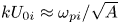 $k U_{0i} \approx \omega _{pi}/\sqrt {A}$, where
 $A = 1 + (1/k^2\lambda _{De}^2)$, and with
 $\omega \ll kU_{0i}$ and
 $\omega \ll \nu _i$, (2.3) has the approximate solution
 \begin{equation} \frac{\omega}{\omega_{pd}} \approx \frac{(1+i)}{\sqrt{2}} \left(\frac{\omega_{pi}} {\nu_i}\right)^{1/2} \frac{1}{A^{3/4}} - \frac{i\nu_d}{2\omega_{pd}}. \end{equation}
2.2. Parameters
In terrestrial experiments, dust grains are often levitated by the electric field in the plasma sheath or presheath. In this region, ions flow toward the sheath with flow speeds much larger than the ion thermal speed. We consider ion flow speeds of a few times the ion thermal speed, which would be expected to lead to a strong ion–dust streaming instability, and thus higher wave amplitudes. In addition, we consider conditions where the frequency of ion and dust collisions with neutrals is a significant fraction of their respective plasma frequencies. We note that this collisional regime may be relevant to dust wave experiments with relatively high pressure (see e.g. Liu et al. Reference Liu, Goree, Flanagan, Sen, Tiwari, Ganguli and Crabtree2018).
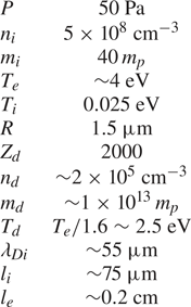
A set of possible nominal dusty plasma parameters, not intended to model any specific experiment, is given in table 1 for an argon plasma containing dust of uniform radius  $R$.
‘Nominal’ parameters.

Here,  $P$ is the argon gas pressure,
 $m_p$ is the proton mass and
 $\lambda _{Di}$ is the ion Debye length. In addition,
 $l_i$ (
 $l_e$) is the ion (electron) mean free path:
 $l_i = (\sigma _{in} n_n)^{-1}$, where
 $n_n$ is the neutral density and the ion–neutral cross-section
 $\sigma _{in} \sim 10^{-14}\ \textrm {cm}^2$;
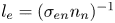 $l_e = (\sigma _{en}n_n)^{-1}$ with
 $\sigma _{en} \sim 5 \times 10^{-16}\ \textrm {cm}^2$. The dust negative charge state
 $Z_d$ was estimated to be reduced by a factor of approximately 3–4 from the collisionless orbit-motion-limited value, owing to the effect of ion–neutral collisions (see e.g. Ratynskaia et al. Reference Ratynskaia, Khrapak, Zobnin, Thoma, Kretschmer, Usachev, Yaroshenko, Quinn, Morfill and Petrov2004; Khrapak et al. Reference Khrapak, Ratynskaia, Zobnin, Usachev, Yaroshenko, Thoma, Kretschmer, Hofner, Morfill and Petrov2005) as well as the effect of electron depletion since
 $Z_dn_d/n_e$ is larger than unity (Havnes, Morfill & Goertz Reference Havnes, Morfill and Goertz1984). With these parameters, the ratio of the ion–neutral collision frequency
 $\nu _i \sim v_i/l_i$ to
 $\omega _{pi}$ is
 $\nu _i/\omega _{pi} \sim 0.5$. The dust–neutral collision frequency is given by
 $\nu _d \sim \delta (4\sqrt {8 {\rm \pi} }/3) R^2 n_n v_n (m_n/m_d)$ where
 $v_n = (T_n/m_n)^{1/2}$, with
 $T_n$ and
 $m_n$ being the temperature and mass of the neutrals, respectively. We take
 $v_n=v_i$ and the factor
 $\delta \sim 1.4$ corresponding to diffuse scattering with full accommodation (Khrapak, Ivlev & Morfill Reference Khrapak, Ivlev and Morfill2004). Then the ratio of
 $\nu _d$ to the dust plasma frequency
 $\omega _{pd} = (4 {\rm \pi} n_d Z_d^2 e^2/m_d)^{1/2}$ is
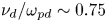 $\nu _d/\omega _{pd} \sim 0.75$. In addition, for these parameters, the ratio of the dust acoustic speed,
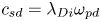 $c_{sd} = \lambda _{Di} \omega _{pd}$ to the dust thermal speed is
 $c_{sd}/v_d \sim 4$.
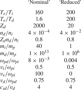
Because we need to use a time step in the simulations that is a small fraction of  $\omega _{pi}^{-1}$, it is time consuming to run a simulation with the possible nominal parameters shown in table 1. Thus we model the linearly unstable spectrum with a ‘reduced’ set of dimensionless parameters, which are given in table 2, along with the dimensionless parameters corresponding to the ‘nominal’ parameters in table 1. In addition, we take the ion flow speed to be
 $U_{0i} = 3 v_i$. Because
 $\nu _e$ (and
 $\omega$) are
 $\ll kv_e$ for the ‘nominal’ parameters, the electrons are kinetic with
 $\zeta _e \ll 1$, so the electron susceptibility is
 $\approx 1/k^2 \lambda _{De}^2$. Thus we can neglect
 $\nu _e$ for the ‘reduced’ parameters. Note that the ratio
 $\omega _{pd}/\omega _{pi} \ll 1$ for both sets of parameters, and the ordering
 $\omega _{pd} \ll \nu _i < \omega _{pi}$ holds for both sets as well.
Dimensionless parameters.

2.3. Linear instability
The frequency and growth rate of the linear ion–dust streaming instability can be obtained by solving (2.2) for  $\omega = \omega _r + i \gamma$, where
 $\gamma > 0$ indicates growth. We assume that the ion flow speed
 $U_{0i}$ is superthermal, as would be expected for ions entering the sheath or presheath where dust may be levitated in terrestrial laboratory experiments. Taking
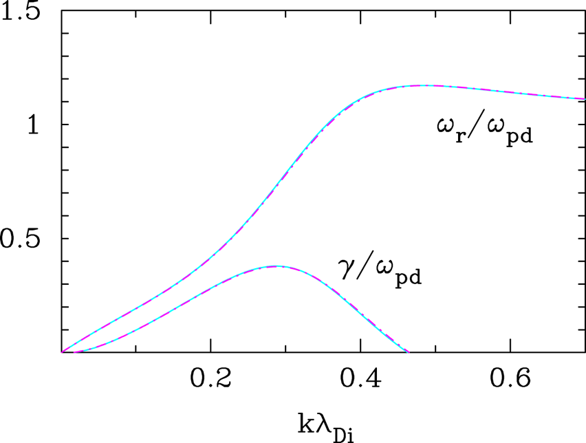
 $U_{0i}/v_i = 3$, figure 1 shows solutions of (2.2) for the two sets of parameters of table 2. As can be seen, both sets of parameters yield ostensibly the same results for the linear instability. Thus we use the set of reduced parameters for the simulations.
Solution of the kinetic dispersion relation (2.2), for parameters in table 2 for normalised real frequency  $\omega _r/\omega _{pd}$ and growth rate
 $\gamma /\omega _{pd}$. The ion drift speed is
 $U_{i0} = 3 v_i$. The cyan solid curves correspond to the nominal parameters, while the magenta dot-dash curves correspond to the reduced parameters.

3. Simulations
3.1. Approach
The simulation runs were performed with a 1-D electrostatic particle-in-cell (PIC) code with periodic boundary conditions (Rosenberg, Quest & Kercher Reference Rosenberg, Quest and Kercher2018). The plasma particle species in the PIC simulation consists of singly charged ions that stream in the  $x$-direction relative to multiply charged heavy dust grains that are stationary in the simulation reference frame. Because we consider the parameter range of figure 1, where
 $kl_e \gg 1$ holds reasonably well for the unstable spectrum, the electrons are treated as Boltzmann distributed and act to provide charge neutrality. The ions and dust are treated as particles, and both particle species collide with background neutrals whose temperature
 $T_n$ remains constant. Collisional effects are modelled using a Langevin scattering operator with a constant collision frequency for each charged species (Gillespie Reference Gillespie1993). The numerical implementation of the scattering operator is well-established and is described in Lemons et al. (Reference Lemons, Lackman, Jones and Winske1995) and Winske & Rosenberg (Reference Winske and Rosenberg1998). There is a background electric field
 ${\boldsymbol {E}}_0 = E_0\,\boldsymbol {x}$, whose magnitude is set such that the corresponding electric force on the ions balances the ion–neutral collision force to maintain a particular ion drift velocity
 ${\boldsymbol {U}}_{i0} = U_{i0}\,\boldsymbol {x}$ during the growth phase of the instability. The magnitude of the electric field is given by the approximate expression
 $E_0 = m_i\nu _i U_{i0}/e$. The only forces on the ion and dust species are an imposed constant electric field (the driver field), a self-consistent electrostatic field generated by the charge separation, and collisional neutral drag. A nonlinear Poisson equation is used to obtain the self-consistent wave potential
 $\phi$. The electron number density takes the form
 $n_e = n_{e0}\exp (e\phi /T_e)$ consistent with the Boltzmann approximation. Together with the ion and dust charge densities, the Poisson equation is then solved by standard iterative means (Hockney & Eastwood Reference Hockney and Eastwood1981). There is a background magnetic field
 ${\boldsymbol {B}}_0 = B_0\,\boldsymbol {x}$, but because it is aligned with both the background electric field and the ion drift, it has no effect on the evolution of the plasma in the
 $x$-direction.
Quantities in the simulation are normalised to ion quantities at the beginning of the simulation. Temperatures and drift speeds are normalised to  $T_{i0}$ and
 $v_{i0}$, which are the initial ion temperature and thermal speed, respectively, and the neutral temperature
 $T_n = T_{i0}$. Length scales are normalised to the ion Debye length
 $\lambda _{Di}$ evaluated at
 $T_{i0}$ and the initial ion density
 $n_{i0}$, while time scales are normalised to the ion plasma frequency
 $\omega _{pi}$ at the beginning of the simulation. The wave electrostatic potential energy
 $e\phi$ is normalised to
 $T_{i0}$ (in energy units) and the wave electric field
 $\tilde {E}$ is normalised to
 $E_r = T_{i0}/e\lambda _{Di}$. In this 1-D simulation, the system length is
 $256 \lambda _{Di}$ and is divided into 256 computational cells. To reduce the numerical noise, the ions and dust are modelled assuming approximately
 $2 \times 10^5$ macroparticles for each particle species.
3.2. Results
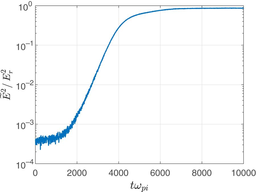
We first present results for a simulation run with the initial conditions corresponding to the ‘reduced’ parameters, which we refer to as case A. The average wave electric field energy (note  $\tilde {E}^2/E_r^2 = \tilde {E}^2/4 {\rm \pi} n_{i0} T_{i0}$) versus time is shown in figure 2. The initial drift speed of the ions is taken to be
 $U_{0i} = 3 v_i$ as in figure 1, while the dust has zero drift. The initial dust temperature is taken to be
 $T_{i0}$. The system is in a growth phase from
 $t\omega _{pi} \sim 2000\text {--}4000$. Estimating
 $\gamma \sim 0.35 \omega _{pd}$ from figure 1, this is approximately three linear growth times. Calculating the logarithmic slope of
 $\tilde {E}^2$ between the times
 $t \omega _{pi} = 2500\text {--}3500$ yields an estimate of growth rate
 $\gamma \sim 0.0014 \omega _{pi} \sim 0.35 \omega _{pd}$ which is in reasonable agreement with the maximum growth rate in figure 1.
Average wave electric field energy versus time for simulation run with ‘reduced’ parameters as initial conditions referred to as case A.

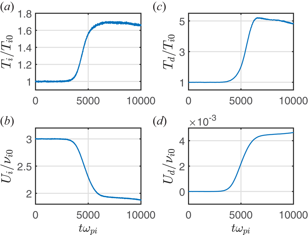
The time histories of the ion and dust temperatures and drift speeds, all averaged over the simulation domain, are shown in figure 3. As can be seen, both the dust and ion temperatures have increased in the nonlinear phase after saturation of the wave energy at  $t \omega _{pi} \gtrsim 5000$, while the dust speed increases and the ion drift speed decreases. With a dust temperature of
 $\sim 4.5 T_{i0}$ and an ion temperature of
 $\sim 1.6 T_{i0}$ at
 $t \omega _{pi} \sim 6000$, the dust acoustic speed is still larger than thermal, with
 $c_{sd} \gtrsim 2.4 v_d$. The dust drift speed
 $U_d \lesssim c_{sd}$ in this nonlinear stage.
Temperatures and drift speeds versus time for case A simulation.  $(a)$ Ion temperature,
 $(b)$ ion drift speed,
 $(c)$ dust temperature,
 $(d)$ dust drift speed.

The increase in dust and ion temperatures appear to be due to wave trapping, although the effect of trapping is reduced owing to collisions which tend to de-trap, which will be discussed later. The condition for trapping is (e.g. Winske Reference Winske2004)
 \begin{equation} Z_j e \phi = \frac{m_j}{2} \left(U_{j0} - \frac{\omega_{\max}}{k_{\max}}\right)^2, \end{equation}
where  $k_{\max }$ is the wavenumber of the dominant mode that traps the particles. For ions, this condition becomes
 $e\phi /T_{i0} \sim m_i U_{0i}^2/2T_{i0} \sim 4.5$. For dust,
 $U_{d0} =0$, and taking
 $k_{\max } \lambda _{Di} \sim v_i/U_{0i} \sim 1/3$ at the resonance condition, with
 $\omega _{\max } \sim \omega _{pd}$ (cf. figure 1), we have that
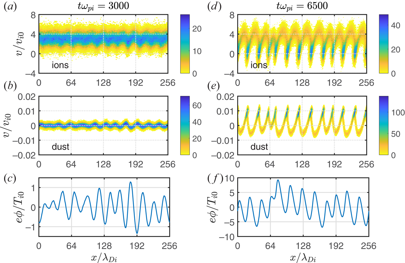
 $e\phi /T_{i0} \sim 4.5 (Z_dn_{d0}/n_{i0}) \sim 3.6$. Figure 4 shows phase space plots and the spatial structure of the wave potential for two times in the simulation:
 $t \omega _{pi} = 3000$ in the linear phase, figure 4(a–c), and
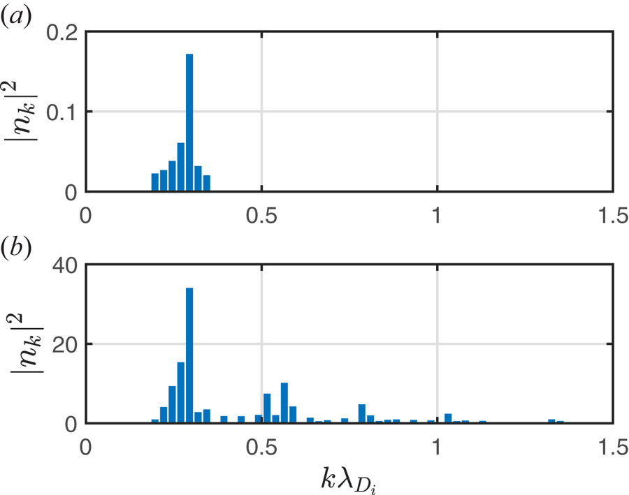
 $t\omega _{pi} = 6500$ in the nonlinear phase, figure 4(d–\,f). The wave potential is large enough to trap both ions and dust in the nonlinear phase, as can be seen from the phase space plots in figure 4(d,e). For this case, from the phase space plots as well as the wave potential plots in figure 4, the dominant wavelength appears to be roughly comparable at both times in the evolution of the system. This can also be seen by analysing the spatial structure of the dust density, i.e. the spatial waveform of the dust density wave. Figure 5 shows the quantity
 $\vert n_k \vert ^2$, which is proportional to the power in the
 $k$ modes of the dust charge density fluctuations, at two times:
 $t \omega _{pi} = 3000$ in the linear phase and
 $t \omega _{pi} = 6500$ in the nonlinear phase. Formally,
 $n_k$ are the Fourier series coefficients of
 $Z_dn_d/n_{i0}$ (note
 $Z_d$ is constant) chosen to obey Parseval's theorem (Oppenheim, Willsky & Nawab Reference Oppenheim, Willsky and Nawab1996). As can be seen by comparing figures 5(a) and 5(b), the dominant wavelengths appear to be similar at both times, with roughly
 $k \lambda _{Di} \sim 0.3$. However, in the nonlinear phase higher harmonics appear as indicated in figure 5(b).
Phase space plots and spatial structure of the wave potential at two times in the case A simulation:  $t \omega _{pi} = 3000$ (a–c) and
 $t \omega _{pi} = 6500$ (d–\,f). Ion phase space plots are shown in panel (a,d), dust phase space plots are shown in panel (b,e) and the wave potential is shown in panel (c,\,f).

Power in the different  $k$-modes of the dust charge density fluctuations at two times: (a)
 $t \omega _{pi} = 3000$, (b)
 $t \omega _{pi} = 6500$.

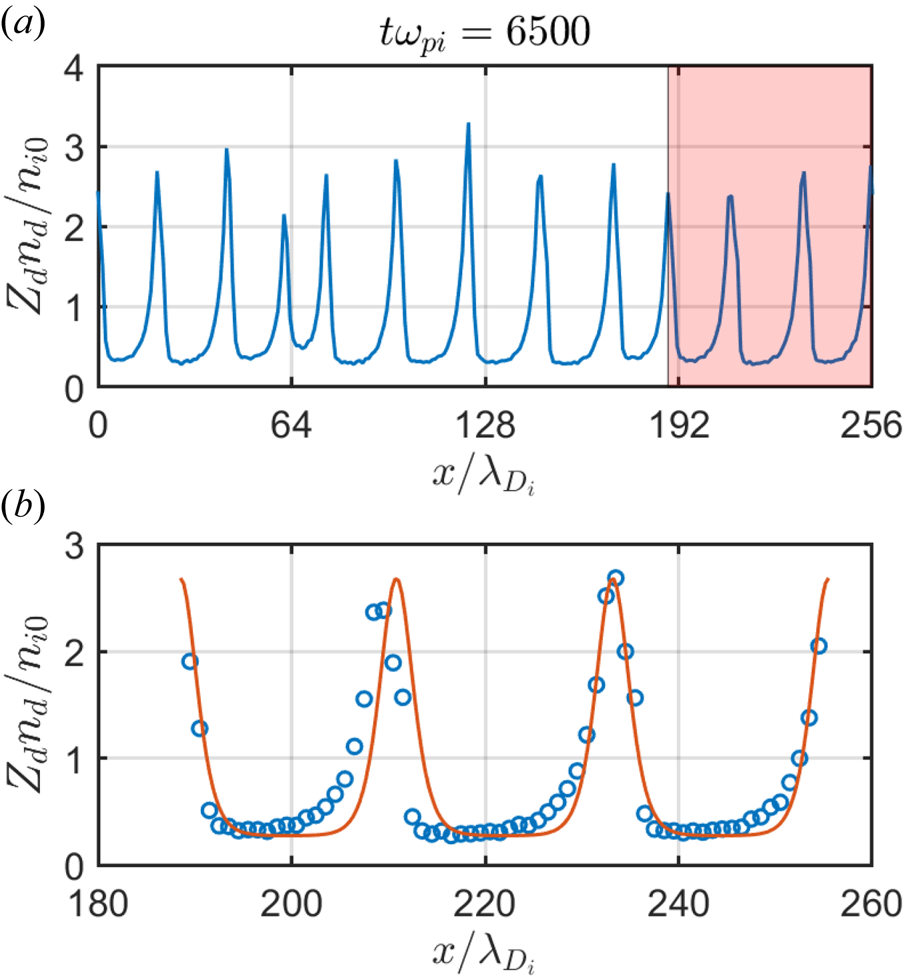
Figure 6(a) shows that the spatial structure of the dust density at  $t \omega _{pi} = 6500$ in the nonlinear phase has a cnoidal-like structure. This type of waveform, with sharper crests and flatter troughs, has a resemblance to nonlinear dust density waves observed in dust wave experiments such as those shown in, for example, Teng et al. (Reference Teng, Chang, Tseng and I2009), Heinrich et al. (Reference Heinrich, Kim, Meyer and Merlino2011) and Merlino et al. (Reference Merlino, Heinrich, Hyun and Meyer2012).
 $(a)$ Spatial structure of the dust density (note
 $Z_d$ is constant) for case A simulation at time
 $t \omega _{pi} = 6500$.
 $(b)$ Comparison of the dust charge density from the simulation (open circles) with a cnoidal function given by (3.2) with
 $p$ = 0.9991 and
 $\lambda = 22.33 \lambda _{Di}$, over the shaded spatial region in panel
 $(a)$.

Motivated by recent experimental observations of cnoidal waveforms of dust density (Liu et al. Reference Liu, Goree, Flanagan, Sen, Tiwari, Ganguli and Crabtree2018), we have attempted to fit the waveform of the dust charge density shown in figure 6(a) to a cnoidal wave solution of the KdV equation. While the latter paper presented cnoidal wave fits of wave data at a specific spatial location, we perform the fit at a specific time, where the cnoidal wave has the form (see Liu et al. Reference Liu, Goree, Flanagan, Sen, Tiwari, Ganguli and Crabtree2018)
 \begin{equation} D(x) = \beta_{\min} + (\beta_{\max} - \beta_{\min})\,cn^2 \left[2 K(p) \left( \frac{x - x_0}{\lambda} \right) ; p \right]. \end{equation}
Here  $D= Z_dn_d/n_{i0}$;
 $\beta _{\min }$,
 $\beta _{\max }$ are the minimum, maximum amplitudes of
 $D$; the function
 $cn$ is a Jacobi elliptic function with elliptic parameter
 $p$;
 $K(p)$ is the complete elliptic integral of the first kind;
 $\lambda$ is the wavelength of the waveform. We selected a portion of the dust density waveform shown in the shaded region in figure 6(a), beginning with a peak, and set
 $x_0$ such that
 $x-x_0 = 0$ in (3.2) at the beginning peak. In addition, we estimate
 $\lambda$ as the average distance between peaks. Using a least squares fit routine, the parameter
 $p$ in (3.2) was optimised. Figure 6(b) shows a comparison of the simulation data (open circles) with the expression (3.2) with
 $p = 0.9991$ and
 $\lambda = 22.33 \lambda _{Di}$ (solid curve). Though there are differences of the data points from the curve, particularly in trough regions, we may surmise the waveform appears to be roughly cnoidal-like.
The results of this simulation suggests the following physical picture. The ion flow excites waves predominantly near the resonance condition that can trap and heat ions and dust when the wave potential becomes large enough. However, collisions can de-trap the particles when the collision rate becomes comparable to the bounce frequency of a particle in the wave (e.g. Nishikawa & Wakatani Reference Nishikawa and Wakatani1990),
 \begin{equation} \nu_{bj} \sim \left(\frac{Z_jek_{\max}\tilde{E}}{m_j}\right)^{1/2}. \end{equation}
In the normalised units of the simulation,
 \begin{equation} \frac{\nu_{bi}}{\omega_{pi}} \sim \left( k_{\max}\lambda_{Di} \frac{\tilde{E}}{E_r} \right)^{1/2} \sim \left( \frac{Z_dn_{d0}}{n_{i0}} \right)^{1/2} \, \frac{\nu_{bd}}{\omega_{pd}}. \end{equation}
Using  $k_{\max }\lambda _{Di} \sim 1/3$ and taking
 $\tilde {E}/E_r \sim 1$ in the nonlinear phase at
 $t \omega _{pi} = 6500$ (cf. figure 2), we have that roughly
 $\nu _{bi}$ is comparable to the ion collision rate
 $\nu _i$, and
 $\nu _{bd}$ is comparable to the dust collision rate
 $\nu _d$. Thus, while the wave tends to trap particles, collisions tend to de-trap, and the increase in the dust temperature remains relatively small so that the dust is essentially ‘cold’ in the nonlinear phase, in that the ratio of the dust acoustic speed to the dust thermal speed is
 $\gtrsim 2.5$. Thus the dust could be treated theoretically using a fluid description. The KdV equation, which is derived from a fluid description of the plasma, has been used to model dust acoustic waves and allows a cnoidal solution for superthermal ion flow speeds (see Liu et al. Reference Liu, Goree, Flanagan, Sen, Tiwari, Ganguli and Crabtree2018). This suggests that a condition for the simulations to show cnoidal-like dust density waveforms may be that the dust remains cold in the nonlinear phase, in addition to a strong instability leading to high amplitude waves.
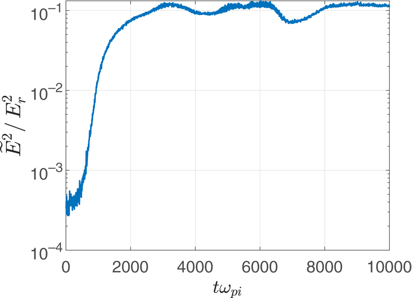
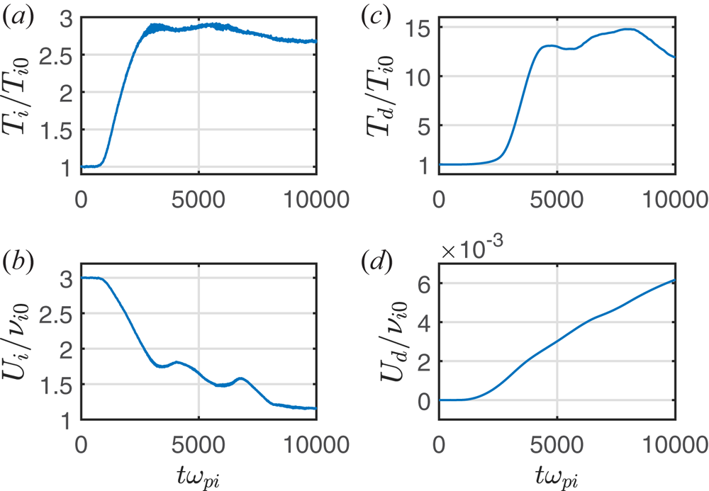
For comparison, we show the results of a simulation with the same initial conditions as in the previous simulation, but in which the ion and dust collision rates have been reduced by a factor of 10, which we refer to as case B. Figure 7 shows the average wave electric field energy density versus time. As expected, the growth phase is shorter for this system, and the maximum wave energy density is smaller than in the high collisionality case.The time histories of the ion and dust temperatures and drift speeds, all averaged over the simulation domain, are shown in figure 8. Comparing with figure 3, it can be seen that the ion and dust temperature increase is much larger. At  $t \omega _{pi} \sim 5000$ in the nonlinear phase, where
 $T_d$ has increased by a factor of
 $\sim 15$, the ratio
 $c_{sd}/v_d \sim 1.8$, while the ion flow speed has decreased to near
 $1.5v_i$, so that the ion–dust streaming instability becomes a weaker semikinetic instability in this nonlinear phase. We estimate the trapping frequency in the nonlinear phase at
 $t \omega _{pi} \sim 5000$ where
 $\tilde {E}/E_r \sim 0.3$ from figure 7. This yields a ratio of
 $\nu _{bi}/\nu _i \sim 6$ for the ions, and
 $\nu _{bd}/\nu _d \sim 5$ for the dust. Thus de-trapping by collisions is weak, consistent with the larger increase in ion and dust temperatures.
Average wave electric field energy versus time for simulation run with ‘reduced’ parameters as initial conditions but with collision rates reduced by 1/10, referred to as case B.

Temperatures and drift speeds versus time for case B simulation.  $(a)$ Ion temperature,
 $(b)$ ion drift speed,
 $(c)$ dust temperature,
 $(d)$ dust drift speed.

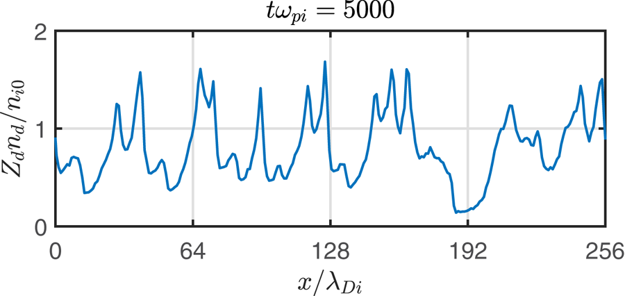
Finally, figure 9 shows the waveform of the dust charge density in the nonlinear phase at  $t \omega _{pi} = 5000$, which does not exhibit the cnoidal-like structures shown in figure 6 for the high collisionality case.
Spatial structure of the dust density (note  $Z_d$ is constant) for case B simulation at time
 $t \omega _{pi} = 5000$.

4. Summary and discussion
We have presented 1-D PIC simulations of the nonlinear development of an ion–dust streaming instability, driven by ions with superthermal flow speed, in a highly collisional plasma. For the parameter set we considered, the collision rate of ions and negatively charged dust with neutrals is a significant fraction of their respective plasma frequencies. This collisional regime may be representative of microgravity or laboratory dust wave experiments with high neutral gas pressure. The simulations show that in the nonlinear regime, the waveforms of the dust density assume coherent structures with broad troughs and sharp peaks, which appear roughly to be cnoidal-like. Further, several harmonics of the dominant mode excited in the linear phase arise in the wave spectrum in the nonlinear phase. The dust temperature does not increase very much in the nonlinear phase, likely because the dust–neutral collision rate is larger than the trapping frequency of dust.
Because the dust remains cold, in the sense that the dust acoustic speed is sufficiently larger than the dust thermal speed, this suggests that the nonlinear dust waves may be described using a fluid description. It was shown in Liu et al. (Reference Liu, Goree, Flanagan, Sen, Tiwari, Ganguli and Crabtree2018) that a KdV equation for the nonlinear dust acoustic wave can be obtained using a cold ion ‘ballistic’ response for the streaming ions and that a solution of this KdV equation is a chain of solitons, or a cnoidal wave solution. The cnoidal function was shown by Liu et al. (Reference Liu, Goree, Flanagan, Sen, Tiwari, Ganguli and Crabtree2018) to fit well their experimental waveforms of dust number density over a wide range of amplitudes. As the dust density amplitudes in figure 6 are fairly large, it would be interesting in future work to see how the theory in Liu et al. (Reference Liu, Goree, Flanagan, Sen, Tiwari, Ganguli and Crabtree2018) may apply to this simulation result.
We compared the simulation results with another simulation run with the same parameters but with the ion and dust collision rates reduced by a factor of 10, primarily to show the difference in the waveforms of dust density in the nonlinear phase. The dust density was not observed to have coherent cnoidal-like structures, and the dust temperature increased significantly.
This study only considered one set of parameters, and future work should scope out the range of parameters under which dust density waveforms with flattened troughs and sharp crests appear in the nonlinear phase, in order to make contact with experimental observations of such structures. A limitation of the present study is that it is a 1-D simulation. Depending on plasma and dust parameters, the growth rate of dust waves due to the ion–dust streaming instability can maximise in directions different from the direction of ion flow when the ion flow is superthermal (see e.g. Rosenberg Reference Rosenberg1996; Piel et al. Reference Piel, Klindworth, Arp, Melzer and Wolter2006). Thus future work should also consider the two-dimensional case. In addition, the present analysis applies to dusty plasmas in the weakly coupled phase, and future work should consider the effect of strong dust coupling.
Acknowledgements
This work was supported by NSF grants PHY-1613102 and PHY-1740203.
Editor Edward Thomas thanks the referees for their advice in evaluating this article.
Declaration of interests
The authors report no conflict of interest.