INTRODUCTION
Meltwaters from the Laurentide Ice Sheet during the last deglaciation became dammed behind terminal and recessional moraines, creating a series of glacial lakes in southern New England (Stone and Borns, Reference Stone and Borns1986; Dyke and Prest, Reference Dyke and Prest1987; Uchupi et al., Reference Uchupi, Driscoll, Ballard and Bolmer2001; Fig. 1). These proglacial lakes persisted for thousands of years while accumulating vast amounts of water and sediment (Uchupi et al., Reference Uchupi, Driscoll, Ballard and Bolmer2001). Moraine-dammed glacial lakes can drain either gradually or in a rapid, catastrophic manner (Veillette, Reference Veillette1994) that abruptly releases massive amounts of water (Richardson and Reynolds, Reference Richardson and Reynolds2000). Such floods cause substantial erosion, incising previous deposits and creating distinct morphology (Clayton and Knox, Reference Clayton and Knox2008). The drainage of some large glacial lakes may have played an important role in climate cooling by freshening the North Atlantic and causing a slowdown of thermohaline circulation (Alley et al., Reference Alley, Mayewski, Sowers, Stuiver, Taylor and Clark1997; Barber et al., Reference Barber, Dyke, Hillaire-Marcel, Jennings, Andrews, Kerwin and Bilodeau1999; Teller et al., Reference Teller, Leverington and Mann2002; Donnelly et al., Reference Donnelly, Driscoll, Uchupi, Keigwin, Schwab, Thieler and Swift2005).
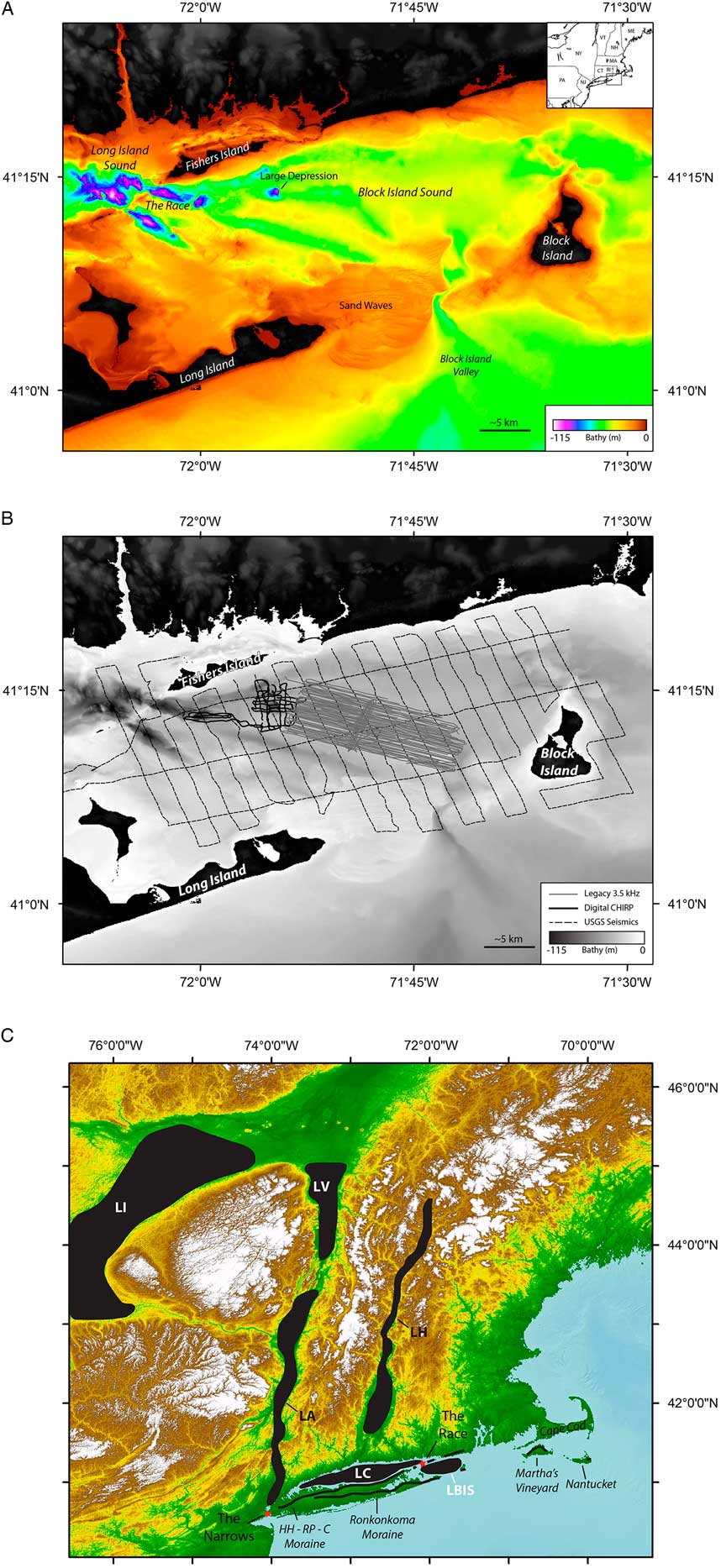
(color online) (A) Regional bathymetric map showing major features in study area. Bathymetry is from the coastal relief model (National Geophysical Data Center [NGDC], 1999), the National Oceanic and Atmospheric Administration (NOAA) tsunami inundation Montauk zone (Eakins et al., Reference Eakins, Taylor, Carignan, Warnken, Sazonova and Schoolcraft2009), and NOAA multibeam interpreted by the USGS (Poppe et al., Reference Poppe, DiGiacomo-Cohen, Doran, Smith, Stewart and Forfinski2007, Reference Poppe, McMullen, Danforth, Blankenship, Clos, Glomb, Lewit, Nadeau, Wood and Parker2014b). An inset shows the study area in New England. (B) Trackline map for seismic surveys. Legacy CHIRP profiles collected in 1995 on the R/V Henlopen are shown in gray, digital CHIRP collected in 1999 on the SSV Westward are in solid black (lines are less than straight, because data were collected by a sailing vessel), and USGS uniboom seismics are shown with black dashed lines (Needell and Lewis, Reference Needell and Lewis1984; Poppe et al., Reference Poppe, Paskevich, Lewis and DiGiacomo-Cohen2002). (C) Map showing major glacial lakes in the region. Moraines are shown by thick black lines. Red stars denote constriction points referred to in the paper. HH–RP–C, Harbor Hill–Roanoke Point–Charlestown moraine; LA, Lake Albany; LBIS, Lake Block Island Sound; LC, Lake Connecticut; LH, Lake Hitchcock; LI, Lake Iroquois; LV, Lake Vermont.

Glacial lake Block Island Sound (Lake BIS) was a proglacial lake that formed behind the terminal moraine of the Laurentide Ice Sheet in present-day Block Island Sound (BIS), offshore from Rhode Island (Fig. 1). In the early 1980s, a seismic-reflection survey was performed in BIS to define the sound’s Quaternary geologic history (Needell and Lewis, Reference Needell and Lewis1984; Poppe et al., Reference Poppe, Paskevich, Lewis and DiGiacomo-Cohen2002; Fig. 1B). This survey revealed six major depressions in the seafloor between 60 and 100 m below modern sea level (Fig. 1A). Some of the depressions are more elongated, with a southeast orientation, while others are more circular in map view. The depressions are located around the spillway at the Race (Fig. 1A and C), which separated glacial Lake BIS from glacial Lake Connecticut. Glacial Lake Connecticut formerly occupied modern-day Long Island Sound (Fig. 1A and C). The origin of these depressions was proposed to be modern tidal currents scouring near constriction zones (Lewis and Stone, Reference Lewis and Stone1991). In this interpretation, the glacial lakes gradually drained together without deep erosional downcutting or scouring (Lewis and Stone, Reference Lewis and Stone1991). Other work (Uchupi et al., Reference Uchupi, Driscoll, Ballard and Bolmer2001) suggested a catastrophic draining of the lakes, with Lake BIS draining first, then Lake Connecticut draining ~500 years later through BIS. In the catastrophic scenario, the fast-draining waters of Lake Connecticut would have carved out the depressions as they flowed across the subaerially exposed BIS.
Here we present high-resolution subbottom and bathymetry data to evaluate these alternative models and provide new insights into margin evolution along glaciated regions. Results from this study reveal the styles of erosional morphology caused by glacial lake outburst floods across a low-gradient ice margin. It is important to note that erosion and downcutting along glaciated margins may be out of phase with eustatic sea-level fluctuations, as glacial lake outburst floods and incision often occur during a eustatic sea-level transgression. This study also finds that there was not significant reworking of the morphology in the BIS region, providing an important constraint on the rate of sea-level transgression and its impacts at these water depths. These insights may explain otherwise anomalous morphologic features observed along other low-gradient glaciated margins.
REGIONAL SETTING
Deglaciation of southern New England
BIS is located just northeast of Long Island Sound in southern New England (Fig. 1). During the most recent glacial period (Marine Oxygen Isotope Stage 2 [MIS 2]), the southern lobe of the Laurentide Ice Sheet extended across southern New England, mantling the inner continental shelf. The ice sheet reached its maximum extent between ~23 and 24 ka before retreating, leaving behind a series of moraines (Stone and Borns, Reference Stone and Borns1986; Dyke and Prest, Reference Dyke and Prest1987; Uchupi et al., Reference Uchupi, Driscoll, Ballard and Bolmer2001; Fig. 1C). Long Island, Cape Cod, and Block Island are subaerial remnants of the terminal moraines (Oldale and O’Hara, Reference Oldale and O’Hara1980; Sirkin, Reference Sirkin1982; Fig. 1C), composed mainly of glaciofluvial sands and gravels and layers of diamicton (Colgan et al., Reference Colgan, Mickelson and Cutler2003). As the ice retreated, other glacial deposits formed, including drumlin fields, (Colgan et al., Reference Colgan, Mickelson and Cutler2003), kames and eskers (Poppe et al., Reference Poppe, DiGiacomo-Cohen, Smith, Stewart and Forfinski2006), kettle hole lakes (Damman and French, Reference Damman and French1987), and recessional moraines (Sirkin, Reference Sirkin1982, Reference Sirkin1991; Uchupi et al., Reference Uchupi, Driscoll, Ballard and Bolmer2001). Meltwaters sourced from the Laurentide Ice Sheet were dammed by both recessional and terminal moraines, creating an extensive glacial lake system (Fig. 1C). From about 17 to 15 ka, most of the lakes drained across the then-exposed shelf, carving out valleys and depressions that still exhibit a bathymetric expression today. Hudson Shelf valley and Block Island valley are such examples (Uchupi et al, Reference Uchupi, Driscoll, Ballard and Bolmer2001; Donnelly et al., Reference Donnelly, Driscoll, Uchupi, Keigwin, Schwab, Thieler and Swift2005; Thieler et al., Reference Thieler, Butman, Schwab, Allison, Driscoll, Donnelly and Uchupi2007; Fig. 2).
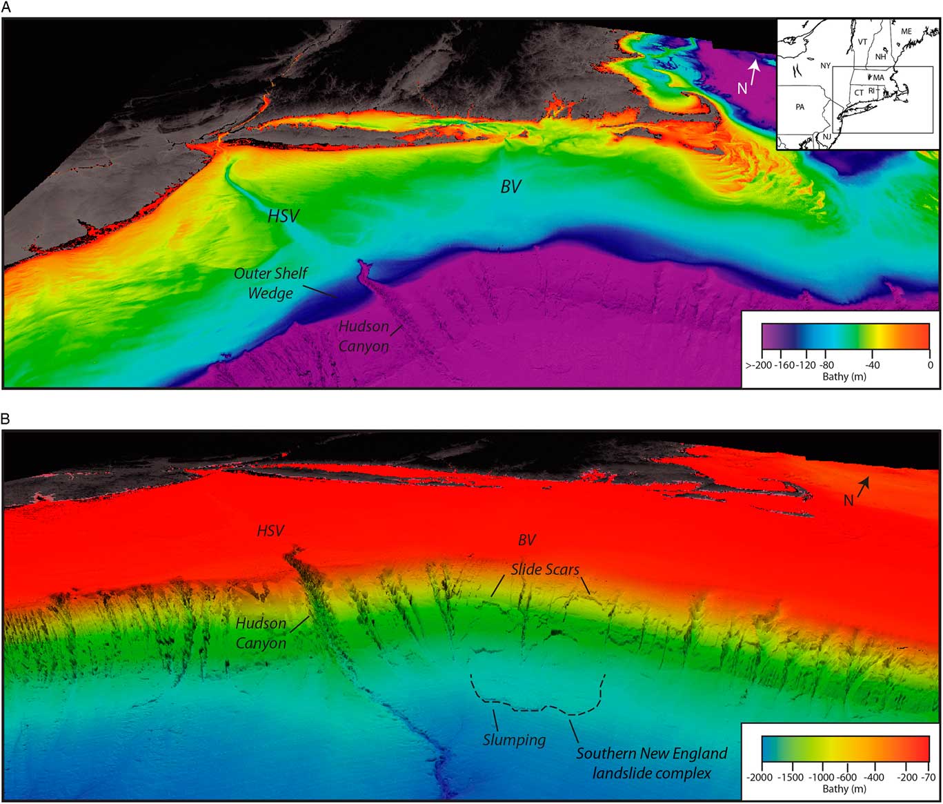
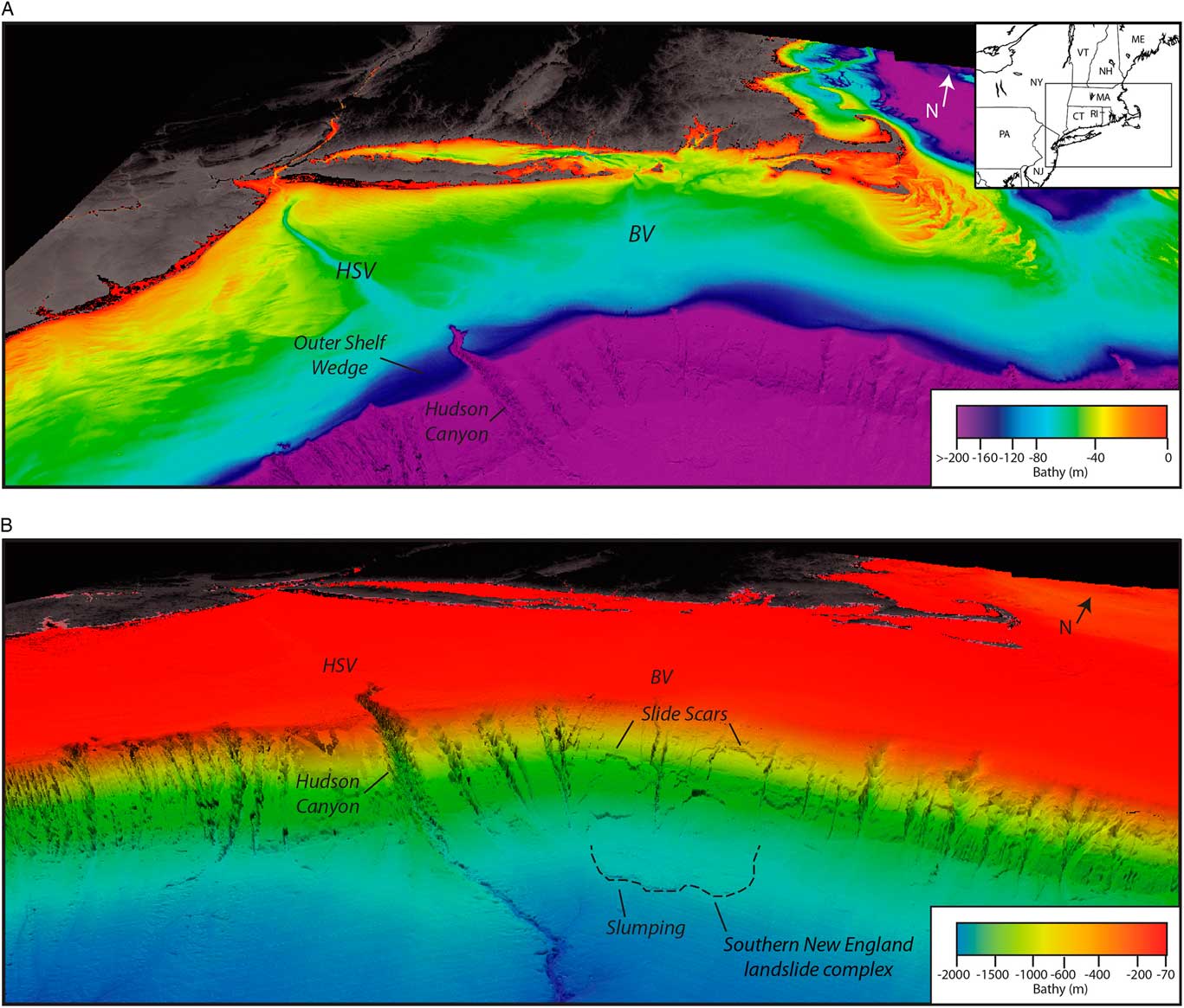
(color online) Regional perspective bathymetry images of the study region (VE 15×). (A) Perspective image of shelf bathymetry highlighting the Hudson Shelf valley, Block Island valley, and the outer-shelf wedge at the distal end of Hudson Shelf valley. Inset shows the displayed region. (B) Slope morphology for the region is shown. Hudson Shelf valley leads into a large canyon (Hudson Canyon) at the shelf edge that continues down slope into a channel on the rise. South of Block Island valley on the slope are slide scars and slump complexes (outlined by a dashed black line). Bathymetry data are from the coastal relief model (NGDC, 1999), data collected by the University of New Hampshire for the US related to the UN Law of the Sea (Gardner et al., Reference Gardner, Mayer and Armstrong2006), and from the USGS (Andrews et al., Reference Andrews, Chaytor, ten Brink, Brothers, Gardner, Lobecker and Calder2016). BV, Block Island valley; HSV, Hudson Shelf valley.
Geology of BIS
BIS has a complicated history, which in turn has created complex morphology and stratigraphy. The bedrock underlying the sound consists of pre-Mesozoic igneous and metamorphic rocks that dip toward the south (McMaster et al., Reference McMaster, Lachance and Garrison1968; Bertoni et al., Reference Bertoni, Dowling and Frankel1977; Lewis and DiGiacomo-Cohen, Reference Lewis and DiGiacomo-Cohen2000). The crystalline basement on Block Island is composed of gneisses, schists, and granitic intrusions, similar to the mainland (Woodworth et al., Reference Woodworth, Wigglesworth, Berry, Bryan, Hollick and Stephenson1934). Throughout the sound, the basement rock has been dissected by an extensive Tertiary drainage system generally trending toward the south-southeast (McMaster et al., Reference McMaster, Lachance and Garrison1968; McMaster and Ashraf, Reference McMaster and Ashraf1973). The bedrock in BIS is, in some places, overlain by Cretaceous coastal plain sediments (Needell and Lewis, Reference Needell and Lewis1984). This unit is composed of unconsolidated to semiconsolidated gravels, sands, silts, and clays (Lewis and DiGiacomo-Cohen, Reference Lewis and DiGiacomo-Cohen2000) but is often found interspersed with glacial deposits on land from glacial reworking. In seismic profiles from Needell and Lewis (Reference Needell and Lewis1984), the difference between the coastal plain strata and the basement rock is often difficult to discern, with the main difference being that the coastal plain strata locally exhibit faint internal reflectors. As such, they were combined for a depth-to-stratigraphic-surface map. These basal layers are commonly overlain by two glacial drift sheets, one attributed to a late-MIS 2 ice advance and the other to a previous ice advance (Sirkin, Reference Sirkin1982; Needell and Lewis, Reference Needell and Lewis1984; Lewis and Stone, Reference Lewis and Stone1991).
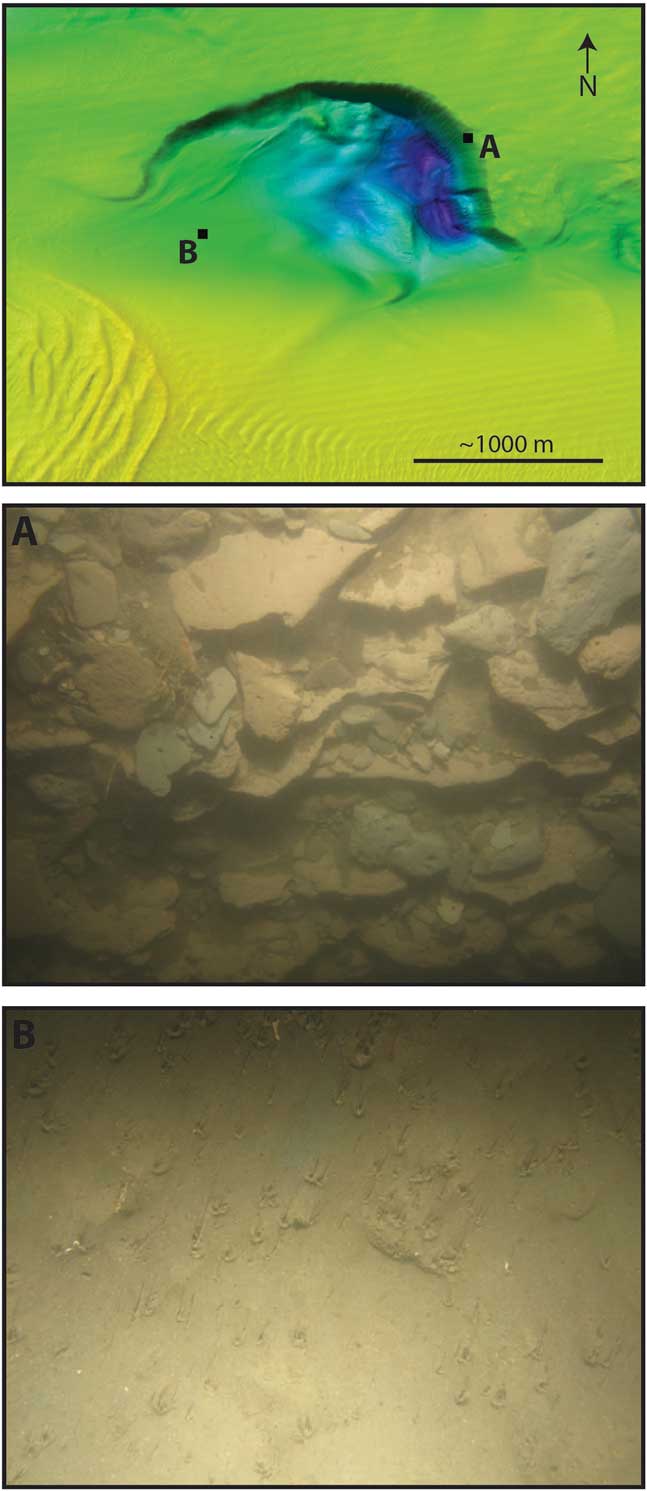
The southern terminal moraine for the Laurentide Ice Sheet is the Ronkonkoma–Block Island–Nantucket moraine, deposited between ~23 and 24 ka (Balco et al., Reference Balco, Stone, Porter and Caffee2002; Fig. 1C), which forms part of Long Island, Block Island, and Martha’s Vineyard. The Harbor Hill–Roanoke Point–Charlestown recessional moraine was deposited between ~18 and 19 ka and extends from northern Long Island, across Fishers Island, onto the mainland (Balco et al., Reference Balco, Stone, Porter and Caffee2002; Fig. 1C). The moraines are mostly composed of boulders, layered sands and gravels, sediment flow materials, and till (Stone et al., Reference Stone, DiGiacomo-Cohen, Lewis and Goldsmith1998). The Harbor Hill–Roanoke Point–Charlestown recessional moraine created a barrier between Long Island Sound and BIS, separating glacial Lake Connecticut and glacial Lake BIS (Fig. 1C). The water surface of Lake BIS is estimated to have been ~20 m below present sea level, given a low in the glacial moraine topography at this level (Boothroyd et al., Reference Boothroyd, Freedman, Brenner and Stone1998). During the existence of glacial Lake BIS, glaciolacustrine varve sediments were deposited (Needell and Lewis, Reference Needell and Lewis1984). Sediment cores and photos from these deposits confirm that they are composed of layered reddish-brown and gray silts and clays (Bertoni et al., Reference Bertoni, Dowling and Frankel1977; McMullen et al., Reference McMullen, Poppe, Danforth, Blackwood, Clos and Parker2014; Fig. 3). After the lake drained, BIS was exposed subaerially and eroded by fluvial processes (Uchupi et al., Reference Uchupi, Driscoll, Ballard and Bolmer2001).
The Laurentide Ice Sheet caused BIS to be isostatically depressed. Recent estimates by Oakley and Boothroyd (Reference Oakley and Boothroyd2012) suggest that the depression was no more than 35 m, less than prior estimates (Andrews, Reference Andrews1973; Lewis and Stone, Reference Lewis and Stone1991; Stone et al., Reference Stone, Shafer, London, DiGiacomo-Cohen, Lewis and Thompson2005). The regional linear uplift profile is between 0.7 and 1.0 m/km (Koteff and Larson, Reference Koteff and Larsen1989; Stanford and Harper, Reference Stanford and Harper1991; Koteff et al., Reference Koteff, Robinson, Goldsmith and Thompson1993; Rayburn, Reference Rayburn2004). Marine incursion of the region likely happened after isostatic rebound started (Oakley and Boothroyd, Reference Oakley and Boothroyd2012). If rebound was slow enough, marine waters could have entered BIS within 1000 years of the lake draining (Lewis and Stone, Reference Lewis and Stone1991). As sea level rose, estuarine and marsh sediments were deposited, followed by beach and bar deposits (Lewis and DiGiacomo-Cohen, Reference Lewis and DiGiacomo-Cohen2000). Reworking continues today by strong tidal currents (Lewis and DiGiacomo-Cohen, Reference Lewis and DiGiacomo-Cohen2000) that reach up to 4 knots (Poppe et al., Reference Poppe, DiGiacomo-Cohen, Doran, Smith, Stewart and Forfinski2007), as well as by storm waves. The current seafloor sediment ranges from boulders and gravels to silty sands depending on the energy environment (Poppe et al., Reference Poppe, Danforth, McMullen, Blakenship, Glomb, Wright and Smith2014a), with the finer sediments deposited in the deeper, outer parts of the sound.
DATA ACQUISITION AND PROCESSING
In 1999, high-resolution CHIRP seismic data were acquired in BIS. The survey was conducted using an EdgeTech X-Star CHIRP subbottom seismic-reflection sonar with submeter vertical resolution. The CHIRP system was towed a few meters below the surface by Sea Education Association’s SSV Westward. The tracklines are more curvilinear than straight, because the SSV Westward is a sailing vessel. The profiles were acquired using a 1–6 kHz swept-frequency acoustic source, which allowed for seafloor penetration up to 50 m. All data were recorded in SEG-Y format with real-time GPS navigation recorded with each shot for location accuracy. The data were processed using SIOSEIS (Henkart, Reference Henkart2003) and then imported into the Kingdom software package for interpretation. A nominal value of 1500 m/s was applied to convert two-way travel time to depth; both are shown on seismic profiles. Legacy paper 3.5 kHz seismic records from the early 1990s, acquired on the R/V Henlopen, were converted to digital SEG-Y using the Matlab code image2segy.m (Farran, Reference Farran2008; http://gma.icm.csic.es/node/67 [accessed February 20, 2015]) and also imported into Kingdom Suite. A detailed description of the conversion procedure is provided in the Supplementary Material. Additionally, an early 1980s U.S. Geological Survey (USGS) uniboom seismic-reflection survey was examined for comparison to the newer data sets (Needell and Lewis, Reference Needell and Lewis1984; Poppe et al., Reference Poppe, Paskevich, Lewis and DiGiacomo-Cohen2002). Several high-resolution, multibeam data sets were used to examine the seafloor morphology in BIS and the outer shelf and slope offshore of the study area (Gardner et al., Reference Gardner, Mayer and Armstrong2006; Poppe et al., Reference Poppe, DiGiacomo-Cohen, Doran, Smith, Stewart and Forfinski2007, Reference Poppe, Danforth, McMullen, Blakenship, Glomb, Wright and Smith2014a, Reference Poppe, McMullen, Danforth, Blankenship, Clos, Glomb, Lewit, Nadeau, Wood and Parker2014b; Andrews et al., Reference Andrews, Chaytor, ten Brink, Brothers, Gardner, Lobecker and Calder2016).
MAPPING RESULTS
Acoustic units and stratigraphy
Four clearly defined acoustic units are observed throughout the surveyed area, described below from oldest to youngest. The interpretation of each of these units is based on their acoustic character, stratigraphic geometry, history of the area, and seismic interpretation by previous studies (e.g., Needell and Lewis, Reference Needell and Lewis1984; Lewis and Stone, Reference Lewis and Stone1991; Poppe et al., Reference Poppe, DiGiacomo-Cohen, Smith, Stewart and Forfinski2006).
The deepest unit observed throughout the study region is defined as acoustic basement. Core data and outcrops show that acoustic basement consists of an undifferentiated mixture of bedrock, coastal plain strata, and glacial moraine deposits (Bertoni et al., Reference Bertoni, Dowling and Frankel1977; Needell and Lewis, Reference Needell and Lewis1984; Fig. 4). The acoustic basement has a high-amplitude acoustic character with few internal reflectors. The character of the reflector at the top of the acoustic basement varies laterally, ranging from a crisp, sharp reflector to a more blotchy acoustic boundary (Figs. 4–6, Supplementary Fig. 1). This observed variation in acoustic character does not correlate with the over 40 m of relief on the acoustic basement. The acoustic basement often exhibits a rounded, mound-like morphology and crops out at the seafloor in some regions (Figs. 4 and 5).
(color online) Photographs of sedimentary deposits in the large depression (McMullen et al., Reference McMullen, Poppe, Danforth, Blackwood, Clos and Parker2014). The top image shows photo location. Scales were not published for the photographs. (A) Photograph 298_36d from the steep wall of the depression where the glaciolacustrine varve deposits crop out on the seafloor. The layers are composed of reddish-brown and gray silty clay, along with rip-up clasts. Evidence of bioturbation in the clasts is present, along with hydrozoans. (B) Photograph 298_12a from the gradually sloping southwest entrance to the large depression. Based on a grain-size sample (McMullen et al., Reference McMullen, Poppe, Danforth, Blackwood, Clos and Parker2014), the seafloor here is composed of fine sand and is heavily bioturbated. Scours have formed around objects, delineating the dominant flow direction.

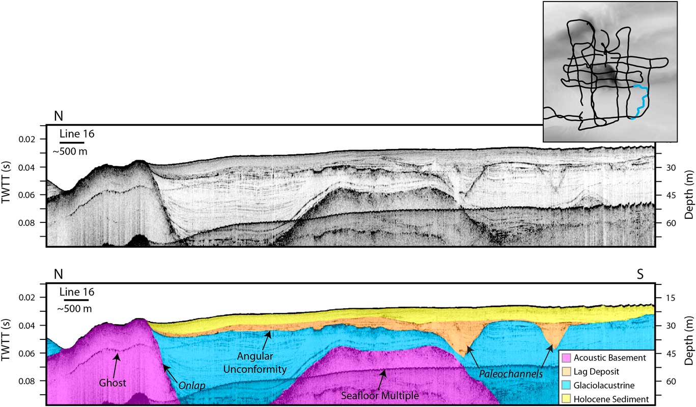
CHIRP line 16 uninterpreted (top) and interpreted (bottom). The trackline is highlighted in blue on the inset. Inset trackline locations also are shown for Figures 5–7. There are major channels cut into the glaciolacustrine sediment that have been infilled. The Holocene sediment and lag deposit onlap onto an exposure of acoustic basement in the northern part of the profile. (For interpretation of the references to color in this figure legend, the reader is referred to the web version of this article.)

The next unit is a glaciolacustrine deposit (Fig. 3) that exhibits a well-laminated acoustic character (Figs. 4–6, Supplementary Fig. 1). The laminations are predominantly parallel and mimic the shape of the underlying acoustic basement. Such sediment draping is indicative of low-energy lacustrine environments in which sediment is largely deposited from suspension. Nevertheless, some layers do exhibit minor thickness variations, with their thickness increasing toward the topographic lows (Figs. 4 and 6). Where the glaciolacustrine sediments crop out at the seafloor, their surface is smoother (northern region: Fig. 6); however, where buried, their boundary has more relief and exhibits a hummocky, scalloped morphology (southern region: Fig. 6, Supplementary Fig. 2) with notches (Supplementary Fig. 1). The thickness of the glaciolacustrine sediments varies markedly from a thin veneer to thicknesses greater than 50 m (Fig. 5, Supplementary Fig. 3). The large depression cuts into the glaciolacustrine deposits, exposing the layered silts and clays (Fig. 3).
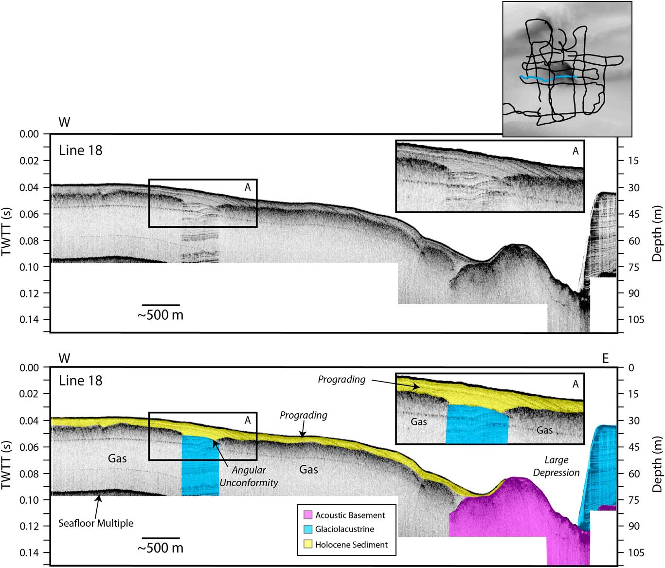
(color online) CHIRP line 18. Seismic imaging and penetration is limited by gas in the sediments. Where the glaciolacustrine unit is visible, the boundary between this layer and the Holocene sediment above can be observed. The Holocene sediment is prograding downslope (inset A shows an enlargement), where it onlaps onto a high in the acoustic basement. This high is sufficient to block the sediment from infilling the large depression to the east.

The modern transgressive surface separates the underlying glaciolacustrine unit from the overlying sediments (Figs. 4–7, Supplementary Figs. 1–4). Another erosional surface is observed at the top of the glaciolacustrine unit and has a V-shaped morphology (Figs. 4 and 7). These V-shaped paleochannels range from a few meters to more than a kilometer in width (Fig. 4, Supplementary Figs. 2 and 3). The smaller paleochannels observed in CHIRP line 32 (Supplementary Fig. 3) have a high-amplitude reflector that delineates the base of the channels, which may be the result of gas charging along the boundary or a coarser lag deposit.
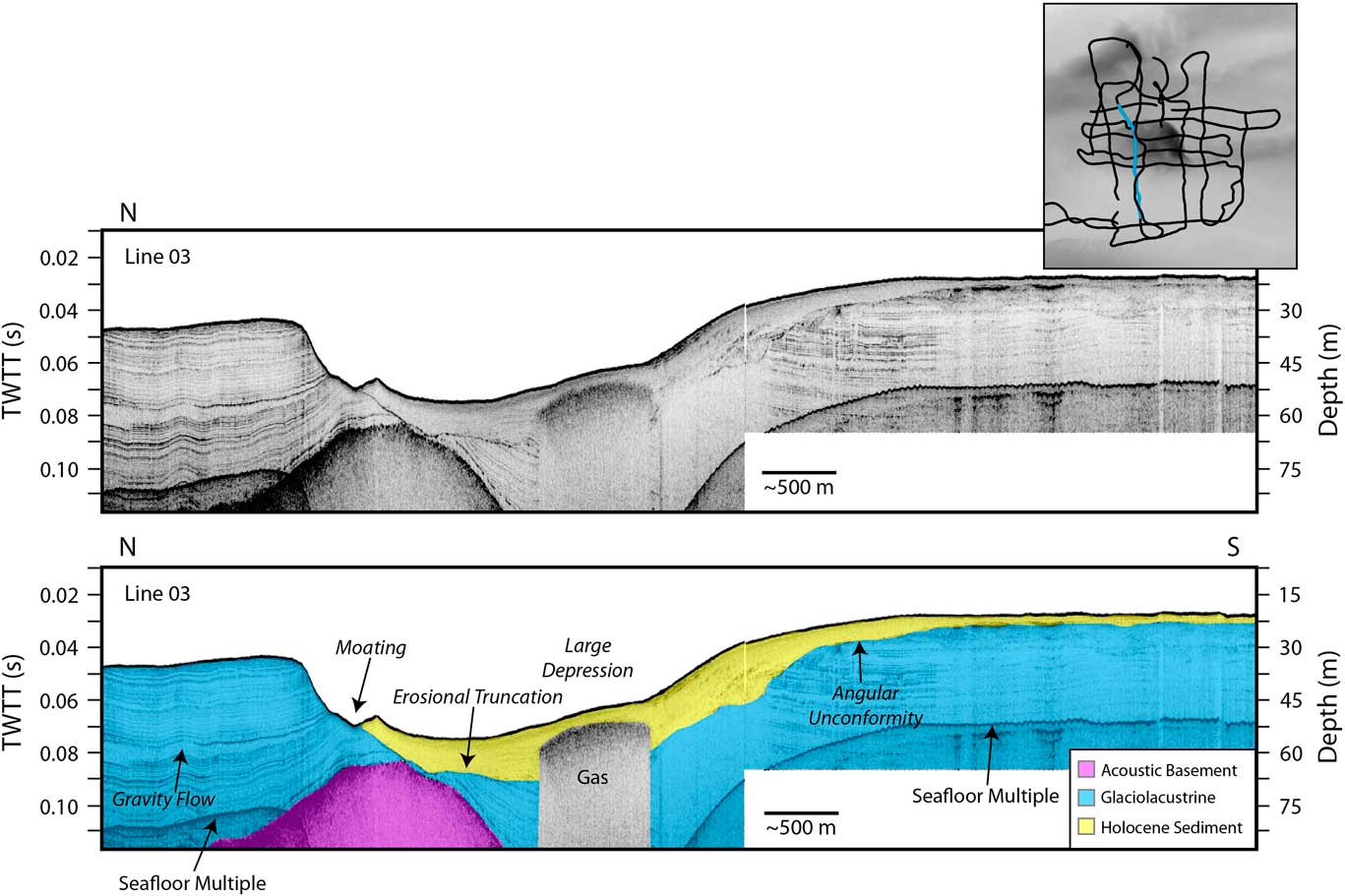
(color online) CHIRP line 03. A gas wipeout in the data is labeled. There is a marked erosional unconformity in the glaciolacustrine layer that is covered by Holocene sediment. The Holocene sediments have also been shaped by currents.

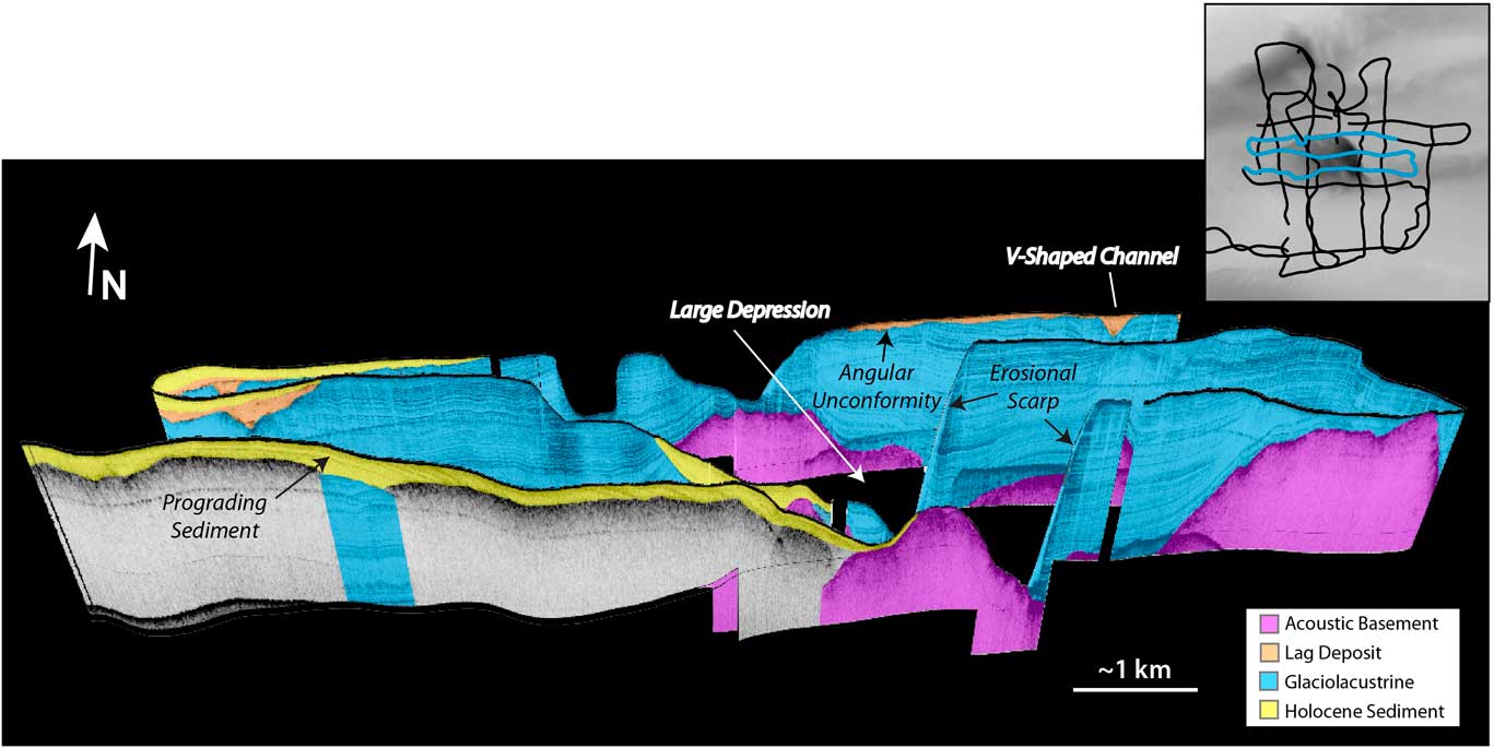
Perspective view looking north at the large depression. Profiles shown are highlighted in blue on the trackline map. Holocene sediment is observed prograding down into the depression but is blocked by a high in the acoustic basement. (For interpretation of the references to color in this figure legend, the reader is referred to the web version of this article.)

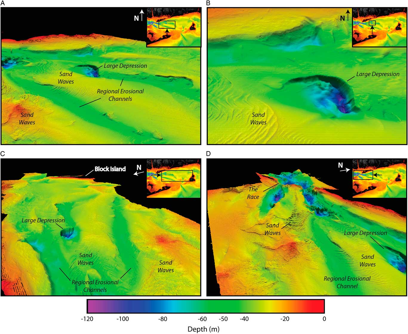
(color online) Perspective scenes of high-resolution bathymetry in BIS collected by NOAA and interpreted by the USGS (VE 15×) (Poppe et al., Reference Poppe, DiGiacomo-Cohen, Doran, Smith, Stewart and Forfinski2007, Reference Poppe, McMullen, Danforth, Blankenship, Clos, Glomb, Lewit, Nadeau, Wood and Parker2014b). Each image has an inset of BIS, with a box and arrow showing the image extent and view direction. (A) Looking north toward the large depression. Regional erosional channels and sand waves are observed around the large depression. (B) Close-up of the large depression. The gradually sloping western side and the steep eastern wall of the depression are imaged. (C) Looking east toward Block Island showing the regional erosional channels trending toward the entrance to BIS. (D) Looking west toward Long Island Sound at the Race. This image highlights the deep elongate depressions at the connection between the two sounds. The transition from the Race to the regional erosional channels is imaged.

The third unit infills paleochannels and overlies the glaciolacustrine sediments (Figs. 4 and 7, Supplementary Figs. 2 and 3). This unit has abundant internal reflectors, with some reflectors more organized and linear, while others are more chaotic in nature, with high acoustic reflectivity (Fig. 4). Thickness of the unit is quite variable (Supplementary Fig. 2) and is largely formed on the interchannel highs (Figs. 7 and 8). Where it fills in channels, the unit reaches thicknesses greater than 15 m but thins away from these localized depocenters (Fig. 4). Because the unit fills in lows and has high acoustic character, it is defined as a lag deposit composed of coarser, reworked sediment (e.g., fluvial and estuarine). This sediment unit was deposited after the transgression, which provides an age maximum for deposition. Estimates for marine incursion in this region are as old as ~15 ka (Lewis and Stone, Reference Lewis and Stone1991) and as young as ~12.5 ka (Donnelly et al., Reference Donnelly, Driscoll, Uchupi, Keigwin, Schwab, Thieler and Swift2005).
The upper unit is defined as posttransgressive sediment of Holocene age (Needell and Lewis, Reference Needell and Lewis1984). It is referred to as “Holocene sediment” throughout the rest of the article. The unit overlies the lag deposit, so it is younger in age, most likely being mid- to late Holocene. The Holocene unit has some internal acoustic reflectors, but large areas are acoustically transparent (Figs. 4, 6, and 7). Prograding reflectors are observed to be migrating downslope, originating in shallow water and then pinching out onto a high in the acoustic basement (Figs. 5 and 7). Sculpting of the sediment layer is also observed along the steep erosional unconformity in the glaciolacustrine sediments (Fig. 5, Supplementary Fig. 1). The Holocene sediment thickness ranges from less than 1 m to approximately 20 m (Supplementary Fig. 1). In the shallow regions, symmetric and asymmetric bedforms composed of Holocene sediment are observed (Figs. 4 and 8, Supplementary Fig. 1).
Physiography
The large, circular depression in the seafloor is referred to as the “large depression” and is ~100 m below modern sea level (Figs. 1, 3, and 8). The eastern slope is quite steep (~18°) while the western side is much more gradual (Figs. 5 and 8B). The glaciolacustrine sediments are exposed at the seafloor along the steep eastern side of the depression (Figs. 5, 6 and 7). There is an absence of Holocene sediments within the deepest part of the depression (Fig. 7), but they are observed on the southwestern side of the depression, prograding to the east (Figs. 5 and 7, Supplementary Fig. 1).
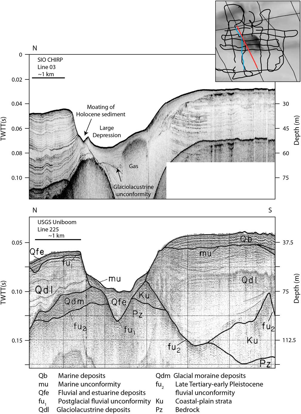
Comparison of digital CHIRP line 03 (top) and USGS uniboom line 225 (bottom; Needell and Lewis, Reference Needell and Lewis1984; Poppe et al., Reference Poppe, Paskevich, Lewis and DiGiacomo-Cohen2002). CHIRP line 03 has a different vertical exaggeration than in Figure 6 for comparison to the uniboom line. The location of the CHIRP line is highlighted in blue on the inset, and the uniboom line is highlighted in red. Interpretations for uniboom line 225 are from Needell and Lewis (Reference Needell and Lewis1984). The CHIRP profile is higher resolution, while the uniboom line has deeper penetration as a result of acquisition frequencies. (For interpretation of the references to color in this figure legend, the reader is referred to the web version of this article.)

Two large erosional channels (between 40 and 60 m depth; Fig. 8) connect the Race to the outlet at Block Island valley. The channels are separated by a shoal (~30 m depth), which is mantled by sediment waves (Fig. 8A and D). The large circular depression is located near the mouth of the northern erosional channel. Elongate erosional depressions are imaged near the Race between Long Island Sound and BIS (between ~80 and 120 m depth; Fig. 8A and D). The sediment waves observed in the region are largely confined to the shoals (~30 m depth) and exhibit a variety of morphologies from linear to arcuate.
DISCUSSION
Glacial lake drainage and development of inner-shelf morphology
The complex morphology of BIS appears to have developed in multiple stages (Needell and Lewis, Reference Needell and Lewis1984), driven primarily by glacial lake drainage. Two main conceptual models have been proposed to explain the observed morphology and subbottom reflectors in BIS (Bertoni et al., Reference Bertoni, Dowling and Frankel1977; Needell and Lewis, Reference Needell and Lewis1984; Lewis and Stone, Reference Lewis and Stone1991; Uchupi et al., Reference Uchupi, Driscoll, Ballard and Bolmer2001; Poppe et al., Reference Poppe, McMullen, Danforth, Blankenship, Clos, Glomb, Lewit, Nadeau, Wood and Parker2014b; McMullen et al., Reference McMullen, Poppe, Danforth, Blackwood, Winner and Parker2015). Both conceptual models ascribe the regional erosional channels imaged in the bathymetry to glacial lake drainage, with subsequent overprinting by fluvial and storm processes (Needell and Lewis, Reference Needell and Lewis1984; Lewis and Stone, Reference Lewis and Stone1991; Uchupi et al., Reference Uchupi, Driscoll, Ballard and Bolmer2001; McMullen et al., Reference McMullen, Poppe, Danforth, Blackwood, Clos and Parker2014; McMullen et al., Reference McMullen, Poppe, Danforth, Blackwood, Winner and Parker2015; Poppe et al., Reference Poppe, Danforth, McMullen, Blakenship, Glomb, Wright and Smith2014a; Fig. 8, Supplementary Figs. 2 and 3). The manner in which the glacial lakes drained and how the large depressions formed differs between the two models.
The first conceptual model suggests that Lake Connecticut and Lake BIS drained gradually, at the same time. In this model, erosion of the spillway between the lakes (at the Race) was controlled by the rate of draining of Lake BIS (Lewis and Stone, Reference Lewis and Stone1991; Stone et al., Reference Stone, DiGiacomo-Cohen, Lewis and Goldsmith1998). The authors estimated that the lakes were completely drained by 15.5 ka based on estimates of delta building and coarse material in the upper-lake varve deposits as Lake Connecticut drained (Lewis and Stone, Reference Lewis and Stone1991). The erosion and formation of the depressions by the Race are attributed to modern tidal-current erosion caused by constriction from the Harbor Hill recessional moraine (Bertoni et al., Reference Bertoni, Dowling and Frankel1977; Needell and Lewis, Reference Needell and Lewis1984; Lewis and Stone, Reference Lewis and Stone1991; Figs. 1 and 8).
In the other conceptual model, Uchupi et al. (Reference Uchupi, Driscoll, Ballard and Bolmer2001) proposed a near-instantaneous draining of glacial Lake BIS by approximately 16 ka, followed by the catastrophic draining of glacial Lake Connecticut about 500 years later (~15.5 ka). The draining of these lakes would be in the form of glacial lake outburst floods. The timing of the Lake BIS draining is based on sediments from the outer-shelf wedge of the Hudson Shelf valley (Fig. 2) that were interpreted to be deposited ~16 ka, possibly sourced from the draining of Lake BIS and transported by ocean currents (Uchupi et al., Reference Uchupi, Driscoll, Ballard and Bolmer2001). The timing of glacial Lake Connecticut drainage is based on the estimate of Lewis and Stone (Reference Lewis and Stone1991). In this model, formation of the large depression and the depressions near the Race are the result of erosion and scouring during rapid lake draining (Figs. 1 and 8). The new CHIRP and bathymetry data support the rapid-draining model.
Interpretation of the CHIRP data indicate that the large depression formed before the transgression and deposition of Holocene sediments (Fig. 6), which is consistent with a catastrophic draining of the glacial lakes and not with a modern tidal-scour origin. The boundary between the Holocene sediment and the underlying glaciolacustrine sediments within the large depression is observed in the CHIRP data (Figs. 6 and 9). The uniboom seismic data did not image the glaciolacustrine sediments beneath this boundary (Fig. 9); consequently, Needell and Lewis (Reference Needell and Lewis1984) interpreted this boundary as a postglacial fluvial unconformity, indicating the depression was formed by river drainage during subaerial exposure of BIS. The scale of the depression is much larger than other postglacial fluvial features (i.e., Supplementary Figs. 2 and 3), and the morphology is not typical of a river channel (Figs. 1A and 8). Based on stratal geometry observed in this region, our preferred interpretation is that the glaciolacustrine sediments were truncated during a glacial lake outburst flood, with additional erosion from fluvial and storm runoff during subaerial exposure.
Development of outer-shelf and slope morphology
When glacial Lake BIS and Lake Connecticut existed, the continental shelf adjacent to BIS would have been sediment-starved, as the lakes would be efficient sediment traps. This is consistent with the delta deposits observed along their northern margins (Lewis and Stone, Reference Lewis and Stone1991). When the lakes drained, they would have transported large volumes of sediment offshore. High-resolution bathymetric data along the continental shelf and slope exhibit morphologic features that are consistent with the proposed outburst flood model (Gardner et al., Reference Gardner, Mayer and Armstrong2006; Andrews et al., Reference Andrews, Chaytor, ten Brink, Brothers, Gardner, Lobecker and Calder2016; Fig. 2). Block Island valley extends from the entrance of BIS across the shelf (Figs. 1 and 2), and slide scars and slump deposits are observed on the adjacent continental slope (e.g., the southern New England landslide complex; Fig. 2B). When the Lake BIS outburst flood occurred, the flows would have eroded Block Island valley and deposited sediment toward the shelf edge and slope. This process would have been repeated when Lake Connecticut drained. Rapid deposition on the continental slope could also explain the observed slope failures (Fig. 2; Driscoll et al., Reference Driscoll, Weissel and Goff2000). Similar morphology is observed to the southwest at Hudson Shelf valley, where glacial lake outburst floods from the Lake Albany–Vermont–Iroquois system have also been proposed (Uchupi et al., Reference Uchupi, Driscoll, Ballard and Bolmer2001; Donnelly et al., Reference Donnelly, Driscoll, Uchupi, Keigwin, Schwab, Thieler and Swift2005; Thieler et al., Reference Thieler, Butman, Schwab, Allison, Driscoll, Donnelly and Uchupi2007; Figs. 1C and 2).
Preservation of shelf morphology
Why the complex morphology in BIS has not been eroded and obscured by the recent transgression remains poorly understood (Figs. 1 and 8). During a sea-level transgression, wave-base energy erodes bathymetric highs and infills the lows, diminishing relief (Klotsko et al., Reference Klotsko, Driscoll, Kent and Brothers2015). However, as mentioned earlier, the large depressions and regional erosional valleys in BIS were not reworked and infilled. Block Island valley and Hudson Shelf valley also were not infilled, unlike other previously incised valleys along the Atlantic margin (Thieler et al., Reference Thieler, Butman, Schwab, Allison, Driscoll, Donnelly and Uchupi2007; Fig. 2). Bertoni et al. (Reference Bertoni, Dowling and Frankel1977) suggested that the large depression, referred to as the “big hole” in their paper, is a drowned kettle hole. Many kettle lakes that formed during the deglaciation are observed onshore at Block Island and throughout southern New England, as are drowned kettle holes offshore between western Cape Cod and Martha’s Vineyard (Sirkin and Veeger, Reference Sirkin and Veeger1998; Poppe et al., Reference Poppe, McMullen, Foster, Blackwood, Williams, Ackerman, Barnum and Brennan2008; Fig. 1C). Offshore kettle holes might explain the continued existence of the circular depressions, but not the larger incised valleys. A potential explanation for the preservation of these features is that they are geologically young and the transgression was too rapid in these water depths to significantly rework sediment. As the region was isostatically depressed, the marine incursion could have occurred as early as 15 ka (Lewis and Stone, Reference Lewis and Stone1991), but definitely by ~12.5 ka (Donnelly et al., Reference Donnelly, Driscoll, Uchupi, Keigwin, Schwab, Thieler and Swift2005). The rapid transgression would have drowned the features not long after they were formed, preserving them. Erosion and maintenance of the depressions in BIS (Fig. 8D) result from present-day swift tidal currents nearly 4 knots in speed (Poppe et al., Reference Poppe, DiGiacomo-Cohen, Doran, Smith, Stewart and Forfinski2007), as evidenced by sculpted sediment (Fig. 6) and differential erosion and deposition throughout the sound (Figs. 7 and 8).
Global implications of glacial lake outburst floods
Glacial moraine-dammed lakes are found worldwide, typically in mountainous areas where glaciers have retreated. They commonly drain as outburst floods (Richardson and Reynolds, Reference Richardson and Reynolds2000) from overflowing water that eroded the moraine. The lakes can discharge at rates of 30,000 m3/s and empty within hours (Richardson and Reynolds, Reference Richardson and Reynolds2000). Sediment from the lakes and eroded moraine dams is transported in debris flows and can deposit as fans (Clague and Evans, Reference Clague and Evans2000). Much of the debris from documented glacial lake outburst floods in British Columbia was deposited within a few hundred meters of the breached moraines (Clague and Evans, Reference Clague and Evans2000), but discharges from outburst floods in the Himalayas have traveled more than 200 km (Richardson and Reynolds, Reference Richardson and Reynolds2000). The initial outburst can transport large boulders, up to 200 tons, hundreds of meters from the lake (Evans and Clague, Reference Evans and Clague1994). Outburst floods from larger lakes can erode valleys downstream before depositing their sediment load (Clague and Evans, Reference Clague and Evans2000).
Studying past moraine-dammed glacial lake outburst floods allows us to better assess the stability of modern glacial lake systems and understand the potential extent of flood damage. Modern outburst floods have caused major destruction of property, land, and infrastructure and significant loss of life (Yongjian and Jingshi, Reference Yongjian and Jingshi1992), with more than 30,000 people killed by these types of floods in the last 100 years (Richardson and Reynolds, Reference Richardson and Reynolds2000). In areas like Nepal, Bhutan, and Tibet, there is a constant threat of more glacial lake outburst floods, which would devastate many rural communities (Richardson and Reynolds, Reference Richardson and Reynolds2000; Kattelmann, Reference Kattelmann2003). The potential hazard is only increasing as glaciers retreat in response to climatic warming (Richardson and Reynolds, Reference Richardson and Reynolds2000).
This study revealed the far-reaching effects of glacial lake outburst floods on a low-gradient shelf. Waters from Lake Connecticut and Lake BIS traveled more than 150 km, incising the shelf and depositing sediment on the outer shelf and adjacent continental slope. Rapid deposition on continental margins by glacial lake outburst floods could also trigger large submarine-slope failures, as observed on the southern New England landslide complex (Fig. 2B). Submarine landslides can trigger tsunamis and bury offshore infrastructure (Lee et al., Reference Lee, Schwab and Booth1993); information from past slope failures along glaciated margins will help us to understand potential failures associated with glacial lake outburst floods in the future.
Finally, the data from the BIS region provide insights into the deglacial morphology that is observed on other glaciated margins. One important new result is that erosion and downcutting along glaciated margins may be out of phase with eustatic sea-level fluctuations, as glacial lake outburst floods and incision often occur during the eustatic sea-level transgression. Downcutting and fluvial incision along continental margins generally occurs during relative sea-level falls (Christie-Blick and Driscoll, Reference Christie-Blick and Driscoll1995). Morphology developed as a result of glaciation and outburst floods is substantial and often is not significantly reworked or obscured during the transgression, which is typically the case along other continental margins (Klotsko et al., Reference Klotsko, Driscoll, Kent and Brothers2015).
CONCLUSIONS
Analysis of new high-resolution CHIRP seismic and bathymetry data, as well as scanned legacy 3.5 kHz seismic profiles, has provided important constraints on the development of the complex morphology in BIS. These new data have allowed us to refine the model proposed by Lewis and Stone (Reference Lewis and Stone1991) based on seismic profiles interpreted by Needell and Lewis (Reference Needell and Lewis1984). The new CHIRP data image an unconformity separating Holocene sediment from underlying glaciolacustrine sediments in the large depression (Fig. 6), suggesting that the depression was eroded before the transgression. Based on the morphostratigraphy in and around BIS, as well as other studies of glacial lakes, our preferred model is that the depressions and Block Island valley were formed by glacial lake outburst floods. The continuing existence of this morphology may be the result of a rapid transgression across these water depths. The large depression and other morphology in BIS have likely not been infilled during the Holocene due to lack of sediment in the vicinity and swift tidal currents.
Our interpretations of the new data suggest that margin incision associated with glacial lake outburst floods is out of phase with eustatic sea-level rise. The effects of such floods are far-reaching, even on low-gradient margins. The preservation potential for morphology created by glacial lake outburst floods is high, as it is often not reworked by wave-base erosion associated with the eustatic transgression.
ACKNOWLEDGMENTS
We would like to thank the Captain Sean Bercaw and the crew of the SSV Westward for sailing a great survey in BIS and the crew of the R/V Cape Henlopen for their assistance collecting the 3.5 kHz profiles, side-scan data, and VanVeen cores. We thank Colby Nicholsen for his assistance with digitizing the paper seismic records. This research was funded by the Office of Naval Research, with a special thanks to Joseph Kravitz. Educational support for S. Klotsko was provided by a National Science Foundation Graduate Research Fellowship (DGE-1144086).
SUPPLEMENTARY MATERIALS
To view supplementary material for this article, please visit https://doi.org/10.1017/qua.2018.32