1. Introduction
Pollution in various forms exists across the globe, especially in developing nations. Understanding the causes of pollution is a serious research question in economics dating back to the heated debates about the limits to growth in the early 1970s (Meadows et al., Reference Meadows, Meadows, Randers and Behrens1972), as well as being the topic of urgent policy debates today (Auffhammer and Kellogg, Reference Auffhammer and Kellogg2011; Schlenker and Walker, Reference Schlenker and Walker2016). Traditionally, economists have focused on factors such as economic growth (Halkos and Tzeremes, Reference Halkos and Tzeremes2013; Greenstone and Hanna, Reference Greenstone and Hanna2014), or institutions and policies (Cole and Fredriksson, Reference Cole and Fredriksson2009; Acemoglu et al., Reference Acemoglu, Aghion, Bursztyn and Hemous2012; Gibson, Reference Gibson2019) as determinants of pollution. Particular attention is paid to the context of rapidly developing nations such as China (Cai et al., Reference Cai, Lu, Wu and Yu2016; Xu and Li, Reference Xu and Li2023), India (Balietti et al., Reference Balietti, Datta and Veljanoska2022) and Mexico (Arceo et al., Reference Arceo, Hanna and Oliva2016). The determinants, including economic growth, institutions and policies, could be the outcomes of growth preference when officials have to make a trade-off between economy and environment. Yet less is known about how growth preference impacts the environment. This question is fundamental because many theories and empirical evidence in economics support the idea that a set of preferences drives individual decision-making (Falk et al., Reference Falk, Becker, Dohmen, Enke, Huffman and Sunde2018). This includes preferences about risk (Mendogo and Bocquého, Reference Mendogo and Bocquého2024), the timing of rewards (Nursimulu and Bossaerts, Reference Nursimulu and Bossaerts2014) and so on. The officials’ preference for growth indicates their prioritization of economic expansion over other considerations, such as environmental sustainability or social welfare. Given the importance of preferences in economists’ conceptual framework, understanding how growth preference impacts the environment is crucial for fully recognizing the determinants of pollution and gaining insights into institutional arrangements for sustainable development.
Growth preference represents one dimension of fundamental factors affecting officials’ decision-making in environmental protection (Hao et al., Reference Hao, Chen, Liao and Wei2020). Local officials have substantial influence over the local activities by controlling key economic resources, such as land and credit, and designing local policies such as taxation and government spending as well as environmental regulation. Because of their direct influence on the local activities, these officials are able to make a trade-off between economy and environment according to their growth preference. Historically, the economics literature has primarily focused on the causes of growth preference, especially due to economic performance-based promotion scheme (Maskin et al., Reference Maskin, Qian and Xu2000; Li and Zhou, Reference Li and Zhou2005). In terms of the consequence of growth preference, literature has mainly focused on gross domestic product (GDP) growth (Li et al., Reference Li, Liu, Weng and Zhou2019), and rent seeking and corruption (Chen and Kung, Reference Chen and Kung2019), but considerably less on environmental consequences. However, there is evidence showing pollution for promotion (Jia, Reference Jia2024) and fulfilling minimum environmental targets while pursuing the largest possible economic growth (Cao et al., Reference Cao, Weng, Xu and Zhou2021). In this paper, we analyse the environmental consequences of growth preference.
Chinese local officials have traditionally pursued local economic development with tremendous preference for enhancing regional economic growth. This is motivated by the career concerns of local officials. Since the initiation of China's opening-up and reform policy in 1978, the central government has shifted the evaluation criteria for local officials from political performance to economic development, emphasizing economic growth (Song et al., Reference Song, Storesletten and Zilibotti2011; Wu and Cao, Reference Wu and Cao2021; Jia, Reference Jia2024). The economy has become a top priority for the Chinese government, with economic performance serving as a key indicator for officials’ promotions (Liu and Kong, Reference Liu and Kong2021). Consequently, local officials are incentivized to drive rapid economic growth in their jurisdictions in pursuit of political promotion or favourable assessments (He et al., Reference He, Wang and Zhang2020). This paper examines the causal effects of growth preference on ambient pollutant concentrations. As in the pioneering work by Li and Zhou (Reference Li and Zhou2005), we use GDP growth as the measure of economic performance; therefore, changes in GDP growth ranking are a source of variation in growth preference.
The intuition of such variation is straightforward: in China's economic performance-based scheme, local officials link their promotion prospects to local economic growth, especially their performance relative to their peers; therefore, officials in cities experiencing a decline in GDP growth ranking have more incentives to take measures to promote the local economy, even at the cost of more pollutant emissions.
Two main empirical challenges are the small variation in ranking changes and identification. The small variation makes it difficult to precisely estimate the effect because it reduces the statistical power, making it challenging to distinguish the true effect from random noise. The variation in GDP growth ranking changes among Chinese cities is small due to the centralized and coordinated economic policies that lead to similar growth strategies across regions. This coordination, along with intense competition among provinces to meet central government targets, minimizes differences in economic performance. Uniform measurement and reporting practices also contribute to the homogeneity in reported GDP growth, further limiting variation in rankings. To solve this challenge, we leverage the GDP shuffling caused by COVID-19. COVID-19 caused GDP shuffling among China's cities by introducing unprecedented and uneven economic disruptions across regions, significantly increasing the variation in GDP growth rankings. Differences in local infection rates, lockdown measures and industrial compositions led to distinct variations in growth rates, breaking previously coordinated patterns. This increased variation helps address the challenge of small variations, allowing for more precise estimation of the effects of GDP growth changes.
The second challenge, which is general for empirical studies, is to find exogenous variation in growth ranking changes. Local officials are defined as more growth preferred when the city they are working in experienced decline in growth ranking, but the change in growth ranking is not necessarily exogenous. Endogenous factors, such as regional economic policies, industrial composition and natural resource endowments, can simultaneously influence both growth ranking and environmental outcomes. For example, a decline in a city's growth ranking might be due to a regional economic downturn affecting multiple cities in the area. This regional downturn could also affect local environmental outcomes due to transboundary air pollution (Jia and Ku, Reference Jia and Ku2019). Without exogenous variation, it becomes difficult to disentangle the causal relationship between ranking changes and environmental consequences.
To find exogenous variation in ranking changes, we use the number of COVID infected cases of each city during 2020–2022 as the instrumental variable (IV) of growth ranking changes in 2023. It is justified because the COVID-19 pandemic is exogenous to local economic conditions in the context of this study. Cities with higher numbers of COVID infected cases may experience disruptions in economic activity, leading to changes in their growth rankings independent of other local factors. By focusing on COVID infected cases during the pandemic period (i.e., 2020–2022), the instrument is temporally prior to the outcome variable (i.e., 2023), further strengthening its validity. By leveraging this exogenous variation, the IV approach helps isolate the causal effect of growth ranking changes on environmental consequences, addressing the challenge of endogeneity in empirical studies.
Our study makes contributions to several areas of the literature. First, it applies the concept of political preference driving decision-making to government operations. With behaviours being driven by preferences (Falk et al., Reference Falk, Becker, Dohmen, Enke, Huffman and Sunde2018), political preference has been widely explored in theoretical models of government agency behaviour (Dixit, Reference Dixit2009). Yet empirical investigation is challenging due to the difficulty in identifying exogenous variation in political preference. This paper addresses this challenge by leveraging variations in growth preferences arising from growth ranking shocks caused by the COVID-19 pandemic. Although the strong motivation of local officials arising from GDP growth tournament competition may be specific to China, the general implications of how political preferences affect outcomes are broadly applicable.
Second, this study analyses the association between economic ranking changes and pollution levels through the lens of political preference to understand the behaviour of local officials in China. In China, improving the economic growth ranking of their jurisdiction is crucial for the political promotion of local officials. Cities that faced more severe disruptions from the pandemic during 2020–2022 experienced significant drops in their economic rankings. Since economic ranking is a critical performance metric for local officials, those in cities with larger declines during the pandemic had stronger incentives to prioritize economic recovery post-pandemic, often at the expense of environmental regulations. We hypothesize that these cities would show increased pollution levels due to the officials’ focus on boosting economic growth to regain their rankings. Our empirical strategy leverages the uneven impact of COVID-19 on Chinese cities to explore the relationship between economic ranking changes and pollution, driven by the growth preferences of local officials. This approach allows us to identify the causal link between the growth preferences induced by economic ranking changes during pandemic and the variations in pollution levels observed post-pandemic.
Third, our paper contributes to the literature on the political economy of the environment. Emerging research in the context of China highlights the significant role of career concerns in various outcomes. For example, Fu and Viard (Reference Fu, Viard and Leung2022) discuss mayors’ perspectives on addressing air pollution, and Jia (Reference Jia2024) attributes high levels of environmental pollution in China partly to promotion incentives. Additionally, Kong et al. (Reference Kong, Ma and Qin2022) and Xue and Zhang (Reference Xue and Zhang2024) explore how politicians’ career concerns influence local firms’ pollution behaviours, and Cao et al. (Reference Cao, Weng, Xu and Zhou2021) examine the strategic responses of local Chinese officials to the minimum air quality control targets. This study specifically focuses on the fundamental element of career concerns: growth preference. We provide insights into the mechanisms through which growth preference impacts air pollution, thereby adding to the understanding of environmental outcomes in the context of political economy.
The rest of this paper is organized as follows. Section 2 provides an overview of the GDP shuffling among China's cities caused by COVID-19. Section 3 describes the methodology and data utilized in this study. We present the empirical results in Section 4, and Section 5 further discusses cautious behaviours of local officials in balancing economic growth and environmental quality. Finally, Section 6 concludes the study.
2. Background on GDP shuffling caused by COVID-19
Amidst the COVID-19 pandemic during 2020–2022, the Chinese central government implemented comprehensive epidemic containment policies from early 2020 to mitigate virus transmission and protect public health. Stringent measures, including lockdowns and restrictions on movement, were enforced in regions with severe outbreaks to limit the spread of the virus (Kaplan et al., Reference Kaplan, Lefler and Zilberman2022). While these measures were somewhat effective in reducing COVID-19 cases, they also had significant repercussions on economic activities. Janiak et al. (Reference Janiak, Machado and Turén2021) note that the restrictions led to disruptions in the supply chain, reduced production capacity and slowed economic growth. Particularly vulnerable were low-skilled labourers and small enterprises who faced factory closures, layoffs and wage reductions, exacerbating unemployment rates and economic instability. Additionally, lockdown measures prompted individuals to curtail their spending, resulting in decreased revenue for industries such as retail, catering and tourism (Hodbod et al., Reference Hodbod, Hommes, Huber and Salle2021). Consequently, the epidemic prevention and control measures have had profound impacts on economic activities across various regions (Wan and Tian, Reference Wan and Tian2022).
The COVID-19 pandemic created a unique research opportunity, manifesting in GDP shuffling due to widespread economic disruptions. Local growth rankings in China experienced rapid changes during this period, as depicted in the kernel density plot in Figure 1. A notable dispersion in growth rankings change was observed from 2022 to 2019,Footnote 1 contrasting with the period from 2018 to 2016 which was characterized by relative stability. This indicates substantial shuffling in growth rankings across cities during the pandemic. Consequently, cities heavily impacted by COVID-19 were increasingly motivated to revitalize their local economies following the ending of pandemic lockdown in early 2023. This implies a stronger preference towards economic growth when faced with the trade-off between the economy and the environment. As these regions pursue rapid economic growth, local governments may be prone to excessive reliance on high-energy-consuming industries or lax environmental regulations.
Kernel density curve of change in GDP rankings.

This paper examines the causal relationship between growth rankings during and after the COVID-19 pandemic and changes in pollutant concentrations, aiming to assess the influence of growth preferences on environmental outcomes. Specifically, it empirically examines the relationship between growth rankings in 2022 (the final year of the pandemic) compared to 2019 rankings (pre-pandemic) and changes in pollutant concentrations in 2023 (post-pandemic) compared to 2022 levels. To address identification challenges effectively, we utilize COVID-19 cumulative infected cases (AIC) as an IV. A correlation may exist between AIC and growth ranking changes. When regions experience a rise in infected cases, measures like lockdowns and the suspension of public transportation are implemented to curb mobility and virus spread, directly impacting economic activities. Figure 2 illustrates the relationship between growth rate and AIC. The vertical axis represents the economic growth of various regions in 2022, while the horizontal axis represents AIC by the end of 2022. Cities with higher AIC tend to exhibit lower economic growth, indicating a significant impact on economic development.
GDP growth in 2022 and cumulative infected cases.

3. Methods and data
In this paper, we investigate the environmental impact of growth preferences in China, using evidence from the GDP shuffling induced by COVID-19. Our primary objective is to determine whether cities that experienced a decline in GDP growth rankings from 2019 to 2022 adopted various measures to improve their GDP growth rankings in 2023, potentially increasing air pollution concentrations from 2022 to 2023. To ensure the validity of our empirical strategy, two aspects of the model specification warrant clarification.
First, we rely on GDP growth rankings – rather than absolute growth rates – as the key explanatory variable. This choice is grounded in the institutional context of China's political tournament system, where relative performance serves as the basis for cadre evaluation and promotion. Extensive literature shows that promotion incentives for local officials are driven primarily by relative economic performance (Chen et al., Reference Chen, Li and Zhou2005; Li and Zhou, Reference Li and Zhou2005). A drop in ranking signals underperformance and elevates career concerns, motivating officials to pursue aggressive catch-up strategies – often at the expense of environmental quality. In contrast, absolute growth rates are less directly tied to promotion outcomes. Similarly, although declines in pollution rankings may draw attention from the public or higher authorities, they do not elicit the same strong, growth-focused policy responses as reductions in GDP rankings (Ebenstein et al., Reference Ebenstein, Fan, Greenstone, He, Yin and Zhou2015; De Janvry et al., Reference De Janvry, He, Sadoulet, Wang and Zhang2023). Including pollution rankings could introduce conceptual noise rather than clarifying the mechanism of interest.
Second, the difference in time windows between the GDP ranking change (2019–2022) and pollution change (2022–2023) is intentional and motivated by research design. The GDP ranking change during the pandemic period (2019–2022) serves as an exogenous shock that disrupted pre-existing economic trajectories. We then examine how this shock influenced pollution outcomes in the subsequent recovery period (2022–2023). This temporal sequence ensures that the change in rankings precedes the change in pollution, strengthening the causal interpretation of our estimates as policy responses to earlier declines in relative performance.
To capture environmental outcomes, we employ a comprehensive set of air pollution indicators, including the Air Quality Index (AQI), fine particles 2.5 microns or less in diameter (PM2.5), fine particles with aerodynamic diameter of 10 or less (PM10) and nitrogen dioxides (NO2).Footnote 2 Compared with other pollutants, PM2.5, PM10 and NO2 provide a more comprehensive picture of air quality. These pollutants result from a wider range of sources, including transportation, construction and various industrial processes (Zheng et al., Reference Zheng, Tong, Li, Liu, Hong and Geng2018), making them more reflective of overall economic activity and policy impacts. By focusing on these pollutants, we can better capture the multifaceted nature of air pollution and its relationship with economic growth.
Assuming the change in GDP growth rankings is exogenous (which will be relaxed later), we perform an ordinary least squares (OLS) regression model of AQI and three pollutants’ concentration changes in city c from 2022 to 2023:
 \begin{equation}\Delta Pollutan{t_{i,c}} = \alpha + \beta \Delta Rank{\left( {GDPGR} \right)_{c,2019 - 2022}} + \gamma {X_c} + \delta Provinc{e_c} + {\varepsilon _{i,c}},\end{equation}
where 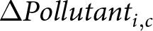 ${{\Delta }}Pollutan{t_{i,c}}$ represents the change in AQI or three pollutants for city
 $c\,$ and pollutant
 $i$;
 ${{\Delta }}Rank{\left( {GDPGR} \right)_{c,2019 - 2022}}$ is the change in GDP growth rankings for city
 $c$ from 2019 to 2022; Xc is a vector of time-varying weather variables such as monthly mean wind speed, rainfall, humidity and temperature;
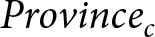 $Provinc{e_c}$ is a dummy variable for province fixed effects;Footnote 3 and
 ${\varepsilon _{i,c}}$ is the random disturbance term. Standard errors are clustered at the province level.
However, as highlighted in the introduction, the change in GDP growth rankings during the COVID-19 period may be endogenous to air pollution due to omitted variables such as government policies, actions of local officials and economic structures. To address this potential endogeneity, we use the number of accumulated infected cases as the IV of growth ranking changes. A key challenge in using this instrument lies in the exclusion restriction, namely whether infection levels could have affected air pollution through channels other than growth rankings. One potential concern is that higher infection counts might have led to stricter lockdowns, reduced mobility and suppressed economic activity, which in turn could have lowered pollution levels. While this channel is theoretically possible, it is unlikely to confound our analysis. Our outcome variable – the change in pollution – is measured for the period 2022–2023, when China had already lifted all COVID-19 control measures, including lockdowns and mobility restrictions. By 2023, both mobility and economic activity had essentially normalized, making it highly improbable that historical infection levels directly influenced pollution outcomes during this subsequent recovery window.
It is also important to recognize that higher infection rates may have temporarily reduced economic activity and pollution during the pandemic years themselves (2020–2022). Such an effect, however, would bias our results in the opposite direction of the mechanism we emphasize. If past infections reduced economic activity, this would induce a negative correlation between the instrument and pollution levels, thereby biasing our IV estimates downward. As a result, our estimates should be viewed as conservative: the true impact of growth-oriented policy responses on pollution may be even larger than reported.
With this identification strategy established, we proceed to estimate the first-stage regression for changes in GDP growth rankings. This regression isolates exogenous variation in relative growth performance driven by the differential impact of COVID-19 across cities, thereby providing a credible basis for our IV approach.
 \begin{equation}\Delta Rank{(GDPGR)_{C,2019 - 2022}} = {\pi _0} + {\pi _1}\log {(AIC)_{C,2019 - 2022}} + \kappa {X_c} + {\lambda }Provinc{e_C} + {\eta _C}\end{equation}
The fitted value of  ${{\Delta }}Rank{\left( {GDPGR} \right)_{c,2019 - 2022}}$ from the first stage in Equation (2) will be used in Equation (1) for the second-stage estimation. Through this two-stage least squares model, we can leverage the exogenous shocks to growth ranking changes caused by AIC to identify the causal impact of growth preference on air pollution. This methodology helps to address potential endogeneity issues, ensuring that the observed relationship is not confounded by other factors. Consequently, we can more accurately attribute changes in air pollution levels to the economic growth preferences of local officials.
The data used in this paper encompasses GDP growth rates, accumulated infected cases, air pollutant concentrations and weather conditions. City-level annual GDP growth data is sourced from various City Statistical Yearbooks, while accumulated infected cases data is obtained from the China Stock Market Accounting Research. AQI and concentrations of air pollutants are sourced from the real-time monitoring platform managed by the China National Environmental Monitoring Centre. Weather data, including daily averages for wind speed, rainfall and temperature, is acquired from the Ministry of Ecology and Environment of China and consolidated into an annual frequency. The meteorological data is taken from the station nearest to the city centre. Additional descriptive statistics for key variables and subsamples are reported in appendix A1.
4. Results
4.1. Main results
Panel A of Table 1 reports OLS estimates on the relationship between changes in GDP growth rankings from 2019 to 2022 and changes in air pollutant concentrations from 2022 to 2023. It shows that changes in GDP growth rankings significantly impact AQI, PM2.5, PM10 and NO2 concentrations. Specifically, a 10-unit change in GDP growth rankings during COVID-19 is associated with increases of 0.04 µg/m3 in AQI, 0.03 µg/m3 in PM2.5, 0.05 µg/m3 in PM10 and 0.03 µg/m3 in NO2 concentrations from 2022 to 2023.
OLS and IV estimates on the effect of growth preference on air pollution

Note: Clustered standard errors in parentheses.
Panel B of Table 1 presents IV estimates of the causal effect of GDP growth ranking changes on air pollutant concentration changes, which are substantially larger (4–9 times) than the OLS estimates in Panel A, indicating significant bias in the OLS estimates. The first stage IV result, shown in column (1), indicates that a 10 per cent increase in accumulated infected cases leads to a 10.169 decrease in GDP growth rankings change from 2019 to 2022, with an F-statistic of 11.16, exceeding the critical value of 10 recommended by Stock et al. (Reference Stock, Wright and Yogo2002) for weak instruments with a single instrument variable. The second stage results in columns (2)–(6) show that a 10-unit change in GDP growth rankings during COVID-19 is associated with increases of 0.26 µg/m3 in AQI, 0.25 µg/m3 in PM2.5, 0.43 µg/m3 in PM10 and 0.014 µg/m3 in NO2 concentrations from 2022 to 2023, which are substantial compared to the average changes in AQI, PM2.5, PM10 and NO2 of 3.727, 1.656, 7.068 and 0.620, respectively (see appendix Table A1). Complementing these causal estimates, appendix Figure A1 presents descriptive evidence on pollution changes across GDP growth ranking groups.
The question that needs to be answered is whether the estimated coefficients of ∆Rank(GDPGR)2019 truly capture the impact of growth preference on pollution, rather than merely a coincidence. To mitigate this concern, we next conduct a falsification test by using other indicators that are not directly related to growth preference. Panel C of Table 1 presents the results of the falsification test by using the change in resident population rankings from 2019 to 2022 as the explanatory variable (∆Rank(POPUGR)2019), contrasting it with the ∆Rank(GDPGR)2019 used in Panel B. The first-stage F-statistics for this estimate are very small, and columns (2)–(6) of Panel C show that the change in resident population rankings during COVID-19 does not have a statistically significant impact on air pollution. This provides strong evidence that the observed effects in Panel B are unlikely to be driven by spurious correlations, further supporting the validity of our main findings regarding the impact of growth preference variation caused by changes in growth rankings during COVID-19 on air pollution changes from 2022 to 2023.
While the above results provide robust evidence on the link between ranking declines and subsequent pollution increases during the pandemic, an important concern is whether the observed changes in rankings simply reflected long-standing structural trends rather than exogenous shocks that triggered policy responses. To further strengthen our identification, we conduct additional analyses.
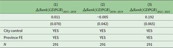
We first test whether the pandemic-induced ranking changes were a continuation of pre-existing dynamics. Specifically, we examine the correlation between ranking changes during the pandemic (2019–2022) and those in the pre-pandemic periods (2015–2018 and 2018–2019). As shown in columns (1) and (2) of Table 2, the estimated correlations are small and statistically insignificant. This finding suggests that the pandemic led to an exogenous ‘reshuffling’ of local growth rankings rather than a simple extension of past trends, thus providing a solid foundation for our natural experiment design.
Correlations between ranking changes across different periods

Note: Clustered standard errors in parentheses.
Next, we provide additional evidence that officials do, in fact, react to these ranking declines by intensifying catch-up efforts. To show that local officials feel pressure and take action in response to a decline in ranking, we examine whether such a decline during the pandemic predicts subsequent catch-up efforts. As shown in column (3) of Table 2, we find that the more a city's ranking dropped during the 2019–2022 period, the more its GDP growth ranking rebounded in 2023. This finding is perfectly consistent with our core narrative: a decline in relative ranking triggers a strong ‘catch-up’ incentive. Our main analysis, in turn, reveals the environmental costs associated with this ‘catch-up’ behaviour.
Taken together, these results provide direct evidence that the pandemic-induced ranking changes were both exogenous and consequential. In China's tournament-style promotion system, a decline in relative ranking serves as a negative performance signal, heightening officials’ career concerns and increasing the marginal return to catch-up effort in the next evaluation cycle. With the nationwide reopening in 2023 relaxing binding constraints, local governments that had fallen behind were able to act on these incentives. Under greater promotion pressure, underperforming cities intensified pro-growth policies with immediate GDP effects – such as infrastructure investment, land supply expansion and industrial stimulus. These measures, by construction, disproportionately stimulate emissions-intensive sectors, thereby linking catch-up growth to higher pollution. Additional robustness analyses, reported in appendix A, confirm that these conclusions remain stable across alternative specifications and samples.
4.2. Mechanism analysis
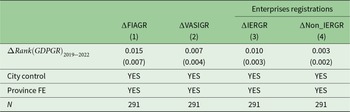
This section discusses several mechanisms through which growth preference may affect air pollution. To explore the strategies employed by local officials, we conduct mechanisms focusing on administrative measures sensitive to governmental influence, including changes in fixed asset investment growth (∆FIAGR), the growth rate of value added in the industrial sector (∆VAISGR) and the growth rate of newly registered industrial enterprises (∆IERGR) from 2022 to 2023. The results using IV estimates are presented in Table 3. To make the coefficients comparable, we standardize the dependent variables by their standard deviation so that the coefficients can be interpreted as how a unit change in growth ranking results in a change measured in standard deviations of the dependent variable.
Mechanisms of growth preference on economic activities

Note: Clustered standard errors in parentheses.
(a) Investment. Local officials frequently use investment as a tool to stimulate economic growth, which has been a cornerstone of the country's economic policy for several decades (Zhu, Reference Zhu2012). We use the growth rate of a city's fixed assets investment to measure the growth stimulating strategy through investment. Column (1) of Table 3 shows a statistically significant positive correlation between ∆FIAGR and ∆Rank(GDPGR)2019. This suggests that cities experiencing a decline in growth ranking tend to stimulate higher levels of fixed asset investment, such as in transportation networks and utilities. However, these large-scale infrastructure projects can lead to environmental consequences, including air pollution from construction activities and increased vehicular emissions.
(b) Industry. Industries, particularly those related to infrastructure and manufacturing, are generally more affected by local governments’ stimulating policies than other sectors. Also, industries usually receive significant attention and support from government stimulus measures. In this paper, we use the growth rate of a city's value added of the secondary industry to measure local officials’ emphasis on industries for encouraging growth. Column (2) of Table 3 demonstrates a significant positive correlation between ∆VAISGR and ∆Rank(GDPGR)2019, indicating that cities shocked more by the COVID pandemic and which thus experienced a decline in growth ranking tend to encourage the industrial sector. However, industries are primarily more pollution-intensive, which may contribute to air pollution through factory emissions.
(c) Easing the registration requirements for more polluting companies. This can provide short-term economic benefits because of quick boosts to the economy by increasing industrial production, construction activities and related economic activities. Since industrial companies are usually more pollution intensive, we use the growth rate of city's industrial enterprise registrations to measure the registration requirements for more polluting companies. Column (3) of Table 3 indicates a significant positive association between ∆IERGR and ∆Rank(GDPGR)2019. Interestingly, when we turn to the registration of non-industrial enterprises (∆Non_IERGR), the result in column (4) of Table 3 reveals a lack of statistical significance in the relationship between change in the non-industrial enterprises and change in GDP growth rankings.
4.3. Excluding alternative explanations
(a) Not an effect of economic recovery. Cities significantly affected by the pandemic experienced substantial declines in growth rankings from 2020 to 2022. A potential alternative explanation for the subsequent pollution increase in 2023 is that it merely reflects a mechanical economic rebound. If this were the case, pollution levels should be expected to return to their pre-pandemic baseline of 2019, but not to exceed it. To directly test this hypothesis, we use the 4-year change in pollution (2019–2023) as the outcome variable. The results, presented in Table 4, provide strong evidence against the simple rebound story and instead offer nuanced support for our main conclusions.
Excluding alternative explanation: economic recovery (using 2019–2023 pollution changes as the outcome)

Note: Clustered standard errors in parentheses.
First, the results rule out a simple rebound to baseline. The core of the rebound hypothesis is that pollution in 2023 would simply return to its 2019 level. If this were true, the coefficients on our variable of interest should be close to zero. However, as shown in Table 4, the IV point estimates for the effect of a GDP ranking decline are consistently positive across all four pollutants (0.149 for AQI, 0.116 for PM2.5, 0.208 for PM10 and 0.096 for NO2). This indicates that in cities where officials had stronger incentives for growth, pollution levels in 2023 did not just recover to the 2019 baseline, but in fact overshot it. This is perfectly aligned with our hypothesis.
Second, statistical power is expectedly lower, but the overall pattern of evidence remains strong. We acknowledge that the point estimates do not reach statistical significance using conventional t-statistics. This is expected due to the nature of the long-difference (2019–2023) outcome variable. This 4-year window aggregates two large, opposing effects: a pollution decrease during the 2020–2022 lockdown period followed by a pollution increase during the 2023 recovery. This ‘dip-and-rebound’ dynamic naturally increases the variance of the outcome variable, which reduces the statistical power of the test and makes precise estimation more challenging.
Third and crucially, inference based on the Anderson–Rubin (AR) confidence intervals provides robust evidence. Given the potential for reduced power, we turn to the AR confidence intervals, which provide valid inference. For PM2.5, the most closely watched pollutant for health impacts, the 95 per cent AR confidence interval is [0.1, 0.45]. As this interval is strictly positive and does not contain zero, it provides statistically robust evidence that a decline in GDP ranking led to a significant increase in PM2.5 pollution over and above the pre-pandemic baseline. Furthermore, the AR intervals for the other pollutants strongly corroborate this finding. For instance, the intervals for AQI ([−0.02, 0.57]), PM10 ([−0.01, 0.74]) and NO2 ([−0.01, 0.34]) are all overwhelmingly concentrated in the positive range, with zero being only marginally included at the lower bound. This consistent pattern across all key pollutants reinforces the conclusion that the underlying effect is positive and not an artefact of random noise.
Overall, the evidence decisively rules out a simple rebound explanation. Instead, it underscores the role of policy-driven responses to ranking declines, which pushed pollution in 2023 beyond pre-pandemic levels. This finding further reinforces our central claim that local officials’ catch-up strategies, rather than mechanical recovery dynamics, account for the observed increase in pollution.
(b) Not an effect of overtime working. Another possible explanation is that companies in cities more impacted by the COVID-19 pandemic might bear a heavier burden in recovering. These challenges can include increased financial strain, disrupted supply chains and the need to restore operations and workforce stability. Consequently, these companies may require employees to work overtime to meet recovery targets, compensate for lost productivity and accelerate their return to pre-pandemic performance levels. This overtime work is also related to increased pollutant emissions. If this is the case, the observed effect on air pollution would result from overtime work rather than the growth preferences of local officials.
To test this hypothesis, we use changes in satellite night-time light data as an indicator of changes in overtime work hours, as proposed by Li et al. (Reference Li, Tu, Tong, Cao, Zhong, Zhang, Zhu and Li2024). This approach allows us to determine whether regions experiencing a decline in GDP rankings following the pandemic show increased levels of overtime work, potentially contributing to higher pollution levels. Table 5 using IV estimate shows no statistically significant association. This suggests that the strategies adopted by local officials to enhance GDP rankings post-pandemic do not necessarily translate into increased working intensity among enterprises.
Excluding alternative explanation: overtime working

Note: Clustered standard errors in parentheses.
5. Further discussion: a rational course of action for local officials
The empirical analyses indicate that local officials in China, responding to growth preferences linked to GDP, may have motivation to improve their rankings after the COVID-19 pandemic with various strategies including less stringent environmental regulations. This policy shift has led to a degradation of air quality. While economic growth remains crucial, environmental performance is also a key metric for evaluating local government officials, though it is weighted less heavily than economic metrics (Wu and Cao, Reference Wu and Cao2021). Thus, a rational course of action for multitasking local officials would be to relax environmental regulations just enough to meet minimum air quality control targets while promoting economic growth, which is closely tied to their career prospects (Cao et al., Reference Cao, Weng, Xu and Zhou2021).
To investigate this hypothesis further, we conduct additional research within this multitasking context in China. Central or provincial governments assign city-level air pollution targets, typically specifying a minimum number of days with good or moderate air quality (AQI ≤ 100). We manually collected data on these targets and their fulfilment status for each city, allowing us to create a variable indicating whether the 2023 air quality improvement targets were achieved (1 for met, 0 for not met). The data shows that 72.2 per cent of cities successfully met their air pollution control targets (see appendix Table A1).
Using this binary variable as the dependent variable, we conduct both IV regression and OLS regression. The results, presented in Table 6, show that neither regression produced statistically significant results. These non-significant coefficients suggest that although variations in growth preference due to changes in growth rankings affect air pollution, local officials are rational enough to meet the minimum air quality control targets included in the checklist of officials’ promotion criteria.
Effect of growth preference on achieving minimum air quality control targets

Note: Clustered standard errors in parentheses.
6. Conclusions
Preference is one of the most important elements in economists’ conceptual framework driving human behaviours. Building on extensive surveys, Falk et al. (Reference Falk, Becker, Dohmen, Enke, Huffman and Sunde2018) posit that variations in preferences are correlated with behaviours and economic outcomes. This paper investigates the impacts of growth preference on environmental outcomes and the underlying mechanisms using city-level data from China.
Given that Chinese local officials link their promotion prospects to the relative performance of local economic growth compared to their peers, we use changes in GDP growth rankings to capture variations in growth preference. To precisely estimate the impacts, we leverage the GDP shuffling caused by COVID-19, which resulted in unprecedented and uneven economic disruptions across cities. We find that a 10-unit change in GDP growth rankings, all else being equal, increases the AQI by 0.26, PM2.5 by 0.25 µg/m3, PM10 by 0.43 µg/m3 and NO2 by 0.14 µg/m3 in the IV estimates. These findings are robust to alternative specifications.
We identify three powerful predictors that drive environmental consequences: fixed investments, industrial activities and registration requirements for more polluting companies. Perhaps the most policy-relevant is the fact that all these factors are sensitive to governmental influence, with fixed investment showing the most significant effect. This aligns with China's long-standing economic policy focus.
We also exclude competing explanations related to natural economic recovery after a depression and overtime working incentives of companies for recovery targets, ensuring that the discrepancy in air pollution is attributed to the growth preferences of local officials.
Furthermore, we examine the cautious behaviours of local officials in balancing economic and environmental objectives. Despite increased average air pollution levels, officials meet minimum air quality control targets to avoid jeopardizing their career prospects. This multitasking context highlights the trade-offs faced by officials who must prioritize local GDP growth while adhering to environmental standards. This suggests policy interventions considering the dual objectives of economic growth and environmental protection. Strengthening environmental regulations and aligning them with promotion criteria could mitigate the adverse effects of growth preferences on air quality.
Supplementary material
The supplementary material for this article can be found at https://doi.org/10.1017/S1355770X26100497.
Acknowledgements
The authors acknowledge support from the National Natural Science Foundation of China (Grant no. 72173095), Key Project of Social Science in China and Major Project of Social Science in China.
Competing interests
The authors declare that there are no conflicts of interest, we do not have any possible conflicts of interest.
AI
During the preparation of this manuscript, the authors used the AI-assisted tool ChatGPT (developed by OpenAI) for the purpose of language editing and polishing. The use of this tool was limited to improving grammar, syntax and clarity. The authors reviewed and edited all AI-generated suggestions and take full responsibility for the final content of the manuscript.