1 Introduction
In offshore engineering, different kinds of cylindrical structures are widely encountered. Good understanding of the flow around these structures is key to safe and optimal designs. As an extensively studied and well-documented topic, flow around a straight circular cylinder has served as a basis to understand more complicated cylindrical structure wake flows (Zdravkovich Reference Zdravkovich1997; Sumer & Fredsøe Reference Sumer and Fredsøe2006). However, flow behind different configurations, e.g. inclined cylinder, curved cylinder, etc., all have their own special features that need to be investigated independently. Among these configurations, curved cylinders have received increasing attention recently.
1.1 The curved cylinder wake
Curved cylinders are commonly adopted in pipelines lying on the seabed to transport oil and gas, as well as in catenary risers in the ocean space between the free surface and connections to the sea floor. Despite the fact that a curved cylinder is easy to define, design and construct, the flow around it in the ocean space is very complicated, leading to complex hydrodynamic forces and multiple frequencies, which have not yet been well addressed in the literature. To the authors’ knowledge, there is still a lack of effective guidelines to design the curved parts of offshore cylindrical structures. As a result, excessive safety factors are often used in the design phase to ensure the reliability of these structures. A comprehensive and good understanding of the curved cylinder wake is therefore not only an interesting fluid mechanics topic, but also a practical engineering topic.
Earlier studies of curved cylinder wakes mostly focused on flow normal to the plane of curvature, essentially the flow past a ring structure, as reviewed by Gallardo, Pettersen & Andersson (Reference Gallardo, Pettersen and Andersson2014a
). Miliou et al. (Reference Miliou, de Vecchi, Sherwin and Graham2007) were among the first to carry out detailed curved cylinder wake studies in which the flow is directed in the plane of curvature. They conducted a three-dimensional (3-D) direct numerical simulation (DNS) study of the curved cylinder wake at Reynolds numbers
 $Re\leqslant 500$
, where the flow is not yet turbulent. De Vecchi, Sherwin & Graham (Reference de Vecchi, Sherwin and Graham2008) conducted a 3-D numerical study of curved cylinder wakes at
 $Re=100$
, and considered both stationary and forced oscillating geometries. Assi et al. (Reference Assi, Srinil, Freire and Korkischko2014) conducted experimental observations of a stationary curved cylinder wake at
 $Re=1000$
. Miliou et al. (Reference Miliou, de Vecchi, Sherwin and Graham2007), de Vecchi et al. (Reference de Vecchi, Sherwin and Graham2008) and Assi et al. (Reference Assi, Srinil, Freire and Korkischko2014) all considered two configurations, i.e. the convex curved cylinder, when the inflow is towards the outer face of the curvature, and the concave curved cylinder, when the inflow is reversed. The main features of the two configurations turn out to be distinctly different.
Gallardo et al. (Reference Gallardo, Pettersen and Andersson2014a
) and Gallardo, Pettersen & Andersson (Reference Gallardo, Pettersen and Andersson2014b
) carried out the first 3-D DNS study of the turbulent wake behind a convex curved cylinder at
 $Re=3900$
, where detailed wake dynamics analysis as well as proper orthogonal decomposition (POD) analysis of the wake were presented. The choice of boundary conditions for the convex curved cylinder simulations was also studied by the same authors (Gallardo, Pettersen & Andersson Reference Gallardo, Pettersen and Andersson2013).
The concave curved cylinder wake is, on the other hand, significantly different and more complex compared to the convex one. The opposite flow direction induces a strong axial flow behind the curved part of the cylinder, and suppresses the vortex shedding in the wake. This was first pointed out by Miliou et al. (Reference Miliou, de Vecchi, Sherwin and Graham2007). However, it was not until more recently that the concave curved cylinder wake was investigated in depth and more interesting wake phenomena were revealed.
Shang, Stone & Smits (Reference Shang, Stone and Smits2018) conducted a series of experimental visualizations on both convex and concave curved cylinder wakes at
 $Re\leqslant 916$
, and focused mostly on the concave configuration. They discovered coexisting flow regimes in the concave curved cylinder wake similar to what was proposed for the inclined cylinder wake by Ramberg (Reference Ramberg1983), namely two non-shedding regimes and two shedding regimes. Shang et al. (Reference Shang, Stone and Smits2018) pointed out that the axial flow that developed from the curved part of the cylinder induced strong streamwise vorticity such that the oblique shedding angle behind a concave curved cylinder can be rather high (typically
 $40^{\circ }$
–
 $45^{\circ }$
). They also considered different curvatures and different aspect ratios (ratio between the arclength of the curved cylinder and the cylinder diameter), and therefore presented a parameter study. In their experimental investigation, free cylinder end and free surface effects were present.
Jiang, Pettersen & Andersson (Reference Jiang, Pettersen and Andersson2018a
) and Jiang et al. (Reference Jiang, Pettersen, Andersson, Kim and Kim2018b
) conducted 3-D numerical studies on the concave curved cylinder wake by means of DNS. Different from the experimental set-ups, they appended straight extensions at both the vertical and horizontal ends of the concave curved cylinder, such that no free ends were present in the flow field. By means of a series of DNS, they investigated the length effect of both the horizontal and vertical extensions, as well as the main features of this wake flow at low
 $Re\leqslant 500$
. Jiang et al. (Reference Jiang, Pettersen, Andersson, Kim and Kim2018b
) also reported the existence of multiple flow regimes in the concave curved cylinder wake, which agrees with the experimental observations in Shang et al. (Reference Shang, Stone and Smits2018). As an advantage in numerical set-ups, Jiang et al. (Reference Jiang, Pettersen, Andersson, Kim and Kim2018b
) could freely vary the vertical extension length. This further allowed them to study the frequency variation along the curved cylinder span, and revealed various types of frequency variation over a relatively small
 $Re$
range.
Zhu et al. (Reference Zhu, Bao, Zhou and Wang2017, Reference Zhu, Zhou, Bao, Wang, Lu, Fan and Han2018, Reference Zhu, Wang, Bao, Zhou, Ping, Han and Sherwin2019) considered a catenary shaped curved circular cylinder, namely the combination of a convex and a concave curved cylinder, and studied the wake behind this configuration at
 $Re\leqslant 100$
. The focus of their studies was to compare how the wake is influenced when the inflow direction is changed. Therefore, in their studies, the incoming flow is not only confined to the plane of curvature. Moreover, due to the presence of both the concave and convex curved parts simultaneously (and sometimes close to each other), the wake interactions make this flow a more complicated case. Jung et al. (Reference Jung, Oh, Nam, Park, Kwon and Jung2019) conducted 3-D numerical simulations of flows around a curved circular cylinder with different inflow directions at
 $Re=100$
.
In addition to the above-mentioned curved cylinder wake studies, where the cylinder is kept stationary, vortex-induced vibration (VIV) of curved cylinder configurations is also of great interest, motivated by elastic catenary risers. Most VIV studies with curved cylinder configurations are experimental (see de Vecchi, Sherwin & Graham (Reference de Vecchi, Sherwin and Graham2009), Srinil (Reference Srinil2010), Assi et al. (Reference Assi, Srinil, Freire and Korkischko2014) and Srinil, Ma & Zhang (Reference Srinil, Ma and Zhang2018), and the studies mentioned therein). Such VIV problems are close to real engineering applications, and the focus of these studies has mainly been on hydrodynamic force coefficients and motions. Nevertheless, the physical understanding gained from stationary curved cylinder wake studies serves as the basis for VIV studies mentioned here. However, VIV is beyond the scope of the present study.
From this review of the literature on the curved cylinder wake, it is clear that the present configuration has received increasing attention in recent years. Understanding of the wake behind curved cylinders, especially behind a concave curved cylinder, is still far from comprehensive. Most studies are still at relatively low Reynolds numbers (
 $Re\leqslant 1000$
), and there is clearly a great demand for more investigations into this topic.
1.2 Straight circular cylinder wake at
 $Re=3900$

Wake flow behind a straight circular cylinder at various
 $Re$
has been one of the most classic topics in the fluid mechanics community. The literature on this topic is rich and we do not aim to give a comprehensive review. Yet, since the Reynolds number (3900) that we consider here has emerged as a preferred
 $Re$
for circular cylinder wake studies, we would like to briefly summarize some of these studies as a background for our investigation.
Three transition processes take place successively as the circular cylinder wake gradually turns from laminar to fully turbulent, i.e. wake transition, shear layer transition and boundary layer transition. They are dominated by distinct instabilities and have become independent research topics. Reynolds number
 $Re=3900$
is in the shear layer transition process where Kelvin–Helmholtz instabilities take place in the shear layers separating from the cylinder.
Early studies that paid particular attention to
 $Re=3900$
are by Beaudan & Moin (Reference Beaudan and Moin1994), Lin, Towfighi & Rockwell (Reference Lin, Towfighi and Rockwell1995), Ong & Wallace (Reference Ong and Wallace1999), among others. Following these studies, there emerged a wealth of research at this
 $Re$
, for example by Kravchenko & Moin (Reference Kravchenko and Moin2000), Ma, Karamanos & Karniadakis (Reference Ma, Karamanos and Karniadakis2000), Dong et al. (Reference Dong, Karniadakis, Ekmekci and Rockwell2006) and Parnaudeau et al. (Reference Parnaudeau, Carlier, Heitz and Lamballais2008), to mention only a few. Owing to the fruitful results obtained from numerous studies, the circular cylinder wake at
 $Re=3900$
evolved as a standard benchmark case for the validation of different numerical methods (e.g. Mahesh, Constantinescu & Moin Reference Mahesh, Constantinescu and Moin2004; Jacob, Malaspinas & Sagaut Reference Jacob, Malaspinas and Sagaut2018). Interested readers are recommended to consult the good reviews by Kravchenko & Moin (Reference Kravchenko and Moin2000) and Parnaudeau et al. (Reference Parnaudeau, Carlier, Heitz and Lamballais2008).
Zdravkovich (Reference Zdravkovich1997) divided the shear layer transition of a circular cylinder wake into three stages, namely the early stage TrSL1 (
 $350<Re<2000$
), the intermediate stage TrSL2 (
 $2000<Re<40\,000$
) and the late stage TrSL3 (
 $40\,000<Re<200\,000$
). The borders between these stages are not precisely clear. Generally speaking,
 $Re=3900$
falls into stage TrSL2, in which the wake is turbulent, the shear layers just start to form Kelvin–Helmholtz vortices and are not yet turbulent, and the boundary layer is still laminar. This means that, at
 $Re=3900$
, one should expect to see rather stable and elongated free shear layers on both sides of the cylinder. A typical example of a circular cylinder wake at
 $Re=3900$
can be found in figure 4 of Parnaudeau et al. (Reference Parnaudeau, Carlier, Heitz and Lamballais2008).
1.3 Other relevant cylindrical structures
For a curved cylinder, continuous variations of some geometric parameters appear along its span, such as varying elliptic horizontal cross-sections, varying local tangential direction (or angle of attack), etc. These variations give rise to a spanwise non-uniformity along the cylinder, which will apparently influence the flow physics in the wake. Studying these influences will not only improve our understanding of curved cylinder wakes, but also help us make connections to similar wake physics behind other cylinder configurations. It therefore becomes interesting to draw some analogies between the concave curved cylinder wake and wakes behind other cylindrical structures. One straightforward varying geometric parameter is the horizontal elliptic cross-section, for which the analogy with a straight elliptic cylinder could be made. Compared to the circular cylinder wake, the elliptic cylinder wake has received less attention – see e.g. the introductions in Leontini, Jacono & Thompson (Reference Leontini, Jacono and Thompson2015) and Paul et al. (Reference Paul, Prakash, Vengadesan and Pulletikurthi2016). Depending on whether the major or the minor axis of the ellipse is aligned with the incoming flow, an elliptic cylinder can appear either more slender or more bluff compared to a circular cylinder, leading to different flow features. In the concave curved cylinder configuration, despite the varying aspect ratio of the elliptic cross-section, the major axis is always aligned with the inflow. Therefore, we only need to consider possible similarities between more slender elliptic cylinder wakes and the present wake. If the elliptic cross-section analogy is valid, we should expect a narrower wake and higher shedding frequency behind the concave curved cylinder as compared to those behind a circular cylinder at the same
 $Re$
, as shown in Shirakashi, Hasegawa & Wakiya (Reference Shirakashi, Hasegawa and Wakiya1986) and commented upon by Zdravkovich (Reference Zdravkovich1997, § 25.3.2).
The varying axial direction along the curved cylinder span, or equivalently the varying local attack angle of the incoming flow, encourages us to consider a possible analogy between the concave curved cylinder wake and an inclined straight circular cylinder (also referred to as a yawed cylinder) wake. The inclined cylinder wake is popular especially in the aerodynamic community due to its similarity to a manoeuvring aircraft. It has been extensively investigated (e.g. by Ramberg (Reference Ramberg1983), Snarski (Reference Snarski2004), Zhao, Cheng & Zhou (Reference Zhao, Cheng and Zhou2009) and Ma & Yin (Reference Ma and Yin2018), and the many other studies mentioned therein). The features of the inclined cylinder wake are highly dependent on the angle of attack. As the angle of attack increases from
 $0^{\circ }$
(i.e. cylinder axis aligned with inflow) to
 $90^{\circ }$
, the inclined cylinder wake is usually classified into four types: attached flow, symmetric vortices, steady asymmetric vortices and unsteady vortex shedding (Zdravkovich Reference Zdravkovich1997; Ma & Yin Reference Ma and Yin2018). Steady asymmetric vortices that appear at medium high attack angles are most representative. Asymmetric helical vortices are, in this case, generated alternately along the cylinder span, and stay at almost fixed positions, as was nicely visualized by Thomson & Morrison (Reference Thomson and Morrison1971). If an analogy with the inclined cylinder is valid, we should expect to observe all four types of flow coexisting in the present wake along the curved cylinder span.
Another possible analogy is between the present wake and the wake behind a circular cylinder with a splitter plate. This is based on previous observations that there exists a strong axial flow behind the concave curved cylinder (Miliou et al.
Reference Miliou, de Vecchi, Sherwin and Graham2007; Jiang et al.
Reference Jiang, Pettersen, Andersson, Kim and Kim2018b
; Shang et al.
Reference Shang, Stone and Smits2018). Jiang et al. (Reference Jiang, Pettersen, Andersson, Kim and Kim2018b
) showed that the magnitude of the axial velocity behind a concave curved cylinder can be comparable to the inflow velocity, at
 $Re\leqslant 500$
. Such prominent axial flow may prevent the interaction between the free shear layers shed from the two sides of the cylinder and act equivalently to a splitter plate. A recent study on the wake behind a circular cylinder with splitter plate (Serson et al.
Reference Serson, Meneghini, Carmo, Volpe and Gioria2014) provides a review of relevant references on this topic. Generally speaking, with a splitter plate appended behind the cylinder, due to the interruption of shear layer interactions, the recirculation region is longer and the shedding frequency is lower.
In this paper, we will bear these analogies in mind when we present our observations.
1.4 Objectives of the present study
The above review shows that the concave curved cylinder wake is diverse and has some atypical, yet interesting, flow features, e.g. coexisting flow regimes, strong dislocations, etc. So far, our understanding of this wake flow has been restricted to studies at low Reynolds numbers. There is clearly a lack of a comprehensive investigation on the turbulent wake behind this configuration, which becomes the primary scope of this study. The Reynolds number considered in the present paper is
 $Re=3900$
.
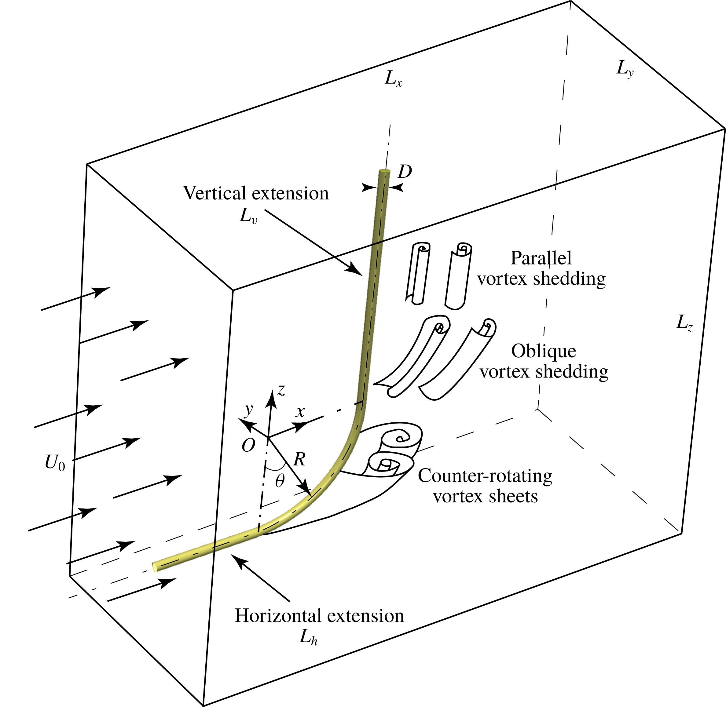
Configuration of the flow problem and definition of the coordinate system and origin. The not-to-scale 3-D computational domain as well as a not-to-scale sketch of the main features of this wake are also included.

We choose DNS as the numerical tool for two reasons. First, DNS is currently the most reliable computational fluid dynamics (CFD) tool that provides detailed flow data for physical analysis. Second, the counter-rotating vortex sheet pair, which dominates a substantial wake region behind the curvature, as sketched in figure 1, is rather stable. We could anticipate it to stay laminar over a wide
 $Re$
range. This intrinsic characteristic may make this flow challenging for other numerical approaches, especially Reynolds-averaged Navier–Stokes (RANS) methods. It is most likely that laminar flow, turbulent flow, and even a transition between them, will occur simultaneously in the wake.
Before the dynamics in the wake are investigated, we will present two computational topics: the grid study and the vertical extension study. The vertical extension study is an important computational issue for the concave curved cylinder flow simulations. Jiang et al. (Reference Jiang, Pettersen, Andersson, Kim and Kim2018b
) demonstrated that an inadequate vertical extension length (
 $L_{v}$
; see figure 1) limits the space for proper development of the oblique shedding behind the straight part, and consequently influences the lower part of the wake (i.e. that behind the curved cylinder). A general trend is that the effect of
 $L_{v}$
is reduced as
 $Re$
increases (see figure 11 in Jiang et al. (Reference Jiang, Pettersen, Andersson, Kim and Kim2018b
)), which is favourable for higher-
 $Re$
DNS on account of the computational cost. However, there is no a priori experience on the
 $L_{v}$
effect at
 $Re=3900$
. Therefore, a vertical extension study is essential in view of both efficiency and rigorousness.
After the computational issues are addressed, we will discuss the wake dynamics from different aspects. Coexisting flow regimes and complex vortex dislocations will be documented first, followed by discussions about new observations on the axial flow close behind the cylinder. Distinct flow dynamics will be presented in detail with connection to frequency components, before an overall perspective of the whole wake can be outlined. At last, the earlier-mentioned cylinder geometry analogies will be addressed.
2 Mathematical modelling and computational issues
2.1 Flow configuration
We consider a quarter-ring curved cylinder with straight extensions appended to both of its ends. The diameter of the cylinder is denoted
 $D$
. The radius of the ring, i.e. radius of the centreline of the curved part of the cylinder, is
 $R=12.5D$
. A perspective view of the geometry, together with a not-to-scale sketch of the computational domain, is shown in figure 1. The main features of this wake flow, as learned from earlier low-
 $Re$
investigations (see Jiang et al.
Reference Jiang, Pettersen, Andersson, Kim and Kim2018b
; Shang et al.
Reference Shang, Stone and Smits2018) are also sketched. The Reynolds number
 $Re$
is defined based on the free-stream velocity
 $U_{0}$
and cylinder diameter
 $D$
, i.e.
 $Re=U_{0}D/\unicode[STIX]{x1D708}$
, where
 $\unicode[STIX]{x1D708}$
is the kinematic fluid viscosity.
The coordinate system is defined with
 $x$
in the streamwise direction,
 $y$
in the cross-flow direction and
 $z$
in the vertical direction. The origin
 $O$
of the coordinate system is at the centre of curvature (see figure 1). The computational domain has lengths
 $L_{x}$
,
 $L_{y}$
and
 $L_{z}$
in the corresponding directions. In order to eliminate the free-end effects in the simulations, we append straight extensions at both ends of the curved part. They are referred to as vertical extension and horizontal extension, and their lengths are denoted
 $L_{v}$
and
 $L_{h}$
, respectively. Both extensions are important for the present configuration, as discussed by Jiang et al. (Reference Jiang, Pettersen, Andersson, Kim and Kim2018b
). Moreover, both the straight extensions have a clear real-life significance, because curved cylinder structures, as a part of either a catenary riser or a deep-sea pipeline, never appear isolated.
2.2 Governing equations and boundary conditions
In a DNS study, the governing equations are the mass conservation equation (2.1) and the time-dependent 3-D full Navier–Stokes (N–S) equation (2.2) for incompressible flows:
 $$\begin{eqnarray}\displaystyle & \unicode[STIX]{x1D735}\boldsymbol{\cdot }\boldsymbol{u}=0, & \displaystyle\end{eqnarray}$$
 $$\begin{eqnarray}\displaystyle & \displaystyle \frac{\unicode[STIX]{x2202}\boldsymbol{u}}{\unicode[STIX]{x2202}t}+(\boldsymbol{u}\boldsymbol{\cdot }\unicode[STIX]{x1D735})\boldsymbol{u}=\unicode[STIX]{x1D708}\unicode[STIX]{x1D6FB}^{2}\boldsymbol{u}-\frac{1}{\unicode[STIX]{x1D70C}}\unicode[STIX]{x1D735}p. & \displaystyle\end{eqnarray}$$
Here
 $\unicode[STIX]{x1D70C}$
denotes the constant fluid density, and
 $\unicode[STIX]{x1D735}$
is the gradient operator. The gravity force is omitted in (2.2). We apply the following boundary conditions in the simulations.
(i) At the inlet: uniform incoming velocity
$\boldsymbol{u}=(u,v,w)=(U_{0},0,0)$
.(ii) At the outlet: Neumann boundary condition
$(\unicode[STIX]{x2202}u/\unicode[STIX]{x2202}x=\unicode[STIX]{x2202}v/\unicode[STIX]{x2202}x=\unicode[STIX]{x2202}w/\unicode[STIX]{x2202}x=0)$
and zero pressure (
$p=0$
).(iii) At the other four boundaries of the domain: free-slip boundary conditions.
(iv) At the surface of the cylinder: no-slip and impermeability wall boundary condition.



2.3 Numerical methods
The governing equations (2.1) and (2.2) are directly solved without introducing any turbulence model. A well-verified second-order finite-volume direct numerical simulation/large-eddy simulation (DNS/LES) code MGLET (Manhart, Tremblay & Friedrich Reference Manhart, Tremblay, Friedrich, Jenssen, Kvamsdal, Andersson, Pettersen, Ecer, Periaux, Satofuka and Fox2001) is utilized to conduct all the simulations. In MGLET, equations (2.1) and (2.2) are discretized on a 3-D staggered Cartesian mesh. The discretized equations are integrated in time with Williamson’s third-order low-storage Runge–Kutta scheme (Williamson Reference Williamson1980), while pressure corrections are achieved by Stone’s strongly implicit procedure (SIP) (Stone Reference Stone1968). The representation of the cylindrical geometry inside the Cartesian mesh is accomplished by a direct-forcing immersed boundary method (IBM). The details of this IBM implementation and its validation can be found in Peller et al. (Reference Peller, Le Duc, Tremblay and Manhart2006). The code has recently been used for DNS/LES of the same curved cylinder configuration (Jiang et al. Reference Jiang, Pettersen, Andersson, Kim and Kim2018b ) as well as various other flow configurations (e.g. Gallardo et al. Reference Gallardo, Pettersen and Andersson2014a ; Tian et al. Reference Tian, Jiang, Pettersen and Andersson2017; Strandenes et al. Reference Strandenes, Jiang, Pettersen and Andersson2019).
MGLET uses a multi-level 3-D Cartesian mesh, and mesh generation is based on a zonal grid algorithm (Manhart Reference Manhart2004). The overall mesh consists of various numbers of cubic grid boxes (grids) at different levels. Each grid consists of
 $N\times N\times N$
uniform Cartesian cells, regardless of the size of the grid. In other words, every single cell has an ideal aspect ratio of 1 : 1 : 1. The grids are otherwise distributed in an unstructured manner, such that local refinement can be achieved with the zonal grid algorithm. For each refinement, the parent-level grid is split into eight equal child-level grids. Normally, the most-refined cells are applied to regions of interest, because full DNS resolution over the whole computational domain is unaffordable in wake simulations. The regions of interest are selected based on certain criteria, both manually and automatically. For the present simulations, we ensure that all regions with time-averaged vorticity magnitude above
 $0.1U_{0}/D$
are refined (automatically). In addition, the near wake (including the boundary layers) is resolved with DNS resolution down to
 $x/D=16.5$
, and with the second finest resolution down to
 $x/D\approx 23.5$
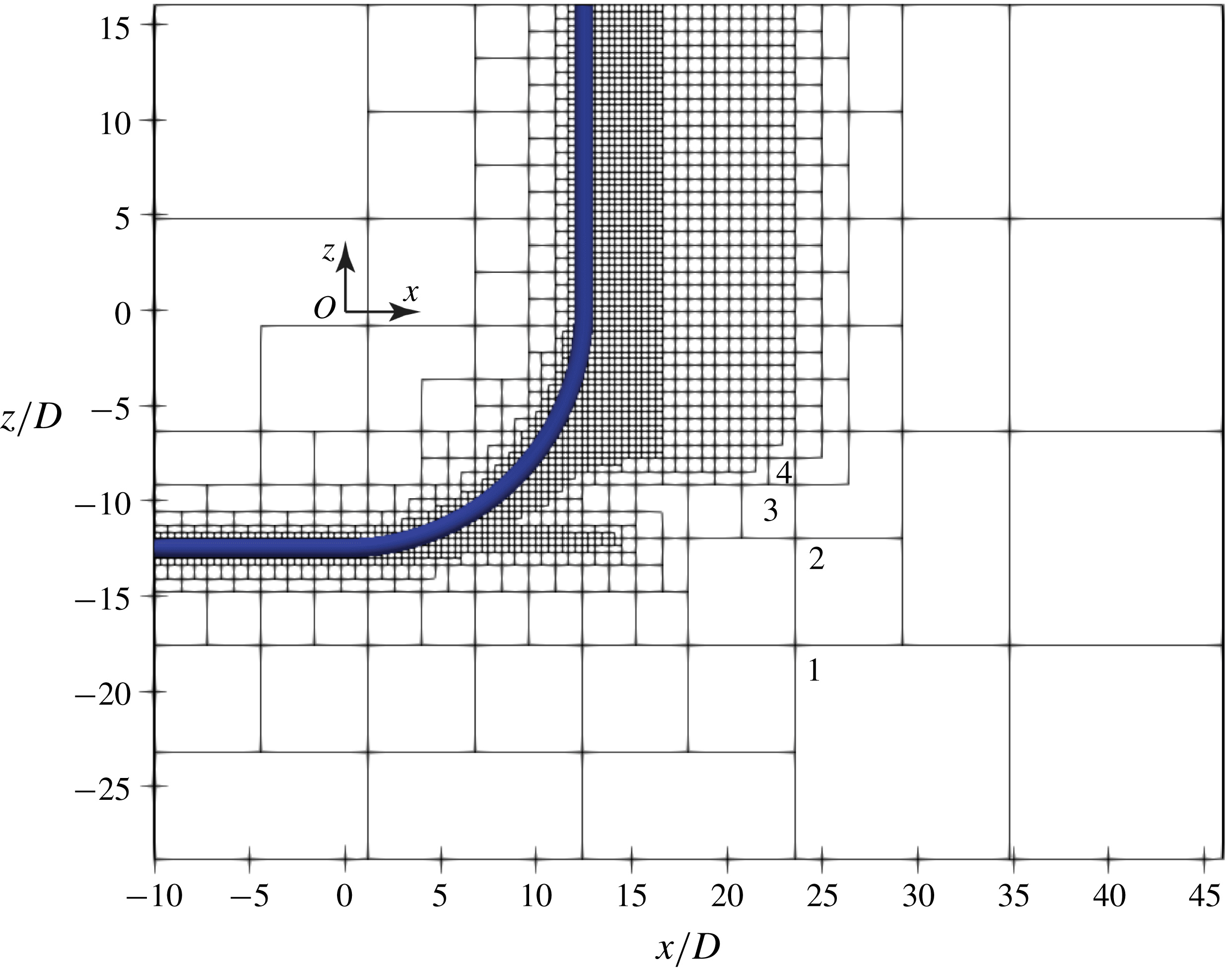
(manually fixed). This mesh generation method offers the possibility to refine only the flow regions of interest without sacrificing either grid quality or wasting any cells. A slice of the mesh structure of case VE-16D taken in the geometrical symmetry plane (the
 $(x,z)$
-plane at
 $y/D=0$
) is shown in figure 2 to illustrate the zonal grid algorithm.
A slice of the VE-16D mesh (see table 1) in the symmetry plane. Each square represents one grid box that consists of
 $N\times N\times N$
uniform Cartesian cells, regardless of its size. The coarsest four levels (out of in total six levels) of grids are marked with numbers.

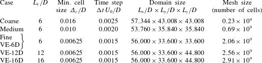
Mesh parameters of all simulations in the present study. The mesh for case Fine and case VE-6D is the same. It is used for both the grid study and the vertical extension study, and therefore has two labels to ease the discussions. The case Coarse has five levels of grids, and the other cases all have six levels of grids. For all cases in this table,
 $Re=3900$
and
 $L_{h}/D=10$
. From the data in this table, one sees that the largest blockage in the
 $y$
direction is less than 3 %.
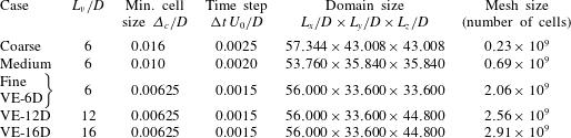
In table 1, we summarize the computational parameters of all simulations in the present study. Five DNS are required to address two computational issues: grid study with cases Coarse, Medium and Fine, and vertical extension study with cases VE-6D, VE-12D and VE-16D. The mesh for case Fine is also used in the vertical extension study (VE-6D) and therefore has two different labels for the convenience of discussions. In-depth investigations of the wake dynamics will be based on the results from case VE-16D. In all simulations, the time step
 $\unicode[STIX]{x0394}t$
is chosen to ensure that the maximum Courant–Friedrichs–Lewy (CFL) number is smaller than 0.5. It is worth mentioning that the (multi-level) mesh topology of Coarse, Medium and Fine meshes are kept the same, but the minimum cell size
 $\unicode[STIX]{x1D6E5}_{c}/D$
is varied to consider different resolutions in the grid convergence study.
2.4 Grid convergence and statistical convergence
Although it is difficult to find directly comparable experimental results for the present configuration in the literature, we did careful validations on straight circular cylinder flows with the same code. These comparisons were presented in Gallardo et al. (Reference Gallardo, Pettersen and Andersson2014a ) and Strandenes et al. (Reference Strandenes, Pettersen, Andersson and Manhart2017), for example, and serve as a good basis for the present work. We still need a systematic mesh study.
Three meshes with different grid resolutions (
 $\unicode[STIX]{x1D6E5}_{c}/D$
) were considered to investigate grid convergence, all with the shortest vertical extension
 $L_{v}/D=6$
. One notices that the domain size is not fixed for the three grid study simulations, because
 $L_{x}$
,
 $L_{y}$
and
 $L_{z}$
are not necessarily integers in our mesh generation strategy. On the other hand, they must fit to an integer multiple of the edge length of the coarsest grid box, i.e. following
 $$\begin{eqnarray}L_{i}=\text{integer}\times N\times \unicode[STIX]{x1D6E5}_{c}\times 2^{N_{L}-1},\quad i=x,y,z,\end{eqnarray}$$
where
 $N$
is the number of cells on one edge of the grid box,
 $N_{L}$
is the level of grids in a mesh and
 $\unicode[STIX]{x1D6E5}_{c}$
is the minimum grid cell size. The case Coarse has
 $N_{L}=5$
, while the other four cases have
 $N_{L}=6$
. This is also demonstrated in figure 2.
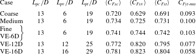
Table 2 includes the body force coefficients obtained from all simulations. The drag coefficients
 $C_{Fx}$
are time-averaged values, while the side force coefficient
 $C_{Fy}$
is the root-mean-square (r.m.s.) value because we have zero mean side force from the simulations. Three drag coefficients are listed in table 2:
 $\langle C_{Fxc}\rangle$
is the mean drag coefficient of the curved part of the cylinder,
 $\langle C_{Fxv}\rangle$
is of the vertical extension part and
 $\langle C_{Fxt}\rangle$
is the drag coefficient of both parts. The drag coefficients are normalized as
 $$\begin{eqnarray}\langle C_{Fxj}\rangle =\frac{\langle F_{xj}\rangle }{0.5\unicode[STIX]{x1D70C}DL_{pj}U_{0}^{2}},\quad j=c,v,t,\end{eqnarray}$$
where the subscript
 $c$
stands for the curved part,
 $v$
for the vertical part and
 $t$
for the curved plus vertical parts. The r.m.s. lift coefficient is normalized in the same way. Notice that the projection length
 $L_{pj}$
(vertical length of the cylinder’s projection into the
 $(y,z)$
-plane) varies for different parts, as listed in table 2.
Calculated force coefficients for the curved part, vertical part and both parts, respectively. The drag coefficients are defined in (2.4). Subscript
 $c$
stands for curved part,
 $v$
for vertical part and
 $t$
for curved plus vertical parts;
 $L_{pj}$
stands for the projection area of the corresponding parts into the
 $(y,z)$
-plane; and
 $C_{Fyt}$
is the r.m.s. value.
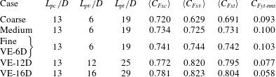
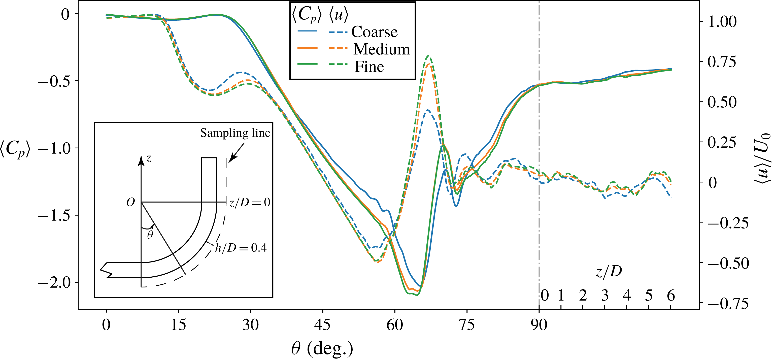
The data in table 2 show converging trends of all force coefficients when the mesh is gradually refined. Besides, in figure 3, we plot the time-averaged streamwise velocity
 $\langle u\rangle /U_{0}$
and the time-averaged pressure coefficient
 $\langle C_{p}\rangle$
(2.5) along a sampling line that follows the cylinder span in the symmetry plane, with
 $h/D=0.4$
apart from the cylinder:
 $$\begin{eqnarray}\langle C_{p}\rangle =\frac{\langle p\rangle -p_{0}}{0.5\unicode[STIX]{x1D70C}U_{0}^{2}},\end{eqnarray}$$
where
 $\langle p\rangle$
is the time-averaged pressure and
 $p_{0}$
is the pressure at the inlet boundary. A sketch depicting the location of the sampling line is included in the lower left corner of figure 3.
Time-averaged pressure coefficient
 $\langle C_{p}\rangle$
and streamwise velocity
 $\langle u\rangle /U_{0}$
plotted along a sampling line. This sampling line is located in the symmetry plane, and
 $h/D=0.4$
apart from the cylinder, indicated by the dashed line in the lower left. Results from all three grid study simulations are collected. The abscissa is divided into two parts: the curved part is measured by angle
 $\unicode[STIX]{x1D703}$
(defined in figure 1), while the straight vertical part is measured by height
 $z/D$
. The length scales in these two parts are not necessarily the same;
 $L_{v}/D=6$
.

Flow around the horizontal extension part has been thoroughly discussed in Jiang et al. (Reference Jiang, Pettersen and Andersson2018a
), so in this paper we focus on flow around the curved and vertical extension parts. Figure 3 shows that the Medium mesh gives close results to those from the Fine mesh, for both the velocity and pressure plots. In most of this figure, we barely see any differences between the Medium and Fine mesh results. The results from the Coarse mesh, however, deviate more in some parts, e.g. the negative peak values at
 $\unicode[STIX]{x1D703}\approx 65^{\circ }$
in both the velocity and pressure plots. Yet results from the coarsest mesh show the same trends as those from the other two meshes. Moreover, the location of the peaks are correctly captured even by the coarsest mesh. The force coefficients in table 2, together with the flow field plots in figure 3, show a clear tendency of grid convergence, and that the Medium mesh gives promisingly close solutions to the Fine mesh.
In order to examine whether the finest mesh gives DNS-quality resolution, we have carefully checked the local grid cell size versus the Kolmogorov length scale
 $\unicode[STIX]{x1D702}$
. The results show that, in the finest grid level, the local grid cell size is always smaller than
 $2\unicode[STIX]{x1D702}$
. This assures that the grid is sufficiently fine to resolve all essential velocity gradients.
A statistical convergence examination is also necessary because the results in §§ 3–5 will be presented based on both instantaneous and time-averaged flow results. The VE-16D case was simulated first for 525 time units (
 $D/U_{0}$
) to ensure that the flow is properly developed, and then continued for another
 $600D/U_{0}$
to collect the statistical data. A careful check has confirmed that the statistical results no longer vary after this long sampling time.
Based on the results presented in this section, we conclude that the Fine mesh (see table 1) is sufficiently good for reliable DNS simulations in the present study. This mesh has six levels of grids, with minimum cell size
 $\unicode[STIX]{x1D6E5}_{c}/D=0.00625$
. It has in total 11 714 grids, each of which has
 $56\times 56\times 56$
uniform Cartesian cells, resulting in a total of
 $2.06\times 10^{9}$
grid cells. For the vertical extension study (see table 1), we will apply the same grid resolution and mesh structure for cases VE-12D and VE-16D. One sees from table 1 that all three vertical extension study cases use more than two billion grid cells; the largest simulation VE-16D uses in total
 $2.91\times 10^{9}$
cells.
All simulations were performed on an SGI ALTIX ICE X SLES – 11sp3 cluster at NTNU. To run case VE-16D, we used 3200 processors (2 GB memory per processor), with the recent improved parallel efficiency of MGLET (Strandenes et al. Reference Strandenes, Pettersen, Andersson and Manhart2017), it took less than 2 s to march the simulation one time step forwards. We have run at least 750 000 time steps in the VE-16D simulation in order to properly collect the statistical data; therefore, this single case cost in total approximately 1.35 million CPU hours.
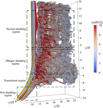
Perspective view of the instantaneous wake obtained from the VE-16D simulation, taken at an arbitrary moment after the flow is fully developed. The wake structures are shown by the isosurface of
 $\unicode[STIX]{x1D706}_{2}=-2$
, and coloured by the instantaneous vorticity magnitude
 $|\unicode[STIX]{x1D714}|D/U_{0}$
. Here we use the transitional regime to indicate the region between the shedding and non-shedding regimes.

3 The vertical length effect at
$Re=3900$

Figure 4 gives an overall impression of the instantaneous wake in the VE-16D simulation by showing a snapshot of the isosurface of
 $\unicode[STIX]{x1D706}_{2}=-2$
(see Jeong & Hussain (Reference Jeong and Hussain1995) for the definition of the vortex identification measure
 $\unicode[STIX]{x1D706}_{2}$
). The snapshot is taken at an arbitrary time, and the isosurface is coloured by the instantaneous vorticity magnitude
 $|\unicode[STIX]{x1D714}|D/U_{0}$
at that moment, just to offer some more information. At
 $Re=3900$
, we still observe similar overall features as in the low-
 $Re$
concave curved cylinder wake (sketched in figure 1). Most parts of the wake turn turbulent, including the oblique shedding regime. The non-shedding regime in the lower part of the wake, nevertheless, remains laminar. Therefore, an intermediate or transitional flow regime exists in the wake, as depicted in figure 4. In this transitional regime, the flow experiences rapid transition from laminar to turbulent flow, creating complex dynamics, which will be discussed in § 4. The focus of the present section will be on the effect of the vertical extension length (
 $L_{v}$
effect).
Snapshots of the instantaneous cross-flow velocity
 $v/U_{0}$
distribution in the symmetry plane (the
 $(x,z)$
-plane at
 $y/D=0$
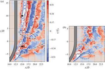
) in (a) the VE-16D simulation and (b) the VE-6D simulation, selected at the same phase of a period instead of at the same time instant. The colour scale is the same for both snapshots. Points A and B in panel (a) are data sampling points. The dashed ellipses indicate interesting phenomena that will be discussed later in the paper.

Snapshot of
 $\unicode[STIX]{x1D706}_{2}=-2$
isosurface in the VE-6D simulation. The isosurface is coloured by the instantaneous vorticity magnitude
 $|\unicode[STIX]{x1D714}|D/U_{0}$
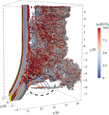
. The region marked by the dashed ellipse gives a 3-D picture of the jagged pattern highlighted in figure 5(b). These vortical structures only appear in the VE-6D simulation.

The
 $L_{v}$
effect is clearly seen when we compare the instantaneous cross-flow velocity (
 $v/U_{0}$
) distributions in the symmetry plane in the VE-16D and VE-6D simulations, as shown in figure 5(a) and 5(b), respectively. Note that we intentionally plot the snapshots at the same phase of the period rather than at the same time instant in order to make the snapshots directly comparable.
The most pronounced difference between the two snapshots in figure 5 is the inclination of velocity strips, i.e. the alternating red (positive
 $v$
) and blue (negative
 $v$
) strips, behind the vertical extensions. These strips represent alternately shedding vortices. One intuitively gets an impression that the upper boundary (
 $z/D=6$
) in figure 5(b) heavily influences the flow below. Moreover, as mentioned in the introduction,
 $L_{v}$
not only influences the flow directly behind the vertical extension, but has also a global influence on the overall wake, i.e. the flow behind the curved part is also affected. This is revealed by carefully observing the flow in the region marked by the dashed ellipse in the lower part of figure 5(b). The jagged pattern in this region corresponds to a series of thin vortex filaments marked by the dashed ellipse in figure 6, where the instantaneous
 $\unicode[STIX]{x1D706}_{2}=-2$
isosurface in the VE-6D simulation is plotted to give a 3-D impression.
The marked vortical structures shown in figure 6 repeatedly emerge in the VE-6D simulation. Therefore, they are not random phenomena. However, they never occur in the VE-16D simulation. Since the comparison between figure 5(a) and 5(b) already shows that the VE-6D results are affected by
 $L_{v}$
, these vortex filament structures in figure 6 will not be discussed further. Nevertheless, they clearly demonstrate the influence of
 $L_{v}$
on the overall wake. Figures 7 and 8 present more quantitative comparisons between simulations with different
 $L_{v}$
.
Contours of
 $\langle \unicode[STIX]{x1D714}_{x}\rangle D/U_{0}=\pm 0.5$
and
 $\pm 1$
plotted in a
 $(y,z)$
-plane located at
 $x/D=14$
. Solid contours indicate positive values, and dashed lines indicate negative values. (a) Comparison between the VE-6D and VE-16D results. (b) Comparison between the VE-12D and VE-16D results. The four major regions with concentrated vorticity are marked as
 $L_{1}$
,
 $L_{2}$
,
 $R_{1}$
and
 $R_{2}$
, respectively in panel (a). All plots are observed from a downstream position.

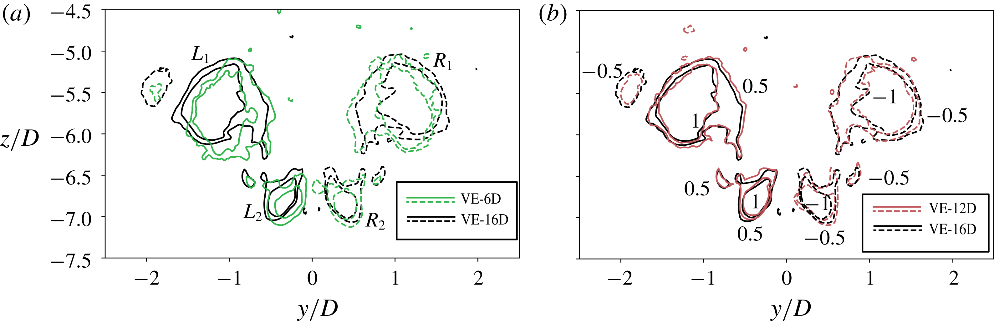
In figure 7, we plot the time-averaged streamwise vorticity
 $\langle \unicode[STIX]{x1D714}_{x}\rangle D/U_{0}$
contours in a (
 $y,z$
)-plane located at
 $x/D=14$
. We note that the results are in the transitional regime, as one can read
 $z/D\subset (-7.5,-4.5)$
from figure 7. Above this regime, we enter the vortex shedding regimes, as indicated in figure 4, where the wake is turbulent and consists of numerous fine and apparently random vortical structures. They will be smoothed out by the time-averaging operation, provided that the statistical sampling time is sufficiently long. However, in the transitional regime, we can still observe concentrated vorticity regions even in the time-averaged results.
The four major regions with concentrated
 $\langle \unicode[STIX]{x1D714}_{x}\rangle$
distributions are marked as
 $L_{1}$
,
 $L_{2}$
,
 $R_{1}$
and
 $R_{2}$
in figure 7(a). The contours show that regions
 $L_{1}$
and
 $L_{2}$
have positive
 $\langle \unicode[STIX]{x1D714}_{x}\rangle$
values, while regions
 $R_{1}$
and
 $R_{2}$
have negative
 $\langle \unicode[STIX]{x1D714}_{x}\rangle$
values. Figure 7(a) indicates two pairs of counter-rotating vortices in the mean flow field, which is an interesting phenomenon that will be discussed in § 4.3. Nevertheless, these concentrated mean vorticity regions reveal the influence from the non-shedding vortex sheets. From figure 7(a) we see that all these regions are captured in both VE-6D and VE-16D simulations. The two sets of contour lines are similarly shaped, except that the results for case VE-6D are slightly shifted downwards (i.e. in
 $-z$
direction) and towards the centre. On the other hand, the comparisons in figure 7(b), i.e. between cases VE-12D and VE-16D, show better agreement. The VE-12 simulation gives very close results to those in VE-16D, with respect to both the shape of the concentrated vorticity regions and their locations. Note that the results from VE-6D and VE-12D are less smooth compared to that from VE-16D, because these two simulations were only meant for
 $L_{v}$
effect investigation, and run for a relatively short time. The results are, nevertheless, already convincing and conclusive.
Time-averaged vertical velocity
 $\langle w\rangle /U_{0}$
plotted along four sampling lines in the symmetry plane, located
 $h/D=0.4$
(black), 0.6 (green), 0.8 (red) and 1.0 (purple) apart from the cylinder, respectively. Results from case VE-16D (solid lines), VE-12D (dashed lines) and VE-6D (dashed-dotted lines) are plotted together for comparison. The curved part is measured by angle
 $\unicode[STIX]{x1D703}$
, while the straight vertical part of the cylinder is measured by
 $z/D$
. A sketch is appended in the upper left corner to depict the sampling line.

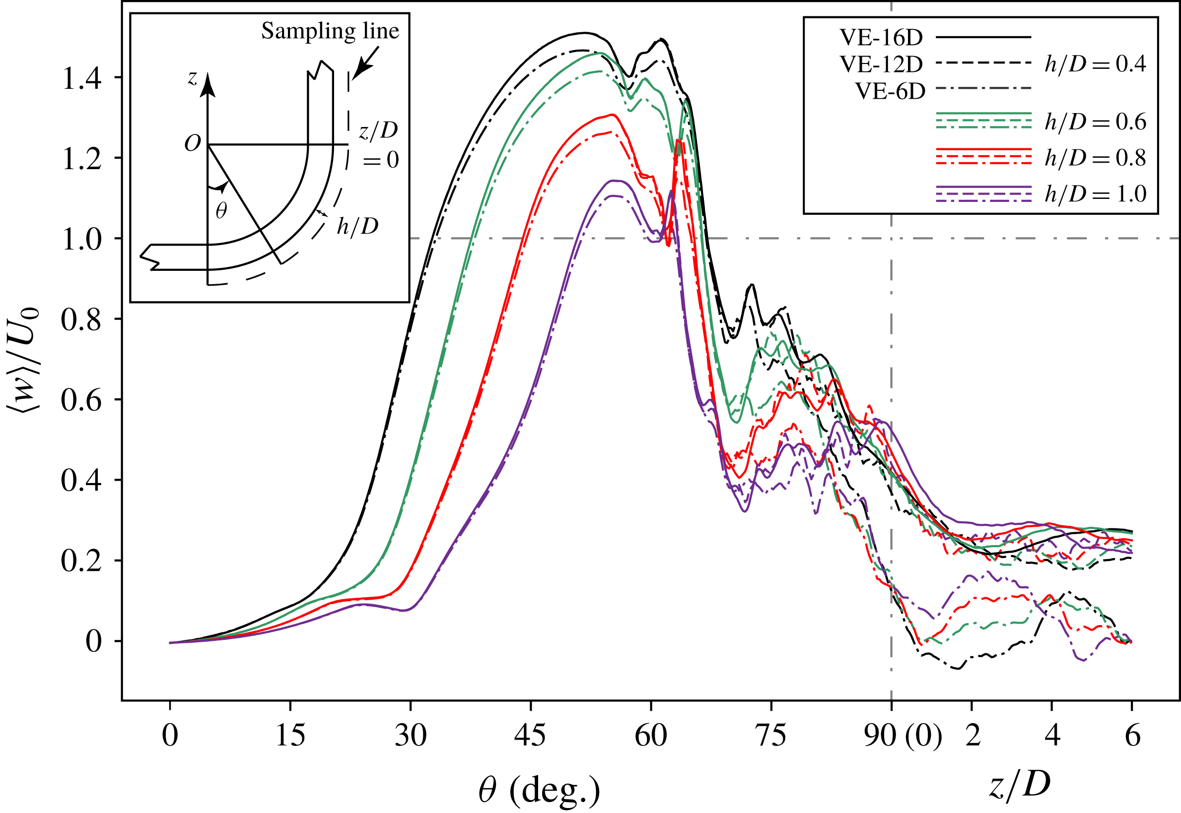
Figure 8 shows the time-averaged velocity component
 $\langle w\rangle /U_{0}$
along four sampling lines in the symmetry plane, i.e. the
 $(x,z)$
-plane at
 $y/D=0$
. The sampling lines follow the span of the cylinder in both the curved and vertical parts, and are located at different distances (
 $h/D=0.4$
, 0.6, 0.8 and 1.0, respectively) behind the cylinder. The results from all three vertical extension study cases are plotted together for easy comparison. The VE-12D and VE-16D results are therefore truncated at
 $z/D=6$
. In figure 8, we first observe unexpectedly high
 $\langle w\rangle$
values in the very near wake. Along the
 $h/D=0.4$
curves,
 $\langle w\rangle$
exceeds the magnitude of the inflow velocity
 $U_{0}$
over a rather wide range
 $\unicode[STIX]{x1D703}\subset (32^{\circ },67^{\circ })$
. Moreover, the maximum
 $\langle w\rangle$
value reaches approximately
 $1.5U_{0}$
. This represents a very strong axial flow in the near wake, which consequently induces the strong oblique shedding. Secondly, we can hardly distinguish between the solid lines (VE-16D results) and dashed lines (VE-12D results) in figure 8 when
 $\unicode[STIX]{x1D703}\lessapprox 75^{\circ }$
. Even beyond
 $\unicode[STIX]{x1D703}\approx 75^{\circ }$
, the differences between the lines are small. These comparisons show that the VE-12D and VE-16D simulations give very close results. The VE-6D results (dashed-dotted lines in figure 8) deviate more from the other two simulations, especially when
 $\unicode[STIX]{x1D703}\gtrapprox 80^{\circ }$
. Moreover, we notice that the results of case VE-6D deviate more from those of VE-12D and VE-16D in the vertical extension part. This is another strong indication that the free-slip wall boundary condition at the top has very strong influence on the results in the VE-6D case.
In summary, both the comparison between the instantaneous flow fields (figure 5
a and 5
b) and that between the time-averaged flow fields (figures 7 and 8) show
 $L_{v}$
effects in the concave curved cylinder wake at
 $Re=3900$
. The VE-6D results deviate somewhat from the VE-16D results. Therefore, an
 $L_{v}/D=6$
vertical extension is not long enough and not a satisfactory choice for the quarter-ring concave curved cylinder configuration. The results of the VE-12D simulation are rather close to those of the VE-16D simulation, showing a good convergence trend. From the discussions in this section, we are convinced that
 $L_{v}=16D$
will be sufficient for this particular flow simulation. The following discussions are therefore all based on results from the VE-16D simulation.
4 The wake dynamics
4.1 Flow regimes and vortex dislocations
An eye-catching feature of this wake flow is the distinct frequencies in different flow regimes, accompanied by massive vortex dislocations. This is easily observed in figure 5(a), where distinct flow structures are observed in different coexisting flow regimes. Slightly inclined alternating red (positive
 $v$
) and blue (negative
 $v$
) strips manifest themselves in the upper part (
 $z/D>2$
) of the snapshot, revealing regular von Kármán vortex shedding, with a modest oblique shedding angle. In the lower part of the snapshot in figure 5(a), however, the flow is more complex. In a certain area around
 $z/D\approx 0$
, the alternating velocity strips are distinctly wider and more tilted than in the upper part, indicating more oblique shedding with a longer period.
(a) The power spectral density of all three velocity components at sampling point A, indicated in figure 5(a), whose coordinates are
 $(x/D,y/D,z/D)=(15,0,10)$
. (b) The same as in panel (a) but for sampling point B with coordinates
 $(15,0,-2)$
.

The power spectral density of
 $v/U_{0}$
plotted over a vertical sampling line in the symmetry plane, located at
 $x/D=15.0$
. The
 $z/D$
value varies from
 $-6.0$
to 16.0.

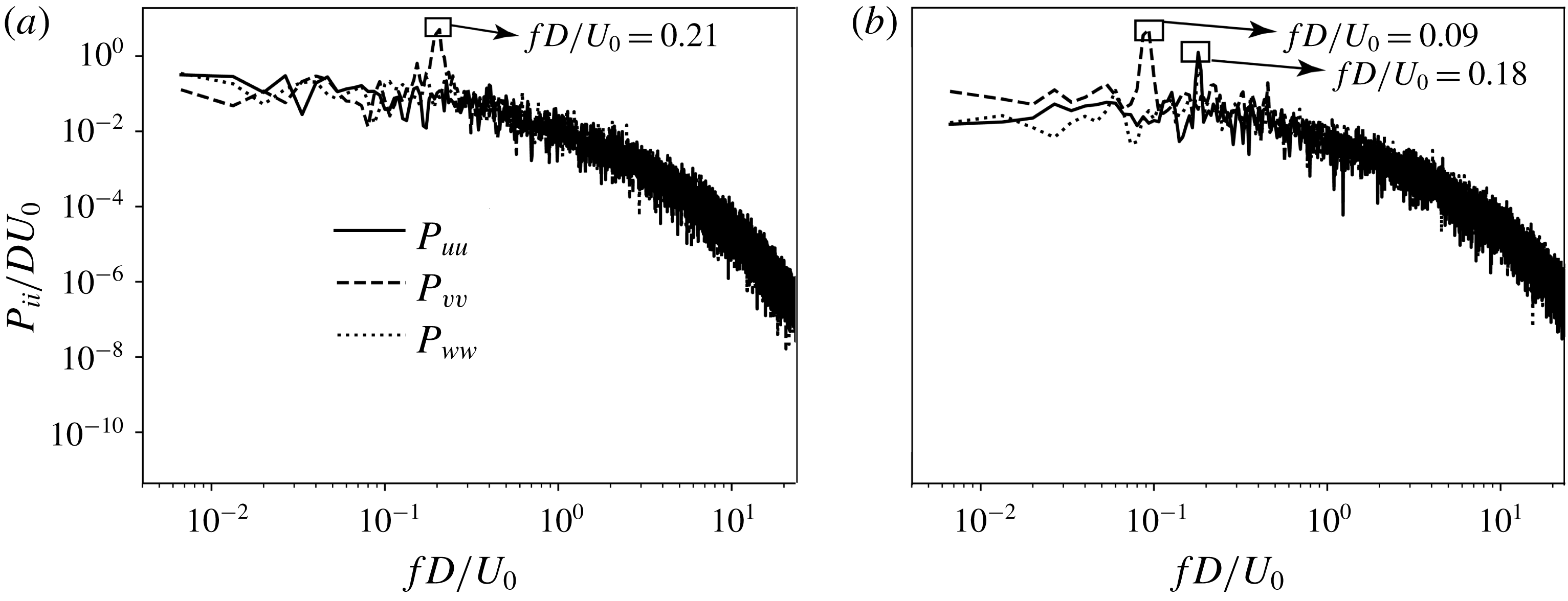
Figures 9(a) and 9(b) show the power spectral density of the three velocity components at two selected sampling points in the symmetry plane, i.e. points A and B, respectively. The locations of these two sampling points are marked as large dots in figure 5(a), where we see that they are positioned in different flow regimes. Velocity signals are collected every second time step, giving a sampling period of
 $0.003D/U_{0}$
. In total 131 072 sampling values were collected to ensure long enough sampling time (
 ${\approx}393.2D/U_{0}$
). Welch’s method (Welch Reference Welch1967) was used to calculate the spectral density in figure 9(a,b). A Hanning window was employed with window width of 65 536 to reduce background artifacts in amplitudes. Figure 9(a) clearly shows a dominating frequency of
 $fD/U_{0}=0.21$
at point A, which is close to the parallel shedding frequency for a straight circular cylinder at the same
 $Re=3900$
(see e.g. Parnaudeau et al.
Reference Parnaudeau, Carlier, Heitz and Lamballais2008). The dominating frequency
 $fD/U_{0}=0.09$
read from figure 9(b) is, on the other hand, distinctly lower than the parallel shedding frequency, which is in qualitative agreement with the observations in figure 5(a) that the vortex shedding in the lower wake has longer period. We note that in figure 9(b), the dominating frequency in
 $P_{uu}$
and
 $P_{ww}$
(
 $fD/U_{0}=0.18$
) is twice that in
 $P_{vv}$
. This is because the sampling point is located in the symmetry plane.
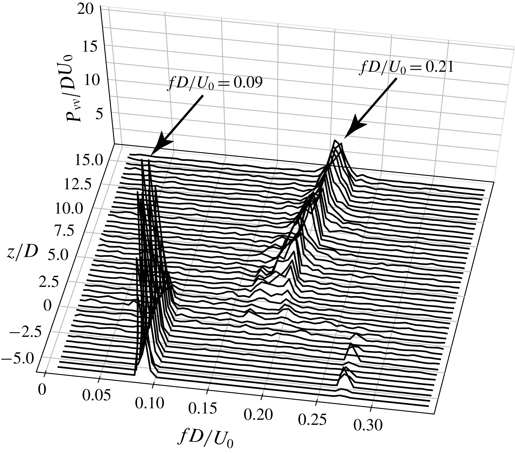
Figure 10 gives a more comprehensive picture of the frequency differences in the wake, by plotting the power spectral density of
 $v/U_{0}$
over a vertical sampling line in the symmetry plane (the
 $(x,z)$
-plane at
 $y/D=0$
) located at
 $x/D=15.0$
. Notice that we do not use a log scale in figure 10, and only show the spectra in the range
 $fD/U_{0}\leqslant 0.35$
, in order to focus on the interesting frequencies. In figure 10, we observe that the dominating frequency
 $fD/U_{0}=0.09$
in the lower wake (
 $z/D\lessapprox 2.5$
) is constant, while the dominating frequency in the upper wake experiences a mild gradual increase from
 $fD/U_{0}\approx 0.19$
to 0.21. A similar scenario was reported at
 $Re=400$
and 500 for the same geometrical configuration in Jiang et al. (Reference Jiang, Pettersen, Andersson, Kim and Kim2018b
).
An abrupt frequency change shows up at
 $z/D\approx 2.5$
(see figure 10) along the sampling line (at
 $x/D=15$
). This is consistent with the snapshot in figure 5(a), where vortex dislocations are observed in the area indicated by a dashed ellipse. The mechanism behind vortex dislocations is the phase difference between neighbouring vortices (Williamson Reference Williamson1996). In the wake behind various cylinder configurations, the phase differences mostly originate either from spanwise non-uniformities (see e.g. Tian et al.
Reference Tian, Jiang, Pettersen and Andersson2017) or from end effects (see e.g. Williamson Reference Williamson1989). In our case, we clearly observe from figure 5(a) that dislocations are closely related to the strong oblique shedding in the lower wake. This has been accepted to be a result of the strong axial flow in the concave curved cylinder wake (see e.g. Miliou et al.
Reference Miliou, de Vecchi, Sherwin and Graham2007; Jiang et al.
Reference Jiang, Pettersen, Andersson, Kim and Kim2018b
; Shang et al.
Reference Shang, Stone and Smits2018). The strong axial flow, as a representative characteristic of this wake, essentially originates from the curved span of the cylinder (Jiang et al.
Reference Jiang, Pettersen, Andersson, Kim and Kim2018b
). Therefore, although the dislocations in the present case only show up behind the vertical extension (
 $z/D>0$
) whose span is uniform, their origin is still the spanwise non-uniformity of the curved cylinder. Nevertheless, due to the relatively large frequency difference in the present case, the dislocations become severe in this area. In figure 5(a), we also observe that the dislocations happen at different
 $z/D$
positions as
 $x/D$
varies. The animation in supplementary movie 1 (available at https://doi.org/10.1017/jfm.2019.648) presents a sequence of similar snapshots as figure 5(a), from which the dynamics can be more clearly understood.
4.2 New characteristics and perspectives of the axial flow
Strong axial flow in the concave curved cylinder wake at low
 $Re$
has been reported and explained in previous studies (see Miliou et al.
Reference Miliou, de Vecchi, Sherwin and Graham2007; Jiang et al.
Reference Jiang, Pettersen, Andersson, Kim and Kim2018b
; Shang et al.
Reference Shang, Stone and Smits2018), and considered as the main reason why oblique shedding and various flow regimes coexist in the flow. However, by plotting the time-averaged axial velocity
 $\langle u_{ax}\rangle /U_{0}$
along several lines in the near wake (figure 11), we observe some distinct and noteworthy features compared to our previous knowledge at lower
 $Re$
. Earlier in figure 8, we already observed a high vertical velocity
 $\langle w\rangle$
in the near wake. Yet, since the cylinder span is curved, the streamwise velocity
 $\langle u\rangle$
also contributes to the actual axial velocity. In figure 11
 $\langle u_{ax}\rangle$
is therefore calculated as
 $u_{ax}=u\cos \unicode[STIX]{x1D703}+w\sin \unicode[STIX]{x1D703}$
.
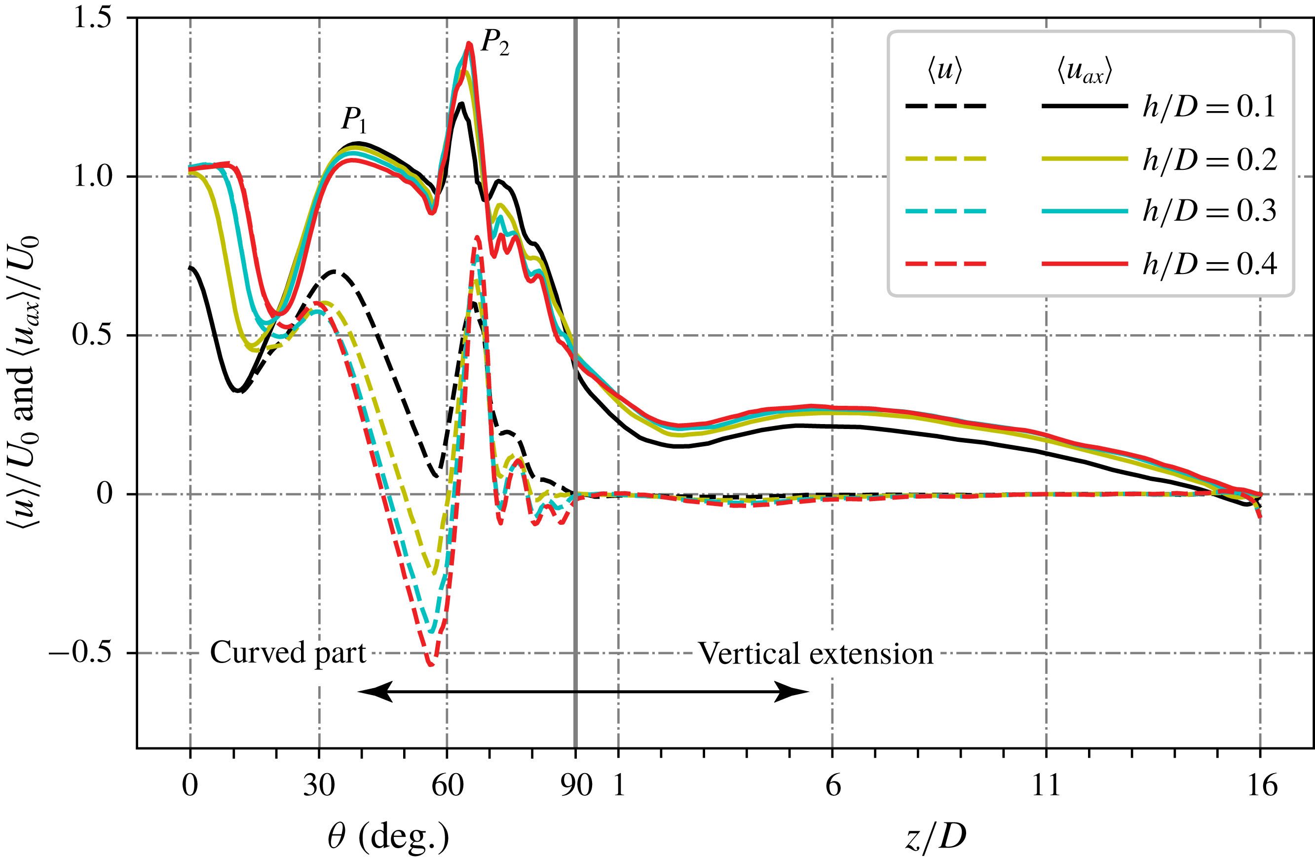
Time-averaged axial velocity
 $\langle u_{ax}\rangle /U_{0}$
(solid lines) and streamwise velocity
 $\langle u\rangle /U_{0}$
(dashed lines) plotted over four sampling lines in the symmetry plane along the cylinder span. Results from simulation VE-16D. The sampling lines are arranged in a similar way as sketched in figure 8, where
 $h/D$
denotes the distance from the cylinder surface.

We note two distinct new phenomena in figure 11. First, two peaks (
 $P_{1}$
and
 $P_{2}$
) can be spotted in the
 $\langle u_{ax}\rangle$
distributions, while only one peak (corresponding to
 $P_{1}$
) was reported in the lower-
 $Re$
flows (see figures 5 and 7 in Jiang et al. (Reference Jiang, Pettersen, Andersson, Kim and Kim2018b
)). The physics behind peak
 $P_{1}$
has been well understood from earlier studies (e.g. Jiang et al.
Reference Jiang, Pettersen, Andersson, Kim and Kim2018b
) and attributed to the generation and development of a vortex sheet pair. However, the physics behind the newly observed peak
 $P_{2}$
is unclear and will be investigated in this subsection. The previously known peak
 $P_{1}$
has
 $\langle u_{ax}\rangle$
values comparable in magnitude to the incoming velocity
 $U_{0}$
, both at
 $Re=3900$
and at lower
 $Re$
. These are already high axial velocity values. However, the
 $\langle u_{ax}\rangle$
values at
 $P_{2}$
, as read from figure 11, are even higher, and reach up to
 $1.4U_{0}$
.
Secondly, we observe high streamwise velocity
 $\langle u\rangle$
values at approximately the same spanwise location as
 $P_{2}$
for
 $\langle u_{ax}\rangle$
, i.e. at
 $\unicode[STIX]{x1D703}\approx 65^{\circ }$
. If we recall the
 $\langle w\rangle$
results in figure 8, we also notice a local peak in the
 $\langle w\rangle$
distributions at roughly the same location. Neither of them were observed in the lower-
 $Re$
flows of the same configuration (e.g. Jiang et al.
Reference Jiang, Pettersen, Andersson, Kim and Kim2018b
). The second peak in figure 8 is more easily overlooked due to the continuously high
 $\langle w\rangle$
values (larger than
 $U_{0}$
) over a wider span compared to
 $\langle u\rangle$
and
 $\langle u_{ax}\rangle$
shown in figure 11.
The first peak
 $P_{1}$
is in the non-shedding regime, where the physical meaning behind the variations in
 $\langle w\rangle$
and
 $\langle u\rangle$
can be explained by the vortex sheet production and cylinder shelter effect, respectively, as addressed in Jiang et al. (Reference Jiang, Pettersen, Andersson, Kim and Kim2018b
) for lower-
 $Re$
flows. It is therefore reasonable to further explain
 $P_{1}$
in
 $\langle u_{ax}\rangle$
as a joint effect of
 $\langle w\rangle$
and
 $\langle u\rangle$
. However, this does not necessarily mean that
 $\langle u_{ax}\rangle$
is a result of
 $\langle u\rangle$
and
 $\langle w\rangle$
; they are just different measures of the near-wake velocity in different coordinate systems. In fact, it becomes confusing if we try to explain
 $P_{2}$
in
 $\langle u_{ax}\rangle$
in the same way as we did for
 $P_{1}$
. Although we observe separated peaks for
 $\langle u\rangle$
(in figure 11) and
 $\langle w\rangle$
(in figure 8) at
 $\unicode[STIX]{x1D703}\approx 65^{\circ }$
, they are somewhat opposed to the general understanding of the wake flow, as explained in the following.
The production process of the vortex sheets described in Jiang et al. (Reference Jiang, Pettersen, Andersson, Kim and Kim2018b
) ends as the vortex sheets start to shed. This is indicated by the small drop in
 $\langle w\rangle$
between the two peaks (see figure 8). An intuitive scenario is like what we observed in the low-
 $Re$
wakes, i.e. this drop continues for all three velocity components
 $\langle u\rangle$
,
 $\langle w\rangle$
and
 $\langle u_{ax}\rangle$
(see figure 12 in Jiang et al. (Reference Jiang, Pettersen, Andersson, Kim and Kim2018b
)). But at
 $Re=3900$
, all three velocities increase again. The peak of
 $\langle u\rangle$
at
 $\unicode[STIX]{x1D703}\approx 65^{\circ }$
is especially confusing. We note that
 $\unicode[STIX]{x1D703}\approx 65^{\circ }$
(which corresponds to
 $z/D\approx -6$
in the Cartesian coordinate system) is already in the shedding regime, because we have detected a prominent dominating frequency
 $fD/U_{0}=0.09$
at
 $z/D=-6$
(see figure 10). Consequently, we would expect a recirculation bubble in the time-averaged flow field. Considering that our sampling locations are all very close to the cylinder (
 $h/D\leqslant 0.4$
), and a conventional recirculation area behind a circular cylinder at
 $Re=3900$
can reach approximately
 $1.5D$
behind the cylinder (Parnaudeau et al.
Reference Parnaudeau, Carlier, Heitz and Lamballais2008), we should have expected negative
 $\langle u\rangle$
here instead of a local peak value even higher than
 $0.5U_{0}$
. This peak value in
 $\langle u\rangle$
is therefore rather abnormal. In other words, we need to seek the physics behind
 $P_{2}$
in the
 $\langle u_{ax}\rangle$
distribution (figure 11) from another point of view.
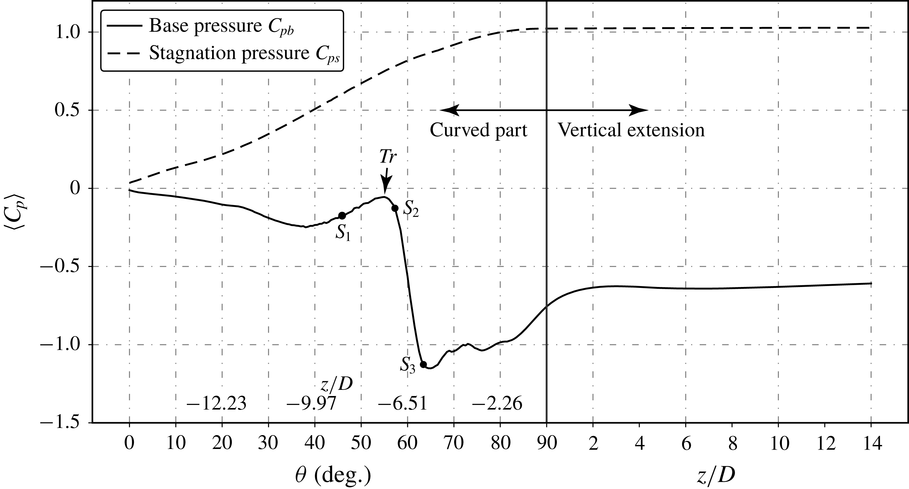
Time-averaged base pressure
 $C_{pb}$
and stagnation pressure
 $C_{ps}$
distributions along the span of the cylinder. Pressure values are interpolated
 $h=0.015D$
apart from the base (stagnation) line. The spanwise location is indicated in different scales for the curved and vertical extension parts, as in previous figures. But
 $z/D$
values are additionally marked for the curved part in this figure. They are calculated based on the base pressure line, i.e. with radius
 $13.015D$
. This is to give a quick reference to the positions in the Cartesian coordinate system.

Figure 12 shows the time-averaged base pressure
 $C_{pb}$
and stagnation pressure
 $C_{ps}$
distributions along the cylinder span (except for the horizontal part). It is worth mentioning that, with IBM, smooth surface pressure distributions are difficult. This is a known shortcoming of IBM due to the way a curved surface is interpreted. The ‘surface pressure coefficients’ plotted in figure 12 are interpolated values at two lines
 $0.015D$
away from the base and stagnation lines, respectively. The distance
 $h=0.015D$
is chosen because it is slightly larger than the smallest cell’s diagonal (
 $\sqrt{3}\unicode[STIX]{x1D6E5}_{c}<h=0.015D<1.5\sqrt{3}\unicode[STIX]{x1D6E5}_{c}$
, where
 $\unicode[STIX]{x1D6E5}_{c}=0.00625D$
), such that we safely avoid wiggles possibly caused by cells directly cut by the solid surface, and still stay as close as possible to the surface.
In figure 12, we observe that the base pressure experiences a sharp drop in the range from
 $\unicode[STIX]{x1D703}\approx 55^{\circ }$
to
 $\unicode[STIX]{x1D703}\approx 65^{\circ }$
. At
 $\unicode[STIX]{x1D703}<55^{\circ }$
we are in the non-shedding regime where the wake is dominated by a counter-rotating vortex sheet pair. In a circular cylinder wake, it is well known that the base pressure reaches a minimum at the Reynolds number when the wake transits from steady to unsteady (see e.g. figure 1 in Roshko (Reference Roshko1993) and figure 4.12 in Zdravkovich (Reference Zdravkovich1997)). After the wake becomes unsteady, the base pressure increases with
 $Re$
in a certain range. A similar tendency is observed in figure 12 around point
 $Tr$
indicated therein. We can therefore reasonably assume that the vortex sheet pair transits from a steady non-shedding regime to an unsteady shedding regime at
 $\unicode[STIX]{x1D703}\approx 55^{\circ }$
.
It is worth mentioning that we can also observe a mild favourable pressure gradient at
 $\unicode[STIX]{x1D703}<40^{\circ }$
in figure 12. However, this favourable pressure gradient does not lead to acceleration of the flow for two reasons. First, in the near wake when viscous effects are strong, the Bernoulli equation is not necessarily valid. Second, even if the Bernoulli equation is valid, this favourable pressure gradient is small compared to that around
 $\unicode[STIX]{x1D703}\approx 60^{\circ }$
. Therefore, it could not lead to a sufficient velocity increase to compensate for the velocity reduction induced by the shelter effect of the cylinder, as explained in Jiang et al. (Reference Jiang, Pettersen, Andersson, Kim and Kim2018b
).
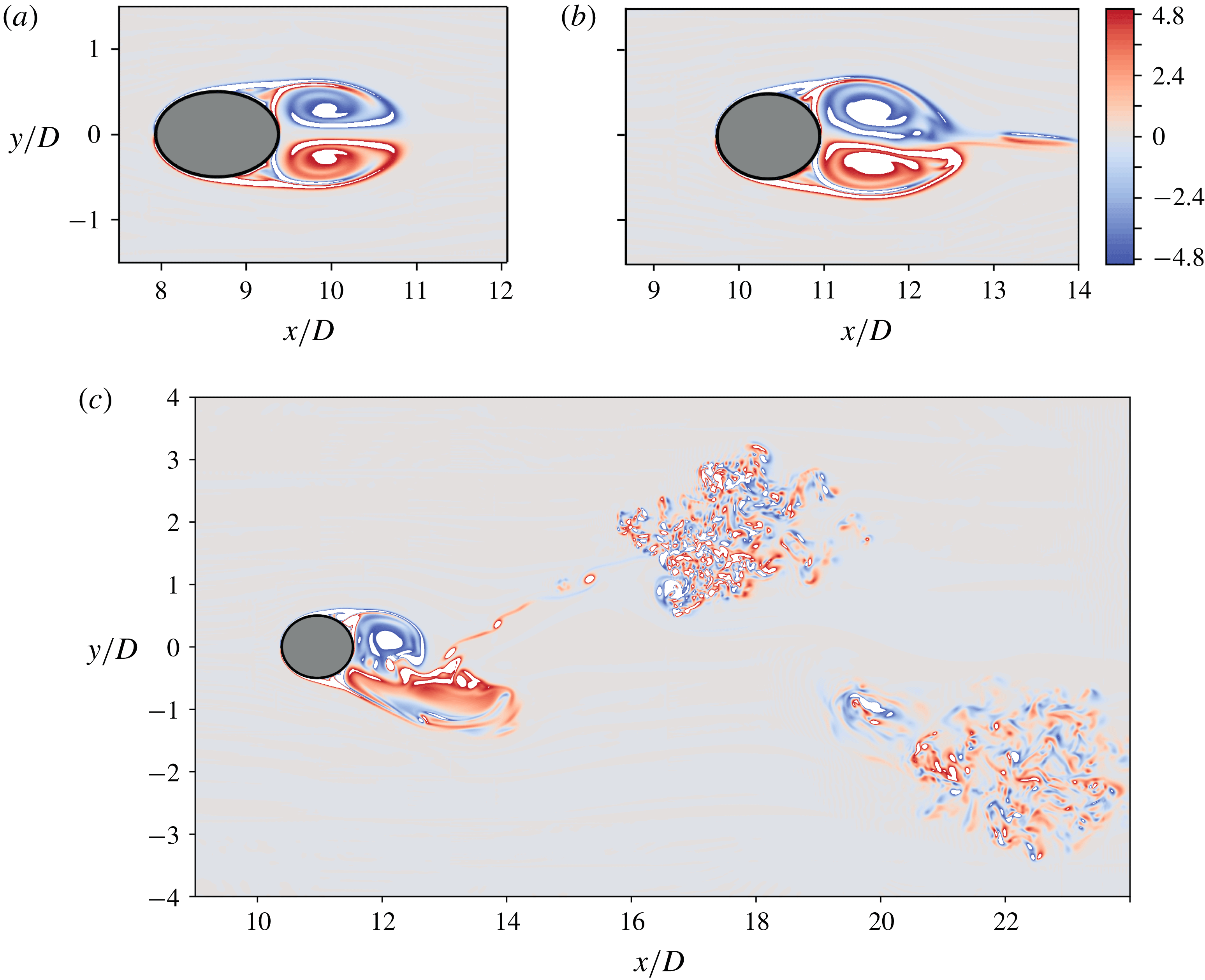
Instantaneous
 $\unicode[STIX]{x1D714}_{z}$
snapshots plotted in three horizontal planes at
 $z/D=-9.0$
(a),
 $-7.0$
(b) and
 $-6.0$
(c). The locations of the three horizontal planes are marked as
 $S_{1}$
,
 $S_{2}$
and
 $S_{3}$
on the base pressure distribution in figure 12. Panels (a–c) use the same colour scale, as shown to the upper right. Time is
 $t=1125D/U_{0}$
.

More detailed flow visualizations are presented in figure 13(a–c), where the instantaneous vertical vorticity component
 $\unicode[STIX]{x1D714}_{z}D/U_{0}$
is plotted in three selected horizontal planes (referred to as
 $z$
-cuts in this paper) at
 $z/D=-9.0$
,
 $-7.0$
and
 $-6.0$
, respectively. The corresponding locations of these three horizontal planes are marked with black dots in figure 12, and respectively denoted as
 $S_{1}$
,
 $S_{2}$
and
 $S_{3}$
. The plane in figure 13(a) is in the non-shedding regime. Here, we clearly see that the wake is laminar and symmetric behind the elliptical cross-section. Figure 13(b) is the plane at
 $z/D=-7.0$
, corresponding to
 $S_{2}$
(
 $\unicode[STIX]{x1D703}=57.5^{\circ }$
) in figure 12, just after the transition point
 $Tr$
. From figure 13(b), we observe that the wake just starts to become unsteady, the two vortex sheets tend to oscillate in the
 $y$
direction, but shedding barely happens. Further checks reveal that in the plane
 $z/D=-7.0$
, only a small part of the vortex tail is shed into the wake, while the two main vortices with concentrated
 $\unicode[STIX]{x1D714}_{z}$
, representing the vortex sheet pair in the plane, remain attached to the cylinder. An animation of the wake dynamics in the
 $z/D=-7.0$
plane is provided as supplementary movie 2, which gives a better impression of the dynamics. By comparing figure 13(a) and 13(b), our assumption that point
 $Tr$
(in figure 12) is where the vortex sheet pair transits from steady to unsteady is confirmed.
Figure 13(c) shows
 $\unicode[STIX]{x1D714}_{z}$
contours in the
 $z/D=-6.0$
plane, corresponding to
 $\unicode[STIX]{x1D703}=62.5^{\circ }$
(and point
 $S_{3}$
) in figure 12. This is close to where the
 $C_{pb}$
curve reaches its minimum and suction is maximum. We note that figure 13(c) shows a similar pattern as the primary instability in a straight cylinder laminar wake. It is therefore surprising to see very clear turbulence in the downstream region. An explanation of this unexpected scenario will be presented in § 4.3. One can also get an intuitive impression of the dynamics in the
 $z/D=-6.0$
plane via the animation in supplementary movie 3. Moreover, we have noticed earlier from figure 5(a) that the flow is less recognizable in the area around
 $z/D=-6$
, namely the transitional regime. All these results strongly suggest that the transitional regime is special; the flow dynamics therein is very complicated and perhaps detailed attention has not been paid to this in earlier studies. This will be discussed in more detail in § 4.3.
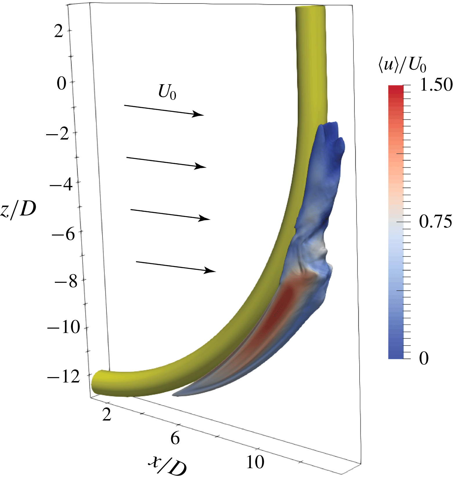
In figure 14 we outline a 3-D picture of the high-axial-flow region by plotting the isosurface of
 $\langle w\rangle /U_{0}=0.6$
coloured by
 $\langle u\rangle /U_{0}$
, from which we see that this region is confined in the very near wake.
Isosurface of
 $\langle w\rangle /U_{0}=0.6$
coloured by
 $\langle u\rangle /U_{0}$
, to give a 3-D perspective picture of the high axial flow we discuss.

From the results and discussions in this subsection, we learned that the strong favourable base pressure gradient along the span of the curved cylinder, in the range from
 $\unicode[STIX]{x1D703}\approx 55^{\circ }$
to
 $\unicode[STIX]{x1D703}\approx 65^{\circ }$
, provides a reasonable explanation for why the second peak
 $P_{2}$
shows up in the axial velocity distribution in figure 11. This second peak in the axial velocity distribution is a new phenomenon that has not been reported and investigated before.
4.3 One frequency – two mechanisms
As discussed in § 4.1, vortex dislocations are prominent in the present wake and can easily be identified as the ‘border’ between the parallel shedding and the oblique shedding regimes. In figure 5(a), we notice that this ‘border’ is not parallel to the
 $x$
direction, but is slightly tilted, due to the strong axial flow in the near wake. At
 $x/D=15.0$
, vortex dislocations occur at around
 $z/D=2.5$
. Below this
 $z$
position, the wake in the shedding regime is dominated by a single uniform low frequency
 $fD/U_{0}=0.09$
. This is clearly illustrated in figures 9(b) and 10. In the low-
 $Re$
concave curved cylinder wake studied earlier, this frequency is related only to the oblique shedding (see figure 10 in Jiang et al. (Reference Jiang, Pettersen, Andersson, Kim and Kim2018b
)). However, at
 $Re=3900$
in the present study, we observe that the wake between the parallel shedding and non-shedding regimes is more complicated. In figure 13(c), we also observed an atypical shedding pattern. It is therefore important to explore the wake dynamics in this area in more detail.
Four
 $\unicode[STIX]{x1D714}_{z}D/U_{0}$
snapshots plotted in a horizontal plane at
 $z/D=-2.0$
over one time period
 $T$
(determined by the corresponding frequency
 $fD/U_{0}=0.09$
). This plane is in the oblique shedding regime. In this figure,
 $t_{0}\approx 1128D/U_{0}$
. All snapshots use the same colour scale.

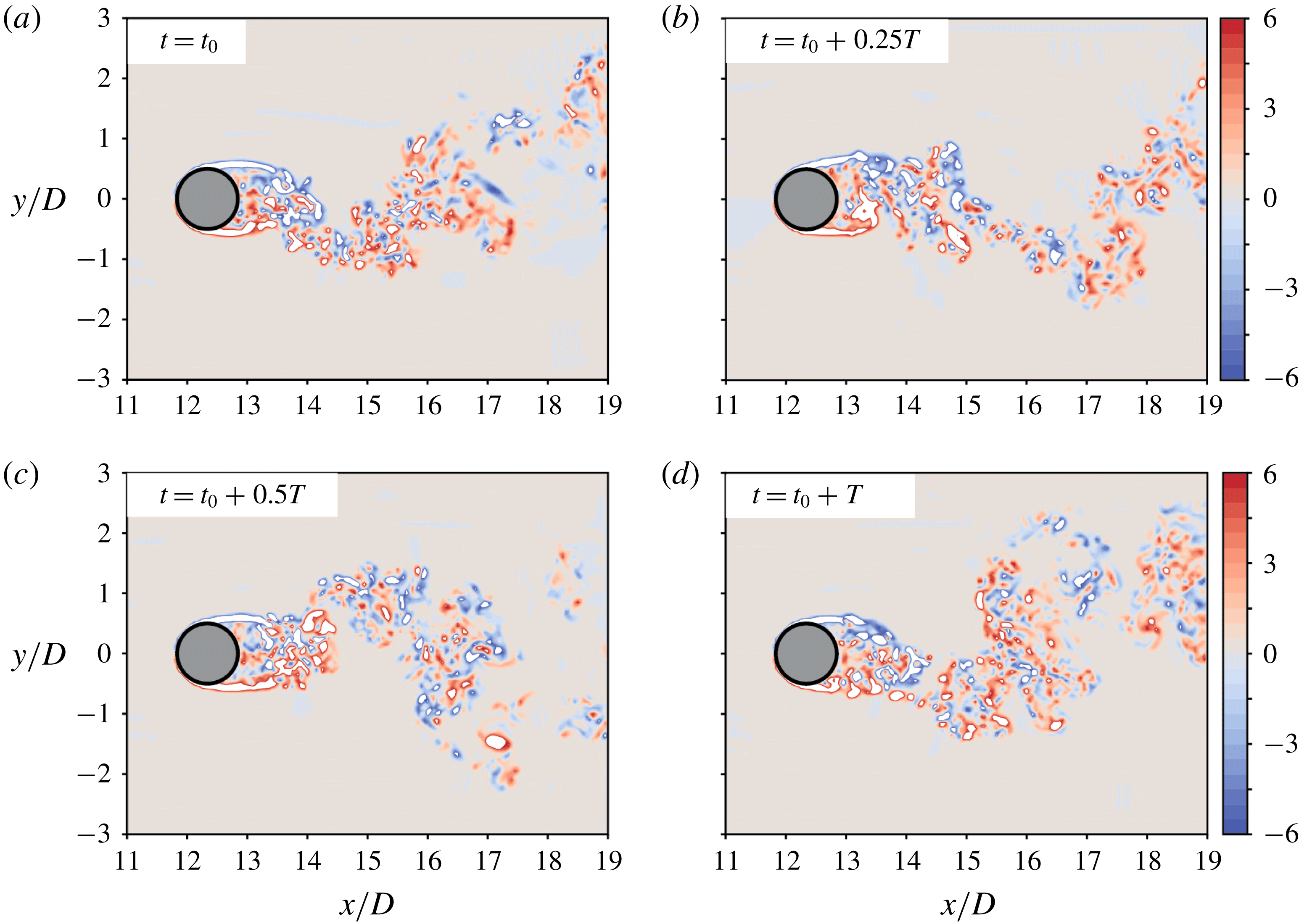
Figure 15 shows four snapshots of the
 $\unicode[STIX]{x1D714}_{z}$
distribution in the
 $z/D=-2.0$
plane over one period of time
 $T$
, which is determined by the dominating frequency
 $fD/U_{0}=0.09$
. With reference to figure 5(a), we know that the horizontal plane at
 $z/D=-2.0$
is in the oblique shedding regime. Despite the relatively long period, the snapshots in figure 15 outline a turbulent von Kármán type shedding, but not similar to that in the circular cylinder wake at the same
 $Re=3900$
(see e.g. Parnaudeau et al.
Reference Parnaudeau, Carlier, Heitz and Lamballais2008). This is understandable because we are not in a parallel shedding regime. However, the relatively short shear layers and the turbulence close to the cylinder in figure 15 are apparently unexpected, because they are typical characteristics of a circular cylinder wake in the upper subcritical state, or more precisely in TrSL3 (
 $Re>20\,000$
) as referred to in Zdravkovich (Reference Zdravkovich1997). Reynolds number
 $Re=3900$
is otherwise considered to be in the TrSL2 state. One may claim that the borders between these two states are not strict, but considering that we are in an oblique shedding regime and the cross-section of the cylinder at
 $z/D=-2.0$
is still slightly elliptic (i.e. more slender than a circular cylinder), we should clearly expect the wake state to be closer to the lower boundary of the subcritical state TrSL1 rather than to the upper boundary towards TrSL3. This assumption is also supported by the fact that oblique shedding postpones the onset of the shear layer instability in a cylinder wake (Prasad & Williamson Reference Prasad and Williamson1997). Anyway, we could not find the shedding pattern in figure 15 to resemble typical TrSL1 flow visualizations (see e.g. figure 40 in Gerrard (Reference Gerrard1978)), meaning that the oblique shedding here is affected by other physics and thus becomes atypical. At lower
 $z$
positions, the shedding in a
 $z$
-cut (an
 $(x,y)$
-plane) becomes even more different from a typical von Kármán shedding pattern (as already observed in figure 13(c) at
 $z/D=-6$
). This again suggests that the flow in this area is probably dominated by different dynamics, for which we need to seek explanations from the non-shedding regime.
The main wake structures in the laminar non-shedding regime are the rolled-up vortex sheets on the two sides of the curved cylinder. Similar vortex sheet structures are reported in various wakes, e.g. sharp-nosed cylinders at high incidence (Thomson & Morrison Reference Thomson and Morrison1971), and prolate spheroids at high incidence (Jiang et al.
Reference Jiang, Gallardo, Andersson and Zhang2015, Reference Jiang, Gallardo, Andersson and Okulov2016), etc. A common feature of these wakes is the continuously inclined or curved separation line. When the vortex sheets separate from the object and shed into the wake, they naturally evolve into a counter-rotating helical vortex pair. More interestingly, this kind of helical vortex pair is mostly asymmetric and non-periodic. Zdravkovich (Reference Zdravkovich1997, p. 983) summarized, based on earlier research, that there may appear several such asymmetric helical vortex pairs along the span of an inclined cylinder. Each pair stays almost at a fixed position to form an alternating vortex street that can be observed in a cross-sectional plane. The helical vortex pair in an inclined prolate spheroid wake is also asymmetric: when the symmetry of the pair is lost, the wake randomly deflects to one side or the other and never turns back again, resulting in a substantial time-averaged side force acting on the spheroid, as comprehensively reviewed in Andersson, Jiang & Okulov (Reference Andersson, Jiang, Okulov and Gelfgat2019). In both situations, the asymmetric helical vortex pairs are mostly in the streamwise direction rather than in the spanwise direction. This leads us to explore the flow in vertical planes normal to the inflow direction, namely (
 $y,z$
)-planes (
 $x$
-cuts).
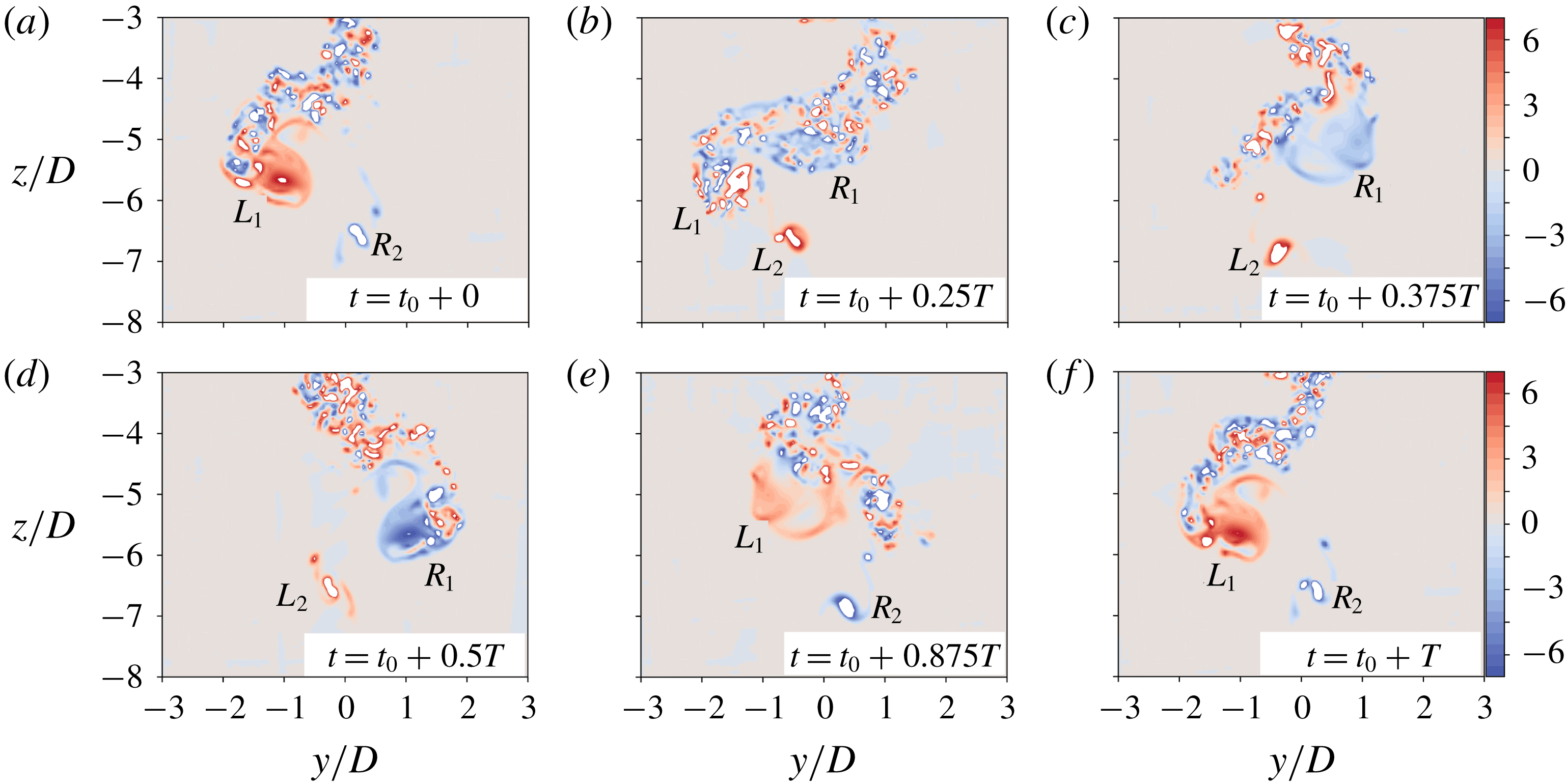
The time-averaged streamwise vorticity distribution in a (
 $y,z$
)-plane located at
 $x/D=14.0$
was presented earlier in figure 7 but not discussed in detail. In figure 16, we show six snapshots of the instantaneous streamwise vorticity
 $\unicode[STIX]{x1D714}_{x}$
plotted in the same
 $(y,z)$
-plane to show the wake dynamics over one time period
 $T$
. Notice that
 $T$
is determined by the same frequency
 $fD/U_{0}=0.09$
as in figure 15.
Six
 $\unicode[STIX]{x1D714}_{x}D/U_{0}$
snapshots plotted in a vertical (
 $y,z$
)-plane positioned at
 $x/D=14.0$
over one time period
 $T$
(determined by the corresponding frequency
 $fD/U_{0}=0.09$
). All snapshots are observed from a downstream position, and use the same colour scale. In this figure
 $t_{0}\approx 1125D/U_{0}$
.

The snapshot in figure 16(a) is arbitrarily chosen at
 $t=t_{0}\approx 1125D/U_{0}$
, from which we immediately identify the asymmetric counter-rotating helical vortex pair as marked by
 $L_{1}$
and
 $R_{2}$
, respectively. Vortex
 $L_{1}$
has positive
 $\unicode[STIX]{x1D714}_{x}$
and rotates anticlockwise (figure 16 is observed from a downstream position), while vortex
 $R_{2}$
has negative
 $\unicode[STIX]{x1D714}_{x}$
and rotates clockwise. Vortex
 $L_{1}$
is larger in size and is located at a higher
 $z$
position;
 $R_{2}$
is located at a lower
 $z$
position, and is smaller in size, but
 $\unicode[STIX]{x1D714}_{x}$
is very concentrated. In figure 16(b), i.e. after
 $0.25T$
,
 $R_{2}$
disappears and
 $L_{1}$
is heavily disintegrated. Meanwhile, a concentrated negative
 $\unicode[STIX]{x1D714}_{x}$
region (
 $R_{1}$
) emerges. It is interesting to notice the striking similarities between figure 16(b) in this paper and figure 4 in Jiang et al. (Reference Jiang, Gallardo, Andersson and Zhang2015); the latter is in the wake behind an inclined prolate spheroid. This might indicate that we observe the same type of vortical structures. However, we must notice that figure 16(b) is an instantaneous snapshot, while figure 4 in Jiang et al. (Reference Jiang, Gallardo, Andersson and Zhang2015) is a time-averaged plot. This major difference tells us that the vortices in these two wakes evolve differently with time.
In figure 16(c), at
 $t=t_{0}+0.375T$
, we clearly see two new concentrated asymmetric counter-rotating vortices
 $R_{1}$
and
 $L_{2}$
. When half a period has passed, in figure 16(d), the positions of the two vortices are nearly perfectly mirrored from those in figure 16(a), and the signs of
 $\unicode[STIX]{x1D714}_{x}$
are switched. This process reverses itself in the second half-period, and eventually at
 $t=t_{0}+T$
, as shown in figure 16(f), the snapshot almost duplicates that in figure 16(a). An animation showing the vortex motions in this plane is available as supplementary movie 4. Now we can explain the
 $\langle \unicode[STIX]{x1D714}_{x}\rangle$
plots in figure 7 better. The two pairs of counter-rotating vortices in the time-averaged flow field reveal a fascinating periodic motion in the transitional regime, and the two pairs are
 $L_{1}$
versus
 $R_{2}$
and
 $R_{1}$
versus
 $L_{2}$
. We can now address the abnormal scenario shown in figure 13(c), which is due to the breakdown of the helical vortex pair. This turns out to be similar to that described in Jiang et al. (Reference Jiang, Gallardo, Andersson and Okulov2016). This is also evident if one observes the vortical structures in the corresponding regions in figures 4 and 6.
The discussions of figures 15 and 16 show two distinct mechanisms in the oblique shedding and transitional regimes, respectively. It is noteworthy that, in our previous low-
 $Re$
concave curved cylinder wake study (Jiang et al.
Reference Jiang, Pettersen, Andersson, Kim and Kim2018b
), a transitional regime does not exist. From the experimental investigation, Shang et al. (Reference Shang, Stone and Smits2018) showed that streamwise vortex regimes may exist below the oblique shedding regime, in certain configurations. However, that regime is non-shedding, and therefore also different from the dynamics illustrated in figure 16. The transitional regime and the detailed dynamics discussed herein have, to the authors’ knowledge, never been reported before.
One remaining question is why these two distinct mechanisms occur with identical frequency. We speculate that the oblique shedding triggers the periodic motion of the asymmetric helical vortex pair in the transitional regime; meanwhile the helical vortex pair influences the oblique shedding. The interactions and balance between these two mechanisms eventually compromise to a single frequency. We give the following justifications for this speculation.
First, based on earlier research referred to in the discussion, we can reasonably assume that the asymmetric helical vortex pair which originated from the vortex sheets is intrinsically non-periodic. This assumption should at least be valid in the Reynolds-number range we consider here. In Thomson & Morrison (Reference Thomson and Morrison1971), the alternating asymmetric flow pattern remained steady up to
 $Re\sim 10^{4}$
, whereas in the inclined spheroid wake, we observed a mean side force up to
 $Re=4000$
(Strandenes et al.
Reference Strandenes, Jiang, Pettersen and Andersson2019). However, in the present wake, the helical vortex pair directly meets the periodic oblique shedding, and the latter triggers the former to have a periodic motion.
Second, we notice that the single dominating frequency in this region is quite low (
 $fD/U_{0}=0.09$
) compared to what we learned from previous studies. If we compare it with the parallel shedding frequency in this wake, i.e.
 $fD/U_{0}=0.21$
read from figure 9(a), it gives
 $\arccos \,(0.09/0.21)\approx 65^{\circ }$
, which ideally can be considered as the oblique shedding angle. However, both Jiang et al. (Reference Jiang, Pettersen, Andersson, Kim and Kim2018b
) and Shang et al. (Reference Shang, Stone and Smits2018) reported oblique shedding angles
 ${\leqslant}45^{\circ }$
in lower-
 $Re$
wakes, and both showed that the frequency in the oblique shedding region is directly related to the oblique shedding angle. A
 $65^{\circ }$
-inclined line is drawn in figure 5(a). By comparing the slope of this line with the inclination of the velocity strips, which essentially represent the inclination of the vortices, we find that they do not match perfectly. The oblique angle of vortices further downstream roughly follow this line, but the oblique angle of vortices close to the cylinder is observably smaller. In fact, at point B in figure 5(a), the inclination of the velocity strip is only approximately
 $45^{\circ }$
, but we could not detect a higher shedding frequency corresponding to this oblique angle. These abnormal discrepancies reveal that the oblique shedding is also heavily influenced by the periodic asymmetric helical vortex pair.
5 Further results and discussions
5.1 Flow features in different wake regimes
From the discussions in § 4, one already gets an impression of this interesting wake, especially the different wake dynamics in different regimes. We now summarize these different features and outline a more comprehensive picture of the overall wake. A straightforward comparison of the distinct flow features at different spanwise locations is made in figure 17. Here, we choose three horizontal planes at
 $z/D=10.0$
, 0.0 and
 $-5.0$
, respectively, and plot instantaneous
 $\unicode[STIX]{x1D714}_{z}$
and time-averaged
 $\langle u\rangle$
distributions. The three planes are in qualitatively different flow regimes.
Instantaneous vertical vorticity
 $\unicode[STIX]{x1D714}_{z}D/U_{0}$
and time-averaged streamwise velocity
 $\langle u\rangle /U_{0}$
plotted in three horizontal planes positioned in different flow regimes. The left column (a,c,e) are
 $\unicode[STIX]{x1D714}_{z}$
plots, and the right column (b,d,f) are
 $\langle u\rangle$
plots. The three horizontal planes are located at
 $z/D=10.0$
(a,b), 0.0 (c,d) and
 $-5.0$
(e,f), respectively. For instantaneous plots,
 $t=1125D/U_{0}$
, the same as in figure 13.

Figure 17(a,b) is taken at
 $z/D=10.0$
and in the parallel shedding regime. Both the snapshots of
 $\unicode[STIX]{x1D714}_{z}$
in figure 17(a) and the
 $\langle u\rangle$
distribution in figure 17(b) show characteristic turbulent von Kármán shedding behind circular cylinders. However, compared to the circular cylinder wake at the same
 $Re$
(see figure 4 in Parnaudeau et al. (Reference Parnaudeau, Carlier, Heitz and Lamballais2008)), the free shear layers in figure 17(a) are longer. Moreover, the recirculation region in figure 17(b) is also longer (see figure 16 in Parnaudeau et al. (Reference Parnaudeau, Carlier, Heitz and Lamballais2008)), meaning that, even in the parallel shedding regime, the flow is still not identical to that behind a straight circular cylinder at the same
 $Re$
(this will be further illustrated later in figure 18).
Plots of the
 $\langle u\rangle /U_{0}$
and
 $\langle u^{\prime }u^{\prime }\rangle /U_{0}^{2}$
distributions along the wake centreline (
 $y/D=0$
) at different
 $z$
positions. The abscissa is scaled by
 $(x-x_{b})/D$
, where
 $x_{b}/D=\sqrt{13.0^{2}-(z/D)^{2}}$
denotes the
 $x$
coordinate of the rear of the cylinder at the corresponding
 $z$
position. Panels (a,b) show
 $\langle u\rangle /U_{0}$
results, while (c,d) show
 $\langle u^{\prime }u^{\prime }\rangle /U_{0}^{2}$
results. Ten
 $z$
positions are chosen from different flow regimes; see legends in the plots.

Figure 17(c,d) is taken at
 $z/D=0.0$
, namely at the intersection between the curved part and the vertical straight extension. This horizontal plane is located in the oblique shedding regime. The snapshot in figure 17(c) shows similar features as that in figure 15, also located in the oblique shedding regime (
 $z/D=-2.0$
). This means that the flow in this regime is more uniform, unlike in the transitional regime. In figure 17(d) we observe a recirculation area with negative
 $\langle u\rangle$
values in the near wake, but this area does not extend to the cylinder. In short, flow in the oblique shedding regime is more similar to the ordinary von Kármán shedding, although somewhat atypical, due to the influence from the transitional regime, as we argued in § 4.3.
Figure 17(e,f) is plots at
 $z/D=-5.0$
in the transitional regime. We see from figure 17(e) that the cross-flow motion in the near wake is strong; shear layers are barely visible. At around
 $x/D=15.0$
, we observe a large area with concentrated vorticity, which is quite distinguishable from other small-scale turbulent vortical structures around it. From our discussions in § 4.3, we know that this is one of the two helical vortices. Notice that, although the main vorticity component in the helical vortices is
 $\unicode[STIX]{x1D714}_{x}$
,
 $\unicode[STIX]{x1D714}_{z}$
is also substantial because the vortex sheets are generated along the curved span. In figure 17(f) we do not observe any recirculation region because the time-averaged streamwise velocity
 $\langle u\rangle$
is positive all over the plane. This again tells us that the flow in the transitional regime is fundamentally different from the ordinary von Kármán shedding behind most cylindrical configurations. Furthermore, we recall that
 $z/D=-6.0$
in figure 13(c) is also in the transitional regime, yet the flow therein is clearly different from figure 17(e). In figure 13(c), the vortex sheets are still laminar in the near wake, but in figure 17(e), the flow becomes mostly turbulent. This suggests that the flow transition in the transitional regime is very abrupt and dramatic.
In figure 18, we plot
 $\langle u\rangle /U_{0}$
and
 $\langle u^{\prime }u^{\prime }\rangle /U_{0}^{2}$
distributions along the wake centreline (
 $y/D=0$
) at different
 $z$
positions. Plane
 $z/D=-8.0$
is in the non-shedding regime. The corresponding
 $\langle u\rangle$
curve in figure 18(a) indicates positive
 $\langle u\rangle$
in the very near wake, followed by a substantial recirculation region until
 $(x-x_{b})/D\approx 1.45$
. The minimum negative velocity at
 $z/D=-8.0$
is the largest in magnitude among all the results in figure 18(a,b), and reaches
 $\langle u\rangle =-0.46U_{0}$
. Downstream of the recirculation area, the
 $\langle u\rangle$
curve at
 $z/D=-8.0$
has the fastest recovery back to
 $U_{0}$
, meaning that the wake in the
 $z/D=-8.0$
plane is more confined to areas close to the cylinder, and meets the characteristics of vortex sheets (see e.g. figure 13
a, which is also in the non-shedding regime). The
 $\langle u^{\prime }u^{\prime }\rangle$
curve at
 $z/D=-8.0$
in figure 18(c) is zero everywhere, as expected, because the flow is steady in the non-shedding regime.
The
 $z/D=-6.0$
and
 $-5.0$
planes are in the transitional regime. The
 $\langle u\rangle$
curve at
 $z/D=-6.0$
, in figure 18(a), shows a limited region of negative values, outside of which the values are all positive. Since this negative
 $\langle u\rangle$
region is small and relatively far behind the cylinder, and we already understand that flow in this regime is not dominated by von Kármán shedding, we hesitate to classify this region as a recirculation region. Anyway, such a distribution is totally different from that behind a straight circular cylinder. The
 $\langle u\rangle$
curve at
 $z/D=-5.0$
is even more atypical. It shows no negative values at all. Moreover,
 $\langle u\rangle$
values are relatively high (
 ${>}0.6U_{0}$
), which is in good agreement with the observations in figure 17(b). In figure 18(c), we observe that the
 $\langle u^{\prime }u^{\prime }\rangle$
distribution at
 $z/D=-5.0$
is higher than that at
 $z/D=-6.0$
over most of the range. These results again reveal the complexity and dramatic changes of the flow in the transitional regime.
We note that
 $z/D=-4.0$
is probably around the border between the transitional and oblique shedding regimes. Therefore, the flow regime to which
 $z/D=-4.0$
belongs is not obvious. We see, anyway, that the distributions of both
 $\langle u\rangle$
and
 $\langle u^{\prime }u^{\prime }\rangle$
at
 $z/D=-4.0$
in figure 18 are more similar to those at
 $z/D=-5.0$
. Nevertheless, since the flows in both the transitional and oblique shedding regimes are complex and heavily influenced by the periodic asymmetric counter-rotating helical vortex pair, it may not be of importance to identify a distinct border between them.
The four horizontal planes at
 $z/D\geqslant 3.0$
are all in the parallel shedding regime. We first see, from figure 18(b,d), that both
 $\langle u\rangle$
and
 $\langle u^{\prime }u^{\prime }\rangle$
distributions at these four planes are similar to those behind a straight circular cylinder at the same
 $Re$
(Parnaudeau et al.
Reference Parnaudeau, Carlier, Heitz and Lamballais2008). Secondly, the curves at these four
 $z$
positions are close to each other, implying a higher degree of spanwise uniformity of the flow in this regime.
(a) Recirculation length
 $L_{r}$
at various
 $z$
positions. The dashed horizontal line indicates a reference PIV result for a straight cylinder at
 $Re=3900$
, i.e.
 $L_{r}/D=1.51$
, from Parnaudeau et al. (Reference Parnaudeau, Carlier, Heitz and Lamballais2008). (b) Vortex formation length
 $L_{vf}$
at various
 $z$
positions. The dashed horizontal line indicates a reference PIV result for a straight cylinder at
 $Re=3900$
, i.e.
 $L_{vf}/D=0.87$
, from Parnaudeau et al. (Reference Parnaudeau, Carlier, Heitz and Lamballais2008).

The last two positions shown in figure 18, i.e.
 $z/D=-1.0$
and 1.0, are in the oblique shedding regime. We see from figure 18 that the
 $\langle u\rangle$
curves at these two
 $z$
positions resemble von Kármán shedding. However, the recirculation region at
 $z/D=-1.0$
is much shorter compared to that at
 $z/D=1.0$
. Moreover, the location of the highest peak of the
 $\langle u^{\prime }u^{\prime }\rangle$
curve at
 $z/D=-1.0$
is much closer to the cylinder compared to that at
 $z/D=1.0$
. This is reasonable after we have explained the distinct flow dynamics in the two neighbouring regimes. The oblique shedding regime in the present wake is relatively narrow compared to that in the lower-
 $Re$
wakes (Jiang et al.
Reference Jiang, Pettersen, Andersson, Kim and Kim2018b
), as already observed in figures 4 and 5(a).
From the results in figure 18, we also obtain two commonly considered parameters in bluff-body wakes, namely the recirculation length
 $L_{r}$
and the vortex formation length
 $L_{vf}$
. The former denotes the length of the recirculation region at the wake centreline, while the latter denotes the distance between the cylinder rear and the location of the highest
 $\langle u^{\prime }u^{\prime }\rangle$
value at the wake centreline. The results are plotted in figure 19 by collecting these two wake parameters at every integer
 $z$
position from
 $z/D=-8.0$
to 14.0 in the present wake. We note that
 $L_{r}$
in figure 19(a) is measured from
 $(x-x_{b})=0$
to where
 $\langle u\rangle$
turns from negative to positive values. This means that the small positive
 $\langle u\rangle$
region in the near wake in the non-shedding regime (see e.g. the
 $z/D=-8.0$
distribution in figure 18
a), caused by the strong axial flow, is not excluded from
 $L_{r}$
. Moreover, as just discussed, we do not define
 $L_{r}$
in the transitional regime.
Plots of the
 $\langle u\rangle /U_{0}$
distributions at three
 $x$
locations in the wake. (a) At
 $(x-x_{b})/D=0.5$
, namely
 $0.5D$
behind the cylinder rear. (b) At
 $1.0D$
behind the cylinder rear. (c) At
 $1.5D$
behind the cylinder rear. In each panel, distributions at four different
 $z$
positions are shown together for comparison:
 $z/D=-8.0,~-5.0,~-1.0$
and 4.0 are representative of the non-shedding, transitional, oblique shedding and parallel shedding regimes, respectively. The circles in panels (b) and (c) are reference PIV results in a circular cylinder wake at
 $Re=3900$
, taken at
 $(x-x_{b})/D=1.06$
and 1.54, respectively. The PIV results are from Parnaudeau et al. (Reference Parnaudeau, Carlier, Heitz and Lamballais2008).

From figure 19(a), we also observe the exceptionally large
 $L_{r}$
increment in the oblique shedding regime. From
 $z/D=-2.0$
to
 $z/D=2.0$
,
 $L_{r}/D$
increases from 0.73 to 2.40, i.e. by more than a factor of three. In the parallel shedding regime of the present wake,
 $L_{r}/D$
is stabilized at around 2.5. The very short
 $L_{r}$
at the beginning of the oblique shedding regime has been attributed to the influence from the transitional flow, as already discussed. However, we notice that
 $L_{r}$
in the parallel shedding regime in the present wake is exceptionally long, knowing that
 $L_{r}/D\approx 1.5$
is a typical value in a circular cylinder wake at
 $Re=3900$
(see table II in Parnaudeau et al. (Reference Parnaudeau, Carlier, Heitz and Lamballais2008)). In addition, we notice from figure 19(b) that
 $L_{vf}/D\approx 2.5$
in the present wake is remarkably longer compared to
 $L_{vf}/D\approx 0.9$
in the circular cylinder wake at
 $Re=3900$
(see Parnaudeau et al.
Reference Parnaudeau, Carlier, Heitz and Lamballais2008). The reference values of
 $L_{r}$
and
 $L_{vf}$
taken from Parnaudeau et al. (Reference Parnaudeau, Carlier, Heitz and Lamballais2008) are depicted as horizontal dashed lines in figure 19(a) and 19(b), respectively.
The parallel shedding regime is directly influenced not by the periodic asymmetric helical vortex pair, but by the strong axial flow discussed earlier in § 4.2. We read from figure 11 that, at
 $z/D=0$
,
 $\langle u_{ax}\rangle$
in the near wake is still as high as
 $0.4U_{0}$
for all
 $h/D$
distances. If we assume that the wake behind the vertical extension in the present configuration is isolated, then there exists an upward vertical inflow of approximately
 $0.4U_{0}$
at its lower boundary. This is indeed a strong effect. We interestingly noticed similar values for both
 $L_{r}$
and
 $L_{vf}$
in a wall-bounded cylinder wake (see figure 8 in Strandenes et al. (Reference Strandenes, Pettersen, Andersson and Manhart2017)). These authors concluded that the no-slip boundary condition applied at both cylinder ends heavily influenced
 $L_{r}$
and
 $L_{vf}$
even when the cylinder is
 $24D$
long.
Figure 20 shows the flow features in different coexisting flow regimes from another aspect, by showing the
 $\langle u\rangle$
distribution at three
 $x$
locations, i.e.
 $0.5D$
,
 $1.0D$
and
 $1.5D$
behind the cylinder rear, and at four different
 $z$
locations (one in each flow regime). Reference values from the particle image velocimetry (PIV) test in Parnaudeau et al. (Reference Parnaudeau, Carlier, Heitz and Lamballais2008) are also included for comparison. We observe that the flow in the parallel shedding regime (i.e.
 $z/D=4.0$
) shows the clearest change from a U-shaped to a V-shaped profile from figure 20(a–c), similar as in a circular cylinder wake. The other three regimes show different features. In the oblique shedding regime, i.e.
 $z/D=-1.0$
, the
 $\langle u\rangle$
profiles at all three
 $(x-x_{b})$
locations are V-shaped, reflecting the much shorter recirculation region. This agrees well with earlier discussions in this section. The wake in the non-shedding regime, represented by
 $z/D=-8.0$
profiles, is narrow but has the largest negative
 $\langle u\rangle$
. The wake in the transitional regime, represented by
 $z/D=-5.0$
, is wide. Interestingly, in figure 20(a), we observe that
 $\langle u\rangle$
is maximum at
 $y/D=0$
in the
 $z/D=-5.0$
plane. In other words, the
 $\langle u\rangle$
profile in the near wake of the transitional regime manifests a jet-like profile. This does not happen often in a wake flow, but has been described in the helical vortex behind an inclined spheroid (Jiang et al.
Reference Jiang, Gallardo, Andersson and Okulov2016). This interesting jet-like profile thus becomes easier to understand since we have already concluded that the transitional regime is dominated by periodic asymmetric helical vortices.
Parameters and flow features in different flow regimes.

Based on the discussions in this section, we can summarize the features of the different flow regimes in the present wake as in table 3.
5.2 Analogies with other cylindrical structure wakes
In this subsection, we address the analogies proposed in § 1.3.
We first note that the constant elliptic cross-section cylinder analogy is not valid. In the non-shedding regime, we do observe a narrower wake, but as it comes to the transitional regime, the wake becomes very wide and the shedding frequency is dramatically lower compared to the parallel shedding frequency. This is contrary to the features of vortex shedding behind an elliptic cylinder with its major axis aligned with the incoming flow, where a narrower wake and higher shedding frequencies are expected.
Secondly, we note that the splitter plate analogy may not be valid either. The wake behind a circular cylinder with a splitter plate is characterized by longer recirculation region and lower shedding frequency compared to the circular cylinder wake, as mentioned in § 1.3. However, in the concave curved cylinder wake, although the axial flow is very strong, we could not observe similarities to the splitter plate wake. In the transitional regime where the axial flow is strongest, we do not even have recirculation in the wake, as revealed by figure 17(b) and figure 20. Moreover, we observe strong cross-flow interactions in the transitional regime, as shown in figure 17(a). This is totally opposed to what we would expect with a splitter plate. In the parallel shedding regime, the axial velocity is relatively low in magnitude, and we observe a longer recirculation region as discussed in association with figure 19. The shedding frequency is, however, equal to parallel shedding behind a circular cylinder at the same
 $Re$
, so this analogy still does not hold. The only region where the flow features agree with the splitter plate analogy is perhaps in the upper part of the oblique shedding regime, namely
 $1\leqslant z/D\leqslant 3$
, where the recirculation region is longer (
 $L_{r}>1.5D$
) and the shedding frequency is low (
 $fD/U_{0}=0.09$
). However, this is only a very limited area, and, as we have discussed, the oblique shedding regime is somehow a buffer area between the transitional and parallel shedding regimes. Therefore, we do not consider the splitter plate analogy to be valid in the present wake.
Last, but not least, the inclined cylinder analogy seems to be valid in the concave curved cylinder wake. As we move along the span from
 $\unicode[STIX]{x1D703}=0^{\circ }$
to
 $90^{\circ }$
, we first observe attached flow, and then steady symmetric vortex sheets (
 $\unicode[STIX]{x1D703}<55^{\circ }$
). The vortex sheets become unsteady as
 $\unicode[STIX]{x1D703}$
increases further. After entering the transitional regime, we have shown that the dominating wake dynamics is the periodic asymmetric helical vortex pair. Although this is not exactly the same as the steady asymmetric helical vortices behind an inclined cylinder at high angles of attack, we have shown that this helical vortex pair is intrinsically non-periodic but passively becomes periodic because of the oblique shedding. In the inclined cylinder case, the attack angle is fixed, so each of the four flow types can appear independently as the attack angle is changing. However, in the present curved cylinder configuration, the local attack angle continuously changes along the span; therefore, each type of flow is influenced by its neighbourhood. As we move along the cylinder and leave the transitional regime, we observe unsteady shedding at the end of the curved part. Therefore, along the curved cylinder span in the present wake, we have seen the coexistence of all four types of flow that have been documented to appear separately in an inclined cylinder wake as the angle of attack gradually increases. It is noteworthy that, although earlier studies on concave curved cylinder wakes (Jiang et al.
Reference Jiang, Pettersen, Andersson, Kim and Kim2018b
; Shang et al.
Reference Shang, Stone and Smits2018) all adopted the flow regime definitions from the inclined cylinder study (Ramberg Reference Ramberg1983), the asymmetric helical vortex pair, i.e. the transitional regime here, has never been documented in the concave curved cylinder case before. Therefore, we believe that this inclined cylinder analogy has not been perfect until now, when we clearly identify all four types of flow regimes in the present study.
6 Concluding remarks
A detailed computational study of flow around a concave curved cylinder configuration at
 $Re=3900$
has been undertaken with the view to explore the turbulent wake. The curved part of the cylinder configuration, namely a quarter-ring curved cylinder, was adopted from an earlier study at a significantly lower Reynolds number (Miliou et al.
Reference Miliou, de Vecchi, Sherwin and Graham2007). Inspired by the fundamentally different wakes behind concave and convex configurations at low
 $Re$
(Miliou et al.
Reference Miliou, de Vecchi, Sherwin and Graham2007), we anticipated that also a higher-
 $Re$
wake behind a concave cylinder would be qualitatively different from the wake behind a convex cylinder configuration at the same Reynolds number (Gallardo et al.
Reference Gallardo, Pettersen and Andersson2014a
,Reference Gallardo, Pettersen and Andersson
b
).
Already at low
 $Re$
we observed that the wake behind the concave cylinder was severely affected by straight horizontal and vertical extensions at the ends of the quarter-ring cylinder (Jiang et al.
Reference Jiang, Pettersen and Andersson2018a
,Reference Jiang, Pettersen, Andersson, Kim and Kim
b
). The influence of a vertical extension was further examined in § 3 at an almost 10-fold higher
 $Re=3900$
. Three different extension lengths
 $L_{v}$
were considered. A
 $6D$
long extension turned out to be insufficient to eliminate the influence of the upper boundary conditions on the wake dynamics, whereas results for
 $L_{v}=12D$
and
 $16D$
were almost indistinguishable. We therefore concluded that a
 $16D$
vertical extension is sufficiently long to avoid any adverse effects from the upper boundary of the computational domain. One can furthermore infer from the discussion in § 3 that a straight vertical extension of the curved cylinder will also affect the wake behind such configurations in laboratory experiments. Fortunately, the required extension length, i.e.
 $L_{v}=16D$
, is shorter than at lower Reynolds numbers.
The flow around the concave cylinder configuration at
 $Re=3900$
was investigated by means of DNS. The resulting turbulent wake exhibited multiple coexisting flow regimes, similarly to flows at lower
 $Re$
(Jiang et al.
Reference Jiang, Pettersen, Andersson, Kim and Kim2018b
; Shang et al.
Reference Shang, Stone and Smits2018). However, unlike in the low-
 $Re$
flows, where the lower wake was dominated only by strong oblique shedding, we identified two distinctly different dynamical phenomena between the upper parallel shedding and the lower non-shedding regimes. The first was an oblique shedding regime, while the second was a periodic asymmetric helical vortex pair. Asymmetric helical vortex pairs have been observed in various other wakes, e.g. behind inclined circular cylinders at moderately high angles of attack (Thomson & Morrison Reference Thomson and Morrison1971), and inclined prolate spheroids at high angles of attack (Jiang et al.
Reference Jiang, Gallardo, Andersson and Zhang2015, Reference Jiang, Gallardo, Andersson and Okulov2016). However, these asymmetric helical vortex pairs were non-periodic and rather stable. Periodic helical vortex pairs have rarely been reported before.
More interestingly, the two distinct dynamical phenomena were characterized by exactly the same low frequency,
 $fD/U_{0}=0.09$
. This frequency is not only much lower than the von Kármán frequency in the parallel shedding regime (see e.g. figures 9 and 10), but even lower than the frequency of the oblique shedding behind the concave curved cylinder at lower
 $Re$
(Jiang et al.
Reference Jiang, Pettersen, Andersson, Kim and Kim2018b
; Shang et al.
Reference Shang, Stone and Smits2018). We argued that this extraordinarily low frequency is the outcome of a competition between two dynamical phenomena: the oblique shedding triggers the periodic motion of the intrinsically non-periodic asymmetric helical vortex pair, while the latter also influences the oblique shedding. The outcome of this interaction is that both phenomena adapt to the same low frequency. On the basis of the results and discussions in §§ 4.1 and 4.3 we also identified a transitional flow regime, which does not exist at low
 $Re$
and has not been reported before.
The wake behind the curved cylinder configuration was characterized by a surprisingly strong axial velocity. The variation of the axial velocity along the lee side of the quarter-ring exhibited two distinct peaks (
 $P1$
and
 $P2$
in figure 11), of which only the former has been reported in earlier low-
 $Re$
studies. The second maximum observed at
 $Re=3900$
was ascribed to another mechanism than the first peak, namely to the strong favourable pressure gradient along the span seen in figure 12.
The striking spanwise variation of the different features of the wake is also embedded in the time-averaged flow characteristics discussed in § 5.1. For instance, no recirculation bubble was observed in the transitional regime as a result of the extreme axial flow. In the oblique shedding regime, the recirculation length
 $L_{r}$
experienced a rapid increase over a short vertical distance, and eventually saturated at the apparently larger
 $L_{r}\approx 2.5D$
in the parallel shedding regime than
 $L_{r}\approx 1.5D$
behind a straight cylinder at the same
 $Re$
; see figures 18 and 19. Once again, this reflected the strong influence of the axial velocity in the present wake flow. The vortex formation length
 $L_{vf}$
behaved similarly as
 $L_{r}$
. Mean streamwise velocity profiles at different
 $x$
and
 $z$
positions in the wake were plotted together in figure 20, from which the spanwise variation of the shape of the velocity profiles, as well as the wake width, can be observed; cf. table 3.
A possible analogy between the flow around a curved cylinder configuration and the flow around an inclined straight cylinder was postulated in § 1.3 and discussed in § 5.2. The four different flow regimes reported in the wake behind an inclined cylinder, depending on the actual inclination, were observed to coexist in the wake behind the concave curved cylinder. Different from a straight cylinder inclined at a given angle, the local angle of inclination of the curved cylinder varies continuously along the span. This explains why different wake regimes coexist in the same wake and, accordingly, interact. The appearance of periodic asymmetric helical vortices was an outcome of such interactions.
Although the purpose of the present study was to explore the complexities of the wake behind a concave circular cylinder at a moderately high Reynolds number, the results obtained may also serve as a benchmark and validation case for computations based on the RANS equations in combination with a phenomenological turbulence closure model. A faithful reproduction of the transition zones between the different flow regimes represents a major challenge for commercial CFD tools.
Acknowledgements
This study is supported by the Future Industry’s Leading Technology Development Program (no. 10042430) of MOTIE/KEIT of Korea. The work has also received support from the Research Council of Norway (Program for Supercomputing) through a grant of computing time (under project nn9191k).
Supplementary movies
Supplementary movies are available at https://doi.org/10.1017/jfm.2019.648.