

1. Introduction
In this paper we examine the extent to which the use of non-timber forest products (NTFPs) by low-income households might provide a path out of poverty. Faced with a limited set of livelihood strategies and low stocks of productive assets, the rural poor in developing countries often rely on natural resource extraction for sustenance, cash income and insurance against unforeseen events. NTFPs are especially attractive to rural households because they are often available as de facto open-access resources and typically require only unskilled labor and a modest set of purchased inputs to collect or process (Cavendish, Reference Cavendish2000; Neumann and Hirsch, Reference Neumann and Hirsch2000; Belcher et al., Reference Belcher, Ruiz-Perez and Achdiawan2005; Fu et al., Reference Fu, Chen, Guo, Chen, Cui and Hu2009). Although most NTFPs are of low value (Ambrose-Oji, Reference Ambrose-Oji2003; Paumgarten and Shackleton, Reference Paumgarten and Shackleton2009), they sometimes provide natural insurance against crop shortfalls and other idiosyncratic shocks (Campbell et al., Reference Campbell, Jeffrey, Kozanayi, Luckert, Mutamba and Zindi2002; McSweeney, Reference McSweeney2005; Debela et al., Reference Debela, Shively, Angelsen and Wik2012). Where NTFPs function as a safety net, it may be argued that rural poverty exogenously drives forest-dependence (Angelsen and Wunder, Reference Angelsen and Wunder2003).
Nevertheless, and despite empirical support for this perspective (e.g., McSweeney, Reference McSweeney2004, Reference McSweeney2005), some observers (e.g., Neumann and Hirsch, Reference Neumann and Hirsch2000; Campbell et al., Reference Campbell, Jeffrey, Kozanayi, Luckert, Mutamba and Zindi2002) have argued that due to their inherent low value, NTFPs rarely provide households with a means to escape poverty, and that forest reliance may be a poverty trap, in which poverty and forest dependence perpetuate each other. Indeed, rural households dependent on NTFPs are often found to be poor not just in terms of income, but also in terms of assets such as land, livestock and financial networks that might facilitate income growth (Boucher et al., Reference Boucher, Carter and Guirkinger2008). External factors such as remoteness, poor infrastructure and limited market access also relegate most NTFPs to the realm of subsistence consumption. Additionally, because markets for NTFPs are often thin and unpredictable, potentially valuable resources yield low returns (Belcher et al., Reference Belcher, Ruiz-Perez and Achdiawan2005). Casual observation may suggest that these features serve to trap households in a situation in which forest products are extracted to sustain consumption rather than increase income, thereby undermining the investments in productive assets that generate rural development.
Although the body of empirical studies on NTFPs is large and growing, findings regarding the link between forest dependence and poverty remain mixed. Pattanayak and Sills (Reference Pattanayak and Sills2001) and Adhikari (Reference Adhikari2005) find that rich Amazonian and Nepalese households, respectively, are more forest dependent than poor households, but Khan and Khan (Reference Khan and Khan2009) find no empirical link between poverty and forest dependence in Pakistan. Fisher (Reference Fisher2004) and Narain et al. (Reference Narain, Gupta and van't Veld2008a, Reference Narain, Gupta and van't Veldb) argue that conclusions regarding forest dependence are highly sensitive to the definition of what constitutes an NTFP. Treating forest products as a homogenous bundle is problematic because some NTFPs may naturally lend themselves to subsistence while others may provide opportunities for cash income generation.Footnote 1 For households that depend on forests primarily for subsistence consumption, NTFPs may look much like a safety net that prevents them from falling deeper into poverty, and such households may be more likely to remain poor. For those whose dependence rests on cash transactions, in contrast, NTFPs may – under the right conditions – provide an opportunity to escape poverty. Ultimately, however, whether a household enters into a more commercialized form of resource extraction will depend on household decisions as well as features of the natural and market environment in which they operate. Therefore, if one looks across any specific income distribution, the mapping from forest use to household welfare will depend on differences in household-specific resource endowments as well as household-specific returns to these endowments.
This potential sensitivity of observed patterns to heterogeneity within any particular rural population motivates us in this paper to undertake a nuanced investigation of how use of a particular NTFP may be contributing to the incomes of a group of rural households. We focus on charcoal production, an activity which has relatively low barriers to entry, is scalable and generates a relatively homogenous product that can be used by the producer or sold. Our empirical strategy is to compare differences in income distributions for charcoal producers and non-producers in two ways.Footnote 2 We first use an approach based on quantile treatment effects (QTE) to examine heterogeneity in the way participation in charcoal production affects household income within the sample. This allows us to measure the impacts of participation across the income distribution, and is therefore suggestive of whether participation might provide the means to help some households move out of poverty. Our findings indicate that the income contributions from charcoal production are somewhat small at the low end of the income distribution, but grow larger as one moves toward the upper end of the income distribution.
Second, we use a quantile regression decomposition approach that allows us to partition observed income differences across the sample into two parts: one attributable to differences in resource endowments and a second attributable to returns to these resource endowments. This decomposition enables us to ascertain whether non-charcoal producers would become better off if they participated in charcoal production, given the observed returns to their endowments, or whether such a strategy would fail to improve incomes. These results suggest that, controlling for observed differences in levels of resource endowments, charcoal producers have an income advantage vis-à-vis non-producers. However, once one adjusts for observed returns to these endowments, this same group appears to be at a disadvantage compared to non-charcoal producers. Our approach opens the way to new methods of assessing the importance of environmental income in low-income settings and also provides evidence that is consistent with the view that some forms of natural capital have the potential to go beyond seasonal gap filling and income maintenance by helping to foster movements up the income ladder.
2. Analytical framework
2.1. Quantile treatment effects of participation in charcoal production
Our primary point of departure for this study is the conjecture that using a measure of average effects may not be appropriate for understanding how the choice of an activity influences outcomes. For example, if the potential income gains from charcoal production differ across the distributions of charcoal-producing households and non-producing households, then a standard regression approach that measures mean effects may mask the heterogeneous effects of participation. Following Firpo (Reference Firpo2007) and Frölich and Melly (Reference Frölich and Melly2010), we examine the distributional effects of participation using QTE. To proceed, let C i denote the binary decision to participate in charcoal production, where 1 indicates participation and 0 indicates non-participation. Let H ij be the income for household i if its participation status is equal to j. Given household characteristics x ij, the conditional probability to participate is Pr(C i=j|x ij), j∈[0, 1]. Counterfactual income is, by definition, unobserved (Wooldridge, Reference Wooldridge2010). The difference of interest between H i1 and H i0 is the gain or loss in household income that household i would receive if it participated in charcoal production, compared to what it would receive by not participating. This causal difference associated with participation is just the average treatment or participation effect (Imbens and Angrist, Reference Imbens and Angrist1994). However, this measure tells us nothing about the potential impacts of participation for specific households or groups of households in the data. For that, Frölich and Melly (Reference Frölich and Melly2010) propose computing the unconditional QTE, namelyFootnote 3:
 $$QTE^\tau =q_{H_1}^\tau - q_{H_0}^\tau $$
where q τH 1 is the τth quantile of H 1 and q τH 0 is the τth quantile of H 0. For example, suppose we are interested in how participation in charcoal production affects the income of a representative household at the 25th quantile of the household income distribution. The QTE at the 25th quantile is calculated as the difference between income at the 25th quantile of the income distribution for charcoal producers and income at the 25th quantile of the income distribution for non-charcoal producers. The resulting QTE reflects how the income distribution would change if participation in charcoal production were assigned randomly.
A methodological challenge is that the decision to participate is likely to be influenced by the poverty status of the household, and hence the distributions of H 1 and H 0 are themselves contaminated by the underlying participation decisions. To overcome this problem, we use a two-step estimator proposed by Frölich and Melly (Reference Frölich and Melly2008, Reference Frölich and Melly2010). In step one, the probability of participating in charcoal production (i.e., the propensity score) is estimated non-parametrically. Step two derives the participation effects, adjusting the differences between income quantiles (e.g., q τH 1 and q τH 0) using the propensity scores generated in step one. The conventional joint estimation procedure relies on an instrumental-variable set-up (Frölich and Melly, Reference Frölich and Melly2008). However, the use of an instrumental-variable approach is problematic for several reasons. First, we face a challenge in identifying a reasonably valid instrument for our sample. And second, even if one were available, its use would likely invalidate the final estimates due to the presence of heterogeneous participation effects (Imbens and Angrist, Reference Imbens and Angrist1994; Klein and Vella, Reference Klein and Vella2010) and the manner in which the error distribution depends on the explanatory variables (Klein and Vella, Reference Klein and Vella2009). To circumvent these problems we utilize the control function (CF) estimator of Klein and Vella (Reference Klein and Vella2010). This approach does not rely on a variable-based exclusion restriction to control for the endogenous participation decision; instead one uses the heterogeneity present in the data to satisfy the exclusion restriction. Under this approach the joint estimation procedure becomes:
 $$C_i =c \lpar x_i \comma \; \upsilon _i\rpar $$
 $$H_i =h\lpar C_i \comma \; x_i \comma \; \varepsilon _i\rpar $$
where C i is household i's participation decision, H i is household i's income, and x i is a vector of exogenous control variables; ɛi and υi are error terms.
Klein and Vella (Reference Klein and Vella2010), hereafter KV, show that if errors in (2) or (3) are heteroskedastic, this sufficiently qualifies for using these errors as exclusion restriction. In particular, KV show that if the ratio of standard deviation of the error term in (3) to the standard deviation of the error term in (2) varies with the covariates, then identification is achieved and no exclusion restriction is required. In practice, the standard deviation of υi is obtained as the square root of the expected value from the regression of squared residuals (υ2i) on x i.Footnote 4 We follow Freedman and Sekhon (Reference Freedman and Sekhon2010) and Wooldridge (Reference Wooldridge2011) and use as our estimates of υi the generalized residuals from the probit regression of C i on x i. To improve the efficiency of the estimates, KV suggest repeating the entire process using the estimated conditional variance in a procedure similar to generalized least squares (GLS). This is done by normalizing each of the explanatory variables by the estimated standard deviation.
In a similar manner, the standard deviation of ɛi is obtained by regressing H i on C i and x i using ordinary least squares (OLS) to obtain an estimate of the residuals  i. The logarithm of the squared residuals, ln (2i), is then regressed on x i to obtain the standard deviation. With these procedures, KV show that a generated CF, ρ[S ɛ(x i)/S v(x i)]υi, can be used to consistently estimate (3):
 $$H_i = h\lpar {C_i\comma \; x_i\comma \; \rho \lsqb {S_\varepsilon \lpar x_i\rpar /S_\upsilon \lpar x_i\rpar }\rsqb \upsilon_i\comma \; e_i}\rpar $$
where S ɛ(x i) and S v(x i) are standard deviations for ɛi and υi respectively, e i is the zero mean error term, and ρ is estimated along with other parameters.
Using (2) and (4), Frölich and Melly (Reference Frölich and Melly2008, Reference Frölich and Melly2010) show that the estimated unconditional QTE in (1) can be obtained as:
 $$\lpar \hat{\varphi}_0 \comma \; \hat{\varphi}_1^\tau\rpar =\mathop {\arg \min }\limits_{\varphi 0\comma \varphi 1} \sum {\hat {\omega }_i .\rho _\tau } \lpar {H_i -\varphi _0 -C_i \varphi _1^\tau}\rpar $$
where  i are the propensity score weights estimated from the first-stage estimation. ρτ≡u.{τ−1(u<0)}, where u is the asymmetric absolute loss function of Koenker and Bassett (Reference Koenker and Bassett1978). The terms
 0 and τ1 are equivalent to
 $\hat {\varphi }_{0} = {\arg\min}_{\varphi 0} \sum\nolimits_{C_{i}=0} {\hat {\omega }_{i} .\rho _{\tau} \lpar {H_{i} -q_{H_{0}}}\rpar }$ and
 $\hat{\varphi}_{1}^{\tau} = {\arg\min}_{\varphi 1} \sum\nolimits_{C_{i}=1} {\hat {\omega }_{i} .\rho _{\tau} \lpar {H_{i} -q_{H_{1}}}\rpar } -\hat {\varphi}_{0}$, respectively.Footnote 5
Under the CF approach, Millimet and Tchernis (Reference Millimet and Tchernis2009, Reference Millimet and Tchernis2012) show that treatment effects arising from (2) and (4) can be consistently estimated using weights (i) generated by the inverse probability estimator of Hirano and Imbens (Reference Hirano and Imbens2001) and Firpo (Reference Firpo2007).
One empirical challenge we face, however, is obtaining consistent estimates of the parameters associated with equation (2) in order to learn which household characteristics influence the decision to participate in charcoal production. If unobserved heterogeneity influences the decision to participate in charcoal production, then the error variances will be large, and estimating (2) under the assumption of similar error variances for all households in the sample will produce incorrect standard errors and biased parameter estimates (Williams, Reference Williams2009). Although we overcome this problem by using a procedure akin to GLS to estimate (2), KV (2009) note that it is difficult to interpret the coefficients on explanatory variables that have been normalized by the estimated standard deviation. For the purposes of identifying the characteristics that influence the decision to participate in charcoal production, therefore, we use the semi-parametric estimator of Klein and Spady (Reference Klein and Spady1993) to estimate (2), which allows us to control for the unknown joint distribution of unobserved heterogeneity. An alternative is to use an ordinal generalized linear estimation that controls for heteroskedacity (Williams, Reference Williams2009; Wooldridge, Reference Wooldridge2010). This alternative has the advantage of isolating the explanatory variables that lead to non-constant error variance. In the empirical section below we report results from the Horowitz and Härdle (Reference Horowitz and Härdle1994) specification test, which guides our choice of the model.
2.2. Counterfactual decomposition of changes in household income
Although charcoal is a high-value NTFP in Uganda, relatively few households produce it. For this reason, in addition to linking forest extraction to household income, we assume that forest extraction may differ across households both because market values translate differently for households, and because households may differ in their abilities to access and extract charcoal. In other words, we may observe self-selection into charcoal production in the sample. Ignoring any underlying selection process has the potential to bias our estimate of the income gap between producers and non-producers. Our estimation strategy follows the counterfactual decomposition approach proposed by Newey et al. (Reference Newey, Powell and Walker1990) and Machado and Mata (Reference Machado and Mata2005) and later modified by Albrecht et al. (Reference Albrecht, van Vuuren and Vroman2009) to allow for selection correction. As before, let H i denote income for household i.Footnote 6 The quantiles of H i conditional on x i are given by:
 $$Q_{\tau}\lpar H_{i}\vert{x_{i}}\rpar =x_i \beta\lpar \tau\rpar \comma \; \, \tau \in \lpar 0\comma \; 1\rpar $$
where Qτ(H i|x i) is the τth quantile of the income distribution conditional on observed covariates x i. The true value of the parameter of interest, correcting for selection, is β (τ), Footnote 7 and the quantiles of H 1 (i.e., for producers) conditional on x i and the selection correction term are given by:
 $$Q_\tau \lpar H_1\vert s_1\rpar =x_1 \beta \lpar \tau \rpar + \hbar_\tau \lpar s_{1}\gamma\rpar \comma \; \tau \in \lpar 0\comma \; 1\rpar $$
where the vector s1 includes all variables in x i plus the additional variables satisfying the exclusion restrictions and γ is a vector of parameters to be estimated. The selection correction term for the τth quantile is given by  $\hbar_{\tau} \lpar s_{1}\gamma\rpar $, which can be approximated by the inverse Mills ratio obtained from (2). However, as indicated above, we are concerned not only with the lack of a valid instrument, but also with the possibility that both the participation decision and household income might depend on unobserved heterogeneity. This unobserved heterogeneity may be mis-specified if
 $\hbar _{\tau} \lpar s_{1} \gamma\rpar $ is incorrectly estimated, in which case quantile differences obtained from (7) will be inconsistent. For this reason, to obtain consistent quantiles when the joint distribution is unknown, we estimate (7) using the CF for the τth quantile (CF τ) instead of
 $\hbar_{\tau} \lpar s_{1} \gamma\rpar $, i.e.:
 $$Q_\tau \lpar H_1 \vert s_1\rpar =x_1 \beta \lpar \tau \rpar + CF_{\tau}\semicolon \; \ \tau \in \lpar 0\comma \; 1\rpar \comma \; \ CF_\tau \equiv \rho _\tau {S_{\varepsilon \tau } \lpar x_{i\tau } \rpar \over S_{\upsilon \tau } \lpar x_{i\tau } \rpar }\upsilon _{i\tau }$$
where the subscript τ is the τth quantile.
We now turn briefly to our approach of decomposing differences in household income distribution between charcoal and non-charcoal producers. We follow the procedure outlined in Melly (Reference Melly2005) and discussed at length in Fortin et al. (Reference Fortin, Lemieux, Firpo, Ashenfelter and Card2011). We estimate the counterfactual distribution of income that non-charcoal producers would have earned if the distribution of their household characteristics had been as those observed for charcoal producers. Given the distribution of household characteristics and the CF, Melly (Reference Melly2005) shows that a change in income distribution can be decomposed into the effects of changes in household characteristics (x i), coefficients ( ) and residuals (r). The final decomposition for, say, the τth quantile can be written as:
 $$\eqalign{\hat{Q} \lpar {\hat {\beta }_1 \comma \; \bar {x}_1 } \rpar -\hat {Q}\lpar {\hat {\beta }_0 \comma \; \bar {x}_0}\rpar &=\lsqb {\hat {Q}\lpar {\hat {\beta }_0 \comma \; \bar {x}_1 } \rpar -\hat {Q}\lpar {\hat {\beta }_0 \comma \; \bar {x}_0 }\rpar }\rsqb + \lsqb {\hat {Q}\lpar {\hat {\beta }_{\tau _1 \comma r_0 } \comma \; \bar {x}_1 } \rpar -\hat {Q}\lpar {\hat {\beta }_0 \comma \; \bar {x}_1 }\rpar }\rsqb \cr & \quad + \lsqb {\hat {Q}\lpar {\hat {\beta }_1 \comma \; \bar {x}_1 } \rpar -\hat {Q}\lpar {\hat {\beta }_{\tau _1 \comma r_0 } \comma \; \bar {x}_1}\rpar }\rsqb } $$
where the quantile identifier τ has been suppressed for easy presentation except in the second and third square-bracketed terms to define the residual components. The terms (j,  j), j=0, 1 define the parameter estimates and sample averages of characteristics used for non-charcoal producers (j=0) or charcoal producers (j=1) for the τth quantile. The first square-bracketed term represents the effects of changes in the distribution of household characteristics, the second square-bracketed term represents the effects of changes in the τth coefficients (interpreted as returns to household characteristics, x i), and the third square-bracketed term represents the effect of changes in the residuals. We use equation (9) to generate our decomposition results. We estimate (τ) for each of 99 quantiles, τ=0.01,…,0.99, using a bootstrap procedure with 500 replications. Results are presented in graphical form.
3. Data and descriptive statistics
Our data come from three districts of Uganda: Masindi, Nakasongola and Hoima. These are among the major charcoal-producing districts that supply charcoal to a population of more than four million people in the capital city Kampala, as well as neighboring towns. A large proportion of each district is covered by state-owned natural forests and forest reserves. Agricultural production is the main livelihood strategy for the majority of the population. Khundi et al. (Reference Khundi, Jagger, Shively and Sserunkuuma2011) provide a detailed overview of the charcoal-producing districts included in the sample. Shively et al. (Reference Shively, Jagger, Sserunkuuma, Arinaitwe and Chibwana2010) describe the charcoal market and the supply chain that links these producing districts to Kampala. Data were collected in 2008 from 300 households in 12 representative villages. Purposive random sampling was used to obtain a balanced representation of households engaged in charcoal production and those not involved in this activity. Four villages were selected from each district, from which 25 households per village were randomly selected using village lists compiled by local leaders. Table A1, in the online appendix available at http://journals.cambridge.org/EDE, reports descriptive statistics for the sample used in the analysis. We observe considerable variation in household resource endowments. Non-charcoal producing households have more productive assets, including larger farms and more livestock. They are headed by older members and exhibit longer residency, on average, than charcoal producers. Charcoal producers are more likely to belong to the dominant ethnic group in the district. They also cleared more forest land, on average, in the 12 months prior to the survey, and were more likely to report the intention to clear additional forest land in the future. No significant differences are observed between the groups with respect to dependency ratios, educational levels or access to all-season roads.
Table A1 also compares annual household incomes for the two groups, normalized using an OECD-modified adult-equivalent scale (Haagenars et al., 1994). Charcoal producers appear to be slightly better off in income terms than non-producers. This pattern is illustrated in figure B1 (online appendix), which plots the kernel densities of household income per adult equivalent for charcoal producers and non-producers. Income differences are more pronounced in the middle and upper-tail of the distribution. Similarly, poverty incidence is significantly lower in the sub-sample of charcoal producers (31 per cent) than it is among the non-charcoal producers (44 per cent).
4. Results
4.1. Who produces charcoal?
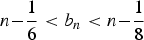
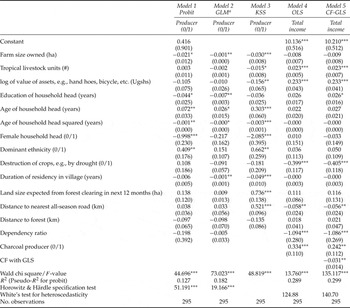
We use equation (2) to identify the factors correlated with charcoal production. For comparison purposes, the first three columns of table 1 report estimates from a probit model (model 1), the ordinal generalized linear model with a probit link function (hereafter, OGLM probit) (model 2) to provide a test of heteroskedasticity (Williams, Reference Williams2010) and a Klein–Spady semi-parametric (KSS) specification (model 3). For reasons mentioned in section 2.1, the discussion of results is based on model 3. To control for problems associated with location and scaling in the semi-parametric specification (see Klein and Spady, Reference Klein and Spady1993), we normalized the dependency ratio to unity. The kernel function was taken as the standard normal density function and we used a bandwidth of 0.4 (i.e., 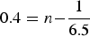 $0.4=n{-{1\over6.5}}$ where n=295).Footnote 8 With only a few exceptions, most of the estimated coefficients for the three specifications (models 1–3) are similar in sign, magnitude and statistical significance. The Horowitz–Härdle (1994) specification test indicates that the ordinary probit function and the OGLM probit might not be appropriate for our data. The test statistic supports rejecting the null hypotheses at a 1 per cent test level.
Regression results for models of charcoal participation and household income

Notes: Figures in parentheses are standard errors. ***, **, * denote estimated parameter is significantly different from zero at the 1%, 5% and 10% test levels, respectively. Note that estimates in model 5 are obtained after bootstrapping with 500 replications to correct the S.E. for the first-stage estimation.
aCoefficients (S.E.) of variables included in variance function are: farm size −0.189** (0.083), household assets −0.463*** (0.155), duration of residency in the village 0.016 (0.021), land size expected from forest clearing 1.686** (0.799), distance to nearest all-season road 2.647** (1.192), and distance to forest 1.748*** (0.638). The choice of variables included in the variance function followed a number of estimations; we first included all variables considered in the table above and the model failed to achieve convergence; we then experimented with a series of different combinations of variables to get a set of variables included in the variance function.
We find that households located farther away from all-season roads (and hence markets) are more likely to participate in charcoal production. Households that are poor in terms of landholdings, livestock and other physical assets are more likely to participate in charcoal production. Presumably, households with large stocks of livestock – particularly cattle – have access to cash and less incentive to participate in charcoal production. Similarly, larger farms provide greater opportunities for both food and cash generation, which also reduce incentives to produce charcoal. To test the life cycle hypothesis, we included age of the household head with its squared term. Younger household heads are more likely to produce charcoal, but as heads grow older, their likelihood of producing charcoal declines. This inverted-U relationship is likely rooted in the physical strength requirements of charcoal production.
Columns 4 and 5 of table 1 report results from two income regressions. Model 4 uses OLS and provides a test for heteroskedasticity. Using White's test for heteroskedasticity we fail to reject the null hypothesis of homoskedascity, but the variance function for the OGLM probit shows that farm size, household assets, amount of land expected from forest clearing in future, distance to the nearest all-season road and distance to the forest are all associated with nonconstant error variance in the participation model of charcoal production. As discussed in section 2.1, having nonconstant error variance in the participation model justifies the analytical strategy proposed for our sample data.
Model 5 employs the CF approach outlined in section 2.1. The main focus in models 4 and 5 is the difference in estimates of the participation coefficients and the CF estimate. The OLS estimate (0.334) is slightly larger than the CF estimate (0.242), but both estimates are significantly different from zero, indicating that unobserved heterogeneity may account for the difference in magnitudes of these estimates. The correlation coefficient on the CF in model 5 is negative and statistically significant, which indicates that participation in charcoal production is endogenous. Comparing estimates in models 4 and 5, the difference in participation estimates not only reflects unobserved heterogeneity, but the correlation coefficient of −0.031 suggests that the returns to this unobserved heterogeneity are negative. Put simply, the unobserved household (and village) heterogeneity that increases the individual's probability to participate in charcoal production is negatively correlated with household income. The economic interpretation is that households that produce charcoal above a certain level (determined by observed characteristics) receive lower returns (due to unobserved heterogeneity) for every increment in charcoal production than households producing below this level. This further suggests that a household may continue to participate in charcoal production up to a certain level conditional on variation in observed characteristics beyond which exit options from charcoal production are likely to be driven by household (and village) unobserved heterogeneity. Results in the next sub-section elaborate on this interpretation.
4.2. The impact of participation in charcoal production on income
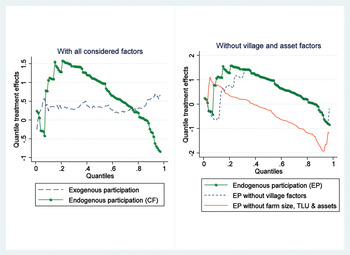
We now turn to estimation of the main results using the analytical procedure described in section 2.1. Figure 1 presents the results. We omit confidence intervals to make the graphs more legible. The left panel of figure 1 compares two measures of the returns to participation in charcoal production. The dashed line is derived assuming participation is exogenously determined. The solid line with dots is derived by computing returns after controlling for endogenous selection into participation, using the CF. The QTEs assuming exogeneity are relatively stable along the distribution up to 80th quantile, beyond which there is a slight increase in the treatment effect. However, when one controls for the endogeneity of participation, returns to participation in charcoal production are much higher and largely positive, but declining gradually along the income distribution, and negative and relatively steep beyond the 85th quantile. This means that returns to charcoal production are high among poor households, but fall as households become better off.
The left panel shows estimation of QTE of participation in charcoal production on income using all considered variables. The right panel shows estimation QTE of participation in charcoal production on income by examining the role of village factors, farm size, livestock (TLU) and other assets. Endogenous quantiles were obtained by bootstrapping with 500 replications

Recalling that the efficiency of the estimates based on equation (5) depends on a set of covariates, the right panel of figure 1 shows how important it is to control for village-level fixed factors and physical assets. The vector of covariates used to achieve efficiency is shown in table 1 (model 5). We use the distribution obtained using all covariates (model 5) as the base distribution. The right panel of figure 1 shows that controlling for village-level fixed factors (distance to all-season road) and household productive assets (land, livestock and other assets) has a modest effect on the derived income distribution. The income distribution deviates considerably from the base distribution when one excludes productive assets, but deviates relatively little when one excludes distance to all-season road, the proxy for market access and remoteness. Overall, these results confirm that the effects of participation vary along the income distribution: they are high at the bottom end and decline gradually toward the top end of the income distribution. To better understand the income advantages that are associated with charcoal production, we now examine whether the observed income gap is due to differences in household characteristics or changes in the economic returns to these household characteristics.
4.3. Decomposition of changes in the income distribution
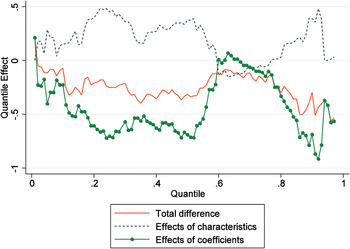
We interpret figure 2 with reference to income gap estimates for endogenous participation in the left panel of figure 1. Recall that the endogenous participation in the left panel of figure 1 presents the income gap between charcoal producers and non-producers based on the propensity score weights. Figure 2 shows the income gap after controlling for differences between charcoal producers and non-charcoal producers in terms of observed household characteristics and returns to these characteristics. That is, figure 2 shows the counterfactual distribution of household income that non-charcoal producers would have obtained, had they possessed the same distribution of household characteristics as the charcoal producers. We use all characteristics considered in model 5.
Decomposition of income gap for charcoal producers and non-charcoal producers with selection term

Contrary to the negative and positive income gaps we observe in figure 1, the total difference curve in figure 2 shows that the income distribution for non-charcoal producers dominates that of charcoal producers, since the income gap is negative for nearly all quantiles. This negative income gap reflects differences in returns to household characteristics. The distribution of returns to household characteristics follows a pattern similar to that of the total difference curve. This means that charcoal producers would earn less income upon exiting charcoal production and it would mostly be disadvantageous for individuals close to both the lower and upper ends of income distribution. However, given the changes in household characteristics (as indicated by the curve labeled ‘effects of characteristics’) in figure 2, the income advantage for charcoal producers over their counterparts is visible for a large part of the lower end of the income distribution – up to around the 59th quantile, after which the income gap is close to zero – and largely negative up to the 76th quantile – beyond which the distribution turns positive again.
What we observe from figures 1 and 2 is that charcoal producers are well off in terms of income compared to non-charcoal producers, largely because of the benefits of participation in charcoal production that arise from higher returns to their household (and village) characteristics. But charcoal producers appear to be at an income disadvantage given returns to their resource endowments compared to non-charcoal producers. We investigate this further via sensitivity analysis, in which we decompose the changes in the distribution of resource endowments for charcoal producers while controlling for selection into charcoal participation.
5. Sensitivity analysis
The analysis that follows builds on the income gap distribution for charcoal producers observed in the left panel of figure 1. If one assumes for the moment that charcoal producers are uniformly poor in terms of assets, then one might reasonably ask why we might observe a large income gap at the lower end of the income distribution that decreases toward the upper end of the income distribution. To answer this question we need to identify which households are stochastically poor (vs. non-poor) and which are structurally poor (vs. non-poor). We follow Carter and May (Reference Carter and May2001) to construct our categories. We define a household as stochastically poor if it is observed to be poor based on its realized household income (H i), but is nevertheless expected to be non-poor given its assets. In other words, a household is stochastically poor if it is poor based on income, but nevertheless possesses assets that collectively place it in a position above the asset poverty line. A household is defined as structurally poor if its assets place it below the asset poverty line. The stochastically and structurally non-poor are defined in a similar way as shown below:
 $$\matrix{Stochastically \ poor \ if \hfill & H_i \lt PL_i\semicolon \; but \ \hat{h}_i\lpar A_i\rpar \gt PL_i \cr Structurally \ poor \ if \hfill & H_i \lt PL_i\semicolon \; and \ \hat{h}_i\lpar A_i\rpar \lt PL_i \cr Stochastically \ non-poor \ if \hfill & H_i \gt PL_i\semicolon \; but \ \hat{h}_i\lpar A_i\rpar \lt PL_i \cr Structurally \ non-poor \ if \hfill & H_i \gt PL_i\semicolon \; and \ \hat{h}_i\lpar A_i\rpar \gt PL_i}$$
where PL i is the poverty line and ĥ i(A i) is expected income given household assets (A i);
 $$H_i =\hat{h}\lpar A_i\rpar +\xi_i$$
where ξi is an error term.
The estimate in (10) is obtained by flexible regression methods so that the marginal contribution of each asset depends on the full bundle of productive assets (A i) controlled by the household. We use polynomial regression of order four to control for any non-linearities that might exist between income and the independent variables.Footnote 9 Explanatory variables used as polynomials include farm size, aggregated value of farm-related assets, and the number of adult-equivalent consumers. Other variables included are tropical livestock units and characteristics of the household head, including education, sex and age. We then use an 80 per cent confidence interval of ĥ i(A i) to allow for a 10 per cent probability of Type I error, that is, that any household that appears to be stochastically poor (non-poor) is not. For example, a household is identified as stochastically poor only if its income level is less than the poverty line and the confidence interval of the expected income ĥ i(A i) given the assets strictly lies above the poverty line.
Table A2 (online appendix) reports the summary of classifications of charcoal producers and non-producers based on observed income and expected income given their assets. We consider only those groups for which we had a reasonable number of observations. Each classification in table A2 is used to construct a counterfactual income distribution. For example, assume that we want to compare the income distribution of structurally non-poor households against that of stochastically non-poor households. Households in both groups are charcoal producers. Denote this classification by C ss. We let C ss be the counterfactual random variable controlling for the household income that a randomly selected household would earn if it were structurally non-poor and participated in charcoal production. Thus, the quantile counterfactual distributions of income are computed as those levels of income that stochastically non-poor households would earn at the τth quantile if the distribution of their characteristics were the same as that of structurally non-poor households. This means that we are decomposing the difference between the structurally non-poor's income (Hstructural) distribution and the stochastically non-poor's income (Hstochastic) distribution, that is, (Hstructural(θ)−Hstochastic(θ)). For ease of interpretation in the subsequent discussion, we refer to the reference classification as the ‘base’. For example, Hstructural references the ‘base’ category.
5.1. Structurally non-poor vs. stochastically non-poor charcoal producers
The online appendix B (which contains all figures for the sensitivity analysis section) presents decomposition results based on the classification in table A2. Figures B2 and B3 (online appendix) decompose the income gap between the structurally non-poor charcoal producers (base) and the stochastically non-poor charcoal producers. Figure B2 presents results without controlling for selection bias (see section 2.2). Figure B3 controls for selection bias. Figure B2 shows that an analysis that ignores selection into participation in charcoal production slightly underestimates the proportion of the income gap between structurally and stochastically non-poor charcoal producers that can be attributed to differences in levels of household characteristics (effect of characteristics). All subsequent discussion is based on results that correct for selection bias.
The estimated total differential shows that the income gap between structurally non-poor charcoal producers and stochastically non-poor charcoal producers is small for a sizeable part of the lower end of the distribution up to about the 50th quantile, beyond which the gap widens considerably toward the upper end of the distribution. This pattern appears to arise from returns to household characteristics. Returns to household characteristics follow a pattern similar to that of the total differential curve. The effects of characteristics slightly dominate in the lower end of the distribution in favor of structurally non-poor charcoal producers. This means that for the least structurally well-off charcoal producers, differences in household characteristics matter more than differences in returns to those characteristics. In contrast, for the most stochastically well-off charcoal producers, returns to household characteristics matter more than differences in household characteristics.
Figure B3 suggests that stochastically non-poor charcoal producers (i.e., those that appear to be non-poor but who would be poor given their assets) benefit more from charcoal production than their structurally non-poor cohorts. Evidence that stochastically non-poor households benefit more from charcoal production than structurally non-poor households supports the overall descriptive results in table A1 and the participation results in table 1, both of which show that charcoal production is a livelihood strategy pursued by relatively young household heads. These young household heads are poor in terms of assets, and charcoal production appears to be a means to accumulate wealth and/or establish grazing areas for their cattle and open land for agricultural production.Footnote 10
5.2. Structurally and stochastically non-poor vs. structurally poor charcoal producers
Figures B4 and B5 (online appendix) decompose the income gaps for structurally and stochastically non-poor charcoal producers (base) compared to structurally poor charcoal producers. In figure B4, differences in distributions of household characteristics appear to play a major role in explaining the income gap for structurally non-poor charcoal producers for a small part of lower income distribution up to about the 10th quantile, beyond which the observed income gap is nearly zero. An almost identical pattern is observed in figure B5. For the stochastically non-poor, differences in household characteristics matter more for explaining the income distribution than difference in returns to these characteristics, at least in the lower end of the income distribution (say, up to about the 25th quantile). In general, the implication is that households in the lower part of income distribution and whose assets place them above the subsistence level have higher incomes than asset-poor households who are also income poor (i.e., the structurally poor).
On the other hand, returns to household characteristics play a larger role in explaining the income gap for structurally poor households. Income differentials are larger at the bottom and upper ends of the distribution than in the middle. This means that both the stochastically and structurally non-poor households would earn less income if the distribution of returns to characteristics were same as that of structurally poor households. These results imply that even though both poor and well-off charcoal producers have similar household characteristics, the income gap is mainly widened by the differences in returns to these household characteristics.
5.3. Structurally poor charcoal producers and structurally poor non-producers
Figure B6 (online appendix) shows the income differential between structurally poor charcoal producers (base) and structurally poor non-charcoal producers. We find that the structurally poor charcoal producers have a fairly large income advantage over the structurally poor non-charcoal producers in the lower end of the income distribution. Beyond the 63rd quantile, the income gap is nearly zero. A large part of this income advantage is explained by differences in household characteristics. However, the opposite effects hold for the structurally poor non-charcoal producers in the same lower half of the income distribution, where the income gap is explained by differences in returns to household characteristics. There are almost no observable differences in household characteristics or their returns, and so the total income differential between these groups is essentially nil in the upper end of the distribution.
5.4. Structurally non-poor charcoal producers and structurally non-poor non-producers
Figure B7 (online appendix) shows the income gap of structurally non-poor charcoal producers (base) and structurally non-poor non-charcoal producers. The income gap associated with differences in household characteristics is negative for a considerable part of the income distribution, with the exception of the quantiles in the neighborhood of the median point (48th to 58th quantiles) and those beyond the 73rd quantile. The negative difference suggests that the structurally non-poor charcoal producers have smaller income advantages over their counterparts conditional on differences in their household characteristics. That is, the negative difference indicates that the structurally non-poor households not engaged in charcoal production would earn less if they switched to producing charcoal. Interestingly, the pattern of income distribution conditional on returns to household characteristics is almost a mirror image of the income distribution based on levels of characteristics. This means that, based on returns to household characteristics, the structurally non-poor households not engaged in charcoal production would earn more if they switched to producing charcoal. This income advantage would largely accrue to households below the mid-point of income distribution. Nevertheless, the overall income gap is stochastic for the most part in the lower half of the income distribution. Beyond the 51st quantile, the gap widens, with the structurally well-off non-charcoal producers earning more from returns to their household characteristics than the structurally non-poor charcoal producers.
5.5. Stochastically non-poor producers and stochastically non-poor non-producers
Finally, figure B8 (online appendix) compares the income gap between stochastically non-poor charcoal producers (base) and stochastically well-off non-charcoal producers. The stochastically non-poor charcoal producers are slightly better off in the lower third of the income distribution (up to the 37th quantile) and worse off throughout the remainder of the income distribution, conditional on their household characteristics. Conditional on returns to their household characteristics, the stochastically well-off non-charcoal producers are worse off in the lower third of the income distribution and better off beyond this point.
6. Conclusions and policy implications
Empirical research continues to support the conjecture that forest utilization is a major livelihood strategy for the rural poor in developing countries, particularly in Africa. Moreover, forests are seen as providing natural insurance against shocks, but potentially perpetuating poverty given the low returns to many NTFPs. In this paper we used data from charcoal producers in Uganda to illustrate that the overall effects of income derived from NTFPs are likely to depend on the characteristics of the households extracting these products.
For some households, we observe that charcoal production has the potential to lift a household out of poverty. Our empirical results confirm previous findings suggesting that younger households and those with few productive agricultural assets are more likely to turn to forests to generate income. Using an approach based on QTE we find that participation in charcoal production has a positive effect on household income. Our findings suggest that households may be using charcoal production in a way that alleviates poverty and opens up options beyond forest dependence. In particular, charcoal producers at the bottom of the income distribution have an income advantage vis-à-vis non-producers, but the advantage narrows as one moves up the income distribution.
When we decomposed the income gap between charcoal producers and non-producers to ascertain whether the observed positive effects of participation in charcoal production are due to differences in household characteristics or returns to these characteristics, we found that charcoal producers are better off in income terms than non-charcoal producers, largely due to high returns to household (and, to some extent, village) characteristics. This compensates for the fact that non-producers tend to have higher levels of productive assets like livestock, landholding and other physical assets.
In sum, asset-poor households that engaged in charcoal production were better off in income terms than asset-poor households that did not produce charcoal. Participation in charcoal production appears to be a temporary means to accumulate income, after which exit from forest product extraction is possible. Future research – preferably with panel data – will need to focus on how returns from commercialized NTFPs are utilized, how environmentally sustainable their use might be under site-specific conditions, and at what point the rural poor might be able to exit from an income-earning strategy based on extraction. Where forest product extraction can be commercialized, NTFPs may emerge as a temporary and intermediate stage in the earning cycle of some rural households, and possibly also in the process of rural development.