


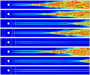

1. Introduction
Boundary transition is common in aeronautical and astronautical systems and is generally accompanied by increases in skin friction drag and aeroheating (Fu & Wang Reference Fu and Wang2013; Zhao et al. Reference Zhao, Wen, Zhou, Tu and Lei2022). The mechanism of transition is complex, and it can occur via different paths and be impacted by different influencing factors. A crucial factor is the surface roughness because it has a significant influence on the transition onset position. Thus, understanding roughness-induced transitions and developing efficient control methods are important topics in fluid dynamics and aerospace science.
The roughness-induced transition is strongly related to the geometry and flow parameters. In particular, the physical height of the roughness element is an important parameter (Schneider Reference Schneider2008). When the roughness height  $k$ is much smaller than the boundary layer thickness
 $\delta$, the roughness is considered small, and the transition is mainly induced by the inherent instability in the boundary layer, such as Tollmien–Schlichting waves (White Reference White2006) and Mack modes (Mack Reference Mack1984), and the small roughness influences only the evolution of these modes. When
 $k/\delta$ is approximately 0.5, the roughness is considered moderate. In this case, the roughness severely distorts the flow profiles and gives rise to the formation of new flow structures. According to previous studies, the typical flow features include flow separation upstream of the roughness, separation shock, a separated shear layer detached from the top of the roughness and a vortex system in the wake region. These different structures may introduce additional instability modes that are absent in an undisturbed boundary layer, resulting in rapid increases in disturbances and ultimately leading to the final breakdown to transition.
Previous studies have investigated the physical mechanisms and dominant instability sources in roughness-induced transitions. In the upstream separation region, a horseshoe vortex is generated around the leading edge of the roughness and then develops into a pair of streamwise vortices in the roughness wake. Separation shock is the main instability source in hypersonic roughness-induced transitional flow past a cylinder-shaped roughness element (Duan & Xiao Reference Duan and Xiao2017), and Subbareddy, Bartkowicz & Candler (Reference Subbareddy, Bartkowicz and Candler2014) noted that the interaction between the upstream vortex and separation shock is also important. The separated shear layer shedding from the top of the roughness element has been found to induce inflection points in the velocity profiles and cause instabilities (Hamed et al. Reference Hamed, Sadowski, Zhang and Chamorro2016). In the roughness flow wake, the counter-rotating vortex pair shedding from the top of the roughness element is an important flow. This pair of vortices strongly rolls up the low-velocity fluids from the wall and thus distorts the boundary layer and bends the separated shear layer. Muppidi & Mahesh (Reference Muppidi and Mahesh2012) noted that the interaction between the separated shear layer and counter-rotating vortex pair triggers disturbances in the shear layer and causes the breakdown to turbulence. Subbareddy et al. (Reference Subbareddy, Bartkowicz and Candler2014) noted that this interaction also contributes substantially to the hypersonic roughness-induced transition. A similar conclusion was reported by Shrestha & Candler (Reference Shrestha and Candler2019): the separated shear layer–counter-rotating vortex pair system is the main reason for the transition past a diamond-shaped roughness.
Stability analysis is an effective tool for further elucidation of the stability characteristics in the roughness wake flow. Using BiGlobal stability analysis and three-dimensional parabolized stability equations, De Tullio et al. (Reference De Tullio, Paredes, Sandham and Theofilis2013) noted that the main instability modes in the wake past a supersonic square roughness are the symmetric (varicose) and the antisymmetric (sinuous) modes, the former showing a higher growth rate and greater amplification. In addition, they noted that symmetric instability is induced by the whole separated shear layer, while antisymmetric instability is related to the spanwise shear layer. Lu et al. (Reference Lu, Zeng, Liu, Liu and Yan2021, Reference Lu, Liu, Zhou and Yan2022b) reported similar results in which symmetric modes dominate the transition for squared roughness in a Mach 2.25 supersonic flow, but the antisymmetric mode is also a reflection of the shear layer rather than only the spanwise component. However, the type of dominant instability is related to the inflow conditions and roughness shape. Balakumar & Kegerise (Reference Balakumar and Kegerise2016) and Lu et al. (Reference Lu, Liu, Sun, Zhou and Yan2022a) reported that the most unstable instability is symmetric when a diamond roughness interacts with two-dimensional inflow disturbances and antisymmetric when the inflow disturbance becomes three-dimensional. For an oblique roughness element at Mach 4.8, Groskopf & Kloker (Reference Groskopf and Kloker2016) noted that the tilt varicose mode shows a larger amplification near the roughness, while the tilt sinuous mode is dominant in the far wake.
In addition to the geometric parameters, the wall temperature is another important factor in transition. Generally, wall heating can destabilize the first mode and stabilize the second mode. For roughness-induced transitions, both Redford, Sandham & Roberts (Reference Redford, Sandham and Roberts2010) and Bernardini, Pirozzoli & Orlandi (Reference Bernardini, Pirozzoli and Orlandi2012), Bernardini et al. (Reference Bernardini, Pirozzoli, Orlandi and Lele2014) found that the transition behaviour depends strongly on the wall temperature. Therefore, they proposed transition maps by correlating the wall temperature with several modified roughness Reynolds numbers. However, they focused mainly on the transition onset positions and criteria and did not discuss how the wall temperature influences the instability modes in the transition processes.
The control of roughness-induced transitions has attracted considerable interest. Several control methods have been proposed for modifying the flow profiles in the wake region. One approach is to place another roughness element behind the first roughness element (Kobayashi et al. Reference Kobayashi, Fukunishi, Nishikawa and Kato1995; Sharma et al. Reference Sharma, Drews, Kuester, Goldstein and White2014; Suryanarayanan et al. Reference Suryanarayanan, Goldstein, Brown, Berger and White2017). Using this method, the distortion caused by the first element in the wake region can be counteracted by the second element. However, this method has the limitation that it requires special roughness geometries. Another method is based on the shielding effect (Kuester et al. Reference Kuester, Sharma, White, Goldstein and Brown2014; Kuester & White Reference Kuester and White2015) by lowering the roughness around the higher roughness. Suryanarayanan et al. (Reference Suryanarayanan, Goldstein, Berger, White and Brown2020) confirmed that the shielding effect can effectively suppress the isolated-roughness-induced transition in subsonic flows. Lu et al. (Reference Lu, Liu, Liu and Yan2020a,Reference Lu, Liu, Liu and Yanb) further analysed the upstream and downstream shielding effects in transonic boundary layers in detail and noted that the upstream and downstream control mechanisms are different. In addition to the above passive control methods, active transition control approaches have been developed. Wall blowing is used to control laminar–turbulent breakdown induced by first-mode disturbance (Sharma et al. Reference Sharma, Shadloo, Hadjadj and Kloker2019; Kneer, Guo & Kloker Reference Kneer, Guo and Kloker2021) and square/diamond-roughness-induced transitions (Lu et al. Reference Lu, Zeng, Liu, Liu and Yan2021, Reference Lu, Liu, Sun, Zhou and Yan2022a). Local wall cooling/heating is another widely used control method. It is reported to have significant influences on first- and second-mode-induced transitions in high-speed flows (Zhao et al. Reference Zhao, Wen, Tian, Long and Yuan2018).
As mentioned above, wall temperature is an important factor that influences roughness-induced transitions. However, there are no relevant studies on whether local wall heating or cooling can control the roughness-induced transition. Therefore, this investigation investigates the roughness-induced transition in a supersonic flow controlled by local wall heating strips using direct numerical simulation (DNS) and BiGlobal linear stability analysis. The study strategy is as follows. We first study the transition mechanism of isolated-roughness-induced transitions in detail and further investigate the effect of wall temperature on transitions. On this basis, local wall heating strips located both upstream and downstream of the roughness zone are studied to identify the differences in the role of transition control, combined with different wall heating temperatures, strip widths and strip locations. Finally, transition control scenarios with different roughness heights, a point-source disturbance hole and different roughness shapes are considered and studied to examine the credibility of the proposed transition control method.
The rest of this paper is arranged as follows. The numerical methods are described in § 2, and the computational details including the set-up of the physics problem and a grid sensitivity study are presented in § 3. The numerical results are then presented and discussed, with the mechanisms for the roughness-induced transition under different wall temperatures in § 4, the transition control mechanisms analysed in § 5 and other transition control cases in § 6. Finally, the study is concluded in § 7.
2. Numerical methods
2.1. Direct numerical simulation
For the present DNS, the governing equation is the fully three-dimensional Navier–Stokes equation for unsteady compressible flows, i.e.
 \begin{equation} \frac{\partial \boldsymbol{Q}}{\partial t}+\frac{\partial \boldsymbol{F}_{j}}{\partial x_{j}}=\frac{\partial \boldsymbol{F}_{{j,\nu}}}{\partial x_{j}}, \end{equation}
where  $t$ is time,
 $x_{j}$ is the Cartesian coordinate in the
 $j$ direction and
 $\boldsymbol {Q}$,
 $\boldsymbol {F}_{j}$ and
 $\boldsymbol {F}_{{j,\nu }}$ represent the vectors of the conserved variables, convective fluxes and viscous fluxes, respectively. These are defined as
 \begin{equation} \boldsymbol{Q}= \begin{bmatrix} \rho \\ \rho u_{i} \\ \rho e \\ \end{bmatrix}, \quad \boldsymbol{F}_{j}= \begin{bmatrix} \rho u_{j}\\ \rho u_{i} u_{j}+p\delta_{ij}\\ \left( \rho e+p \right)u_{j}\\ \end{bmatrix}, \quad \boldsymbol{F}_{{j,\nu}}= \begin{bmatrix} 0\\ \sigma_{ij}\\ \sigma_{ij} u_{i}+q_{j}\\ \end{bmatrix}, \end{equation}
with
 \begin{equation} e=\frac{p}{\left( \gamma-1 \right)\rho}+\frac{u_{i}^{2}}{2}, \quad \sigma_{ij}=\mu\left( \frac{\partial u_{j}}{\partial x_{i}}+\frac{\partial u_{i}}{\partial x_{j}} \right)-\frac{2}{3}\mu \delta_{ij} \boldsymbol{\nabla} \boldsymbol{\cdot} \boldsymbol{u}, \quad q_{j}=\mu\frac{c_{p}}{\Pr}\frac{\partial T}{\partial x_{j}}. \end{equation}
Here,  $\delta _{ij}$ is the Kronecker delta,
 $\boldsymbol {u} = [ u,v,w ]^{T}$ is the velocity vector,
 $p$ is the pressure,
 $\rho$ is the density and
 $c_{p}$ is the specific heat. The viscosity
 $\mu$ is calculated using Sutherland's law. The governing equations are closed by the state equation of a perfect gas. The specific heat ratio
 $\gamma$, gas constant
 $R$ and Prandtl number
 $Pr$ are set to 1.4, 287 and 0.72, respectively. The velocities are non-dimensionalized by the streamwise free-stream velocity
 $u_{\infty }$, and the other variables are non-dimensionalized by the corresponding free-stream values. The reference length is
 $L_{ref}=0.001$ m.
The governing equation is solved on a body-fitted grid using the finite-difference DNS code OpenCFD developed by Li, Fu & Ma (Reference Li, Fu and Ma2010). The third-order Runge–Kutta method (Jiang & Shu Reference Jiang and Shu1996) is used for time advancement. For spatial discretization, the convective flux vectors are computed by a seventh-order WENO-SYMBO scheme (Martín et al. Reference Martín, Taylor, Wu and Weirs2006) with Steger–Warming splitting (Steger & Warming Reference Steger and Warming1981). The viscous flux vectors are computed using the eight-order central difference method.
2.2. BiGlobal linear stability analysis
The flow variables  $\boldsymbol {q}=[\rho, u, v, w, T]^{T}$ can be split into the mean flow
 $\bar {\boldsymbol {q}}$ and the small disturbance
 $\boldsymbol {q}'$, i.e.
 \begin{equation} \boldsymbol{q}(x,y,z,t) =\bar{\boldsymbol{q}}(x,y,z) +\boldsymbol{q}'(x,y,z,t). \end{equation}
By substituting equation (2.4) into the Navier–Stokes equation, subtracting the mean flow and ignoring the nonlinear terms, we obtain the governing equation of the small disturbance, namely the linearized Navier–Stokes (LNS) equation:
 \begin{align} &\boldsymbol{\varGamma}\frac{\partial \boldsymbol{q}'}{\partial t} +\boldsymbol{A}\frac{\partial \boldsymbol{q}'}{\partial x} +\boldsymbol{B}\frac{\partial \boldsymbol{q}'}{\partial y} +\boldsymbol{C}\frac{\partial \boldsymbol{q}'}{\partial z} +\boldsymbol{D}\boldsymbol{q}'\nonumber\\ &\quad =\boldsymbol{H}_{xx}\frac{\partial^{2} \boldsymbol{q'}}{\partial x^{2}}+\boldsymbol{H}_{yy}\frac{\partial^{2} \boldsymbol{q'}}{\partial y^{2}}+\boldsymbol{H}_{zz}\frac{\partial^{2} \boldsymbol{q'}}{\partial z^{2}}+\boldsymbol{H}_{xy}\frac{\partial^{2} \boldsymbol{q'}}{\partial x \partial y}+\boldsymbol{H}_{xz}\frac{\partial^{2} \boldsymbol{q'}}{\partial x \partial z}+\boldsymbol{H}_{yz}\frac{\partial^{2} \boldsymbol{q'}}{\partial y \partial z}, \end{align}
where  $\boldsymbol {\varGamma }$,
 $\boldsymbol {A}$,
 $\boldsymbol {B}$,
 $\boldsymbol {C}$,
 $\boldsymbol {D}$,
 $\boldsymbol {H}_{xx}$,
 $\boldsymbol {H}_{yy}$,
 $\boldsymbol {H}_{zz}$,
 $\boldsymbol {H}_{xy}$,
 $\boldsymbol {H}_{xz}$ and
 $\boldsymbol {H}_{yz}$ are matrices that contain only the base flow variables. The non-zero elements in these matrices are listed in Appendix A.
For a steady flow that changes sharply in the wall-normal and spanwise directions but slowly in the streamwise direction, we obtain its local stability characteristics by introducing the quasi-parallel flow assumption, i.e. the mean flow variation in  $x$ is negligible. Therefore, the small disturbance part can be expressed as
 \begin{equation} \boldsymbol{q}'(x,y,z,t)=\hat{\boldsymbol{q}}(y,z) \,{\rm{e}}^{{{\rm i}} (\alpha x-\omega t)}+{\rm{c.c.}}, \end{equation}
where  $\hat {\boldsymbol {q}}$ is the shape function,
 $\alpha =\alpha _{r}+{\rm {i}}\alpha _{i}$ is the complex streamwise wavenumber,
 $\omega$ is the angular frequency and
 ${\rm {c.c.}}$ is the complex conjugate. The real part
 $\alpha _{r}$ is the streamwise wavenumber and the imaginary part
 $\alpha _{i}$ represents the disturbance's spatial growth rate. The corresponding streamwise wavelength and physical frequency are defined as
 \begin{equation} \lambda_{x}=\frac{2 {\rm \pi}}{\alpha_{r}}, \quad f=\frac{\omega}{2 {\rm \pi}}. \end{equation}
Substituting equation (2.6) into (2.5), the LNS equation reduces to a polynomial eigenvalue problem:
 \begin{equation} (\mathcal{L}_{0}+\alpha \mathcal{L}_{1}+\alpha^{2} \mathcal{L}_{2} )\hat{\boldsymbol{q}}=0, \end{equation}
with
 \begin{equation} \left.\begin{array}{@{}c@{}} \displaystyle \mathcal{L}_{0}=\boldsymbol{D}-{\rm{i}} \omega \boldsymbol{\varGamma}+\boldsymbol{B}\dfrac{\partial}{\partial y}+\boldsymbol{C}\dfrac{\partial}{\partial z}-\boldsymbol{H}_{yy}\dfrac{\partial^{2}}{\partial y^{2}}-\boldsymbol{H}_{zz}\dfrac{\partial^{2}}{\partial z^{2}}-\boldsymbol{H}_{yz}\dfrac{\partial^{2}}{\partial y \partial z},\\ \displaystyle \mathcal{L}_{1}={\rm{i}}\left( \boldsymbol{A}-\boldsymbol{H}_{xy}\dfrac{\partial}{\partial y}-\boldsymbol{H}_{xz}\dfrac{\partial}{\partial z} \right),\\ \mathcal{L}_{1}=\boldsymbol{H}_{xx}. \end{array}\right\} \end{equation}
The above equation is discretized using the fourth-order central difference method in the  $y$ and
 $z$ directions. At the wall, the Dirichlet condition is applied:
 \begin{equation} \hat{u}=\hat{v}=\hat{w}=\hat{T}=0, \quad y=0, \end{equation}
and  $\hat {\rho }$ is solved for directly. A non-reflecting condition (Chang Reference Chang2004) is used in the far field, and a periodic condition is adopted for the two lateral boundaries. By solving this eigenvalue problem at a given frequency
 $\omega$ using the two-level orthogonal Arnoldi algorithm (Zhu Reference Zhu2005), we obtain the complex streamwise wavenumber
 $\alpha$ and the shape function
 $\hat {\boldsymbol {q}}$.
3. Computational detail
The physical problem studied here is a supersonic flow past a smooth-edge isolated roughness element on an isothermal flat plate. The flow parameters mainly refer to the DNS study of Pirozzoli, Grasso & Gatski (Reference Pirozzoli, Grasso and Gatski2004). The free-stream Mach number is  $M_{\infty }=2.25$, the free-stream unit Reynolds number formed with the free-stream density, free-stream velocity and free-stream viscosity is
 $Re_{\infty }=2.5\times 10^{7}\ \textrm {m}^{-1}$ and the free-stream static temperature is
 $T_{\infty }=169.44$ K.
The computational domain is depicted in figure 1. The roughness element has a square shape and is placed at  $x_{r}=101.6$ mm. At this station, the thickness of the laminar flat-plate boundary layer is
 $\delta _{r}=0.444$ mm. The roughness element is defined by the following function:
 \begin{align} y_{r}(x,z)&=\frac{k_{r}}{4}\left\{ \tanh\left[ \sigma\left(\frac{r}{2}-x_{1}\right) \right]+\tanh\left[ \sigma\left(\frac{r}{2}+x_{1}\right) \right]\right\} \nonumber\\ &\quad \times \left\{\tanh\left[ \sigma\left(\frac{r}{2}-z_{1}\right) \right]+\tanh\left[ \sigma\left(\frac{r}{2}+z_{1}\right) \right] \right\}, \end{align}
with
 \begin{equation} x_{1}=(x-x_{r})\cos \alpha-z\sin\alpha, \quad z_{1}=(x-x_{r})\sin\alpha+z\cos\alpha. \end{equation}
Here,  $k_{r}$ is the maximum height of the roughness element and
 $\alpha$,
 $\sigma$ and
 $r$ are shape parameters. In this study, square roughness elements with different heights and a diamond roughness element are considered, and their detailed shape parameters are listed in table 1.
Computational domain.

Shape parameters for two roughness elements.

The computational domain consists of a well-resolved region and a sponge region. The former has a size of  $L_{x} \times L_{y} \times L_{z}=150\delta _{r} \times 28.6\delta _{r} \times 10\delta _{r}$ and the latter has a length of
 $50\delta _{r}$. The inflow domain is at
 $x=x_{r}-50\delta _{r}$. A steady laminar profile is imposed at the inlet boundary. This profile is obtained by solving the following similarity equations for the compressible laminar boundary layer (White Reference White2006):
 \begin{equation} \left. \begin{array}{@{}c@{}} \displaystyle \dfrac{{\rm{d}}}{{\rm{d}}\eta}\left( \dfrac{\rho \mu}{\rho_{\infty} \mu_{\infty}} \dfrac{{\rm{d}}^{2}f}{{\rm{d}}\eta^{2}} \right)+f\dfrac{{\rm{d}}^{2}f}{{\rm{d}}\eta^{2}}=0,\\ \displaystyle \dfrac{{\rm{d}}}{{\rm{d}}\eta}\left( \dfrac{\rho \mu}{\rho_{\infty} \mu_{\infty}} \dfrac{{\rm{d}}g}{{\rm{d}}\eta} \right)+\Pr f \dfrac{{\rm{d}}g}{{\rm{d}}\eta}+\Pr\left( \gamma-1 \right)M_{\infty }^{2}\dfrac{\rho \mu}{\rho_{\infty} \mu_{\infty}}\left( \dfrac{{\rm{d}}^{2}f}{{\rm{d}}\eta^{2}} \right)^{2}=0, \end{array}\right\} \end{equation}
with
 \begin{equation} \frac{{\rm{d}}f}{{\rm{d}} \eta}=\frac{u}{{u}_{\infty}}, \quad g=\frac{T}{T_{\infty}}, \quad \eta =\frac{u_{\infty}}{\sqrt{2\xi }}\int_{0}^{y}\rho\, {\rm{d}}y, \quad \xi =\int_{0}^{x} \rho_{\infty} u_{\infty} \mu_{\infty}\, {\rm d}x \end{equation}
and
 \begin{equation} f(0)=\frac{{\rm{d}}f}{{\rm{d}}\eta} \bigg|_{\eta=0}=0, \quad g(0)=\frac{T_{w}}{T_{\infty}}, \quad \lim_{\eta \rightarrow +\infty}\frac{{\rm{d}}f}{{\rm{d}}\eta}=\lim_{\eta \rightarrow +\infty} g=1. \end{equation}
At the outflow domain, a supersonic outlet boundary (Pirozzoli et al. Reference Pirozzoli, Grasso and Gatski2004) is applied: second-order extrapolation is imposed for all variables except in the subsonic region of the boundary layer, where the pressure is set as the value of the first grid point where the local Mach number is greater than one. For the upper far-field boundary, a non-reflecting boundary condition (Pirozzoli et al. Reference Pirozzoli, Grasso and Gatski2004) is imposed. Periodic conditions are set for the two lateral domains.
The wall is set to be isothermal, and different wall temperatures and upstream or downstream wall heating control strips are considered. Within the control strip, the wall temperature  $T_{w}$ is set to a constant value; in the control strip, the wall temperature is set as the heating temperature
 $T_{strip}$. The control strip is placed at different locations (
 $x_{strip}$), and its width is
 $L_{strip}=10k_{r}$ or
 $20 k_{r}$. In addition, the heating temperature
 $T_{strip}$ is also a factor considered in this study. The detailed flow parameters for all cases considered in this study are tabulated in table 2. Here, the wall temperature and heating strip temperature are expressed as the ratio of the wall temperature to the turbulence adiabatic wall temperature
 $T_{aw} = 322$ K (same as in Pirozzoli et al. (Reference Pirozzoli, Grasso and Gatski2004) and Lu et al. (Reference Lu, Zeng, Liu, Liu and Yan2021)), which is computed according to
 $T_{aw}=T_{\infty }[ 1+r_{turb} (\gamma -1) M_{\infty }^{2}/2 ]$, with
 $r_{turb}=0.89$ being the turbulent recovery factor.
Details of all cases in this paper.

The naming scheme for the cases is described below. The first character indicates the type of roughness element: S (square) and D (diamond). In the cases without control strips, this first character is followed by a subscript that represents the temperature of the wall. In the transition control cases, the subscript of the first character indicates the location of the control strip. The second character L and its subscript denote the width of the control strip. The third character T and its subscript describe the heating temperature of the control strip. Then, the naming string is terminated, trailed by a character  $L$ (indicating the lower roughness height
 $k_{r}=0.122$ mm), trailed by a character
 $H$ (indicating the higher roughness height
 $k_{r}=0.133$ mm) or trailed by a character
 $P$ (indicating the unsteady point source wall disturbance).
In this study, a multi-frequency point source is used to excite a wide spectrum of disturbances through a blowing–suction hole on the wall. This disturbance hole takes the form of (Groskopf & Kloker Reference Groskopf and Kloker2016; Kneer et al. Reference Kneer, Guo and Kloker2021)
 \begin{equation} \rho v=A_{dis} \varTheta(x,z) \sum_{m=1}^{M} \cos \left(\frac{m}{8} \omega_{0} t\right), \end{equation}
with
 \begin{align} \varTheta(x,z)={-}3\left[ 1-\frac{\sqrt{(x-x_{c})^{2}+ (z-z_{c})^{2}}}{R_{dis}} \right]^{4}+4\left[ 1-\frac{\sqrt{(x-x_{c})^{2}+(z-z_{c})^{2}}}{R_{dis}} \right]^{3}, \end{align}
where  $A_{dis}$ is the disturbance amplitude,
 $M$ is the number of disturbances and
 $\omega _{0}$ is the fundamental angular frequency. In this study,
 $A_{dis}=0.002$,
 $M=50$ and
 $\omega _{0}=1703$ kHz are used. The choice of
 $\omega _{0}$ is shown in detail in § 6.2. The disturbance hole is centred at
 $(x_{c},z_{c})$ with
 $x_{c}-x_{r}=-40\delta _{r}$ and
 $z_{c}=0$. The radius of the hole is
 $R_{dis}=4k_{r}$.
In all cases, the grid resolution for the well-resolved region is  $\Delta x_{max}^+ \times \Delta y_{w}^+ \times \Delta z_{max}^+=14.5 \times 0.95 \times 6.5$. In the roughness and heating strip regions, the streamwise grid is further refined to
 $\Delta x^+=6.4$ to better simulate the flow field. The grid numbers for all cases are also shown in table 1. The grid resolution in this study is basically the same as those used in the DNS of a turbulent boundary layer by Pirozzoli et al. (Reference Pirozzoli, Grasso and Gatski2004) and Li et al. (Reference Li, Fu, Ma and Gao2009), and it is much finer than that of the DNS of oblique-mode breakdown transition by Sharma et al. (Reference Sharma, Shadloo, Hadjadj and Kloker2019) (see table 3). A fine grid with
 $\Delta x_{max}^+ \times \Delta y_{w}^+ \times \Delta z_{max}^+=7.5 \times 0.85 \times 5.5$ and
 $n_{x} \times n_{y} \times n_{z}=2480\times 122\times 304$ is used to evaluate the grid sensitivity. Figure 2(a) plots the time- and spanwise-averaged skin friction coefficient
 $C_{f}$ for cases
 $S_{1.0}$ and
 $S_{1.0, {fine}}$. The DNS results from Lu et al. (Reference Lu, Zeng, Liu, Liu and Yan2021) and the empirical correlation of White (Reference White2006) for the fully turbulent boundary layer are shown for reference:
 \begin{equation} C_{f}=\frac{0.455}{S^{2}}\ln^{{-}2}\left[ \frac{0.06}{S} Re_{\infty} x \frac{\mu_{\infty}}{\mu_{w}} \sqrt{\frac{T_{\infty}}{T_{w}}}\right], \end{equation}
with
 $$\begin{gather} S=\frac{\sqrt{T_{aw}/T_{\infty}-1}}{\arcsin(A)+\arcsin(B)}, \end{gather}$$
 $$\begin{gather}A=\frac{2a^{2}-b}{\sqrt{4a^{2}+b^{2}}},
\quad
B=\frac{b}{\sqrt{4a^{2}+b^{2}}},
\end{gather}$$
 $$\begin{gather}a=\sqrt{\frac{\gamma-1}{2}M_{\infty}^{2}\frac{T_{\infty}}{T_{w}}}, \quad b=\frac{T_{aw}}{T_{w}}-1. \end{gather}$$
From the comparison, we can see that the  $C_{f}$ distributions in cases
 $S_{1.0}$ and
 $S_{1.0,{fine}}$ only have slight differences, and are both in good agreement with the reference value of Lu et al. (Reference Lu, Zeng, Liu, Liu and Yan2021). In the turbulent region, the DNS results correspond well to the empirical correlation. In addition, the width of the computational domain
 $L_{z}$ is referenced to the study of Pirozzoli et al. (Reference Pirozzoli, Grasso and Gatski2004) and Lu et al. (Reference Lu, Zeng, Liu, Liu and Yan2021). To verify whether
 $L_{z}$ is sufficiently large, two-point correlation in the spanwise direction is analysed. The correlation coefficient for a quantity
 $q$ is defined as (Pirozzoli et al. Reference Pirozzoli, Grasso and Gatski2004)
 \begin{equation} R_{qq}( L_{c} )=\sum_{k=1}^{n_{z}-1}\overline{q'_{k}q'_{k+k_{c}}}, \quad k_{c}=0,1,\ldots,n_{z}-1, \end{equation}
where  $L_{c}=k_{c}L_{z}/n_{z}$ is the distance between two points. Figure 2(b) plots the correlation coefficients at
 $y=k_{r}$ and two different streamwise locations
 $x-x_{r}=60\delta _{r}$ or
 $95\delta _{r}$. The correlation coefficients for
 $u$,
 $v$ and
 $w$ at the two positions decrease rapidly within
 $L_{c}<0.1L_{z}$ and approach nearly zero beyond that distance. This means that the two-point correlation functions are sufficiently decorrelated over a distance
 $L_{z}/2$, thus ensuring that the computational domain in the spanwise direction is sufficiently wide to capture the flow fluctuation. Overall, the results confirm that the current grid resolution, computational domain and numerical methods are accurate enough to simulate the roughness-induced transition process.
Summary of the grid resolution and sensitivity study.

Results of (a) validation and grid sensitivity study and (b) spanwise correlation coefficients at  $y=k_{r}$ for case
 $S_{1.0}$.

4. Mechanisms for the square roughness-induced transition
4.1. General flow features
The typical flow features in roughness-induced transitions were investigated through case  $S_{1.0}$. Figures 3(a) and 3(b) plot the instantaneous
 $u$ at
 $y=0.5k_{r}$ and the time-averaged
 $C_{f}$ at the wall, respectively. From the velocity contours, we can find two evident high-speed streaks past the roughness element. The streaks first remain stable until they begin to break down at
 $x-x_{r} \approx 22 \delta _{r}$. Then, high-speed patterns appear in the streaks as well as in the low-speed region between the streaks. As the flow develops further downstream, the high-speed region expands in the spanwise direction, and a clear turbulent wedge appears. From the averaged
 $C_{f}$ contours, the roughness element first induces a high-wall-shear region. In the roughness wake region, the
 $C_{f}$ distribution exhibits a behaviour similar to that of the velocity distribution. The wall shear in the two streaks is greater. As the flow develops to the breakdown position,
 $C_{f}$ sharply increases and gradually expands in the spanwise direction.
(a) Instantaneous streamwise velocity at  $y=0.5 k_{r}$ and (b) time-averaged skin friction coefficient
 $C_{f}$ at the wall for case
 $S_{1.0}$.

According to previous studies (De Tullio et al. Reference De Tullio, Paredes, Sandham and Theofilis2013; Lu et al. Reference Lu, Zeng, Liu, Liu and Yan2021), the roughness-induced transition at a supersonic Mach number is mainly induced by the instabilities in the wake region. Figure 4 shows different cross-stream slices in the wake region of case  $S_{1.0}$. Here, the contours of the
 $Q$ criterion are plotted, which is defined as
 \begin{equation} Q={-}\frac{1}{2}\left[\left(\frac{\partial u}{\partial x}\right)^{2}+\left(\frac{\partial v}{\partial y}\right)^{2}+\left(\frac{\partial w}{\partial z}\right)^{2}\right]-\frac{\partial u}{\partial y}\frac{\partial v}{\partial x}-\frac{\partial u}{\partial z}\frac{\partial w}{\partial x}-\frac{\partial v}{\partial z}\frac{\partial w}{\partial y}, \end{equation}
with the reference value  $Q_{ref}=u_{\infty }^{2}/L_{ref}^{2}$. At
 $x-x_{r}=6\delta _{r}$, we observe two pairs of vortices. The pair on the outside is the horseshoe vortex that is formed by the side of the roughness. The pair closest to the
 $z=0$ plane is the counter-rotating vortex created by the separated shear layer above the roughness. The
 $Q$ criterion states that the counter-rotating vortex is much stronger than the horseshoe vortex. The isolines of the streamwise velocity indicate that the boundary layer is strongly distorted by the counter-rotating vortex and is concentrated on the top region of the roughness element. The isolines of local shear, which is defined as
 \begin{equation} u_{s}=\sqrt{\left(\frac{\partial u}{\partial y}\right)^{2}+\left(\frac{\partial u}{\partial z}\right)^{2}}, \end{equation}
show that the distorted boundary layer generates a strong shear layer above the roughness element, and slight velocity fluctuations are observed in this region. As the flow develops downstream, the strength of the vortices decreases, and the boundary layer distortion also decreases; the separated shear layer remains strong and is gradually bent by the counter-rotating vortex. Moreover, the velocity fluctuations become much stronger, and the resulting distribution is highly consistent with that of the high-shear region. This phenomenon indicates that the interaction between the separated shear layer and counter-rotating vortex generates a high-shear region above the roughness element, thus leading to an increase in disturbance amplitude.
Slices of case  $S_{1.0}$ at (a,b)
 $x-x_{r}=6\delta _{r}$, (c,d)
 $x-x_{r}=10\delta _{r}$ and (e,f)
 $x-x_{r}=14\delta _{r}$ coloured by (a,c,e)
 $Q$ criterion and (b,d,f) streamwise velocity fluctuation. The grey solid curves in (a,c,e) and (b,d,f) are isolines of streamwise velocity and local shear value, respectively. The black dashed curve is the outline of the roughness element.

To further investigate the instability in the roughness wake region, spectral analysis was used. As shown in figure 4, six different probes are adopted in the flow field to record the flow fluctuation, where probes 1, 3 and 5 are placed in the core of the counter-rotating vortex and probes 2, 4 and 6 are placed in the high-shear region at the  $z=0$ plane. Figure 5 shows the spectral analysis results of the streamwise velocity fluctuations at these probes. Here, the dimensional physical frequency is non-dimensionalized to the Strouhal number St based on
 $u_{\infty }$ and
 $L_{ref}$. The six probes clearly confirmed the presence of a dominant mode with
 $St=0.462$ (
 $f=271$ kHz). This phenomenon further indicates that the dominant instability in the roughness wake results from the combination of the counter-rotating vortex and the separation shear layer.
The spectral analysis results of streamwise velocity fluctuation at (a) probes 1, 3 and 5 and (b) probes 2, 4 and 6 for case  $S_{1.0}$.

BiGlobal linear stability analysis was then applied to case  $S_{1.0}$. In this study, the computational grid for BiGlobal analysis is the same as that used for DNS. Figure 6 shows the instability characteristic at
 $x-x_{r}=10\delta _{r}$ with the dominant frequency
 $St=0.462$. Figure 6(a) plots a part of the eigenvalue spectrum. We can observe two evident unstable modes (marked by red and blue), and the real part of the shape function of the streamwise velocity (
 $\hat {u}_{r}$) is shown for the two modes in figures 6(b) and 6(c), respectively. For the mode in figure 6(b), the growth rate
 $-\alpha _{i}$ is large, and its shape function
 $\hat {u}_{r}$ shows a symmetric pattern with respect to the
 $z=0$ plane. For the mode in figure 6(c), the growth rate
 $-\alpha _{i}$ is low, and its shape function
 $\hat {u}_{r}$ shows an antisymmetric pattern with respect to the
 $z=0$ plane. In addition, the distributions of the two modes are located above the roughness element, corresponding to the distributions of velocity fluctuations and the high-shear region in figure 4(d).
BiGlobal analysis results at  $x-x_{r}=10\delta _{r}$ with
 $St=0.462$ for case
 $S_{1.0}$: (a) eigenvalue spectrum and the real part of the shape function
 $\hat {u}$ for the (b) symmetric mode and (c) antisymmetric mode. The grey solid curves are isolines of the streamwise velocity. The black dashed curve is the outline of the roughness element.

Figure 7 further plots the growth rate and amplification factor  $N$ at different streamwise positions and frequencies. Here, the
 $N$ factor is calculated integrally in the streamwise direction for each frequency
 $St$ as (Groskopf & Kloker Reference Groskopf and Kloker2016)
 \begin{equation} N(St,x)=\int_{x_{0}}^{x}-\alpha_{i}(x)\, {\rm{d}} x, \end{equation}
where  $x_{0}$ is the start position for the integration. This operation is similar to that of the traditional linear stability theory and has also been used in BiGlobal analysis of roughness-induced transitions (Groskopf & Kloker Reference Groskopf and Kloker2016). For the symmetric mode, its maximum growth rate is approximately
 $-\alpha _{i}L_{ref}\approx 1.1$ and is located in the region
 $5.5\delta _{r}< x-x_{r}<7.5\delta _{r}$ with
 $0.49< St<0.58$. For the antisymmetric mode, the maximum growth rate is only approximately 0.3. In addition, the antisymmetric mode becomes stable at
 $x-x_{r}>18\delta _{r}$. This phenomenon indicates that the symmetric mode has a higher growth rate and a wider unstable region than the antisymmetric mode. The maximum amplification factor of the symmetric mode exceeds 6 at
 $x-x_{r}>21\delta _{r}$ within
 $0.41< St<0.51$. However, because of the much lower growth rate, the
 $N$ factor of the antisymmetric mode is lower than that of the symmetric mode at the same streamwise location and frequency. Because the antisymmetric mode is almost stable at
 $x-x_{r}>16\delta _{r}$, the amplification factor in this region has almost no growth. The above analysis further confirms that the symmetric mode is much stronger than the antisymmetric mode and is therefore responsible for the final transition to turbulence.
(a,b) Growth rate and (c,d) amplification factor of the (a,c) symmetric mode and (b,d) antisymmetric mode at different frequencies and streamwise positions for case  $S_{1.0}$.

Through the amplification factor, we can determine the most unstable mode, which has the maximum  $N$ factor. Figure 8 shows the growth of the streamwise velocity fluctuation from DNS and compares it with the most unstable symmetric (
 $St=0.477$,
 $f=280$ kHz) and antisymmetric (
 $St=0.366$,
 $f=215$ kHz) modes. The amplitude of the symmetric mode is clearly much larger than that of the antisymmetric mode and shows much better agreement with the DNS. In addition, the most unstable frequency identified by BiGlobal analysis is very close to that identified by the spectral analysis. Overall, the above results indicate that BiGlobal linear stability analysis can simulate the evolution of the instability in the wake region with reasonable accuracy.
Comparison of streamwise velocity fluctuation amplitudes between DNS and symmetric and antisymmetric modes from BiGlobal analysis for case  $S_{1.0}$.

4.2. Wall temperature effects
The wall temperature effect is studied through comparisons between cases  $S_{0.9}$,
 $S_{1.1}$ and
 $S_{1.2}$. Figure 9(a–d) first shows the general instantaneous flow features for the three cases. For examining if the transition occurs in case
 $S_{1.2}$, the computation is performed on a longer well-resolved domain with
 $L_{x}=310 \delta _{r}$ and
 $n_{x}=3240$, and the sizes and grid numbers in wall-normal and spanwise directions are not changed. Note that figure 9(d) is the spatial continuation of figure 9(c).
Instantaneous streamwise velocity at  $y=0.5k_{r}$ for (a) case
 $S_{0.9}$, (b) case
 $S_{1.1}$ and (c,d) case
 $S_{1.2}$ and time- and spanwise-averaged (e) skin friction coefficient and ( f) momentum thickness Reynolds number.

Clearly, compared to case  $S_{1.0}$, a lower wall temperature results in an earlier transition to turbulence, while a higher wall temperature significantly delays the transition. For case
 $S_{0.9}$, the streaks become stronger and quickly break down at
 $x-x_{r} \approx 15 \delta _{r}$. For case
 $S_{1.1}$, the strength of the streaks decreases, and the breakdown position moves downstream to
 $x-x_{r}\approx 45\delta _{r}$. When
 $T_{w}$ increases to
 $1.2 T_{aw}$ in case
 $S_{1.2}$, the high-speed streaks further weaken and remain steady in the short computational domain, and the breakdown finally occurs at
 $x-x_{r}\approx 190\delta _{r}$. Figure 9(e,f) further plots the time- and spanwise-averaged
 $C_{f}$ and momentum thickness Reynolds number
 $Re_{\theta }$ for these cases. It is clear that as the wall temperature increases, the transition onset position is delayed significantly. Taking case
 $S_{1.0}$ as the baseline, the transition onset in case
 $S_{0.9}$ moves upstream by approximately
 $7\delta _{r}$ and that in case
 $S_{1.1}$ moves downstream by approximately
 $15\delta _{r}$. In case
 $S_{1.2}$, we scale the horizontal axis to display the complete distribution of
 $C_{f}$ (see the green label). Obviously,
 $C_{f}$ exhibits laminar behaviour in a long distance until it begins to increase sharply at
 $x-x_{r}\approx 190\delta _{r}$. A similar phenomenon is shown by the distribution of
 $Re_{\theta }$. However, the rapid increase in
 $Re_{\theta }$ occurs slightly later than that in
 $C_{f}$, indicating that the growth of the boundary layer lags the increase in skin friction.
The reason why an increasing wall temperature can suppress the transition is discussed below. Figure 10 shows the streamwise velocity on the  $z=0$ plane in the upstream region of the roughness. Obviously, with a higher wall temperature, the inflow boundary layer is lifted. Using the flow variables computed by the similarity equations (White Reference White2006), we can compute the roughness Reynolds number
 $Re_{k}=\rho _{k} U_{k} k_{r}/\mu _{k}$. Here, the subscript
 $k$ represents the quantity measured at
 $y=k_{r}$ in a smooth laminar boundary layer. For cases
 $S_{0.9}$,
 $S_{1.0}$,
 $S_{1.1}$ and
 $S_{1.2}$,
 $Re_{k}$ are 522, 420, 342 and 282, respectively. This phenomenon shows that a heating wall can significantly reduce the roughness Reynolds number and suppress the transition. In addition, the streamlines in figure 10(b,d,f) show that a heating wall weakens the vortex system upstream of the roughness, and the separation region also decreases.
Streamwsie velocity and streamlines on the  $z=0$ plane: (a,b) case
 $S_{0.9}$, (c,d) case
 $S_{1.0}$ and (e,f) case
 $S_{1.1}$.

The changes in the roughness wake region are shown in figure 11. A comparison between cases  $S_{0.9}$ and
 $S_{1.1}$ shows that a higher wall temperature significantly weakens the strength of the horseshoe and counter-rotating vortex pairs in the wake region, reducing the boundary layer distortion. Thus, the local shear strength decreases substantially, indicating that the strength of the separated shear layer decreases. As discussed in § 4.1, the transition induced by the roughness element is mainly caused by the interaction between the vortex system and separated shear layer; therefore, a higher wall temperature may suppress the instabilities in the roughness region and delay the transition.
Slices of (a,c) case  $S_{0.9}$ and (b,d) case
 $S_{1.1}$ at (a,b)
 $x-x_{r}=6\delta _{r}$ and (c,d)
 $x-x_{r}=10\delta _{r}$ coloured by the
 $Q$ criterion. The grey solid curves on the left half are isolines of the streamwise velocity and the black solid curves on the right half are isolines of the local shear value. The black dashed curve is the outline of the roughness element.

Using BiGlobal linear stability analysis, the neutral curves of the symmetric and antisymmetric modes at  $x-x_{r}=10\delta _{r}$ are plotted in figure 12(a). Obviously, compared with the baseline case
 $S_{1.0}$, a lower wall temperature in case
 $S_{0.9}$ results in a higher growth rate and wider unstable region for the symmetric and antisymmetric modes. However, a higher wall temperature significantly suppresses the unstable modes. For cases
 $S_{1.1}$ and
 $S_{1.2}$, for the symmetric mode, the growth rate decreases, and the unstable region is narrowed. The antisymmetric mode is fully suppressed and becomes fully stable. In addition, as
 $T_{w}$ increases, the neutral curve moves towards the low-frequency region. The frequency of the disturbance with the largest growth rate also decreases significantly. The distributions of
 $\hat {u}_{r}$ are illustrated in figure 12(b–e) for the disturbance with the largest growth rate at
 $x-x_{r}=10\delta _{r}$. Although the wall temperature changes, the shape of the unstable modes changes little compared with that in the baseline case
 $S_{1.0}$. The peak disturbance is still located in the separated shear layer region above the roughness element. This phenomenon indicates that varying the wall temperature does not change the type of dominant instability but rather only influences the growth rate and the unstable region.
BiGlobal results for cases with different wall temperatures at  $x-x_{r}=10\delta _{r}$. (a) Neutral curves and (b–e) the real part of the shape function
 $\hat {u}$: (b) symmetric mode at
 $St=0.680$ in case
 $S_{0.9}$, (c) antisymmetric mode at
 $St=0.680$ in case
 $S_{0.9}$, (d) symmetric mode at
 $St=0.407$ in case
 $S_{1.1}$ and (e) symmetric mode at
 $St=0.264$ in case
 $S_{1.2}$. The grey solid curves are isolines of the streamwise velocity. The black dashed curve is the outline of the roughness element.

5. Basic transition control cases
5.1. Upstream control
Having obtained an understanding of the flow features of the roughness-induced transition and the main instability characteristics in the roughness wake region, as well as the wall temperature effect on the transition, we now focus on transition control through upstream and downstream wall heating strips. Figure 13(a–e) depicts the instantaneous streamwise velocity distributions for cases with upstream control effects. We find that with the upstream wall heating effect, the high-speed streaks in the wake region remain stable over a longer distance compared with those in case  $S_{1.0}$. In case
 $S_{-6}L_{10}T_{2.0}$, with a control strip that has a width of
 $L_{strip}=10k_{r}$ and a heating temperature of
 $T_{strip}=2.0T_{aw}$, the breakdown of the wake moves downstream to
 $x-x_{r} \approx 30 \delta _{r}$. In case
 $S_{-6}L_{10}T_{2.5}$, as the temperature of the heating strip increases to
 $T_{strip}=2.5T_{aw}$, the transition is further delayed to
 $x-x_{r} \approx 34 \delta _{r}$. In case
 $S_{-6}L_{20}T_{2.0}$, the width of the strip increases to
 $L_{strip}=20\delta _{r}$, and the transition moves further downstream to
 $x-x_{r} \approx 36\delta _{r}$ compared with that in case
 $S_{-6}L_{10}T_{2.0}$. In addition, the effect of the location of the control strip was also studied. In cases
 $S_{-10}L_{10}T_{2.0}$ and
 $S_{-10}L_{20}T_{2.0}$, although the control strip has been moved upstream to
 $x_{strip}-x_{r}=-10\delta _{r}$, the transition scenario shows only slight differences compared with cases
 $S_{-6}L_{10}T_{2.0}$ and
 $S_{-6}L_{20}T_{2.0}$, respectively. The above comparison shows that the transition suppression is enhanced with a wider control strip or a higher control temperature, and the location of the control strip weakly influences the transition control effect. Figures 13( f) and 13(g) plot the time- and spanwise-averaged
 $C_{f}$ and
 $Re_{\theta }$ for the cases with upstream control strips, respectively. Generally, the comparison of
 $C_{f}$ shows that the upstream wall heating strip can suppress the transition, but the suppression effect is not very significant, and the flow develops to full turbulence in all the cases. The suppression effect is enhanced with increasing heating temperature and width of the control strip. The location of the upstream control strip has little effect on the transition onset position. The evolution of
 $Re_{\theta }$ has a similar tendency to that of
 $C_{f}$.
Instantaneous streamwisse velocity at  $y=0.5 k_{r}$ for (a) case
 $S_{-6}L_{10}T_{2.0}$, (b) case
 $S_{-6}L_{10}T_{2.5}$, (c) case
 $S_{-6}L_{20}T_{2.0}$, (d) case
 $S_{-10}L_{10}T_{2.0}$ and (e) case
 $S_{-10}L_{20}T_{2.0}$ and time- and spanwise-averaged ( f) skin friction coefficient and (g) momentum thickness Reynolds number.

The flow fields in the wake region are plotted in figure 14. Compared with the baseline case  $S_{1.0}$, the main flow structure of the wake changes slightly with the upstream wall heating strip in case
 $S_{-6}L_{10}T_{2.0}$. However, the vortex system and separation shear layer become weaker. The distortion of the flow profile and the velocity fluctuations are also diminished. As the heating temperature or width of the control strip increases, the strength of the wake structure further decreases. Therefore, the interaction between the separation shear layer and counter-rotating vortex is suppressed, and the instabilities in the wake region are suppressed as well. As the transition is induced by the instabilities in the wake region, the transition is delayed by the upstream wall heating strip.
Slices of (a,b) case  $S_{-6}L_{10}T_{2.0}$, (c,d) case
 $S_{-6}L_{10}T_{2.5}$ and (e,f) case
 $S_{-6}L_{20}T_{2.0}$ at
 $x-x_{r}=10\delta _{r}$ coloured by (a,c,e)
 $Q$ criterion and (b,d,f) streamwise velocity fluctuation. The grey solid curves in (a,c,e) and (b,d,f) are isolines of streamwise velocity and local shear value, respectively. The black dashed curve is the outline of the roughness element.

Compared with the cases with a whole heating wall, the upstream wall heating strip does not directly influence the flow structures in the roughness wake region but rather influences the inflow boundary layers. Figure 15 plots the streamwise velocity distributions in the  $z=0$ plane. The upstream wall heating strip can directly lift up the inflow, thereby decreasing
 $Re_{k}$ and weakening the flow structure in the wake region. In addition, upstream wall heating strips can weaken the flow separation in front of the roughness element. Using DNS of the upstream wall heating strip but without the roughness element, the flow parameters at
 $x=x_{r}$ and
 $y=k_{r}$ are listed in table 4. These parameters reveal that the local Mach number, density and streamwise velocity decrease with increasing temperature. This variation results in a lower
 $Re_{k}$. In addition,
 $Re_{k}$ in cases
 $S_{-6}L_{10}T_{2.0}$ and
 $S_{-10}L_{10}T_{2.0}$ only have a slight difference, and the difference between cases
 $S_{-6}L_{20}T_{2.0}$ and
 $S_{-10}L_{20}T_{2.0}$ is a little more obvious. However, these data are extruded from undisturbed laminar boundary layer profiles; in the actual transition cases, the roughness element will hinder the development of the flow and therefore the situation will be a little different.
Streamwise velocity and streamlines in the  $z=0$ plane: (a,b) case
 $S_{1.0}$, (c,d) case
 $S_{-6}L_{10}T_{2.0}$ and (e,f) case
 $S_{-6}L_{20}T_{2.0}$.

Parameters of upstream control cases at  $x=x_{r}$ and
 $y=k_{r}$ in an undisturbed laminar boundary layer.

To further investigate the effect of upstream wall heating on the instability in the roughness wake region, BiGlobal linear stability analysis was performed. Figure 16 shows part of the eigenvalue spectrum for cases  $S_{-6}L_{10}T_{2.0}$,
 $S_{-6}L_{10}T_{2.5}$ and
 $S_{-6}L_{20}T_{2.0}$ at
 $x-x_{r}=10\delta _{r}$ with
 $St=0.462$. In case
 $S_{-6}L_{10}T_{2.0}$, we can still observe two obvious unstable modes, namely the symmetric (marked in blue) and antisymmetric (marked in red) modes. However, compared with the results of case
 $S_{1.0}$ in figure 6(a), the growth rate
 $-\alpha _{i}$ significantly decreases and the streamwise wavenumber
 $\alpha _{r}$ increases slightly. In case
 $S_{-6}L_{10}T_{2.5}$, as the heating temperature increases, the growth rate of the symmetric mode further decreases, and the antisymmetric mode vanishes. In case
 $S_{-6}L_{20}T_{2.0}$, the width of the strip increases, the symmetric mode is also suppressed and the antisymmetric mode vanishes. This phenomenon indicates that the upstream wall heating strip can effectively suppress both the symmetric and antisymmetric modes.
Eigenvalue spectrum at  $x-x_{r}=10\delta _{r}$ with
 $St=0.462$ for (a) case
 $S_{-6}L_{10}T_{2.0}$, (b) case
 $S_{-6}L_{10}T_{2.5}$ and (c) case
 $S_{-6}L_{20}T_{2.0}$.

The results for the growth rate and amplification factor for the symmetric mode are presented in figure 17. Compared with the results for case  $S_{1.0}$ in figure 7(a), the maximum growth rate in case
 $S_{-6}L_{10}T_{2.0}$ is significantly lower, but the unstable region becomes larger. In case
 $S_{-6}L_{10}T_{2.5}$, as
 $T_{strip}$ increases to 2.5
 $T_{aw}$, the maximum growth rate is further suppressed, but the symmetric mode maintains a growth rate of
 $-\alpha _{i}L_{ref}\approx 0.4$ for a long distance. In case
 $S_{-6}L_{20}T_{2.0}$,
 $L_{strip}$ increases to
 $20k_{r}$; however, although the maximum growth rate further decreases, the symmetric mode still has a clearly unstable growth rate over a long distance. From the distributions of the amplification factor, its maximum value for the cases with upstream control strips achieves a similar level of approximately 5–5.5 before the final breakdown to turbulence. In addition, the unstable mode with the largest growth rate or amplification factor is shifted to the lower-frequency region compared with the case
 $S_{1.0}$.
(a–c) Growth rate and (d–f) amplification factor for the symmeyric mode of (a,d) case  $S_{-6}L_{10}T_{2.0}$, (b,e) case
 $S_{-6}L_{10}T_{2.5}$ and (c,f) case
 $S_{-6}L_{20}T_{2.0}$ at different frequencies and streamwise positions.

As discussed by De Tullio et al. (Reference De Tullio, Paredes, Sandham and Theofilis2013), the growth of the symmetric mode is mainly due to the wall-normal and spanwise components of the local shear layer. To analyse this effect, the contributions of the wall-normal and spanwise shear components to the production of the disturbance kinetic energy in the cases with upstream wall heating strips are analysed. The production term is computed as
 \begin{equation} P=\overbrace{-\bar{\rho}{\rm Re}(\hat{u}\hat{v}^{{{\dagger}}})\frac{\partial \bar{u}}{\partial y}}^{P_{y}} \overbrace{-\bar{\rho}{\rm Re}(\hat{u}\hat{w}^{{{\dagger}}})\frac{\partial \bar{u}}{\partial z}}^{P_{z}}. \end{equation}
Here,  ${\dagger}$ represents the complex conjugate,
 ${\rm Re}$ denotes the real part and
 $P_{y}$ and
 $P_{z}$ indicate the production terms caused by the wall-normal and spanwise shear, respectively. The distributions of
 $P_{y}$ for the most amplified modes are shown in figure 18, with the reference value defined as
 $P_{ref}=\rho _{\infty }u_{\infty }|\hat {u}|_{max}^{2}/L_{ref}$. Here, the most amplified mode is selected by the mode that has the largest
 $N$ factor in figure 17(d–f). These modes have frequencies
 $St=0.392$, 0.359 and 0.342 for cases
 $S_{-6}L_{10}T_{2.0}$,
 $S_{-6}L_{10}T_{2.5}$ and
 $S_{-6}L_{20}T_{2.0}$, respectively. At the three different streamwise locations,
 $P_{y}$ always has a positive effect, although the magnitude of
 $P_{y}$ gradually decreases downstream. This indicates that the wall-normal shear always contributes to the growth of the symmetric mode. In addition, as the suppression effect caused by the wall heating strip increases, the peak value of
 $P_{y}$ decreases significantly. This means that the wall heating strip can weaken the contributions of the wall-normal shear to the growth of the symmetric mode.
Production term  $P_{y}$ of disturbance kinetic energy at (a,d,g)
 $x-x_{r}=3\delta _{r}$, (b,e,h)
 $x-x_{r}=6\delta _{r}$ and (c,f,i)
 $x-x_{r}=9\delta _{r}$ for (a–c) case
 $S_{-6}L_{10}T_{2.0}$, (d–f) case
 $S_{-6}L_{10}T_{2.5}$ and (g–i) case
 $S_{-6}L_{20}T_{2.0}$. The grey solid curves are isolines of the streamwise velocity. The black dashed curve is the outline of the roughness element.

Figure 19 further plots the distributions of  $P_{z}$. Compared with
 $P_{y}$ at the same position,
 $P_{z}$ shows a different behaviour. That is,
 $P_{y}$ has clear negative peaks at the first two streamwise locations. This shows that spanwise shear retards the growth of the symmetric mode in the near-roughness region. However, different results are obtained for
 $x-x_{r}=9\delta _{r}$. Term
 $P_{z}$ has a positive distribution at
 $x-x_{r}=9\delta _{r}$ for case
 $S_{-6}L_{10}T_{2.0}$, although the peak value of
 $P_{z}$ is much smaller than that of
 $P_{y}$. This indicates that spanwise shear accelerates the growth of the symmetric modes in the downstream region. However, this positive contribution becomes weaker when the transition suppression increases in cases
 $S_{-6}L_{10}T_{2.5}$ and
 $S_{-6}L_{20}T_{2.0}$, as shown in figure 19( f,i). In particular, the positive peak is less intense than the negative peak in figure 19(i). The above results indicate that the upstream wall heating strip can also suppress the contribution of the spanwise shear to the growth of the symmetric mode.
Production term  $P_{z}$ of disturbance kinetic energy at (a,d,g)
 $x-x_{r}=3\delta _{r}$, (b,e,h)
 $x-x_{r}=6\delta _{r}$ and (c,f,i)
 $x-x_{r}=9\delta _{r}$ for (a–c) case
 $S_{-6}L_{10}T_{2.0}$, (d–f) case
 $S_{-6}L_{10}T_{2.5}$ and (g–i) case
 $S_{-6}L_{20}T_{2.0}$. The grey solid curves are isolines of the streamwise velocity. The black dashed curve is the outline of the roughness element.

5.2. Downstream control
The downstream control effect is studied below. The instantaneous streamwise velocities at  $y=0.5k_{r}$ are shown in figure 20(a–d). In case
 $S_{6}L_{10}T_{2.0}$, the high-speed streaks remain steady until
 $x-x_{r}> 36\delta _{r}$, which is later than that in the upstream control case for the same heating temperature and strip width. As the heating temperature
 $T_{strip}$ increased to
 $2.5T_{aw}$, the transition further decreased to
 $x-x_{r}\approx 42\delta _{r}$. The effect of the strip width is also studied. As shown by the DNS result, the wake structure in case
 $S_{6}L_{20}T_{2.0}$ remains stable at a longer distance than that in the other cases. This indicates that a wider strip has a much more significant transition-delaying effect. The strip location is studied through case
 $S_{10}L_{20}T_{2.0}$, in which the breakdown position of the streaks is much earlier than that in case
 $S_{6}L_{20}T_{2.0}$. This indicates that later wall heating in the downstream position may weaken the transition suppression effect. Generally, compared with the cases with an upstream control strip (figure 13), we find that the downstream control strip is much more effective at suppressing the transition, but the location of the strip should be close to the roughness element. Figures 20(e) and 20( f) plot the time- and spanwise-averaged
 $C_{f}$ and
 $Re_{\theta }$ distributions for cases with downstream control strips, respectively. Generally, downstream wall heating has little influence on the flow upstream of the roughness element. Downstream of the roughness element, the heating strip causes sharp increases in
 $C_{f}$ and
 $Re_{\theta }$. Behind the heating strip, the values of
 $C_{f}$ and
 $Re_{\theta }$ recover to the laminar level. Then, the sharp and continuous increases in
 $C_{f}$ and
 $Re_{\theta }$ indicate the final transition to turbulence. According to the distribution of
 $C_{f}$, cases
 $S_{6}L_{10}T_{2.0}$ and
 $S_{6}L_{10}T_{2.5}$ exhibit full turbulence, and the flow in case
 $S_{6}L_{20}T_{2.0}$ is still in the transitional region. In addition, there are almost no differences in the distributions of
 $C_{f}$ and
 $Re_{\theta }$ between cases
 $S_{1.0}$ and
 $S_{10}L_{20}T_{2.0}$.
Instantaneous streamwise velocity at  $y=0.5 k_{r}$ for (a) case
 $S_{6}L_{10}T_{2.0}$, (b) case
 $S_{6}L_{10}T_{2.5}$, (c) case
 $S_{6}L_{20}T_{2.0}$ and (d) case
 $S_{10}L_{20}T_{2.0}$ and time- and spanwise-averaged (e) skin friction coefficient and ( f) momentum thickness Reynolds number.

As discussed in §§ 4.2 and 5.1, a whole heating wall or an upstream wall heating strip can weaken the flow structure in the roughness wake and therefore delay the transition. To study the influence of the downstream wall heating strip on the wake region, slices at  $x-x_{r}=10\delta _{r}$ are presented in figure 21. Clearly, compared with the upstream control case with the same
 $T_{strip}$ and
 $L_{strip}$, the shape and strength of the wake vortex system in the downstream control case change slightly, but the counter-rotating vortex pair is pushed away from the
 $z=0$ plane, and the isolines of streamwise velocity show that the boundary layer distortion weakens. The local shear layer indicates that the strength of the separated shear layer decreases. Therefore, the interaction between the vortex and the separated shear layer weakens, resulting in lower streamwise velocity fluctuations. The comparison also shows that a higher
 $T_{strip}$ or a larger
 $L_{strip}$ in the downstream control strip can more effectively reduce the separation shear layer and suppress the development of the velocity fluctuation. However, when a wide strip moves downstream, the boundary layer distortion and vortex system become strong, therefore resulting in a high-strength shear layer and high-amplitude streamwise velocity fluctuations.
Slices of (a,b) case  $S_{6}L_{10}T_{2.0}$, (c,d) case
 $S_{6}L_{10}T_{2.5}$, (e,f) case
 $S_{6}L_{20}T_{2.0}$ and (g,h) case
 $S_{10}L_{20}T_{2.0}$ at
 $x-x_{r}=10\delta _{r}$ coloured by (a,c,e,g)
 $Q$ criterion and (b,d,f,h) streamwise velocity fluctuation. The grey solid curves in (a,c,e,g) and (b,d,f,h) are isolines of the streamwise velocity and local shear value, respectively. The black dashed curve is the outline of the roughness element.

The discussion in § 5.1 also shows that the transition suppression effect in upstream control cases occurs through lifting the inflow boundary layer rather than by directly changing the wake structure. However, the downstream control strip has different mechanisms. Figure 22 shows the streamwise vorticity  $\omega _{x}=\partial w/\partial y-\partial v/\partial z$ at
 $z=0.3\delta _{r}$, with the reference value defined as
 $\omega _{ref}=u_{\infty }/L_{ref}$. In case
 $S_{1.0}$, the streamwise vortex retains a relatively large strength in the wake region. In case
 $S_{6}L_{10}T_{2.0}$, the wall heating strip lifts up the streamwise vortex and pushes it away from the wall. This lift-up effect compresses the streamwise vortex in the wall-normal direction and weakens it considerably in the downstream region. As
 $T_{strip}$ increases to
 $2.5T_{aw}$, the lifting effect is enhanced, and the streamwise vortex is further weakened. For a wider control strip, this effect becomes much more obvious, and the streamwise vortex further becomes weak. However, when the wide strip moves downstream, the situation is different. Because the flow has developed at a longer distance, the boundary layer has grown thick enough, and the lifting up to the streamwise vortex becomes much weaker. Thus, although
 $\omega _{x}$ has a lower peak value, it remains moderate for a sufficiently long distance.
Contours of streamwise vorticity  $\omega _{x}$ at
 $z=0.3\delta _{r}$ plane for (a) case
 $S_{1.0}$, (b) case
 $S_{6}L_{10}T_{2.0}$, (c) case
 $S_{6}L_{10}T_{2.5}$, (d) case
 $S_{6}L_{20}T_{2.0}$ and (e) case
 $S_{10}L_{20}T_{2.0}$.

The weakening of the streamwise vortex may originate from different mechanisms. For further investigation, we use vorticity transport analysis according to the following equation:
 \begin{equation} \frac{\partial}{\partial t}\left(\frac{1}{2}\omega_{i}^{2}\right)+\boldsymbol{u} \boldsymbol{\cdot}\boldsymbol{\nabla} \left(\frac{1}{2}\omega_{i}^{2}\right)=\omega_{i}\boldsymbol{\omega} \boldsymbol{\cdot} \boldsymbol{\nabla} u_{i} +\nu\left[ \nabla^{2} \left( \frac{1}{2} \omega_{i}^{2}\right)-|\boldsymbol{\nabla} \omega_{i}|^{2} \right]. \end{equation}
Here,  $\boldsymbol {\omega }=[\omega _{x}, \omega _{y}, \omega _{z}]^\textrm {{T}}$ is the vorticity vector. The production term is
 $P_{i}=\omega _{i}\boldsymbol {\omega }\boldsymbol {\cdot } \boldsymbol {\nabla } u_{i}=\sum _{j} P_{ij}$, its component
 $P_{ii}=\omega _{i}^{2}\partial u_{i}/\partial x_{i}$ indicates the stretch of
 $\omega _{i}$ and
 $P_{ij}=\omega _{i}\omega _{j}\partial u_{i}/\partial x_{j}$ represents the transfer from
 $\omega _{j}$ to
 $\omega _{i}$. The dissipation term is
 $D_{i}=\nu |\boldsymbol {\nabla } \omega _{i}^{2}|$.
The distributions of the production term  $P_{xx}$,
 $P_{yx}$,
 $P_{zx}$ and dissipation term
 $D_{x}$ are shown in figure 23 for cases
 $S_{1.0}$ and
 $S_{6}L_{10}T_{2.0}$. The results show that the wall heating strip causes an evident peak in streamwise stretch production. This leads to a temporary increase in
 $\omega _{x}$, as shown in figures 22(b). However, the distribution of
 $D_{x}$ indicates that the wall heating strip also causes a larger dissipation peak. We can also see that in case
 $S_{1.0}$,
 $P_{yx}$ or
 $P_{zx}$ do not show clear distributions. For
 $S_{6}L_{10}T_{2.0}$, significant peaks are observed over the wall heating strip region. The
 $P_{yx}$ and
 $P_{zx}$ peaks indicate that the transfer of
 $\omega _{x}$ to
 $\omega _{y}$ and
 $\omega _{z}$ is strong, significantly contributing to weakening the vortex system in the wake region.
Contours of the vorticity transport term (a,b)  $P_{xx}$, (c,d)
 $D_{x}$, (e,f)
 $P_{yx}$ and (g,h)
 $P_{zx}$ at
 $z=0.3\delta _{r}$ for (a,c,e,g) case
 $S_{1.0}$ and (b,d,f,h) case
 $S_{6}L_{10}T_{2.0}$.

From the formulation of  $D_{x}$, the local wall heating strip may increase
 $D_{x}$ by enhancing the viscosity or enhancing the gradient of
 $\omega _{x}$. To find which way is more important, we plot the kinematic viscosity
 $\nu$ and the derivatives of streamwise vorticity
 $\partial \omega _{x}/\partial x$,
 $\partial \omega _{x}/\partial y$ and
 $\partial \omega _{x}/\partial z$ for cases
 $S_{1.0}$ and
 $S_{6}L_{10}T_{2.0}$ in figure 24. The yellow circle symbol in each panel represents a probe where
 $D_{x}$ has the peak value. Comparing the viscosity in figures 24(a) and 24(b), we can see that the wall heating strip causes a large region of high viscosity, but at the location of the yellow probe, the viscosity does not have very obvious differences in the two cases. Next, we focus on the gradients of
 $\omega _{x}$. In figure 24(c,d),
 $\partial \omega _{x}/\partial x$ is near zero at the probe in case
 $S_{1.0}$, and significant peaks are observed over the wall heating strip region in case
 $S_{6}L_{10}T_{2.0}$. In figure 24(e,f),
 $\partial \omega _{x}/\partial y$ has a small value at the probe in case
 $S_{1.0}$, but a much larger peak value is observed over the wall heating strip region in case
 $S_{6}L_{10}T_{2.0}$, and this peak region is very similar to the distribution of
 $D_{x}$ in figure 23(b). In figure 24(g,h),
 $\partial \omega _{x}/\partial z$ has similar values at the probe in cases
 $S_{1.0}$ and
 $S_{6}L_{10}T_{2.0}$, and this value is much smaller than that of
 $\partial \omega _{x}/\partial y$. Overall, the above analysis indicates that the wall heating affects the transportation of
 $\omega _{x}$ mainly through causing gradients in the wall-normal direction.
Contours of the (a,b) kinematic viscosity and (c,d) streamwise, (e,f) wall-normal and (g,h) spanwise derivatives of the streamwise vorticity in (a,c,e,g) case  $S_{1.0}$ and (b,d,f,h) case
 $S_{6}L_{10}T_{2.0}$.

BiGlobal analysis is conducted to further investigate the instability characteristics in the cases with downstream wall heating strips. A part of the eigenvalue spectrum at  $St=0.462$ is plotted in figure 25. For case
 $S_{6}L_{10}T_{2.0}$, symmetric and antisymmetric modes are observed, and their growth rates are lower than those in case
 $S_{1.0}$. However, compared with the upstream control case
 $S_{6}L_{10}T_{2.0}$, the symmetric mode in case
 $S_{6}L_{10}T_{2.0}$ is further suppressed, but the growth rate of the antisymmetric mode is stronger. In addition, the streamwise wavenumbers also clearly decrease. When
 $T_{strip}$ increases to
 $2.5T_{aw}$, the symmetric and antisymmetric modes still exist in the downstream control case, while the antisymmetric mode vanishes in the corresponding upstream control case. As
 $L_{strip}$ increases to
 $20\delta _{r}$, the two modes are still unstable, although their growth rate is further reduced, and the antisymmetric mode approaches the stable region. In addition, the streamwise wavenumber decreases. Overall, we can summarize that the downstream strip suppresses the transition by mainly stabilizing the symmetric mode, and the antisymmetric mode is affected less strongly.
Eigenvalue spectra at  $x-x_{r}=10\delta _{r}$ with
 $St=0.462$ for (a) case
 $S_{6}L_{10}T_{2.0}$, (b) case
 $S_{6}L_{10}T_{2.5}$ and (c) case
 $S_{6}L_{20}T_{2.0}$.

The results for the growth rate and amplification factor for the symmetric mode are shown in figure 26. Compared with those in the upstream control cases, the growth rates in the downstream control cases had larger peak values, but the unstable region narrowed significantly. In particular, for  $S_{6}L_{10}T_{2.0}$, the maximum growth rate is greater than 1.2, which is nearly 1.5 times greater than that for
 $S_{-6}L_{10}T_{2.0}$. However, behind the peak region, the growth rate quickly decreases to a much lower value as the flow develops downstream. Therefore, the
 $N$ factor needs a long distance to increase to approximately 6, as shown in figure 26(d). In case
 $S_{6}L_{10}T_{2.5}$, the maximum growth rate remains at a value of 1.2, but the unstable region further narrows, and the growth rate behind the control strip decreases. Therefore, a longer distance is needed to induce the transition. This is also confirmed by the amplification factor distributions in figure 26(e), which shows that the
 $N$ factor increases to approximately 6 at
 $x-x_{r}\approx 40\delta _{r}$. In case
 $S_{6}L_{20}T_{2.0}$, a wider control strip has a much stronger stabilization effect. The maximum growth rate decreases to approximately 1.0, and the unstable region also becomes narrower. Therefore, the transition is delayed further downstream. However, the maximum amplification factor in this case reaches approximately 6.7 in front of the transition, which is slightly larger than the value of approximately 6.0 in cases
 $S_{6}L_{10}T_{2.0}$ and
 $S_{6}L_{10}T_{2.5}$. This difference may be due to the neglect of the non-parallel effect in the roughness wake region in the BiGlobal linear stability analysis.
(a–c) Growth rate and (d–f) amplification factor for the symmetric mode of (a,d) case  $S_{6}L_{10}T_{2.0}$, (b,e) case
 $S_{6}L_{10}T_{2.5}$ and (c,f) case
 $S_{6}L_{20}T_{2.0}$ at different frequencies and streamwise positions.

The effects of wall-normal and spanwise shears on the disturbance production of symmetric modes in cases with downstream wall heating strips are analysed below. The results are shown at  $St=0.407$, 0.375 and 0.359 for cases
 $S_{6}L_{10}T_{2.0}$,
 $S_{6}L_{10}T_{2.5}$ and
 $S_{6}L_{20}T_{2.0}$, respectively. Similar to the upstream control cases, figure 27 shows that
 $P_{y}$ always has a positive effect on the growth of symmetric modes. The main difference is that the peak value of
 $P_{y}$ in the downstream control case is lower than that in the corresponding case with the upstream control effect. This indicates that the downstream wall heating strip has a stronger suppressive effect on the contribution of wall-normal shear to disturbance growth; therefore, the transition is delayed further downstream.
Production term  $P_{y}$ of disturbance kinetic energy at (a,d,g)
 $x-x_{r}=3\delta _{r}$, (b,e,h)
 $x-x_{r}=6\delta _{r}$ and (c,f,i)
 $x-x_{r}=9\delta _{r}$ for (a–c) case
 $S_{6}L_{10}T_{2.0}$, (d–f) case
 $S_{6}L_{10}T_{2.5}$ and (g–i) case
 $S_{6}L_{20}T_{2.0}$. The grey solid curves are isolines of the streamwise velocity. The black dashed curve is the outline of the roughness element.

The effects of the spanwise shear are analysed through the distributions of  $P_{z}$ in figure 28. Generally,
 $P_{z}$ has clear negative distributions at
 $x-x_{r}=3\delta _{r}$. However, the negative peak values gradually decrease as
 $T_{strip}$ or
 $L_{strip}$ increases. At the second position of
 $x-x_{r}=6\delta _{r}$, neither the positive nor negative values are pronounced. This changes at
 $x-x_{r}=9\delta _{r}$. At this position,
 $P_{z}$ shows clear position peaks in the separated shear layer region, showing that the spanwise shear layer clearly contributes to the growth of the symmetric mode. Compared with the upstream control cases, the wall-normal shear contributes less to the growth of the symmetric mode in the downstream control cases, while the spanwise shear contributes more. This indicates that the upstream wall heating strip weakens the wake vortices and the separation shear layer as a whole; thus, the contributions of the wall-normal and spanwise shear are both weakened. By contrast, the downstream wall heating strip mainly wakens the wall-normal component of the local shear layer; thus,
 $P_{y}$ is weakened significantly, but
 $P_{z}$ is less influenced. However, the peak positive value of
 $P_{y}$ is much greater than that of
 $P_{z}$; therefore, the contribution of wall-normal shear is more important.
Production term  $P_{z}$ of disturbance kinetic energy at (a,d,g)
 $x-x_{r}=3\delta _{r}$, (b,e,h)
 $x-x_{r}=6\delta _{r}$ and (c,f,i)
 $x-x_{r}=9\delta _{r}$ for (a–c) case
 $S_{6}L_{10}T_{2.0}$, (d–f) case
 $S_{6}L_{10}T_{2.5}$ and (g–i) case
 $S_{6}L_{20}T_{2.0}$. The grey solid curves are isolines of the streamwise velocity. The black dashed curve is the outline of the roughness element.

5.3. Combination of upstream and downstream controls
This section further investigates the transition control effect through the combination of upstream and downstream wall heating strips for cases  $S_{\pm 6}L_{10}T_{2.0}$ and
 $S_{\pm 6}L_{20}T_{2.0}$. Figure 29 first plots the instantaneous streamwise velocity for the two cases. In case
 $S_{\pm 6}L_{10}T_{2.0}$, the breakdown position is located at
 $x-x_{r}\approx 46\delta _{r}$, corresponding to a delay of approximately
 $16\delta _{r}$ and
 $10\delta _{r}$ compared with cases
 $S_{-6}L_{10}T_{2.0}$ and
 $S_{6}L_{10}T_{2.0}$, respectively. In case
 $S_{\pm 6}L_{10}T_{2.0}$, with two wide control strips, the flow is fully stabilized in the whole computational domain, and no transition is observed. Therefore, we can conclude that the combination of upstream and downstream strips more efficiently suppresses the roughness-induced transition than the use of single upstream or downstream wall heating strips.
Instantaneous streamwise velocity at  $y=0.5 k_{r}$ for (a) case
 $S_{\pm 6}L_{10}T_{2.0}$ and (b) case
 $S_{\pm 6}L_{20}T_{2.0}$.

The flow structures in the roughness wake region are analysed in figure 30. Generally, with the combined upstream and downstream strips, the horseshoe vortex and counter-rotating vortex pairs become much weaker. Thus, the boundary layer distortion is relaxed, and the separation shear layer becomes weaker. As a result, the interaction between the vortex system and separation shear layer and the increase in the streamwise velocity fluctuations in the wake region are significantly reduced.
Slices of (a,b) case  $S_{\pm 6}L_{10}T_{2.0}$ and (c,d) case
 $S_{\pm 6}L_{20}T_{2.0}$ at
 $x-x_{r}=10\delta _{r}$ coloured by (a,c)
 $Q$ criterion and (b,d) streamwise velocity fluctuation. The grey solid curves in (a,c) and (b,d) are isolines of the streamwise velocity and local shear value, respectively. The black dashed curve is the outline of the roughness element.

Furthermore, BiGlobal linear stability analysis is performed at  $St=0.462$ and
 $x-x_{r} =10\delta _{r}$ for the two cases (figure 31). In case
 $S_{\pm 6}L_{10}T_{2.0}$, symmetric and antisymmetric modes can still be found. Compared with cases
 $S_{-6}L_{10}T_{2.0}$ and
 $S_{6}L_{10}T_{2.0}$, the two modes have lower growth rates. In particular, the growth rate of the antisymmetric mode is relatively low and is very close to zero. This means that the antisymmetric mode is nearly fully suppressed in this case. In case
 $S_{\pm 6}L_{20}T_{2.0}$, only a very weak symmetric mode is observed, and its growth rate is much lower than that in cases
 $S_{-6}L_{10}T_{2.0}$ and
 $S_{6}L_{10}T_{2.0}$.
Eigenvalue spectra at  $x-x_{r}=10\delta _{r}$ with
 $St=0.462$ for (a) case
 $S_{\pm 6}L_{10}T_{2.0}$ and (b) case
 $S_{\pm 6}L_{20}T_{2.0}$.

6. Results under other conditions
In § 5, we analysed the mechanisms of isolated-roughness-induced transitions controlled by upstream/downstream wall heating strips in detail. In this section, simulations were performed for several different conditions, including different roughness heights, unsteady point-source wall disturbances and different roughness shapes.
6.1. Transition control at different roughness heights
Cases with different roughness heights  $k_{r}$ are discussed first. Figure 32(a–f) plots the instantaneous streamwise velocity at
 $y=k_{r}$ (note that
 $k_{r}$ varies for different cases). As seen in figure 32(a,d), with a lower or higher
 $k_{r}$, the transition position is either significantly delayed or promoted compared to the baseline case
 $S_{1.0}$. This phenomenon indicates that the roughness height is a key factor in the roughness-induced transition. However, the upstream/downstream heating strips still considerably suppress the transition. In case
 $S_{-6}L_{20}T_{2.0}{L}$, the breakdown appears at
 $x-x_{r}\approx 68\delta _{r}$, which shows an approximately
 $33-\delta _{r}$ delay to case
 $S_{1.0}{L}$. Furthermore, when a downstream strip is employed, the flow is fully laminar, and no transition is observed. For a higher
 $k_{r}$, the upstream control effect becomes weak, delaying the breakdown position from
 $x-x_{r}\approx 20\delta _{r}$ to
 $x-x_{r}\approx 33\delta _{r}$. However, the downstream control strip is still efficient enough, which delays the breakdown position to
 $x-x_{r}\approx 65\delta _{r}$. This behaviour is similar to that in case
 $S_{6}L_{20}T_{2.0}$.
Instantaneous streamwise velocity at  $y=0.5 k_{r}$ for (a) case
 $S_{1.0}{L}$, (b) case
 $S_{-6}L_{20}T_{2.0}{L}$, (c) case
 $S_{6}L_{20}T_{2.0}{L}$, (d) case
 $S_{1.0}{H}$, (e) case
 $S_{-6}L_{20}T_{2.0}{H}$ and ( f) case
 $S_{6}L_{20}T_{2.0}{H}$ and time- and spanwise-averaged (g) skin friction coefficient and (h) momentum thickness Reynolds number.

Figure 32(g,h) plots the time- and spanwise-averaged  $C_{f}$ and
 $Re_{\theta }$ for these cases. Generally, the wall heating strip causes similar sudden increases in
 $C_{f}$ under different
 $k_{r}$. Then, it is observed that
 $C_{f}$ first departs from the laminar value in case
 $S_{1.0}{H}$. When an upstream or downstream control strip is employed, the position at which
 $C_{f}$ begins to increase sharply is delayed. With a lower
 $k_{r}$, the transition onset position in the no-control case is first delayed, and the upstream or downstream control strip becomes more effective. A similar tendency was also found in the development of
 $Re_{\theta }$. Overall, for different
 $k_{r}$, both the upstream and downstream wall heating strips exhibit a considerable delay in the transition, and this effect becomes stronger at lower
 $k_{r}$. This phenomenon can be attributed to the fact that a higher roughness element may severely distort the local boundary layer and increase its thickness, increasing the distance between the wall and the separation shear layer and counter-rotating vortex pair. As a result, the wall heating strip has a smaller influence on the inflow boundary layer and the vortex system in the roughness wake region.
6.2. Transition control with point-source disturbances
Under real conditions, various types of disturbances may exist in the boundary layer. Therefore, three additional cases are simulated with a point-source disturbance hole on the wall (3.6). Here, the dimensional angular frequency is computed as  $\omega _{0}=2{\rm \pi} f_{0}$, where
 $f_{0}=271$ kHz is the dominant frequency identified by the spectral analysis in case
 $S_{1.0}$ (see § 4.1). With the disturbance hole, a wide spectrum of disturbances with multiple frequencies and a large number of spanwise wavenumbers can be excited. Figures 33(a) and 33(b) show the normalized amplitude for the disturbance time signal and the spanwise spectral content, respectively. With the disturbance hole, a multi-frequency time signal is obtained, and the disturbance with the fundamental wavenumber
 $\beta _{0}=2{\rm \pi} /L_{z}$ has the largest amplitude. The two-dimensional mode with
 $\beta =0$ is approximately half the amplitude of the oblique mode with
 $\beta =\beta _{0}$.
(a) Normalized disturbance time signal at  $(x_{c},z_{c})$ and (b) normalized disturbance amplitude at different spanwise wavenumbers at
 $x=x_{c}$.

Figure 34(a–c) plots the instantaneous streamwise velocity at  $y=k_{r}$ for the cases with point-source disturbances. Compared with case
 $S_{1.0}$ without the additional disturbance, we can see that the breakdown position in case
 $S_{1.0}{P}$ is promoted upstream, but this effect is not very large. This indicates that under the current situation, the roughness element causes a much larger perturbation than the point-source disturbance hole. Furthermore, when a wall heating strip is employed upstream of the roughness element in case
 $S_{-6}L_{20}T_{2.0}{P}$, the breakdown position is delayed to
 $x-x_{r}\approx 36\delta _{r}$, which is very similar to that in case
 $S_{-6}L_{20}T_{2.0}$. When a wall heating strip is employed downstream of the roughness element in case
 $S_{6}L_{20}T_{2.0}{P}$, the delay of the breakdown is much more significant, but is weaker than that in case
 $S_{6}L_{20}T_{2.0}$.
Instantaneous streamwise velocity at  $y=0.5 k_{r}$ for (a) case
 $S_{1.0}{P}$, (b) case
 $S_{-6}L_{20}T_{2.0}{P}$ and (c) case
 $S_{6}L_{20}T_{2.0}{P}$ and time- and spanwise-averaged (d) skin friction coefficient and (e) momentum thickness Reynolds number.

Figure 34(d,e) plots the time- and spanwise-averaged  $C_{f}$ and
 $Re_{\theta }$ for these cases. Generally, the wide spectrum of the pulsing disturbance slightly promotes the transition onset position in case
 $S_{1.0}{P}$, which corresponds well with the streamwise velocity distribution. In case
 $S_{-6}L_{20}T_{2.0}{P}$, the transition occurs at
 $x-x_{r}\approx 36\delta _{r}$, which is slightly ahead of that in case
 $S_{-6}L_{20}T_{2.0}$. This indicates that the upstream wall heating strip still has a considerable transition control effect. In the downstream control case
 $S_{6}L_{20}T_{2.0}{P}$, the distributions of
 $C_{f}$ and
 $Re_{\theta }$ indicate that the transition occurs at
 $x-x_{r}\approx 60\delta _{r}$, which is approximately
 $10\delta _{r}$ ahead of that in case
 $S_{6}L_{20}T_{2.0}$. However, the disturbance amplitude
 $A_{dis}=0.002$ is close to the value used in the point-source-disturbance-initiated transition scenario of Kneer et al. (Reference Kneer, Guo and Kloker2021) and is much larger than the order of
 $10^{-4}$ and
 $10^{-7}$ in the roughness-induced transition scenario of Groskopf & Kloker (Reference Groskopf and Kloker2016). Overall, the upstream and downstream strips still have evident transition control effects.
Slices at  $x-x_{r}=10\delta _{r}$ for the three cases with point-source disturbances are shown in figure 35. In case
 $S_{1.0}{P}$, the main flow feature is similar to that in case
 $S_{1.0}$, and the main difference is that the point-source disturbance pulsing induces a weak vortex above the roughness element. As a result, the shear strength in the separation shear layer increases. In addition, the streamwise velocity fluctuation in case
 $S_{1.0}{P}$ is much larger than that in case
 $S_{1.0}$. This is due to the enhancement of the local shear strength, and due to the point-source disturbance resulting in a higher initial disturbance level in the boundary layer. In cases
 $S_{-6}L_{20}T_{2.0}{P}$ and
 $S_{6}L_{20}T_{2.0}{P}$, the distributions of the vortices, streamwise velocity and shear strength are almost the same as those without point-source disturbances, but the streamwise velocity fluctuations become stronger significantly. This leads to an early transition and a weak transition control effect. This phenomenon also indicates that in the two transition control cases, the point-source disturbance hole mainly influences the transition process by providing a higher initial disturbance amplitude.
Slices of (a,b) case  $S_{1.0}{P}$, (c,d) case
 $S_{-6}L_{20}T_{2.0}{P}$ and (e,f) case
 $S_{6}L_{20}T_{2.0}{P}$ at
 $x-x_{r}=10\delta _{r}$ coloured by (a,c,e)
 $Q$ criterion and (b,d,f) streamwise velocity fluctuation. The grey solid curves in (a,c,e) and (b,d,f) are isolines of the streamwise velocity and local shear value, respectively. The black dashed curve is the outline of the roughness element.

6.3. Transition control for diamond roughness elements
The transition control cases for a diamond-shaped roughness element are shown below. Figure 36(a–c) plots the instantaneous streamwise velocity at  $y=0.5 k_{r}$ for cases
 $D_{1.0}$,
 $D_{-6}L_{20}T_{2.0}$ and
 $D_{6}L_{20}T_{2.0}$. The effect of the roughness shape on the roughness-induced transition can be evaluated through a comparison between figures 36(a) and 3(a). Clearly, the breakdown position in case
 $D_{1.0}$ is
 $x-x_{r}\approx 36\delta _{r}$, which shows an approximately
 $13-\delta _{r}$ delay to case
 $S_{1.0}$. When the upstream wall heating strip is employed, the streaks in the wake remain stable over longer distances, and breakdown finally occurs near the end of the computational domain (
 $x-x_{r}\approx 86\delta _{r}$). When the downstream wall heating strip is employed, the transition is fully suppressed, and the flow is laminar. Similar phenomena are found in the
 $C_{f}$ and
 $Re_{\theta }$ distributions in figures 36(d) and 36(e), respectively. In the baseline case
 $D_{1.0}$, the diamond roughness element causes a higher overshoot in
 $C_{f}$ than the square one in case
 $S_{1.0}$. Then,
 $C_{f}$ recovers to a laminar state until the transition occurs at
 $x-x_{r}\approx 36\delta _{r}$. For case
 $D_{-6}L_{20}T_{2.0}$,
 $C_{f}$ and
 $Re_{\theta }$ depart from the laminar value at a farther downstream position. In case
 $D_{6}L_{20}T_{2.0}$,
 $C_{f}$ and
 $Re_{\theta }$ always remain laminar.
Instantaneous streamwise velocity at  $y=0.5 k_{r}$ for (a) case
 $D_{1.0}$, (b) case
 $D_{-6}L_{20}T_{2.0}$ and (c) case
 $D_{6}L_{20}T_{2.0}$ and time- and spanwise-averaged (d) skin friction coefficient and (e) momentum thickness Reynolds number.

To further investigate the differences between the diamond and square roughness elements, slices at  $x-x_{r}=10\delta _{r}$ for the three diamond roughness element cases are shown in figure 37. Compared with the same location for case
 $S_{1.0}$ in figures 4(c) and 4(d), we can see that the vortex pair in case
 $D_{1.0}$ is closer to the wall and farther from the
 $z=0$ plane. Hence, the counter-rotating vortex pair leads to less extrusion to the separation shear layer, and the boundary layer distortion is moderate. As a result, the shear strength is lower, and the streamwise velocity fluctuation is weaker. In addition, the distributions of the shear layer and streamwise velocity fluctuations are flatter and closer to the roughness element. When an upstream wall heating strip is employed, the counter-rotating vortex pair is significantly weakened and moves farther from the
 $z=0$ plane. As a result, the boundary layer distortion is relaxed, and the shear strength and streamwise velocity fluctuation are lower. When a downstream wall heating strip is employed, the vortex pair becomes weaker and farther from the
 $z=0$ plane and is lifted up by the wall heating strip. According to the streamwise isolines and shear strength, the boundary layer distortion and separation shear layer are further weakened compared with those in the upstream control case.
Slices of (a,b) case  $D_{1.0}$, (c,d) case
 $D_{-6}L_{20}T_{2.0}$ and (e,f) case
 $D_{6}L_{20}T_{2.0}$ at
 $x-x_{r}=10\delta _{r}$ coloured by (a,c,e)
 $Q$ criterion and (b,d,f) streamwise velocity fluctuation. The grey solid curves in (a,c,e) and (b,d,f) are isolines of the streamwise velocity and local shear value, respectively. The black dashed curve is the outline of the roughness element.

7. Conclusion
The transition delay effects of upstream and downstream wall heating strips with different heating temperatures, widths and locations on the isolated-roughness-induced transition are studied using DNS and BiGlobal linear stability analysis.
The flow features and transition mechanisms past a squared shape roughness element in a supersonic boundary layer are investigated first. The roughness element generates high-speed streaks in the roughness wake region, after which breakdown first occurs in the streaks. The DNS results further confirm that the interaction between the separated shear layer and counter-rotating vortex system is the main unstable source for transition. BiGlobal analysis revealed two unstable modes in the wake, i.e. the symmetric and antisymmetric modes, and the former generally exhibited a much larger amplification factor and therefore contributed more to the final transition. The wall temperature effect is studied and for a whole heating wall, the transition is delayed, while it is enhanced at the cooling wall. BiGlobal analysis indicated clear weakness in the symmetric and antisymmetric modes as the wall temperature increased. The antisymmetric unstable mode disappears first, and the growth rate of the symmetric mode decreases gradually.
With the upstream wall heating strip, the transition is delayed. This delaying effect is enhanced by increasing the temperature or width of the control strip, but it is not sensitive to the location of the control strip. The upstream wall heating diminishes the strength of vortex structures in the wake by lifting the inlet boundary layer. BiGlobal analysis revealed that the wake instability is significantly modified. Both the symmetric and antisymmetric modes are suppressed, and the latter disappears as the heating temperature or strip width increases. For the symmetric mode, the peak growth rate is significantly reduced, but it remains at a relatively moderate level over a long distance. The analysis of disturbance energy production indicates that the upstream heating strip simultaneously weakens the contributions of wall-normal and spanwise shear to the growth of the symmetric mode.
With the downstream wall heating strip, the delay in transition is more significant. This effect is due to mechanisms different from those of upstream control. The downstream wall heating strip directly influences the vortex system in the wake and weakens the separated shear layer. Vorticity transportation analysis indicates that this weakening occurs through increasing the dissipation of the streamwise vorticity and transferring it to wall-normal and spanwise vorticities. BiGlobal analysis demonstrated that wake instabilities are suppressed but that the impact is quite different. Both unstable modes are observed even if the heating temperature and strip width increase, but the symmetric mode is still dominant. Although the peak growth rate of the symmetric mode is high, its unstable region becomes much smaller, and thus the symmetric mode needs a longer distance to induce transition. The production of disturbance energy shows that the downstream wall heating strip mainly weakens the wall-normal component and the spanwise component is less influenced. The combination of upstream and downstream wall heating strips is further studied. Results show that this combination makes much more efficient suppression effects on transition than a single upstream or downstream wall heating strip.
With the understanding of transition control mechanisms, simulations are further performed on different roughness heights, point-source disturbances and diamond roughness elements to check the extensibility of the current transition control method. The results show that the transition delay effect becomes obvious at a lower roughness height but becomes weaker at a higher one. This because a higher roughness element leads to the separation shear layer and counter-rotating vortex pair being farther away from the wall. Therefore, the wall heating strip has smaller influences on the inflow boundary layer and the vortex system in the roughness wake region. Within the point-source disturbance hole, the transition delay effect is weakened, which comes from the enhancement of the initial disturbance amplitude caused by the disturbance hole. The diamond roughness element leads to a later transition than the square one, and the transition delay effects become much more obvious. Overall, the local wall heating strip remains effective enough in delaying isolated-roughness-induced transitions at a wide range of conditions.
Acknowledgements
The authors would like to acknowledge Professor X. Li from the Institute of Mechanics, Chinese Academy of Sciences, for the DNS code OpenCFD.
Funding
This work was funded by the National Natural Science Foundation of China (grant nos. 12272177, U20A2070 and 12025202), the National Science and Technology Major Project (no. J2019-II-0014-0035) and Young Talent Lift Project (2021-JCJQ-QT-064). This work is partially supported by the High Performance Computing Platform of Nanjing University of Aeronautics and Astronautics.
Declaration of interests
The authors report no conflict of interest.
Appendix A. Formulation of the matrices in LNS equations
The matrices in LNS equations only contain the mean flow  $\bar {\boldsymbol {q}}$ and derivatives, and the Prandtl number
 $\Pr$ and the specific heat
 $c_{p}$ and
 $c_{v}$. Here, only the non-zero elements are given below:
 \begin{equation} \varGamma(1,1)=1, \quad \varGamma(2,2)=\varGamma(3,3)=\varGamma(4,4)=\bar{\rho}, \quad \varGamma(5,5)=c_{v} \bar{\rho}, \end{equation}
 \begin{equation} \left.\begin{array}{@{}c@{}} \displaystyle \boldsymbol{A}(1,1)=\bar{u}, \quad \boldsymbol{A}(1,2)=\bar{\rho},\quad \boldsymbol{A}(2,1)=R\bar{T}, \quad \boldsymbol{A}(2,2)=\bar{\rho}\bar{u}-\dfrac{4}{3}\dfrac{\partial \bar{\mu}}{\partial x},\\ \displaystyle \boldsymbol{A}(2,3)={-}\dfrac{\partial \bar{u}}{\partial y}, \quad \boldsymbol{A}(2,4)={-}\dfrac{\partial \bar{u}}{\partial z}, \quad \boldsymbol{A}(2,5)=\bar{\rho} R+2\dfrac{\partial \bar{\mu}}{\partial \bar{T}}\left(\dfrac{1}{3}\boldsymbol{\nabla} \boldsymbol{\cdot}\bar{\boldsymbol{u}}-\dfrac{\partial \bar{u}}{\partial x}\right),\\ \displaystyle \boldsymbol{A}(3,2)=\dfrac{2}{3}\dfrac{\partial \bar{\mu}}{\partial y}, \quad \boldsymbol{A}(3,3)=\bar{\rho} \bar{u}-\dfrac{\partial \bar{\mu}}{\partial y},\quad \boldsymbol{A}(3,5)={-}\dfrac{\partial \bar{\mu}}{\partial \bar{T}}\left(\dfrac{\partial\bar{u}}{\partial y}+\dfrac{\partial\bar{v}}{\partial x}\right),\\ \displaystyle \boldsymbol{A}(4,2)=\dfrac{2}{3}\dfrac{\partial \bar{\mu}}{\partial z}, \quad \boldsymbol{A}(4,4)=\bar{\rho} \bar{u}-\dfrac{\partial \bar{\mu}}{\partial y},\quad \boldsymbol{A}(3,5)={-}\dfrac{\partial \bar{\mu}}{\partial \bar{T}}\left(\dfrac{\partial\bar{u}}{\partial z}+\dfrac{\partial\bar{w}}{\partial x}\right),\\ \displaystyle \boldsymbol{A}(5,2)=\bar{p}+4\bar{\mu}\left(\dfrac{1}{3} \boldsymbol{\nabla} \boldsymbol{\cdot} \bar{\boldsymbol{u}}-\dfrac{\partial \bar{u}}{\partial x}\right),\quad \boldsymbol{A}(5,3)={-}2\bar{\mu}\left(\dfrac{\partial\bar{u}}{\partial y}+\dfrac{\partial\bar{v}}{\partial x}\right),\\ \displaystyle \boldsymbol{A}(5,4)={-}2\bar{\mu}\left(\dfrac{\partial\bar{u}}{\partial z}+\dfrac{\partial\bar{w}}{\partial x}\right), \quad \boldsymbol{A}(5,5)=c_{v}\bar{\rho}\bar{u}-2\dfrac{c_{p}}{\Pr} \dfrac{\partial \bar{\mu}}{\partial x}, \end{array}\right\} \end{equation}
 \begin{align} \left.\begin{array}{@{}c@{}} \displaystyle \boldsymbol{B}(1,1)=\bar{v}, \quad \boldsymbol{B}(1,3)=\bar{\rho}, \quad \boldsymbol{B}(2,2)=\bar{\rho} \bar{v}-\dfrac{\partial \bar{\mu}}{\partial y},\quad \boldsymbol{B}(2,3)=\dfrac{2}{3}\dfrac{\partial \bar{\mu}}{\partial x}, \\ \displaystyle \boldsymbol{B}(2,5)={-}\dfrac{\partial \bar{\mu}}{\partial \bar{T}}\left( \dfrac{\partial \bar{u}}{\partial \bar{y}}+\dfrac{\partial \bar{v}}{\partial \bar{x}} \right), \quad \boldsymbol{B}(3,1)=R\bar{T},\quad \boldsymbol{B}(3,2)={-}\dfrac{\partial \bar{\mu}}{\partial x},\\ \displaystyle \boldsymbol{B}(3,3)=\bar{\rho}\bar{v}-\dfrac{4}{3}\dfrac{\partial \bar{\mu}}{\partial y}, \quad \boldsymbol{B}(3,4)={-}\dfrac{\partial \bar{\mu}}{\partial z}, \quad \boldsymbol{B}(3,5)=\bar{\rho} R+2\dfrac{\partial \bar{\mu}}{\partial \bar{T}}\left( \dfrac{1}{3}\boldsymbol{\nabla} \boldsymbol{\cdot} \bar{\boldsymbol{u}}-\dfrac{\partial \bar{v}}{\partial y} \right),\\ \displaystyle \boldsymbol{B}(4,3)=\dfrac{2}{3}\dfrac{\partial \bar{u}}{\partial z}, \quad \boldsymbol{B}(4,4)=\bar{\rho}\bar{v}-\dfrac{\partial \bar{\mu}}{\partial y}, \quad \boldsymbol{B}(4,5)={-}\dfrac{\partial \bar{\mu}}{\partial \bar{T}}\left( \dfrac{\partial \bar{v}}{\partial \bar{z}}+\dfrac{\partial \bar{w}}{\partial \bar{y}} \right),\\ \displaystyle \boldsymbol{B}(5,2)={-}2\bar{\mu}\left( \dfrac{\partial \bar{u}}{\partial \bar{y}}+\dfrac{\partial \bar{v}}{\partial \bar{x}} \right), \quad \boldsymbol{B}(5,3)=\bar{p}+4\bar{\mu}\left( \dfrac{1}{3}\boldsymbol{\nabla} \boldsymbol{\cdot} \bar{\boldsymbol{u}}-\dfrac{\partial \bar{v}}{\partial y} \right),\\ \displaystyle \boldsymbol{B}(5,4)={-}2\bar{\mu}\left( \dfrac{\partial \bar{v}}{\partial \bar{z}}+\dfrac{\partial \bar{w}}{\partial \bar{y}} \right), \quad \boldsymbol{B}(5,5)=c_{v}\bar{\rho}\bar{v}-2\dfrac{c_{p}}{\Pr} \dfrac{\partial \bar{\mu}}{\partial y}, \end{array}\right\} \end{align}
 \begin{equation} \left.\begin{array}{@{}c@{}} \displaystyle \boldsymbol{C}(1,1)=\bar{w}, \quad \boldsymbol{C}(1,4)=\bar{\rho},\quad \boldsymbol{C}(2,2)=\bar{\rho} \bar{w}-\dfrac{\partial \bar{\mu}}{\partial z},\quad \boldsymbol{C}(2,4)=\dfrac{2}{3}\dfrac{\partial \bar{\mu}}{\partial x}, \\ \displaystyle \boldsymbol{C}(2,5)={-}\dfrac{\partial \bar{\mu}}{\partial \bar{T}}\left( \dfrac{\partial \bar{u}}{\partial \bar{z}}+\dfrac{\partial \bar{w}}{\partial \bar{x}} \right), \quad \boldsymbol{C}(3,3)=\bar{\rho}\bar{w}-\dfrac{\partial \bar{\mu}}{\partial z}, \quad \boldsymbol{C}(3,4)=\dfrac{2}{3}\dfrac{\partial \bar{\mu}}{\partial y},\\ \displaystyle \boldsymbol{C}(3,5)={-}\dfrac{\partial \bar{\mu}}{\partial \bar{T}}\left( \dfrac{\partial \bar{v}}{\partial \bar{z}}+\dfrac{\partial \bar{w}}{\partial \bar{y}} \right),\quad \boldsymbol{C}(4,1)=R\bar{T}, \quad \boldsymbol{C}(4,2)={-}\dfrac{\partial \bar{\mu}}{\partial x}, \quad \boldsymbol{C}(4,3)={-}\dfrac{\partial \bar{\mu}}{\partial y},\\ \displaystyle \boldsymbol{C}(4,4)=\bar{\rho}\bar{w}-\dfrac{4}{3}\dfrac{\partial \bar{\mu}}{\partial z}, \quad \boldsymbol{C}(4,5)=\bar{\rho} R+2\dfrac{\partial \bar{\mu}}{\partial \bar{T}}\left( \dfrac{1}{3}\boldsymbol{\nabla} \boldsymbol{\cdot} \bar{\boldsymbol{u}}-\dfrac{\partial \bar{w}}{\partial z} \right),\\ \displaystyle \boldsymbol{C}(5,2)={-}2\bar{\mu}\left( \dfrac{\partial \bar{u}}{\partial \bar{z}}+\dfrac{\partial \bar{w}}{\partial \bar{x}} \right), \quad \boldsymbol{C}(5,3)={-}2\bar{\mu}\left( \dfrac{\partial \bar{v}}{\partial \bar{z}}+\dfrac{\partial \bar{w}}{\partial \bar{y}} \right), \\ \displaystyle \boldsymbol{C}(5,4)=\bar{p}+4\bar{\mu}\left( \dfrac{1}{3}\boldsymbol{\nabla} \boldsymbol{\cdot} \bar{\boldsymbol{u}}-\dfrac{\partial \bar{w}}{\partial z} \right), \quad \boldsymbol{C}(5,5)=c_{v}\bar{\rho}\bar{w}-2\dfrac{c_{p}}{\Pr} \dfrac{\partial \bar{\mu}}{\partial z}, \end{array}\right\} \end{equation}
 \begin{equation} \left.\begin{array}{@{}c@{}} \displaystyle \boldsymbol{D}(1,1)=\boldsymbol{\nabla} \boldsymbol{\cdot} \bar{\boldsymbol{u}}, \quad \boldsymbol{D}(1,2)=\dfrac{\partial \bar{\rho}}{\partial x}, \quad \boldsymbol{D}(1,3)=\dfrac{\partial \bar{\rho}}{\partial y}, \quad \boldsymbol{D}(1,4)=\dfrac{\partial \bar{\rho}}{\partial z}, \\ \displaystyle \boldsymbol{D}(2,1)=\boldsymbol{\nabla} \bar{u}\boldsymbol{\cdot} \bar{\boldsymbol{u}}+R\dfrac{\partial \bar{T}}{\partial x},\quad \boldsymbol{D}(2,2)=\bar{\rho}\dfrac{\partial \bar{u}}{\partial x},\quad \boldsymbol{D}(2,3)=\bar{\rho}\dfrac{\partial \bar{u}}{\partial y},\quad \boldsymbol{D}(2,4)=\bar{\rho}\dfrac{\partial \bar{u}}{\partial z},\\ \displaystyle \boldsymbol{D}(2,5)=\dfrac{\partial}{\partial x}\left(\bar{\rho} R+\dfrac{2}{3}\dfrac{\partial \bar{\mu}}{\partial \bar{T}}\boldsymbol{\nabla} \boldsymbol{\cdot} \bar{\boldsymbol{u}}\right)-\boldsymbol{\nabla} \boldsymbol{\cdot} \left[ \dfrac{\partial \bar{\mu}}{\partial \bar{T}} \left(\boldsymbol{\nabla} \bar{u}+\dfrac{\partial \bar{\boldsymbol{u}}}{\partial x}\right) \right],\\ \displaystyle \boldsymbol{D}(3,1)=\boldsymbol{\nabla} \bar{v}\boldsymbol{\cdot} \bar{\boldsymbol{u}}+R\dfrac{\partial \bar{T}}{\partial y},\quad \boldsymbol{D}(3,2)=\bar{\rho}\dfrac{\partial \bar{v}}{\partial x},\quad \boldsymbol{D}(3,3)=\bar{\rho}\dfrac{\partial \bar{v}}{\partial y},\quad \boldsymbol{D}(3,4)=\bar{\rho}\dfrac{\partial \bar{v}}{\partial z},\\ \displaystyle \boldsymbol{D}(3,5)=\dfrac{\partial}{\partial y}\left(\bar{\rho} R+\dfrac{2}{3}\dfrac{\partial \bar{\mu}}{\partial \bar{T}}\boldsymbol{\nabla} \boldsymbol{\cdot} \bar{\boldsymbol{u}}\right) - \boldsymbol{\nabla} \boldsymbol{\cdot} \left[ \dfrac{\partial \bar{\mu}}{\partial \bar{T}} \left(\boldsymbol{\nabla} \bar{v}+\dfrac{\partial \bar{\boldsymbol{u}}}{\partial y}\right) \right],\\ \displaystyle \boldsymbol{D}(4,1)=\boldsymbol{\nabla} \bar{w}\boldsymbol{\cdot} \bar{\boldsymbol{u}}+R\dfrac{\partial \bar{T}}{\partial z},\quad \boldsymbol{D}(4,2)=\bar{\rho}\dfrac{\partial \bar{w}}{\partial x},\quad \boldsymbol{D}(4,3)=\bar{\rho}\dfrac{\partial \bar{w}}{\partial y},\quad \boldsymbol{D}(4,4)=\bar{\rho}\dfrac{\partial \bar{w}}{\partial z},\\ \displaystyle \boldsymbol{D}(4,5)=\dfrac{\partial}{\partial z}\left(\bar{\rho} R+\dfrac{2}{3}\dfrac{\partial \bar{\mu}}{\partial \bar{T}}\boldsymbol{\nabla} \boldsymbol{\cdot} \bar{\boldsymbol{u}}\right)-\boldsymbol{\nabla} \boldsymbol{\cdot} \left[ \dfrac{\partial \bar{\mu}}{\partial \bar{T}} \left(\boldsymbol{\nabla} \bar{w}+\dfrac{\partial \bar{\boldsymbol{u}}}{\partial z}\right) \right],\\ \displaystyle \boldsymbol{D}(5,1)=(c_{v}\boldsymbol{\nabla} \bar{T}+R\bar{T}\boldsymbol{\nabla} ) \boldsymbol{\cdot} \bar{\boldsymbol{u}},\quad \boldsymbol{D}(5,2)=c_{v}\bar{\rho}\dfrac{\partial \bar{T}}{\partial x},\quad \boldsymbol{D}(5,3)=c_{v}\bar{\rho}\dfrac{\partial \bar{T}}{\partial y},\quad \boldsymbol{D}(5,4)=c_{v}\bar{\rho}\dfrac{\partial \bar{T}}{\partial z},\\ \displaystyle \boldsymbol{D}(5,5)=\bar{\rho}R\boldsymbol{\nabla} \boldsymbol{\cdot} \bar{\boldsymbol{u}}+\dfrac{\partial \bar{\mu}}{\partial \bar{T}}\left[ \dfrac{2}{3} (\boldsymbol{\nabla} \boldsymbol{\cdot} \bar{\boldsymbol{u}})^{2}-\boldsymbol{J}_{\bar{\boldsymbol{u}}}: (\boldsymbol{J}_{\bar{\boldsymbol{u}}}+ \boldsymbol{J}_{\bar{\boldsymbol{u}}}^{T}) \right]-\dfrac{c_{p}}{\Pr}\Delta \bar{\mu}, \end{array}\right\} \end{equation}
 $$\begin{gather} \boldsymbol{H}_{xx}(2,2)=\frac{4}{3}\bar{\mu},\quad \boldsymbol{H}_{xx}(3,3)=\bar{\mu},\quad \boldsymbol{H}_{xx}(4,4)=\bar{\mu},\quad \boldsymbol{H}_{xx}(5,5)=\frac{c_{p}}{\Pr}\bar{\mu}, \end{gather}$$
 $$\begin{gather}\boldsymbol{H}_{xx}(2,2)=\bar{\mu},\quad \boldsymbol{H}_{yy}(3,3)=\frac{4}{3}\bar{\mu}, \quad \boldsymbol{H}_{xx}(4,4)=\bar{\mu},\quad \boldsymbol{H}_{xx}(5,5)=\frac{c_{p}}{\Pr}\bar{\mu}, \end{gather}$$
 $$\begin{gather}\boldsymbol{H}_{zz}(2,2)=\bar{\mu},\quad \boldsymbol{H}_{zz}(3,3)=\bar{\mu}, \quad \boldsymbol{H}_{zz}(4,4)=\frac{4}{3}\bar{\mu},\quad \boldsymbol{H}_{zz}(5,5)=\frac{c_{p}}{\Pr}\bar{\mu}, \end{gather}$$
 $$\begin{gather}\boldsymbol{H}_{xy}(2,3)=\frac{\bar{\mu}}{3},\quad \boldsymbol{H}_{xy}(3,2)=\frac{\bar{\mu}}{3}, \end{gather}$$
 $$\begin{gather}\boldsymbol{H}_{xz}(2,4)=\frac{\bar{\mu}}{3},\quad \boldsymbol{H}_{xz}(4,2)=\frac{\bar{\mu}}{3}, \end{gather}$$
 $$\begin{gather}\boldsymbol{H}_{yz}(3,4)=\frac{\bar{\mu}}{3},\quad \boldsymbol{H}_{xz}(4,3)=\frac{\bar{\mu}}{3}, \end{gather}$$
where  $\boldsymbol {J}$ represents the Jacobian matrix of the variable at the subscript position.



