1 Introduction
The ideal makeup of particles in the core of magnetic confinement fusion devices would consist exclusively of particles participating in the fusion reaction. The presence of any impurity ions can degrade fusion performance by means of fuel dilution and radiative cooling of the plasma (Post Reference Post1961; Hirsch Reference Hirsch2008). Removing impurities from the plasma core and preventing further accumulation is then of primary importance in present devices, and when designing future experiments.
Due to the symmetric nature of a tokamak, its neoclassical transport properties yield a distinct advantage over non-axisymmetric configurations because they are independent of the radial electric field,  $E_{r}$, at leading order in
 $(\unicode[STIX]{x1D70C}_{i}/L)$ (Rutherford Reference Rutherford1970; Helander & Sigmar Reference Helander and Sigmar2002). Here,
 $\unicode[STIX]{x1D70C}_{i}$ is the ion gyroradius, and
 $L$ is some equilibrium scale length. In particular, if certain conditions are met (see § 2.2), this absence of
 $E_{r}$ in the transport equations leads to a property known as temperature screening (Wade, Houlberg & Baylor Reference Wade, Houlberg and Baylor2000), which guarantees an outward radial flux of impurities for large enough temperature gradients.
Conversely, unoptimized stellarator designs have been predicted to behave poorly with regards to impurity accumulation (Igitkhanov, Polunovsky & Beidler Reference Igitkhanov, Polunovsky and Beidler2006; Hirsch Reference Hirsch2008; Ida Reference Ida2009; Helander Reference Helander2012). The lack of toroidal symmetry in the magnetic field complicates the transport quantities because of a dependence on  $E_{r}$ in order to maintain ambipolarity of the constituent particle fluxes. This can become an issue in reactor-relevant plasmas, which are expected to operate in the ion-root regime (Maaßberg, Beidler & Simmet Reference Maaßberg, Beidler and Simmet1999), where the negative (inward)
 $E_{r}$ will tend to pull impurities into the core. Recent work (Helander et al. Reference Helander, Newton, Mollén and Smith2017), however, has found that outward impurity fluxes can be achieved in the ‘mixed-collisionality’ regime in a stellarator (later qualified analytically with flux-surface variations in
 $E_{r}$ by Buller et al. (Reference Buller, Smith, Helander, Mollén, Newton and Pusztai2018) and Calvo et al. (Reference Calvo, Parra, Velasco, Alonso and García-Regaña2018)), alleviating some of the concern.
Improving the behaviour of impurities in stellarators could be addressed by contemporary stellarator design optimization, where one of the current foci is on quasisymmetric magnetic fields (Nührenberg & Zille Reference Nührenberg and Zille1988). Quasisymmetric fields have the allure of possessing the superior transport properties of tokamaks alongside the stability of stellarators. Ideally, perfect quasisymmetry would lead to neoclassical and guiding-centre transport properties identical to tokamaks (Pytte & Boozer Reference Pytte and Boozer1981; Boozer Reference Boozer1983). However, it has been shown (Garren & Boozer Reference Garren and Boozer1991) that perfect quasisymmetry can likely be achieved only on a single flux surface. Therefore, any future experiment or reactor will necessarily have some finite degree of symmetry breaking. This makes it important to study quasisymmetric equilibria with some departure from perfect symmetry.
In this paper, we examine the temperature screening effect using the SFINCS (Landreman et al. Reference Landreman, Smith, Mollén and Helander2014) (stellarator Fokker–Planck iterative neoclassical conservative solver) drift-kinetic solver to calculate the impurity particle flux for a number of quasisymmetric equilibria. As we proceed, it will be necessary to distinguish between a perfectly quasisymmetric magnetic field, and the quasisymmetry of configurations such as the National Compact Stellarator Experiment (NCSX) (Zarnstorff Reference Zarnstorff2001) or the Helically Symmetric Experiment (HSX) (Anderson Reference Anderson1995). For example, the magnetic field of HSX is quasisymmetric in the sense that its quasisymmetric harmonics are dominant compared to the smaller, but non-zero, symmetry-breaking harmonics. Such a magnetic field will be referred to as the actual, or true, magnetic field of a configuration. A perfectly quasisymmetric magnetic field is one in which the symmetry-breaking modes are identically zero.
With this distinction, the unanswered question we would like to address is whether, in a nominally quasisymmetric stellarator with realistic deviations from perfect symmetry, the sign of the neoclassical impurity flux is outward like in tokamaks at low collisionality, or inward like in a generic stellarator.
By altering the magnitude of symmetry-breaking harmonics in the magnetic field of a given equilibrium (see § 3), we are able to probe the region where temperature screening is lost. Holding the temperature constant, this effect was studied at 3 distinct densities, and correspondingly 3 distinct collisionalities (all of which are considered to be low collisionality, as defined in § 6). At the lowest collisionality, no configurations are able to maintain an outward impurity flux at the true magnetic field, even for  $\unicode[STIX]{x1D702}^{-1}\equiv d\ln (n_{a})/d\ln (T_{a})=0$, where
 $a$ refers to species. (Introducing a finite peaked density gradient for the main ions,
 $\unicode[STIX]{x1D702}_{i}^{-1}>0$, always makes the impurity particle flux more inward, which is explained in § 6.1.2.) Increasing the collisionality has a favourable effect, where some configurations were even found to have an outward impurity flux. However, there is an upper collisionality limit, beyond which temperature screening is not observed for most configurations, even in perfect quasisymmetry.
Impurity accumulation in perfect quasisymmetry with  $\unicode[STIX]{x1D702}^{-1}=0$ can either be caused by exceeding some collisionality limit, or by a dependence of the neoclassical transport on
 $E_{r}$, indicative of a breakdown in the intrinsic ambipolarity assumption. In the latter case, the
 $\boldsymbol{E}\times \boldsymbol{B}$ drift,
 $v_{E}$, is close to being in violation of the
 $v_{E}\sim \unicode[STIX]{x1D70C}_{\ast }v_{t\unicode[STIX]{x1D6FC}}$ ordering in deriving the equations solved in neoclassical codes. In § 4, we examine this in further detail and calculate the resonant radial electric field,
 $E_{r}^{res}$, in quasisymmetric configurations. One finds that
 $E_{r}^{res}$ is fundamentally smaller in quasi-axisymmetry (QA) than in quasi-helical symmetry (QH).
We have also compared the magnitude of the resulting neoclassical fluxes to a gyro-Bohm estimate for turbulence (Connor Reference Connor1988; Engelmann Reference Engelmann1990; Waltz, DeBoo & Rosenbluth Reference Waltz, DeBoo and Rosenbluth1990). At reactor-relevant parameters, the neoclassical impurity particle flux did not exceed the respective turbulent flux for any impurity species or configuration. Even in the presence of a strongly peaked  $(\unicode[STIX]{x1D702}^{-1}=0.5)$ density gradient, in most configurations the neoclassical impurity particle flux is less than 10 % of the estimated turbulent value. This suggests that regardless of whether a configuration can achieve temperature screening, the nature of the turbulence will determine the sign of the particle flux on a surface.
The total (bulk ion  $+$ impurity) neoclassical heat flux also did not exceed the turbulent contribution. However, the ratio was larger than the analogous impurity particle flux ratio. Furthermore, the neoclassical contribution is largest near the magnetic axis, and results indicate that turbulence becomes increasingly more dominant as one moves further out radially. This is in agreement with experimental observations (Canik et al. Reference Canik, Anderson, Anderson, Clark, Likin, Talmadge and Zhai2007; Pablant Reference Pablant2018) in Wendelstein 7-X (W7-X) (Klinger Reference Klinger2017) and HSX, which find that neoclassical transport is the dominant radial transport channel near the magnetic axis.
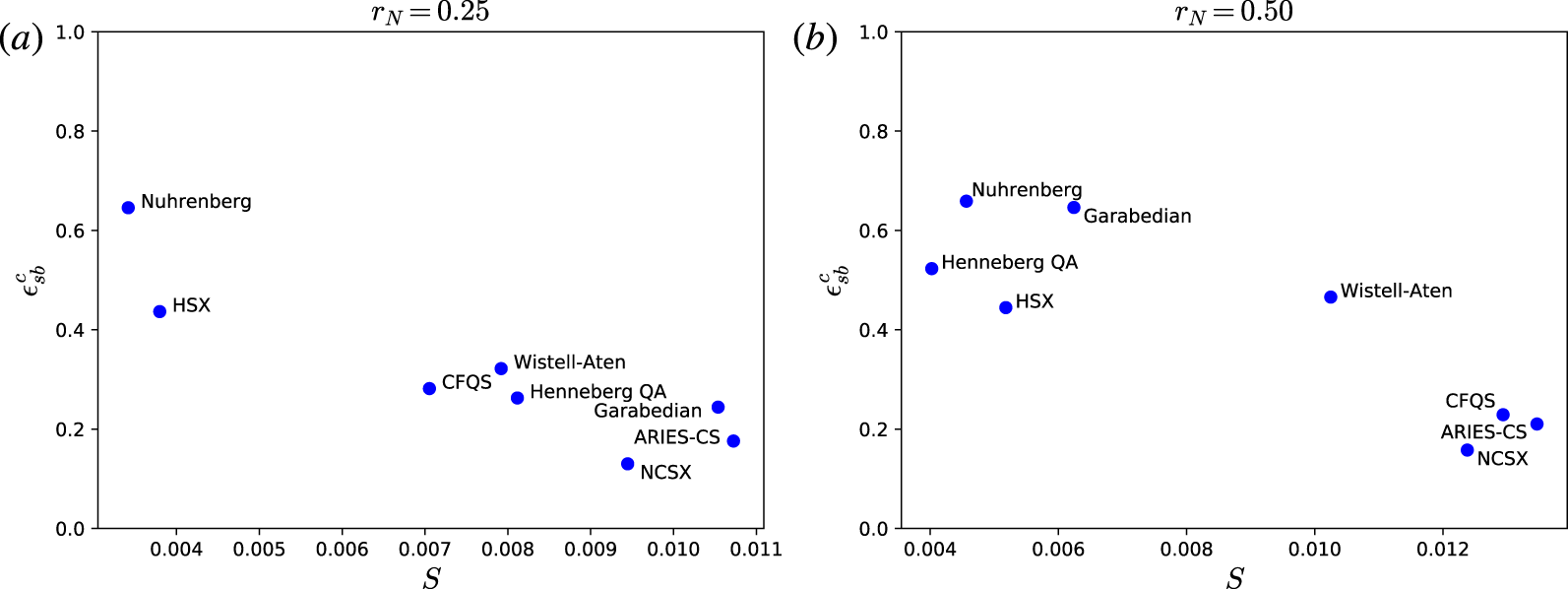
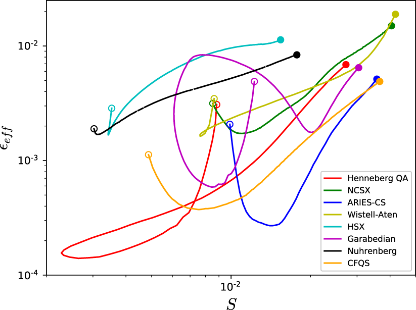
Finally, we compared the critical amount of symmetry breaking that it takes to change the sign of the particle flux,  $\unicode[STIX]{x1D716}_{sb}^{c}$, to two metrics that have been used to quantify symmetry on a flux surface. These metrics are the effective helical ripple (Nemov et al. Reference Nemov, Kasilov, Kernbichler and Heyn1999),
 $\unicode[STIX]{x1D716}_{eff}$, which is a measure of neoclassical transport in the
 $1/\unicode[STIX]{x1D708}$ regime, and the magnitude of the symmetry-breaking terms on a flux surface,
 $S$ (see (6.1)). While it was found that there was some anti-correlation between
 $\unicode[STIX]{x1D716}_{sb}^{c}$ and
 $S$, there does not appear to be much of a relationship between
 $\unicode[STIX]{x1D716}_{eff}$ and
 $\unicode[STIX]{x1D716}_{sb}^{c}$. (This should not be surprising, however, if one considers that W7-X has a very low
 $\unicode[STIX]{x1D716}_{eff}$, yet it is far from quasisymmetry.) This difference between how
 $\unicode[STIX]{x1D716}_{eff}$ and
 $S$ depend on
 $\unicode[STIX]{x1D716}_{sb}^{c}$, a quantity related to symmetry, motivates a comparison between
 $\unicode[STIX]{x1D716}_{eff}$ and
 $S$. Results indicate a configuration-specific dependence of
 $\unicode[STIX]{x1D716}_{eff}$ on
 $S$, which in many cases is non-monotonic. There is thus a disconnect between these two quantities, such that minimizing the amount of symmetry breaking on a flux surface does not simultaneously minimize
 $\unicode[STIX]{x1D716}_{eff}$. So while
 $\unicode[STIX]{x1D716}_{eff}$ is a useful proxy for optimizing neoclassical transport in stellarator optimization, it is a poor proxy for achieving good quasisymmetric surfaces.
This paper is organized as follows. In § 2.1, we introduce the governing equation and ordering assumptions of SFINCS in the results presented herein. In § 2.2, we explain the principle of ambipolarity, the fundamentals of the temperature screening phenomenon, and the issues that arise in non-axisymmetric geometries. In § 3 we explain our approach to varying the degree of quasisymmetry on a flux surface. The quasisymmetric configurations that have been explored, and the way that these equilibria have been scaled can be found in § 5. Section 4 explains an issue in present neoclassical stellarator codes based on the  $v_{E}\sim \unicode[STIX]{x1D70C}_{\ast }v_{ta}$ ordering, which limits the value of the radial electric field when impurities are included. Section 6.1 presents results on how the amount of symmetry breaking, collisionality and density gradient affect the behaviour of the impurity particle flux for various quasisymmetric configurations. Section 6.2 compares the results of § 6.1 to a gyro-Bohm estimate of turbulent particle and heat fluxes as a function of the impurity species, and normalized radius. Finally, § 7 compares the effective helical ripple to the amplitude of symmetry-breaking terms on a flux surface.
2 Background
2.1 Drift-kinetic equation
Neoclassical transport follows from a drift ordering of the Fokker–Planck equation in toroidal magnetic geometry, and solving the resulting drift-kinetic equation (equation (19) in Hazeltine (Reference Hazeltine1973)). The drift ordering assumes  $\unicode[STIX]{x1D70C}_{\ast a}=\unicode[STIX]{x1D70C}_{a}/L\ll 1$,
 $v_{E}\sim \unicode[STIX]{x1D70C}_{\ast a}v_{ta}$,
 $\unicode[STIX]{x2202}/\unicode[STIX]{x2202}t\sim \unicode[STIX]{x1D70C}_{\ast a}^{2}v_{ta}/L$, and
 $\unicode[STIX]{x1D708}_{a}\sim v_{ta}/L$, where
 $\unicode[STIX]{x1D708}_{a}$ is the collision frequency. The gyroradius of species
 $a$ is
 $\unicode[STIX]{x1D70C}_{a}=v_{ta}/\unicode[STIX]{x1D6FA}_{a}$, the thermal velocity
 $v_{ta}=\sqrt{2T_{a}/m_{a}}$, with
 $T_{a}$ and
 $m_{a}$ the temperature and mass of species
 $a$, respectively. The gyrofrequency is
 $\unicode[STIX]{x1D6FA}_{a}=Z_{a}eB/m_{a}c$, where
 $Z_{a}$ is the species charge,
 $B$ is the magnetic field magnitude,
 $c$ is the speed of light and
 $e$ is the proton charge.
Results in this paper have been obtained by solving the drift-kinetic equation (DKE) using the SFINCS (Landreman et al. Reference Landreman, Smith, Mollén and Helander2014) code over a range of collisionality regimes, for various impurity ions. SFINCS is a radially local DKE solver that has been generalized to non-axisymmetry, allowing for an arbitrary number of species, fully linearized Fokker–Planck collision operator, and the capability of simulating on-surface variations in the electrostatic potential,  $\unicode[STIX]{x1D6F7}_{1}$. The exact form of the DKE that is solved in SFINCS for this paper (with the exception of § 6.2.2) is given by equation (16) in Landreman et al. (Reference Landreman, Smith, Mollén and Helander2014)
 $$\begin{eqnarray}\dot{\boldsymbol{r}}\boldsymbol{\cdot }(\unicode[STIX]{x1D735}f_{a1})_{x_{a},\unicode[STIX]{x1D709}}+{\dot{x}}_{a}\left(\frac{\unicode[STIX]{x2202}f_{a1}}{\unicode[STIX]{x2202}x_{a}}\right)_{\boldsymbol{r},\unicode[STIX]{x1D709}}+\dot{\unicode[STIX]{x1D709}}_{a}\left(\frac{\unicode[STIX]{x2202}f_{a1}}{\unicode[STIX]{x2202}\unicode[STIX]{x1D709}}\right)_{\boldsymbol{r},x_{a}}-C_{a}=-(\boldsymbol{v}_{ma}\boldsymbol{\cdot }\unicode[STIX]{x1D735}r)\left(\frac{\unicode[STIX]{x2202}F_{a}}{\unicode[STIX]{x2202}r}\right)_{W_{a0}},\end{eqnarray}$$
where  $F_{a}$ and
 $f_{a1}$ represent a Maxwellian distribution and the first-order perturbation to the distribution function, respectively. The position vector is given by
 $\boldsymbol{r}$, the cosine of the pitch angle is
 $\unicode[STIX]{x1D709}\equiv v_{\Vert }/v$, the velocity is
 $x_{a}\equiv v/v_{ta}$,
 $W_{a0}=v^{2}/2+Z_{a}e\unicode[STIX]{x1D6F7}_{0}/m_{a}$ is the lowest-order total energy,
 $C_{a}$ is the collision operator and
 $\boldsymbol{v}_{ma}$ is the magnetic drift velocity defined by
 $$\begin{eqnarray}\boldsymbol{v}_{ma}\boldsymbol{\cdot }\unicode[STIX]{x1D735}r=\frac{m_{a}c}{Z_{a}eB^{2}}\left(v_{\Vert }^{2}+\frac{v_{\bot }^{2}}{2}\right)\boldsymbol{b}\times \unicode[STIX]{x1D735}B\boldsymbol{\cdot }\unicode[STIX]{x1D735}r.\end{eqnarray}$$
The coordinate  $r=\sqrt{2\unicode[STIX]{x1D713}_{t}/B_{av}}$ is a surface label, where
 $2\unicode[STIX]{x03C0}\unicode[STIX]{x1D713}_{t}$ is the toroidal flux, and
 $B_{av}$ is some averaged magnetic field, such as the field on the magnetic axis. The electrostatic potential is split into zeroth- and first-order contributions
 $\unicode[STIX]{x1D6F7}=\unicode[STIX]{x1D6F7}_{0}(r)+\unicode[STIX]{x1D6F7}_{1}(r,\unicode[STIX]{x1D703},\unicode[STIX]{x1D701})$, where
 $\unicode[STIX]{x1D703}$ and
 $\unicode[STIX]{x1D701}$ are the poloidal and toroidal angles. The zeroth-order term
 $\unicode[STIX]{x1D6F7}_{0}\equiv \langle \unicode[STIX]{x1D6F7}\rangle$, where
 $\langle \ldots \rangle$ is a flux-surface average, and
 $\unicode[STIX]{x1D6F7}_{1}$ is determined from the first-order quasineutrality equation
 $$\begin{eqnarray}\mathop{\sum }_{a}\left(-\frac{Z_{a}^{2}e\unicode[STIX]{x1D6F7}_{1}}{T_{a}}n_{a}+Z_{a}\int d^{3}vf_{a1}\right)=0.\end{eqnarray}$$
The time derivative terms,  $\dot{\boldsymbol{r}}$,
 ${\dot{x}}_{a}$ and
 $\dot{\unicode[STIX]{x1D709}}_{a}$ are the phase space particle trajectories. Since SFINCS offers variations in how these trajectories are defined, we have chosen to use the ‘full trajectories’ definition (equation (17) in Landreman et al. (Reference Landreman, Smith, Mollén and Helander2014)). This choice takes into account the change in potential energy as a particle drifts radially, with the corresponding change to
 $\dot{\unicode[STIX]{x1D709}}_{a}$ in order to conserve the magnetic moment,
 $\unicode[STIX]{x1D707}$. Finally, note that
 $\unicode[STIX]{x1D6F7}_{1}$ effects are neglected in these phase space trajectories and in equation § 2.1; we will discuss how
 $\unicode[STIX]{x1D6F7}_{1}$ effect can be included in § 6.2.2.
2.2 Ambipolarity and temperature screening
The property of ambipolarity can be expressed as
 $$\begin{eqnarray}\mathop{\sum }_{a}Z_{a}\unicode[STIX]{x1D6E4}_{a}=0,\end{eqnarray}$$
where  $\unicode[STIX]{x1D6E4}_{a}$ is the radial component of the particle flux of species
 $a$
 $$\begin{eqnarray}\unicode[STIX]{x1D6E4}_{a}=\left\langle \int f_{a}(\boldsymbol{v}_{ma}\boldsymbol{\cdot }\unicode[STIX]{x1D735}r)d^{3}v\right\rangle .\end{eqnarray}$$
This results from the charge density being small for length scales much longer than the Debye length. Ambipolarity is then a statement that the flux surface-averaged radial current vanishes on each flux surface. While this is true in both tokamaks and stellarators, the radial electric field is set by different physical mechanisms, and  $E_{r}$ only affects the ambipolarity condition in stellarators. The value of the radial electric field that satisfies the ambipolarity condition in a non-axisymmetric plasma is referred to as the ambipolar radial electric field.
Neoclassical fluxes are determined from a linear combination of the equilibrium gradients in the system. The radial neoclassical impurity particle flux can be written in the form of equation (1) in Velasco (Reference Velasco2017)
 $$\begin{eqnarray}\unicode[STIX]{x1D6E4}_{z}=-n_{z}\mathop{\sum }_{a}L_{11}^{a}\left[\frac{1}{n_{a}}\frac{\text{d}n_{a}}{\text{d}r}-\frac{Z_{a}eE_{r}}{T_{a}}+\unicode[STIX]{x1D6FF}_{a}\frac{1}{T_{a}}\frac{\text{d}T_{a}}{\text{d}r}\right],\end{eqnarray}$$
where  $r$ is an arbitrary radial coordinate, and
 $L_{11}^{a}$ and
 $\unicode[STIX]{x1D6FF}_{a}$ are transport coefficients (Maaßberg et al. Reference Maaßberg, Beidler and Simmet1999; Beidler Reference Beidler2011; Velasco Reference Velasco2017) that can have a complicated dependence on
 $E_{r}$ and the collision frequency
 $\unicode[STIX]{x1D708}_{z}=\unicode[STIX]{x1D708}_{zi}+\unicode[STIX]{x1D708}_{zz}$, where
 $$\begin{eqnarray}\unicode[STIX]{x1D708}_{ab}=\frac{4\sqrt{2\unicode[STIX]{x03C0}}n_{b}Z_{a}^{2}Z_{b}^{2}\ln \unicode[STIX]{x1D6EC}}{3\sqrt{m_{a}}T_{a}^{3/2}}.\end{eqnarray}$$
In the case of a tokamak, the toroidal symmetry causes the electric field dependence to cancel out in (2.4), making transport intrinsically ambipolar. This, in principle, allows for rapid toroidal rotation of the plasma, as the radial electric field profile is not governed by the ambipolarity constraint, but rather by angular momentum conservation (Shaing Reference Shaing1986; Hirshman Reference Hirshman1978; Helander & Sigmar Reference Helander and Sigmar2002; Abel et al. Reference Abel, Plunk, Wang, Barnes, Cowley, Dorland and Schekochihin2013). Moreover, for a plasma in the banana regime with  $\unicode[STIX]{x1D6FF}_{i}+\unicode[STIX]{x1D6FF}_{z}>0$, this cancellation assures a radially outward flux of the impurity species when
 $\unicode[STIX]{x1D702}_{i}^{-1}\equiv d\ln n_{i}/d\ln T_{i}<\unicode[STIX]{x1D702}_{c}^{-1}$, where
 $\unicode[STIX]{x1D702}_{c}^{-1}$ is some critical ratio of the density and temperature gradients (the ratio
 $\unicode[STIX]{x1D702}_{i}^{-1}$ is used here since
 $\unicode[STIX]{x1D735}\ln n_{i}$ drives inward impurity transport, whereas
 $\unicode[STIX]{x1D735}\ln n_{z}$ drives outward transport). This beneficial phenomenon is generally referred to as temperature screening. Specifically, we define temperature screening to be present when the flux surface-averaged impurity particle flux is positive. This definition makes clear how certain parameters affect the direction of travel of the impurities, which is ultimately the quantity of interest. However, it should be noted that temperature screening can also be defined by the sign of the temperature gradient coefficient in (2.6).
The situation is less positive in stellarator geometries since the ambipolarity condition is dependent on the radial electric field, and the temperature screening effect is no longer guaranteed. For fusion-relevant, high-density plasmas, the radial electric field is directed inward (Maaßberg et al. Reference Maaßberg, Beidler and Simmet1999) and will presumably act to drive higher- $Z$ impurities into the core. It should be stated clearly here that temperature screening is a neoclassical effect, and its presence, or lack thereof, is independent of the turbulent fluxes.
A potential solution to this situation in stellarators lies in the design of quasisymmetric configurations. A truly quasisymmetric device, whose magnetic field varies through a fixed linear combination of Boozer angles on a flux surface, will have neoclassical and guiding-centre transport properties identical to a tokamak, up to  $O(\unicode[STIX]{x1D70C}_{\ast a})$ (Pytte & Boozer Reference Pytte and Boozer1981; Boozer Reference Boozer1983). However, evidence suggests that in the absence of axisymmetry, quasisymmetry cannot be achieved exactly throughout a volume (Garren & Boozer Reference Garren and Boozer1991), meaning that quasisymmetric devices will necessarily deviate from symmetry to some level. Therefore, it would be informative to optimization efforts to know how much breaking in the symmetry of the magnetic field can be tolerated before the temperature screening effect is lost. In the following sections, we explore the effect that magnetic field symmetry breaking has on the impurity particle flux.
3 Magnetic field symmetry breaking
Any magnetic field within a flux surface can be written as a sum of harmonics in the Boozer poloidal  $\unicode[STIX]{x1D703}$, and toroidal
 $\unicode[STIX]{x1D701}$ angles (Boozer Reference Boozer1982)
 $$\begin{eqnarray}B(r,\unicode[STIX]{x1D703},\unicode[STIX]{x1D701})=\mathop{\sum }_{m,n}B_{mn}(r)\text{e}^{\text{i}(m\unicode[STIX]{x1D703}-n\unicode[STIX]{x1D701})}.\end{eqnarray}$$
Only by expressing the magnetic field in Boozer coordinates will the property of quasisymmetry become apparent. A magnetic field is considered quasisymmetric if its magnitude varies within a flux surface only through the fixed linear combination  $\unicode[STIX]{x1D712}=M\unicode[STIX]{x1D703}+N\unicode[STIX]{x1D701}$, where
 $M,N$ are fixed integers, one of which may be zero. However, since perfect quasisymmetry is not practically achievable, it is possible to express the magnetic field of a quasisymmetric configuration as a sum of quasisymmetric and non-quasisymmetric Boozer harmonics, the latter of which will be referred to as symmetry-breaking terms. Therefore, symmetry-breaking terms with smaller magnitudes will produce better approximations to perfect symmetry.
Our approach to understanding temperature screening in stellarators exploits this fact by allowing one to adjust the amplitude of the symmetry-breaking terms by an overall, constant scaling factor. The way we have decided to approach this is to expand in the harmonics of  $1/B^{2}$, which can be expressed as
 $$\begin{eqnarray}\frac{1}{B^{2}}=\mathop{\sum }_{q}h_{q}(r)\text{e}^{\text{i}q\unicode[STIX]{x1D712}}+\unicode[STIX]{x1D716}_{sb}\mathop{\sum }_{m,n}h_{mn}(r)\text{e}^{\text{i}(m\unicode[STIX]{x1D703}-n\unicode[STIX]{x1D701})},\end{eqnarray}$$
where the quantities  $h_{q}$ and
 $h_{mn}$ are the quasisymmetric and non-quasisymmetric harmonics of the
 $1/B^{2}$ expansion, respectively. The parameter
 $\unicode[STIX]{x1D716}_{sb}$ is a scaling factor (fixed for a given simulation) that controls the amplitude of the symmetry-breaking terms. The special case of
 $\unicode[STIX]{x1D716}_{sb}=0$ denotes a truly quasisymmetric field, while
 $\unicode[STIX]{x1D716}_{sb}=1$ corresponds to the original magnetic field that one would get from an equilibrium code. By running simulations with
 $\unicode[STIX]{x1D716}_{sb}$ between these values, one can gain further insight into how temperature screening is affected under magnetic fields with varying degrees of symmetry breaking.
In the context of MHD, artificially scaling the magnetic field with  $\unicode[STIX]{x1D716}_{sb}\neq 1$ will lead to a plasma that no longer satisfies the equations of an MHD equilibrium. However, if we consider the work of Garren/Boozer (Garren & Boozer Reference Garren and Boozer1991), it is likely that the construction of a single quasisymmetric flux surface is possible. Then, an arbitrarily quasisymmetric magnetic field could be constructed on one of many flux surfaces that, in principle, will satisfy an MHD equilibrium. Since this applies to only one flux surface, our approach prevents the scaling of multiple flux surfaces simultaneously.
To understand our choice of expanding  $1/B^{2}$, it is important to recognize that artificially scaling the magnetic field of an MHD equilibrium can potentially become problematic if large currents are introduced near rational surfaces (Boozer Reference Boozer1981; Helander Reference Helander2014). This can be seen in the expression for the parallel current (Helander Reference Helander2014)
 $$\begin{eqnarray}J_{\Vert }\sim \frac{h_{mn}}{r-r_{mn}}\frac{\text{d}p}{\text{d}r}.\end{eqnarray}$$
Since our simulations will always assume a finite pressure gradient, the  $h_{mn}$ modes must vanish on rational surfaces to avoid an infinite Pfirsch–Schlüter current. Therefore, scaling
 $h_{mn}$ modes as opposed to
 $B_{mn}$ modes will guarantee that such currents will not appear in this altered equilibrium.
4 Resonant radial electric field considerations
In tokamaks, it is well known that rapid plasma rotation is possible in the toroidal direction as a result of symmetry. If one then assumes the ordering of  $v_{E}\sim v_{ta}$, then radial electric fields are capable of producing sonic flows. The radial electric field that corresponds to sonic rotation is known as the resonant electric field, which in axisymmetry is
 $E_{r}^{res}=r\unicode[STIX]{x1D704}Bv_{ta}/(Rc)$ (Beidler Reference Beidler2008). We take the radial electric field here to be defined by
 $E_{r}\equiv -\text{d}\unicode[STIX]{x1D6F7}/\text{d}r$.
Constraints on the symmetry of the magnetic field, however, prevent ordering the flow velocity with the thermal speed in generic stellarators (Helander Reference Helander2007), as well as perfectly quasisymmetry ones (Sugama et al. Reference Sugama, Watanabe, Nunami and Nishimura2011a). The form of the drift-kinetic equation that is solved in SFINCS uses the  $v_{E}\sim \unicode[STIX]{x1D70C}_{\ast a}v_{ta}$ ordering to avoid the symmetric restrictions to the magnetic field that result from sonic flows. From the SFINCS ordering, the vast majority of parameter regimes, geometries and species, yield ambipolar radial electric fields,
 $E_{r}^{a}$, that are considerably smaller than the resonant electric field magnitude. However, the
 $m_{a}^{-1/2}$ dependence of the resonant electric field can cause the ordering to break down for heavy impurities under certain conditions. Solving this issue completely would demand a reordering to derive a new form of the drift-kinetic equation. We do not attempt to tackle this problem here, but leave it to future work.
It is also very interesting and relevant to note that QH configurations produce a considerably larger gap between  $E_{r}^{a}$ and
 $E_{r}^{res}$ than QA configurations for otherwise identical plasma parameters. The relative size of these electric fields for a given simulation can be found by deriving an analogous expression for the resonant radial electric field in quasisymmetry.
If we start by assuming the  $v_{E}\sim v_{ta}$ ordering, then the
 $v_{E}$ and parallel streaming terms will be of the same order
 $$\begin{eqnarray}v_{\Vert }\hat{\boldsymbol{b}}\boldsymbol{\cdot }\unicode[STIX]{x1D735}\unicode[STIX]{x1D712}\sim \frac{c}{B^{2}}\boldsymbol{E}\times \boldsymbol{B}\boldsymbol{\cdot }\unicode[STIX]{x1D735}\unicode[STIX]{x1D712},\end{eqnarray}$$
where  $\unicode[STIX]{x1D712}=M\unicode[STIX]{x1D703}-N\unicode[STIX]{x1D701}$. The contravariant and covariant representations of the magnetic field are, respectively,
 $$\begin{eqnarray}\displaystyle & \displaystyle \boldsymbol{B}=\unicode[STIX]{x1D735}\unicode[STIX]{x1D713}_{t}\times \unicode[STIX]{x1D735}\unicode[STIX]{x1D703}+\unicode[STIX]{x1D704}\unicode[STIX]{x1D735}\unicode[STIX]{x1D701}\times \unicode[STIX]{x1D735}\unicode[STIX]{x1D713}_{t} & \displaystyle\end{eqnarray}$$
 $$\begin{eqnarray}\displaystyle & \displaystyle \boldsymbol{B}=L\unicode[STIX]{x1D735}\unicode[STIX]{x1D713}_{t}+I\unicode[STIX]{x1D735}\unicode[STIX]{x1D703}+G\unicode[STIX]{x1D735}\unicode[STIX]{x1D701}, & \displaystyle\end{eqnarray}$$
where  $2\unicode[STIX]{x03C0}\unicode[STIX]{x1D713}_{t}$ is the toroidal flux,
 $L=L(\unicode[STIX]{x1D713}_{t},\unicode[STIX]{x1D703},\unicode[STIX]{x1D701})$ is some scalar, and as detailed in Helander (Reference Helander2014)
 $$\begin{eqnarray}\displaystyle & \displaystyle \int _{S_{\unicode[STIX]{x1D701}}}\boldsymbol{J}\boldsymbol{\cdot }\unicode[STIX]{x1D735}\unicode[STIX]{x1D701}\sqrt{g}\,\text{d}\unicode[STIX]{x1D703}\,\text{d}\unicode[STIX]{x1D713}_{t}=\frac{c}{2}I(\unicode[STIX]{x1D713}_{t}) & \displaystyle\end{eqnarray}$$
 $$\begin{eqnarray}\displaystyle & \displaystyle \int _{S_{\unicode[STIX]{x1D703}}}\boldsymbol{J}\boldsymbol{\cdot }\unicode[STIX]{x1D735}\unicode[STIX]{x1D703}\sqrt{g}\,\text{d}\unicode[STIX]{x1D701}\,\text{d}\unicode[STIX]{x1D713}_{t}=\frac{c}{2}G(\unicode[STIX]{x1D713}_{t}), & \displaystyle\end{eqnarray}$$
where  $1/\sqrt{g}=(\unicode[STIX]{x1D735}\unicode[STIX]{x1D713}_{t}\times \unicode[STIX]{x1D735}\unicode[STIX]{x1D703})\boldsymbol{\cdot }\unicode[STIX]{x1D735}\unicode[STIX]{x1D701}$ is the Jacobian, and
 $S_{\unicode[STIX]{x1D701}}$ and
 $S_{\unicode[STIX]{x1D703}}$ correspond to surfaces where
 $\unicode[STIX]{x1D701}=\text{const}.$ and
 $\unicode[STIX]{x1D703}=\text{const}.$, respectively. Solving for
 $E_{r}$ when
 $v_{E}\sim v_{\Vert }\sim v_{th}$ yields an expression for the resonant electric field
 $$\begin{eqnarray}E_{r}^{res}\sim \left|\frac{rv_{ta}B^{2}}{c}\frac{M\unicode[STIX]{x1D704}-N}{MG+NI}\right|.\end{eqnarray}$$
Typically,  $I\ll G$, so the QH devices examined in the following sections (all of which have
 $M=1$,
 $|N|\geqslant 4$) will have
 $(E_{r}^{res})_{QH}\simeq |(\unicode[STIX]{x1D704}-N)/\unicode[STIX]{x1D704}|(E_{r}^{res})_{QA}$. This allows one to run neoclassical codes at larger
 $E_{r}^{a}$ before the ordering breakdown is reached. For this reason, only QH results are available in some SFINCS simulations with steep gradients and/or heavier impurity ions. As a workaround for QA, we have only considered cases where
 $E_{r}^{a}/E_{r}^{res}<1/3$, in order to be sufficiently far from the resonance to avoid unreliable results due to the breakdown of
 $v_{E}\sim \unicode[STIX]{x1D70C}_{\ast a}v_{ta}$.
5 Magnetic field configurations
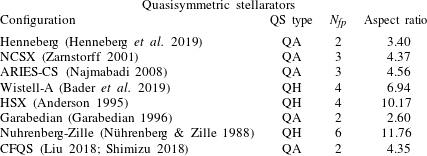
Throughout the remainder of this paper, we aim to provide results that are general to a wide range of quasisymmetric stellarators. We have therefore chosen 8 distinct quasisymmetric stellarator configurations (summarized in table 1) to examine, some of which were designed to be QA, and the others QH. Here, we have used the C09R00 equilibrium from NCSX, the Nuhrenberg configuration from figure 1 and table 1 in Nührenberg & Zille (Reference Nührenberg and Zille1988), and the (QH) configuration of HSX. HSX is the only configuration in this list that has been constructed to date. To allow for a fair comparison between devices, each device was scaled to the minor radius,  $a$, and on-axis magnetic field,
 $B_{0}$, of the Henneberg et al. QA configuration (Henneberg et al. Reference Henneberg, Drevlak, Nührenberg, Beidler, Turkin, Loizu and Helander2019),
 $a=0.602~\text{m}$ and
 $B_{0}=2.10~\text{T}$.
Quasisymmetric stellarator configurations that have been studied in this work.  $N_{fp}$: number of field periods.

6 Results
The results generated below employ the full linearized Fokker–Planck collision operator of SFINCS, with two ion species. The main ions are taken to be hydrogen in each of the simulations, while the charge and mass of the impurity ion can vary between runs. Unless otherwise specified (6.2.2), the electrostatic potential is taken to be constant on a flux surface  $\unicode[STIX]{x1D6F7}=\unicode[STIX]{x1D6F7}_{0}(r)$. It is assumed here that ion temperatures are equivalent,
 $T_{i}=T_{z}$, due to the fast equilibration time. The choice of the temperature and density profiles in the following results is based on the modelling of an ECRH-heated, W7-X plasma in figure 5 of Turkin et al. (Reference Turkin, Beidler, Maaßberg, Murakami, Tribaldos and Wakasa2011). The density gradient, however, is not determined from figure 5 in Turkin et al. (Reference Turkin, Beidler, Maaßberg, Murakami, Tribaldos and Wakasa2011), but rather chosen so as to give particular values of
 $\unicode[STIX]{x1D702}^{-1}$. Further, the density gradient is taken to be equivalent between ion species
 $\unicode[STIX]{x1D735}\ln n_{i}=\unicode[STIX]{x1D735}\ln n_{z}$ (or equivalently
 $\unicode[STIX]{x1D702}^{-1}=\unicode[STIX]{x1D702}_{i}^{-1}=\unicode[STIX]{x1D702}_{z}^{-1}$), meaning that the profile of
 $Z_{eff}$ is flat.
The recent work of Helander et al. (Reference Helander, Newton, Mollén and Smith2017) has shown that temperature screening can be achieved in reactor-relevant, mixed-collisionality plasmas (highly collisional impurities and low-collisionality bulk ions) at large normalized radius  $r_{N}=0.88$. With the increased temperature in the core, however, it is possible that the bulk ions and impurities in reactor-grade plasmas will both have low collisionalities, depending of course on the particular impurity ion. The picture for temperature screening becomes more pessimistic as collisionality decreases, which can be seen in figures 1 and 2 in Helander et al. (Reference Helander, Newton, Mollén and Smith2017). For our purposes of understanding how much symmetry breaking can be tolerated prior to losing this effect, we choose to study collisionalities below the region of temperature screening in Helander et al. (Reference Helander, Newton, Mollén and Smith2017), in order to ensure that this transition will be observed in at least some cases.
Specifically, in the results that follow, both the ions and impurities will fall into what is generally considered the low-collisionality regime in stellarators  $\unicode[STIX]{x1D708}_{\ast }^{a}\ll 1$, where we define
 $\unicode[STIX]{x1D708}_{\ast }^{a}\equiv \unicode[STIX]{x1D708}_{a}R/v_{ta}$. The low-collisionality regime can be further subdivided into the plateau,
 $1/\unicode[STIX]{x1D708}$, and
 $\sqrt{\unicode[STIX]{x1D708}}$ regimes, as derived for realistic aspect ratio in Calvo et al. (Reference Calvo, Parra, Velasco, Alonso and García-Regaña2018). The plateau regime is defined by
 $\unicode[STIX]{x1D716}^{3/2}\ll \unicode[STIX]{x1D708}_{\ast }^{a}\ll 1$, the
 $1/\unicode[STIX]{x1D708}$ regime by
 $\unicode[STIX]{x1D716}^{-1}\unicode[STIX]{x1D70C}_{\ast a}\ll \unicode[STIX]{x1D708}_{\ast }^{a}\ll \unicode[STIX]{x1D716}^{3/2}$ and the
 $\sqrt{\unicode[STIX]{x1D708}}$ regime by
 $\unicode[STIX]{x1D708}_{\ast }^{a}\ll \unicode[STIX]{x1D716}^{-1}\unicode[STIX]{x1D70C}_{\ast a}$, where
 $\unicode[STIX]{x1D716}\equiv a/R$. We further explicitly define the equilibrium length scale in
 $\unicode[STIX]{x1D70C}_{\ast a}\equiv \unicode[STIX]{x1D70C}_{a}/R$ to be consistent with the use of the major radius in the definitions of Calvo et al. (Reference Calvo, Parra, Velasco, Alonso and García-Regaña2018).
6.1 Impact of magnetic field symmetry breaking on impurity particle flux
6.1.1 Flat density profile:  $\unicode[STIX]{x1D702}^{-1}=0$

As one increases the magnitude of  $\unicode[STIX]{x1D716}_{sb}$ from 0 up to the true magnetic field, the transport due to the helical wells will also increase. It is not clear a priori exactly how this incremental breaking of symmetry will change the impurity particle flux. However, it is clear that for many cases of interest there should be some critical value,
 $\unicode[STIX]{x1D716}_{sb}^{c}$, where the radial impurity particle flux,
 $\unicode[STIX]{x1D6E4}_{z}$, changes sign, which will depend on the particular magnetic equilibrium.
In this section, we examine the  $\unicode[STIX]{x1D716}_{sb}$ dependence of
 $\unicode[STIX]{x1D6E4}_{z}$ for each of the configurations in table 1 in select parameter regimes. It should be understood that the magnitude of
 $\unicode[STIX]{x1D6E4}_{z}$ is less important than the sign in this section.
The  $E_{r}$ for each simulation was chosen to be the ambipolar
 $E_{r}$ for the
 $\unicode[STIX]{x1D716}_{sb}=1$ case, considering that
 $E_{r}$ becomes progressively less important in calculating radial fluxes as the magnetic field approaches symmetry (this can be seen from figure 6, which is discussed at the end of this section). It also becomes difficult to accurately calculate the radial electric field for small values of
 $\unicode[STIX]{x1D716}_{sb}$. We choose fully ionized carbon,
 $\text{C}^{6+}$, as the impurity in figures 1 and 3 in order to avoid proximity to the resonant electric field in all configurations (see § 4). Finally, we take
 $\unicode[STIX]{x1D6FC}=\sum _{a\neq i}n_{a}Z_{a}^{2}/(n_{i}Z_{i}^{2})=1$, corresponding to
 $Z_{eff}=2$.
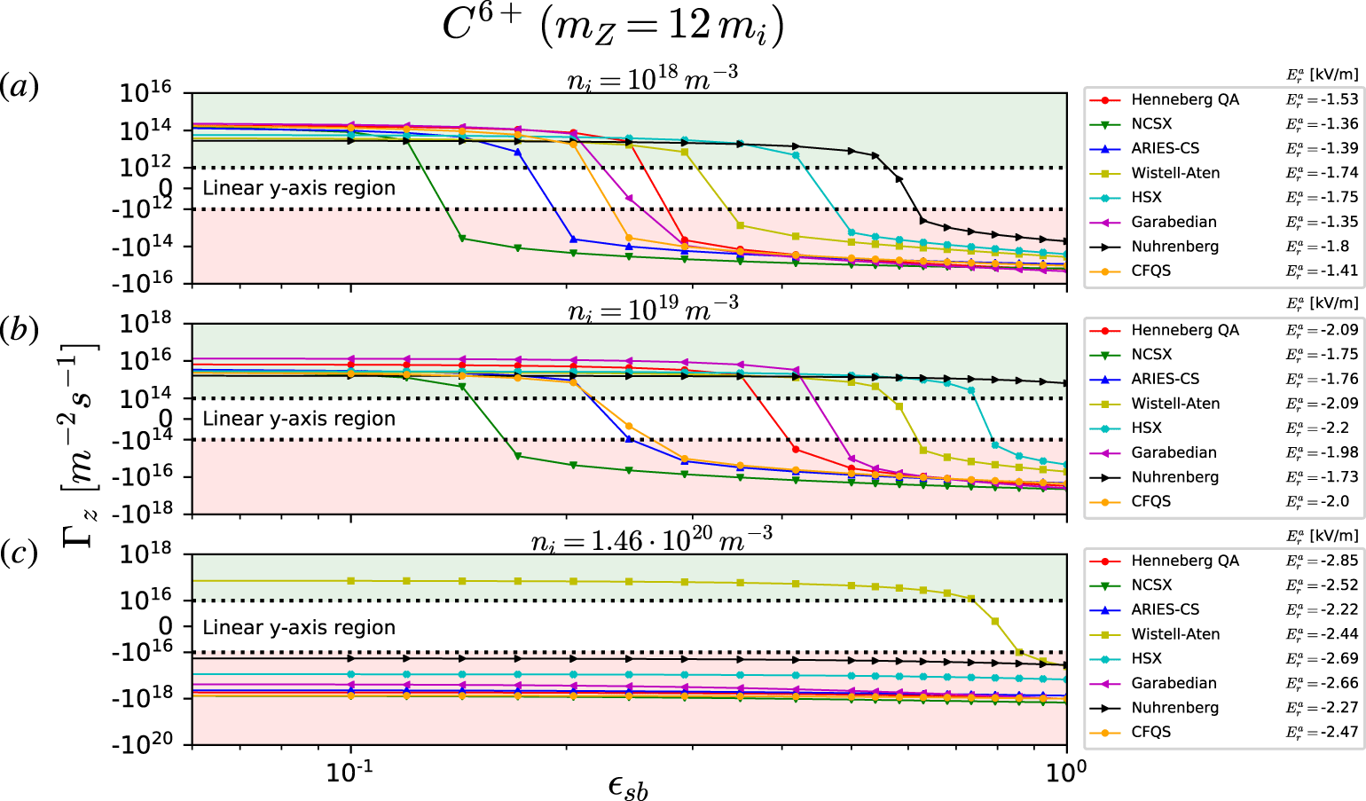
The impurity particle flux at  $\unicode[STIX]{x1D702}^{-1}=0$ for
 $\text{C}^{6+}$ is plotted as a function of the symmetry-breaking amplitude at a normalized radius of
 $r_{N}=0.25$.
 $T=4~\text{keV}$,
 $\text{d}T/\text{d}r=-0.97~\text{keV}~\text{m}^{-1}$ and
 $Z_{eff}=2$ were kept constant for all panels. The upper, green-shaded region denotes positive
 $\unicode[STIX]{x1D6E4}_{z}$ (impurity screening). The lower, red-shaded region corresponds to negative
 $\unicode[STIX]{x1D6E4}_{z}$ (impurity accumulation). The normalized
 $\text{C}^{6+}$ gyroradius is
 $\unicode[STIX]{x1D70C}_{\ast z}=4.17\times 10^{-3}\;\unicode[STIX]{x1D716}$, and the collisionalities for each panel are (a)
 $\unicode[STIX]{x1D708}_{\ast }^{z}=2.26\times 10^{-4}\;\unicode[STIX]{x1D716}^{-1}$, (b)
 $\unicode[STIX]{x1D708}_{\ast }^{z}=2.26\times 10^{-3}\;\unicode[STIX]{x1D716}^{-1}$ and (c)
 $\unicode[STIX]{x1D708}_{\ast }^{z}=3.29\times 10^{-2}\;\unicode[STIX]{x1D716}^{-1}$.

In figure 1(a–c), we have plotted results at  $r_{N}\simeq 0.25$ for all devices at increasing values of collisionality, which is achieved by varying the ion density at constant temperature. Here, and in the results that follow,
 $r_{N}\equiv r/a=\sqrt{\unicode[STIX]{x1D713}_{t}/\unicode[STIX]{x1D713}_{a}}$, where
 $a$ is the minor radius, and
 $2\unicode[STIX]{x03C0}\unicode[STIX]{x1D713}_{a}$ is the toroidal flux at the last closed flux surface (computed in VMEC (Hirshman, van Rij & Merkel Reference Hirshman, van Rij and Merkel1986b)). At this radial location we take
 $T_{i}=T_{z}=4~\text{keV}$ and
 $\text{d}T_{i}/\text{d}r=\text{d}T_{z}/\text{d}r=-0.97~\text{keV}~\text{m}^{-1}$. In the lowest-collisionality case of figure 1(a) (with
 $n_{i}=10^{18}~\text{m}^{-3}$), there is a similar
 $\unicode[STIX]{x1D716}_{sb}$ dependence of
 $\unicode[STIX]{x1D6E4}_{z}$ for each of the devices, regardless of the type of quasisymmetry (QA or QH). For a magnetic field with near-perfect quasisymmetry (
 $\unicode[STIX]{x1D716}_{sb}=10^{-2}$), the resulting
 $\unicode[STIX]{x1D6E4}_{z}$ is positive, indicating a presence of the temperature screening effect. As
 $\unicode[STIX]{x1D716}_{sb}$ is increased,
 $\unicode[STIX]{x1D6E4}_{z}$ decreases until eventually changing sign at some value of
 $\unicode[STIX]{x1D716}_{sb}<1$.
The first thing that can be understood from this plot is that at this collisionality, none of the devices that were studied displayed temperature screening at the actual magnetic field,  $\unicode[STIX]{x1D716}_{sb}=1$. However, the value of
 $\unicode[STIX]{x1D716}_{sb}^{c}$ where temperature screening is lost will depend on the magnetic configuration. In the case of Nuhrenberg-Zille, for example, the transition occurs at
 $\unicode[STIX]{x1D716}_{sb}^{c}\simeq 0.6$, which is essentially saying that the symmetry-breaking terms must be
 ${\sim}60\,\%$ of their actual values to ensure temperature screening under these conditions. Toward the left side of the plot, the NCSX transition occurs at
 $\unicode[STIX]{x1D716}_{sb}^{c}\simeq 0.1$, requiring the symmetry-breaking terms to be
 ${\sim}10\times$ smaller.
In figure 1(b), the same plot as in figure 1(a) is constructed, however, the density (and hence collisionality) has been increased by an order of magnitude. First, it should be remarked that at this collisionality, the Nuhrenberg–Zille configuration actually achieves temperature screening at  $\unicode[STIX]{x1D716}_{sb}=1$. While this is the only such configuration to do so, it is also true that
 $\unicode[STIX]{x1D716}_{sb}^{c}$ has increased for each configuration from the respective values in figure 1(a). Since
 $\unicode[STIX]{x1D716}_{sb}^{c}$ can approximate closeness to quasisymmetry, it follows that increasing the collisionality appears to improve the ‘effective quasisymmetry’ of a flux surface, as it relates to impurity transport.
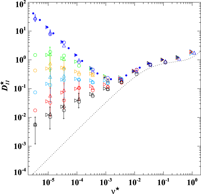
The meaning behind our use of the term ‘effective quasisymmetry’, which is only applicable for impurity transport and not bulk particles, can nevertheless be understood from a figure in Beidler (Reference Beidler2011) looking at bulk ion transport (which has been reused in figure 2 with permissions). For comparison, the normalized ion collisionality of figure 1(a) corresponds to  $\unicode[STIX]{x1D708}^{\ast }\sim 10^{-5}$ in figure 2. At low collisionality, there is a difference (depending on
 $E_{r}$) between the
 $D_{11}$ coefficient (describing radial transport) for HSX and the perfectly quasisymmetric case, indicating a sensitivity of the particles to the exact structure of the magnetic field. As collisionality is increased, this difference becomes less pronounced as the contribution to transport from helically trapped particles decreases. At a high enough collisionality,
 $D_{11}$ in figure 2 is about the same for perfect quasisymmetry as it is for HSX, regardless of
 $E_{r}$. Noting that the magnetic trapping structures can be quite different in perfect symmetry and a nominally quasisymmetric field, the similarities in
 $D_{11}$ indicate a decreased sensitivity of the particles to the exact structure of the magnetic field at higher collisionalities. Thus, in the context of quasisymmetry, increasing the collisionality brings the transport closer to symmetric levels, ‘effectively’ increasing quasisymmetry.
Definitions of normalizations, markers/colours, and details can be found in figure (14) of Beidler (Reference Beidler2011). The  $D_{11}$ transport coefficient is plotted as a function of collisionality for HSX geometry. Here, the colours represent different
 $v_{E}$ values. DKES (Hirshman et al. Reference Hirshman, Shaing, van Rij, Beasley and Crume1986a; van Rij & Hirshman Reference van Rij and Hirshman1989) results are depicted by triangles (▵), NEO-2 (Nemov et al. Reference Nemov, Kasilov, Kernbichler and Heyn1999; Kernbichler et al. Reference Kernbichler, Kasilov, Leitold, Nemov and Allmaier2008) by filled circles (●) and Monte Carlo results are plotted using open circles (○) (Tribaldos Reference Tribaldos2001), and right-point triangles (▹) (Allmaier et al. Reference Allmaier, Kasilov, Kernbichler and Leitold2008). The dotted line is a simulation with equivalent perfect helical symmetry and
 $E_{r}=0$.

However, there is a limit to the beneficial impacts of increasing the density, as can be seen in figure 1(c), where  $n_{i}=1.46\times 10^{20}~\text{m}^{-3}$. Aside from the Wistell-A configuration, all of the other configurations at near-perfect quasisymmetry do not display an outward impurity flux. There are two possible explanations for why this might take place in perfect symmetry. First, for QA configurations, it is possible that
 $E_{r}^{a}$ and
 $E_{r}^{res}$ are close enough that ambipolarity no longer holds, and the higher-order
 $E_{r}$ terms (Sugama et al. Reference Sugama, Watanabe, Nunami and Nishimura2011b) become important. To explain this effect in QH, one must recall that temperature screening in axisymmetry is not predicted at high collisionalities (Rutherford Reference Rutherford1974), except for cases where
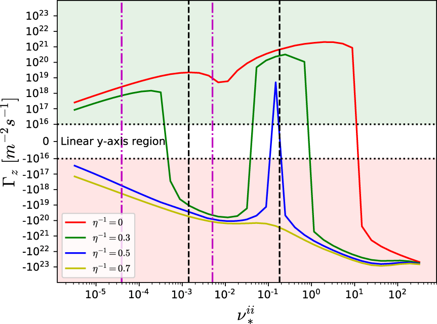
 $\unicode[STIX]{x1D6FC}\rightarrow 0$ for collisional ions and impurities. In appendix A, it can be seen that beyond some critical
 $\unicode[STIX]{x1D708}_{\ast }^{ii}$ in axisymmetry, the impurity flux becomes negative for most
 $\unicode[STIX]{x1D702}^{-1}$. Figure 1(c) is thus indicating that we are hovering around that critical collisionality where temperature screening is not possible, even in perfect symmetry. It is interesting to note here that in figure 1(a,b), the impurities are mostly in the
 $\sqrt{\unicode[STIX]{x1D708}}$ or
 $1/\unicode[STIX]{x1D708}$ regime. However, in figure 1(c), all QH configurations are well into the plateau regime, and most of the QA configurations have transitioned to the plateau regime as well. The ions are in the
 $\sqrt{\unicode[STIX]{x1D708}}$ regime in all but a couple cases at the highest collisionality.
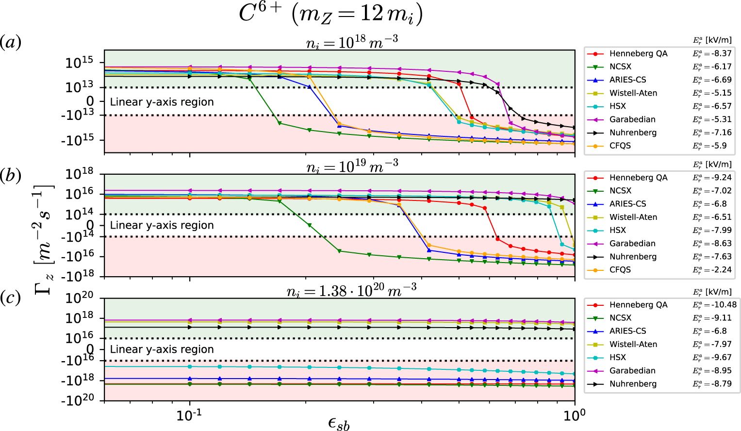
The situation is less pessimistic in figure 3, where we look at  $r_{N}=0.50$ with
 $T=3.3~\text{keV}$ and
 $\text{d}T/\text{d}r=-4.78~\text{keV}~\text{m}^{-1}$. The trends are largely similar to figure 1 at each collisionality, however, there are a handful of cases where temperature screening can be seen at
 $\unicode[STIX]{x1D716}_{sb}=1$. Furthermore, at the highest collisionality, the Wistell-A, Garabedian and Nuhrenberg configurations have an outward impurity particle flux for all
 $\unicode[STIX]{x1D716}_{sb}$. The collisionality at
 $r_{N}=0.50$ is only slightly higher than at
 $r_{N}=0.25$, and
 $\unicode[STIX]{x1D702}^{-1}=0$ at both
 $r_{N}$, so the differences at these radii are likely caused by the distinct magnetic field modes,
 $B_{mn}$.
The impurity particle flux at  $\unicode[STIX]{x1D702}^{-1}=0$ for
 $\text{C}^{6+}$ is plotted as a function of the symmetry-breaking amplitude at a normalized radius of
 $r_{N}=0.50$.
 $T=3.3~\text{keV}$,
 $\text{d}T/\text{d}r=-4.78~\text{keV}~\text{m}^{-1}$ and
 $Z_{eff}=2$ were kept constant for all panels. The upper, green-shaded region denotes positive
 $\unicode[STIX]{x1D6E4}_{z}$ (impurity screening). The lower, red-shaded region corresponds to negative
 $\unicode[STIX]{x1D6E4}_{z}$ (impurity accumulation). The normalized
 $\text{C}^{6+}$ gyroradius is
 $\unicode[STIX]{x1D70C}_{\ast z}=3.79\times 10^{-3}\;\unicode[STIX]{x1D716}$, and the collisionalities for each panel are (a)
 $\unicode[STIX]{x1D708}_{\ast }^{z}=3.32\times 10^{-4}\;\unicode[STIX]{x1D716}^{-1}$, (b)
 $\unicode[STIX]{x1D708}_{\ast }^{z}=3.32\times 10^{-3}\;\unicode[STIX]{x1D716}^{-1}$ and (c)
 $\unicode[STIX]{x1D708}_{\ast }^{z}=4.58\times 10^{-2}\;\unicode[STIX]{x1D716}^{-1}$.

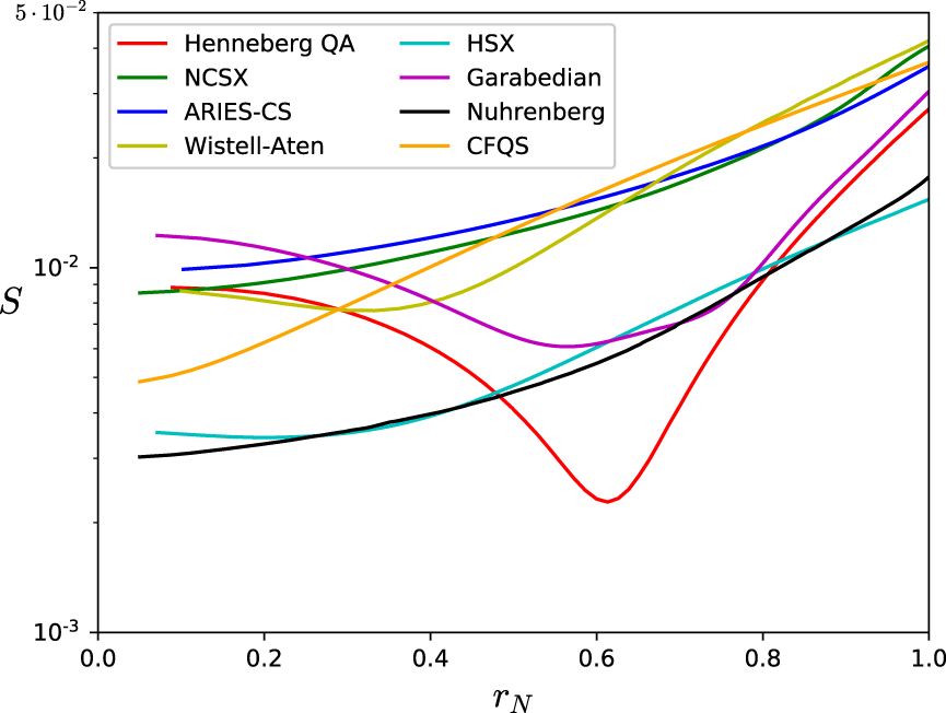
The differences between figures 1 and 3 can be understood by looking at the magnitude of symmetry-breaking terms
 $$\begin{eqnarray}S\equiv \sqrt{\mathop{\sum }_{m,n\neq mN}B_{mn}^{2}/B_{00}^{2}},\end{eqnarray}$$
as a function of  $r_{N}$ in figure 4. The summation in (6.1) includes all modes that are not an integer multiple of the dominant magnetic helicity
 $\unicode[STIX]{x1D712}$ (i.e.
 $M=1$,
 $N=4$ for HSX). If we consider the curves for Henneberg QA and Garabedian, we can compare the difference in the values of
 $\unicode[STIX]{x1D716}_{sb}^{c}$ in figures 1(a) and 3(a). In moving from
 $r_{N}=0.25$ to
 $r_{N}=0.50$ in figure 4, the symmetry-breaking amplitude for Henneberg QA and Garabedian decreases by
 ${\sim}4$. The corresponding increase in
 $\unicode[STIX]{x1D716}_{sb}^{c}$ from
 $r_{N}=0.25$ to
 $r_{N}=0.50$ is
 ${\sim}2{-}3$ for both configurations. If we were to then consider the respective CFQS curves (figures 1a and 3a), there is an increase in
 $S$ between these radii of
 ${\sim}2$, where a decrease in
 $\unicode[STIX]{x1D716}_{sb}^{c}$ is observed. This presents a connection between the closeness to quasisymmetry of a flux surface, and the realization of temperature screening. The remaining configurations have a difference in
 $S$ of less than a factor of 2 at these radii, and
 $S$ is also larger at
 $r_{N}=0.50$. Unlike the connection between
 $S$ and the change in
 $\unicode[STIX]{x1D716}_{sb}^{c}$ for Henneberg QA, Garabedian, and CFQS, the change in
 $\unicode[STIX]{x1D716}_{sb}$ is positive (although small) for the remaining configurations. This could potentially be accounted for by a complicated dependency on collisionality,
 $E_{r}$, and the aspect ratio.
The amplitude of the symmetry-breaking terms,  $S$, are plotted as a function of normalized radius,
 $r_{N}$.

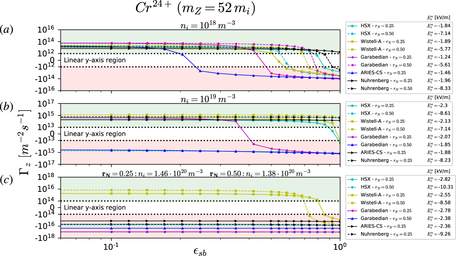
The arguments in this section are also relevant when considering higher-Z impurities. In figure 5, a similar plot to figures 1 and 3 has been constructed for  $\text{Cr}^{24+}$, where results from both
 $r_{N}=0.25$ and
 $r_{N}=0.50$ have been consolidated into figure 5. To restate from § 4, only configurations where
 $E_{r}^{a}/E_{r}^{res}<1/3$ have been considered. One difference between
 $\text{Cr}^{24+}$ and
 $\text{C}^{6+}$ is that the value of
 $\unicode[STIX]{x1D716}_{sb}^{c}$ decreases for the QA configurations between figures 5(a) and 5(b). This behaviour is likely due to the increase in collisionality from figures 1 and 3, (where the impurities are now in the plateau regime in figure 5(b) and collisional in 5c), meaning that the critical density where temperature screening is lost has decreased. Further, the behaviour of Wistell-A in figure 5 is interesting compared to other configurations. From figure 4, the values of
 $S$ at
 $r_{N}=0.25$ and
 $r_{N}=0.50$ are quite similar, however, there is clear increase in
 $\unicode[STIX]{x1D716}_{sb}^{c}$ that may not be related to the amplitude of symmetry-breaking terms.
The impurity particle flux at  $\unicode[STIX]{x1D702}^{-1}=0$ for
 $\text{Cr}^{24+}\,(m_{z}=52\,m_{i})$ is plotted as a function of the symmetry-breaking amplitude. For
 $\boldsymbol{r}_{\boldsymbol{N}}=0.25$:
 $T=4.0~\text{keV}$,
 $\text{d}T/\text{d}r=-0.97~\text{keV}~\text{m}^{-1}$ and
 $\unicode[STIX]{x1D70C}_{\ast z}=2.17\times 10^{-3}\;\unicode[STIX]{x1D716}$ with collisionalities (a)
 $\unicode[STIX]{x1D708}_{\ast }^{z}=3.61\times 10^{-3}\;\unicode[STIX]{x1D716}^{-1}$, (b)
 $\unicode[STIX]{x1D708}_{\ast }^{z}=3.61\times 10^{-2}\;\unicode[STIX]{x1D716}^{-1}$ and (c)
 $\unicode[STIX]{x1D708}_{\ast }^{z}=0.53\;\unicode[STIX]{x1D716}^{-1}$. At
 $\boldsymbol{r}_{\boldsymbol{N}}=0.50$:
 $T=3.3~\text{keV}$,
 $\text{d}T/\text{d}r=-4.78~\text{keV}~\text{m}^{-1}$ and
 $\unicode[STIX]{x1D70C}_{\ast z}=1.97\times 10^{-3}\;\unicode[STIX]{x1D716}$ with collisionalities (a)
 $\unicode[STIX]{x1D708}_{\ast }^{z}=5.31\times 10^{-3}\;\unicode[STIX]{x1D716}^{-1}$, (b)
 $\unicode[STIX]{x1D708}_{\ast }^{z}=5.31\times 10^{-2}\;\unicode[STIX]{x1D716}^{-1}$ and (c)
 $\unicode[STIX]{x1D708}_{\ast }^{z}=0.73\;\unicode[STIX]{x1D716}^{-1}$.
 $Z_{eff}=2$ was kept constant for all panels. The upper, green-shaded region denotes positive
 $\unicode[STIX]{x1D6E4}_{z}$ (impurity screening). The lower, red-shaded region corresponds to negative
 $\unicode[STIX]{x1D6E4}_{z}$ (impurity accumulation).

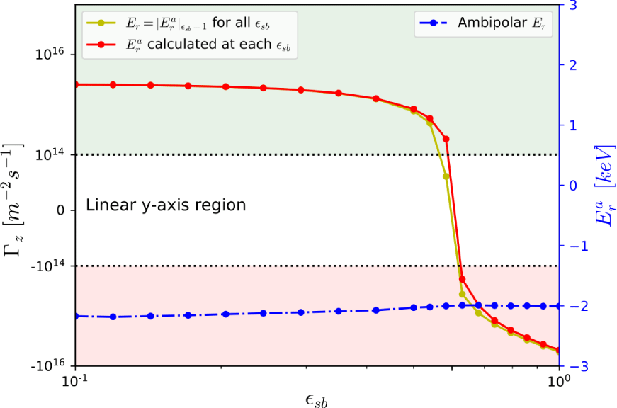
As mentioned at the beginning of this section,  $E_{r}^{a}$ at
 $\unicode[STIX]{x1D716}_{sb}=1$ has been used as the
 $E_{r}$ value for all
 $\unicode[STIX]{x1D716}_{sb}$ simulations. In figure 6, we use the Wistell-A curve from figure 1(b) and compare it to one generated with
 $E_{r}^{a}$ calculated at each
 $\unicode[STIX]{x1D716}_{sb}$, as evidence for our argument in making this approximation. From the dashed blue curve indicating the calculated
 $E_{r}^{a}$ value, there is little variation as
 $\unicode[STIX]{x1D716}_{sb}$ decreases. More importantly, this variation also has a minor impact on
 $\unicode[STIX]{x1D6E4}_{z}$, as evinced by the red curve in figure 6, which utilizes the
 $E_{r}$ values from the dashed blue curve at each
 $\unicode[STIX]{x1D716}_{sb}$.
Left  $y$-axis: the impurity particle flux is plotted as a function of the symmetry-breaking amplitude in Wistell-A using the parameters of figure 1(b). The yellow curve is identical to the yellow curve of figure 1(b). The red curve uses the calculated
 $E_{r}^{a}$ value for each
 $\unicode[STIX]{x1D716}_{sb}$. Right
 $y$-axis: the blue dashed line is the
 $E_{r}^{a}$ for each point in the red curve.

The overall results in figures 1, 3, and 5 indicate that for reactor-relevant plasma parameters, temperature screening could be achievable in certain configurations. However, as it is unlikely that the density profile will be completely flat, it is imperative to understand how  $\unicode[STIX]{x1D6E4}_{z}$ varies with
 $\unicode[STIX]{x1D702}^{-1}$.
6.1.2 Finite peaked density gradients: $\unicode[STIX]{x1D702}^{-1}>0$

Peaking of the main ion’s density profile drives an inward neoclassical impurity flux. This result is shown for axisymmetry or quasisymmetry in appendix A. In non-symmetric stellarators, the situation is complicated by not only the presence of the radial electric field as a driving gradient in the impurity flux, but the fact that  $L_{11}$ depends on
 $E_{r}$, and in different ways depending on the collisionality regime. An exact analytic solution for
 $\unicode[STIX]{x1D6E4}_{z}$ is therefore intractable in most cases. However, it is possible to approximate the solution by using a similar procedure to that used in Velasco (Reference Velasco2017), but generalizing for arbitrary
 $Z_{eff}$. We start with an expression for the particle flux of an arbitrary species that is valid far from quasisymmetry at low collisionality
 $$\begin{eqnarray}\unicode[STIX]{x1D6E4}_{a}=-n_{a}L_{11}^{a}\left[\frac{1}{n_{a}}\frac{\text{d}n_{a}}{\text{d}r}-\frac{Z_{a}eE_{r}}{T_{a}}+\unicode[STIX]{x1D6FF}_{a}\frac{1}{T_{a}}\frac{\text{d}T_{a}}{\text{d}r}\right].\end{eqnarray}$$
It is possible to then explicitly solve the ambipolarity condition  $\sum _{a}Z_{a}\unicode[STIX]{x1D6E4}_{a}=0$ for
 $E_{r}$. If we take
 $T_{i}=T_{z}=T_{e}$, it is possible to drop the contribution of
 $\unicode[STIX]{x1D6E4}_{e}$ to the ambipolar condition since
 $L_{11}^{e}\ll L_{11}^{i}$ (though this approximation does not hold at very low collisionalities, as described in Velasco (Reference Velasco2017)). Finally, we take the temperature
 $(T_{a}^{\prime }/T_{a})$ gradients to be equivalent for the bulk ions and impurities. This allows one to solve for the radial electric field
 $$\begin{eqnarray}\frac{eE_{r}}{T}=\frac{L_{11}^{i}\displaystyle \frac{n_{i}^{\prime }}{n_{i}}+\frac{\unicode[STIX]{x1D6FC}}{Z}L_{11}^{z}\frac{n_{z}^{\prime }}{n_{z}}+A\frac{T^{\prime }}{T}}{L_{11}^{i}+\unicode[STIX]{x1D6FC}L_{11}^{z}}.\end{eqnarray}$$
By plugging this back into the expression for  $\unicode[STIX]{x1D6E4}_{z}$
 $$\begin{eqnarray}\unicode[STIX]{x1D6E4}_{z}=n_{z}L_{11}^{z}\left[\frac{L_{11}^{i}\left(Z\displaystyle \frac{n_{i}^{\prime }}{n_{i}}-\frac{n_{z}^{\prime }}{n_{z}}\right)}{L_{11}^{i}+\unicode[STIX]{x1D6FC}L_{11}^{z}}+C\frac{T^{\prime }}{T}\right],\end{eqnarray}$$
where  $A$ and
 $C$ are scalars that are not relevant to the following discussion, and
 $L_{11}^{a}>0$ in all cases so that the diffusive flux is always opposite
 $\text{d}n_{a}/\text{d}r$. In the approximation that
 $L_{11}^{a}$,
 $A$ and
 $C$ (which are implicitly dependent on the pressure gradient through
 $E_{r}$) do not vary strongly with
 $n^{\prime }/n$, and assuming
 $Z_{eff}=\text{const}.$ (
 $n_{i}^{\prime }/n_{i}=n_{z}^{\prime }/n_{z}$), equation (6.4) indicates that for
 $n^{\prime }/n<0$, the density gradient will have an unfavourable effect on impurity accumulation, and one that worsens as
 $Z$ increases. If one were to instead assume that the ions alone determine
 $E_{r}$, yielding a peaked
 $Z_{eff}$ profile, this would lead to
 $n_{z}^{\prime }=(\unicode[STIX]{x1D6FC}/Z)n_{i}^{\prime }$ if terms proportional to
 $T^{\prime }$ are neglected. Therefore, for
 $\unicode[STIX]{x1D6FC}=1$, we have
 $|n_{z}^{\prime }|\ll |n_{i}^{\prime }|$ and a slightly stronger, yet similarly adverse effect on impurity accumulation when
 $n^{\prime }/n<0$.
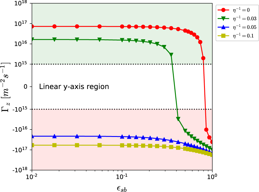
This is evident in figure 7 in the context of how  $\unicode[STIX]{x1D6E4}_{z}$ is affected by
 $\unicode[STIX]{x1D716}_{sb}$. Each curve in the figure was calculated with the Wistell-A configuration at various
 $\unicode[STIX]{x1D702}^{-1}$. The red curve is the
 $\unicode[STIX]{x1D702}^{-1}=0$ case (identical to the Wistell curve in figure 1c), where the degree of quasisymmetry is nearly good enough to retain temperature screening at such parameters. If a small density gradient
 $\unicode[STIX]{x1D702}^{-1}=0.03$ is introduced,
 $\unicode[STIX]{x1D716}_{sb}^{c}$ decreases by nearly a factor of 2. Any further increase in
 $\unicode[STIX]{x1D702}^{-1}$ pushes the plasma to the point where even perfect quasisymmetry cannot support temperature screening. This makes the situation of temperature screening even more pessimistic, because even if
 $\unicode[STIX]{x1D6E4}_{z}>0$ in a particular collisionality regime, simply introducing a density gradient can flip the sign.
The impurity particle flux for  $\text{C}^{6+}$ in Wistell-A is plotted as a function of
 $\unicode[STIX]{x1D716}_{sb}$, the scaling factor for the symmetry-breaking terms, at
 $r_{N}=0.25$. Each curve represents a different relative density gradient, but the physical parameters are otherwise identical to those of figure 1(c). The upper, green-shaded region denotes positive
 $\unicode[STIX]{x1D6E4}_{z}$ (impurity screening). The lower, red-shaded region corresponds to negative
 $\unicode[STIX]{x1D6E4}_{z}$ (impurity accumulation).

In all likelihood, there will be some finite density gradient in a reactor-relevant plasma, likely corresponding to an inward flux of impurities. It is then of interest to see how the magnitude of  $\unicode[STIX]{x1D6E4}_{z}$ changes, relative to its value at
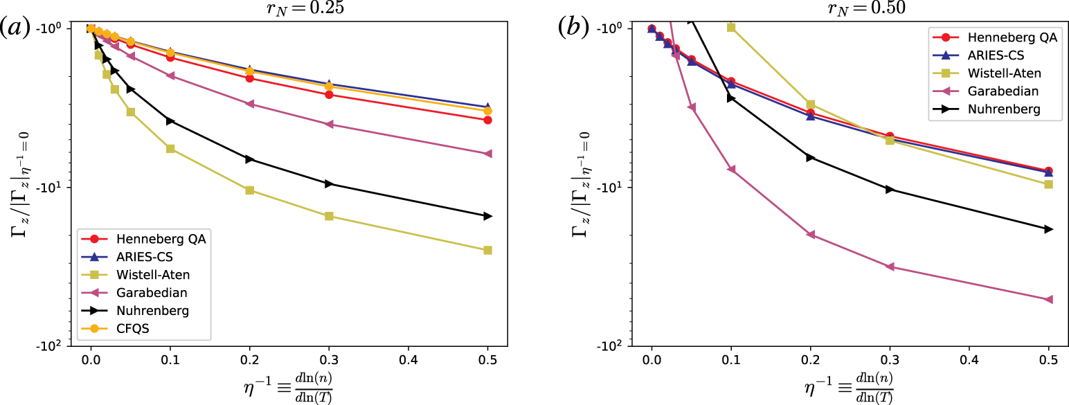
 $\unicode[STIX]{x1D702}^{-1}=0$, as the strength of the density gradient is increased. In figure 8, the ratio
 $\unicode[STIX]{x1D6E4}_{z}/|\unicode[STIX]{x1D6E4}_{z}|_{\unicode[STIX]{x1D702}^{-1}=0}$ is plotted as a function of
 $\unicode[STIX]{x1D702}^{-1}$ for various configurations, where each simulation was calculated at the true magnetic field, and used its own
 $E_{r}^{a}$. In every case shown in figure 8(a),
 $\unicode[STIX]{x1D6E4}_{z}$ is negative and a decreasing function of
 $\unicode[STIX]{x1D702}^{-1}$, indicating that increasing the strength of the peaked density gradient will intensify impurity accumulation. In a scenario where the length scale of the density gradient is only twice that of the temperature gradient
 $(\unicode[STIX]{x1D702}^{-1}=0.5)$, the enhancement in
 $\unicode[STIX]{x1D6E4}_{z}$ at this radius can be increased by a factor of
 ${\sim}20$. The picture appears to at least slightly worsen at
 $r_{N}=0.50$ in figure 8(b), where the enhanced accumulation has close to doubled from the values in figure 8(a) in most cases.
The impurity particle flux for  $\text{C}^{6+}$ has been normalized to its magnitude at
 $\unicode[STIX]{x1D702}^{-1}=0$ and plotted as a function of
 $\unicode[STIX]{x1D702}^{-1}$ at (a)
 $r_{N}=0.25$, and (b)
 $r_{N}=0.50$. Every simulation was performed at the true magnetic field
 $\unicode[STIX]{x1D716}_{sb}=1$, with the
 $E_{r}^{a}$ independently calculated at every
 $\unicode[STIX]{x1D702}^{-1}$. The physical parameters are otherwise identical to those of figures 1(c) and 3(c). The data points above
 $-10^{0}$ in (b) are those corresponding to devices with positive
 $\unicode[STIX]{x1D6E4}_{z}$ at
 $\unicode[STIX]{x1D716}_{sb}=1$, thus giving a value of
 $+10^{0}$ at
 $\unicode[STIX]{x1D702}^{-1}=0$.

6.2 Comparison to gyro-Bohm turbulence estimate
In this section, we use results from the parameter scans in the previous section to compare the neoclassical particle flux,  $\unicode[STIX]{x1D6E4}_{z}$, and heat flux,
 $Q_{total}=Q_{i}+Q_{z}$, to a gyro-Bohm estimate for turbulent transport,
 $\unicode[STIX]{x1D6E4}_{z}^{gb}\sim n_{z}D_{gb}|\unicode[STIX]{x1D735}T|/T$, and
 $Q_{total}^{gb}\sim D_{gb}|\unicode[STIX]{x1D735}T|(n_{i}+n_{z})$. In these expressions,
 $D_{gb}=\unicode[STIX]{x1D70C}_{\ast }^{2}v_{ti}a$ is the gyro-Bohm diffusion coefficient, where we have taken the minor radius to be the relevant length scale. The gyro-Bohm estimate is not a substitute for turbulent fluxes obtained from solving the gyrokinetic equation, but rather an order of magnitude estimate of the turbulence.
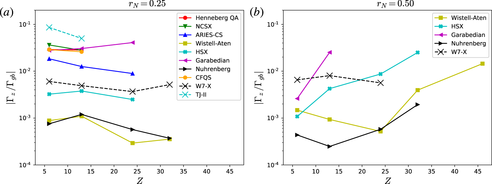
The neoclassical impurity particle flux at  $\unicode[STIX]{x1D702}^{-1}=0$ has been normalized to a gyro-Bohm estimate of the turbulent impurity particle flux (see text). This ratio is plotted as a function of the impurity charge (and mass) for (a)
 $r_{N}=0.25$, and (b)
 $r_{N}=0.50$. Plasma parameters correspond to those of figures 1(c) and 3(c). Collisionalities can be found from (a)
 $\unicode[STIX]{x1D708}_{\ast }^{z}=9.14\times 10^{-4}\;Z^{2}\;\unicode[STIX]{x1D716}^{-1}$, and (b)
 $\unicode[STIX]{x1D708}_{\ast }^{z}=1.27\times 10^{-3}\;Z^{2}\;\unicode[STIX]{x1D716}^{-1}$.

6.2.1 Impurity particle flux with $\unicode[STIX]{x1D6F7}=\unicode[STIX]{x1D6F7}_{0}(r)$

Figure 9 examines how the neoclassical particle fluxes compare to  $\unicode[STIX]{x1D6E4}_{z}^{gb}$ as a function of the impurity ion charge for each device, using the equilibrium magnetic field,
 $\unicode[STIX]{x1D716}_{sb}=1$. At
 $Z=6$, the impurities are in the plateau regime, and by
 $Z=24$ all impurities have become collisional
 $\unicode[STIX]{x1D708}_{\ast }^{z}\geqslant 1$ (depending on the aspect ratio, the
 $Z=13$ impurities are also collisional). Only flat density profiles
 $(\unicode[STIX]{x1D702}^{-1}=0)$ are considered in figure 9. In figure 9(a), we look at the impurity particle flux for
 $r_{N}=0.25$, where the temperature gradients are weaker. At this radial location, the ratio of fluxes does not have a consistent strong trend with
 $Z$. This is observed in both QA and QH configurations, as well as the non-quasisymmetric TJ-II stellarator (Hender Reference Hender1988), and the W7-X standard configuration. Note that symmetry-breaking harmonics of
 $B$ are not modified in figure 9. The most striking feature of figure 9(a), however, is the dominance of turbulent transport. Of the quasisymmetric configurations that were studied, the largest calculated neoclassical flux at
 $r_{N}=0.25$ is only
 ${\sim}5\,\%$ of the turbulent value. These small ratios indicate that regardless of whether temperature screening is present at a given collisionality, it is possible that the turbulence could control the sign of the particle flux.
At  $r_{N}=0.50$ in figure 9(b), the overall sensitivity of this ratio to the impurity species in QA is unclear since the larger gradients push
 $E_{r}^{a}$ close enough to
 $E_{r}^{res}$ that results are unreliable (see § 4). Only configurations with at least 2 points have been shown in figure 9, eliminating all but 1 QA configuration. Apart from W7-X, there is an eventual point for each configuration at which further increase in
 $Z$ corresponds to an increase in the relative importance of neoclassical fluxes. Even with this increase in the ratio, the neoclassical contribution to the radial particle flux is
 ${<}3\,\%$ of the turbulent value.
It should be reiterated here that these results have been generated with a flat density profile. While it is still unknown exactly how the density profiles will behave in a reactor, it is likely that  $|\unicode[STIX]{x1D702}^{-1}|>0$. From figure 8, it can then be inferred how this neoclassical to turbulence ratio will change if a peaked density gradient is introduced. In a non-ideal scenario, where
 $\unicode[STIX]{x1D702}^{-1}=0.5$, the ratio could increase by more than a factor of 10, depending on the configuration. At
 $r_{N}=0.25$, this would still only lead to the neoclassical flux being
 ${\sim}10\,\%$ of the turbulence for most configurations.
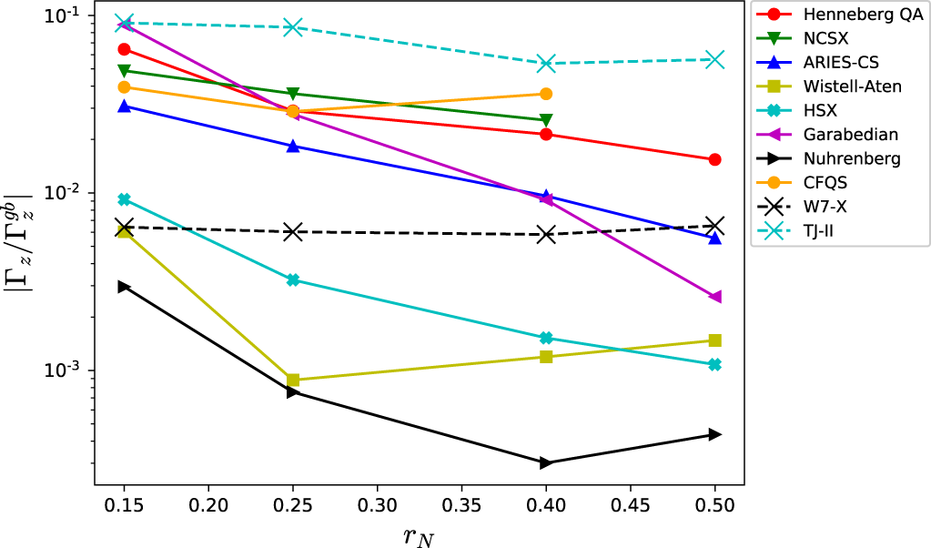
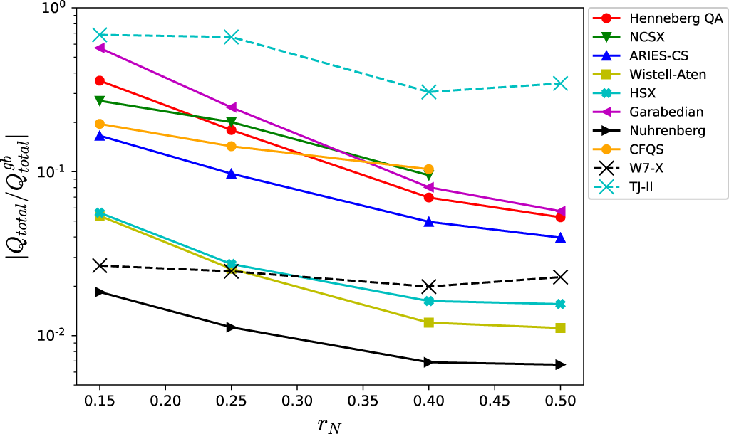
It is also of practical importance to understand how this ratio of neoclassical to turbulent particle flux varies with distance from the magnetic axis. This radial profile is shown in figure 10, where the radial points  $r_{N}=0.15$ and
 $r_{N}=0.40$ (profiles can be found in the caption of figure 10) have been added to the previously calculated values at
 $r_{N}=0.25$ and
 $r_{N}=0.50$. For most but not all, the ratio tends to either decrease or remain constant as one moves out radially, indicating that turbulence becomes increasingly more important. This follows experimental observations (Canik et al. Reference Canik, Anderson, Anderson, Clark, Likin, Talmadge and Zhai2007; Pablant Reference Pablant2018) that show neoclassical fluxes at negligible levels when compared to turbulence far from the magnetic axis.
The neoclassical impurity particle flux at  $\unicode[STIX]{x1D702}^{-1}=0$ for
 $\text{C}^{6+}$ has been normalized to a gyro-Bohm estimate of the turbulent impurity particle flux (see text). This ratio is plotted as a function of the normalized radius
 $r_{N}$. Plasma profiles at
 $r_{N}=0.25$ and
 $r_{N}=0.50$ correspond to those of figures 1(c) and 3(c), respectively. At
 $r_{N}=0.15$:
 $T=4.1~\text{keV}$,
 $\text{d}T/\text{d}r=-0.58~\text{keV}~\text{m}^{-1}$,
 $n_{i}=1.51\times 10^{20}~\text{m}^{-3}$. At
 $r_{N}=0.40$:
 $T=3.75~\text{keV}$,
 $\text{d}T/\text{d}r=-3.88~\text{keV}~\text{m}^{-1}$,
 $n_{i}=1.43\times 10^{20}~\text{m}^{-3}$.

While these results point to reactor-relevant plasmas where turbulence is likely the dominant impurity particle transport channel, more work is needed to fully understand the significance of these findings. The most obvious step would be a more accurate value for the turbulent fluxes such as a quasilinear model or gyrokinetic simulations, so as to better quantify this neoclassical to turbulence particle flux ratio. Also, a recent study comparing neoclassical simulations and experimental fluxes from an laser blow-off injection of iron in W7-X (Geiger Reference Geiger2019) similarly found that  $|\unicode[STIX]{x1D6E4}_{z}^{NC}/\unicode[STIX]{x1D6E4}_{z}^{anom}|\ll 1$. However, by separately considering the diffusive and convective contributions to the particle flux, it was found that neoclassical fluxes could still be responsible for determining the sign of the total particle transport, while the turbulence (anomalous transport) could control its magnitude.
6.2.2 Impurity particle flux including $\unicode[STIX]{x1D6F7}_{1}$ effects

The form of the DKE in (2.1) was found by linearizing about  $\unicode[STIX]{x1D6F7}_{0}$, assuming that it is close to a flux function, where
 $\unicode[STIX]{x1D6F7}_{1}\ll \unicode[STIX]{x1D6F7}_{0}$. When including
 $\unicode[STIX]{x1D6F7}_{1}$ effects, one can no longer neglect the contributions of
 $\unicode[STIX]{x1D6F7}_{1}$ in the zeroth-order distribution function
 $f_{a0}\approx F_{a}[1-Z_{a}e\unicode[STIX]{x1D6F7}_{1}/T_{a}]$, and the energy
 $W_{a}=W_{a0}+Z_{a}e\unicode[STIX]{x1D6F7}_{1}/m_{a}$, as was done in § 2.1. Furthermore, the radial component of the
 $\boldsymbol{E}\times \boldsymbol{B}$ vanishes when
 $\unicode[STIX]{x1D6F7}=\unicode[STIX]{x1D6F7}_{0}$, but enters the DKE for non-zero
 $\unicode[STIX]{x1D6F7}_{1}$, which would change the final term of § 2.1 to
 $$\begin{eqnarray}-(\boldsymbol{v}_{ma}+\boldsymbol{v}_{E})\boldsymbol{\cdot }\unicode[STIX]{x1D735}r\left(\frac{\unicode[STIX]{x2202}f_{a0}}{\unicode[STIX]{x2202}r}\right)_{W_{a}},\end{eqnarray}$$
where  $\boldsymbol{v}_{E}=(c/B^{2})\boldsymbol{B}\times \unicode[STIX]{x1D735}\unicode[STIX]{x1D6F7}_{1}$. The above replacements in the DKE will have the effect of both altering the phase space trajectories, and making the DKE nonlinear. For details on the implemented equations with
 $\unicode[STIX]{x1D6F7}_{1}$ effects see Mollén et al. (Reference Mollén, Landreman, Smith, García-Regaña and Nunami2018).
When considering  $\unicode[STIX]{x1D6F7}_{1}$ in neoclassical transport, recent results (Garcá-Regaña Reference García-Regaña2017) indicate that it has only a moderate impact on the particle flux for highly charged impurities
 $(W^{40+})$, in the case of the non-quasisymmetric Wendelstein 7-X (W7-X) stellarator. While not quasisymmetric, W7-X is still a neoclassically optimized stellarator and will have reduced radial excursions of helically trapped particles, limiting the size of density variations on a flux surface. Since
 $\unicode[STIX]{x1D6F7}_{1}$ is closely connected to these density fluctuations (Mynick Reference Mynick1984), it would make sense to assume (and indeed Garcá-Regaña (Reference García-Regaña2017) has shown) that
 $\unicode[STIX]{x1D6F7}_{1}$ fluctuations are small in such configurations. In quasisymmetric experiments not deviating too far from perfect symmetry, it is reasonable to expect a similarly small
 $\unicode[STIX]{x1D6F7}_{1}$. However, the impact of
 $\unicode[STIX]{x1D6F7}_{1}$ on the neoclassical particle flux in stellarator configurations optimized for quasisymmetry has yet to be shown. We present a first look at this behaviour using the Wistell-A configuration.
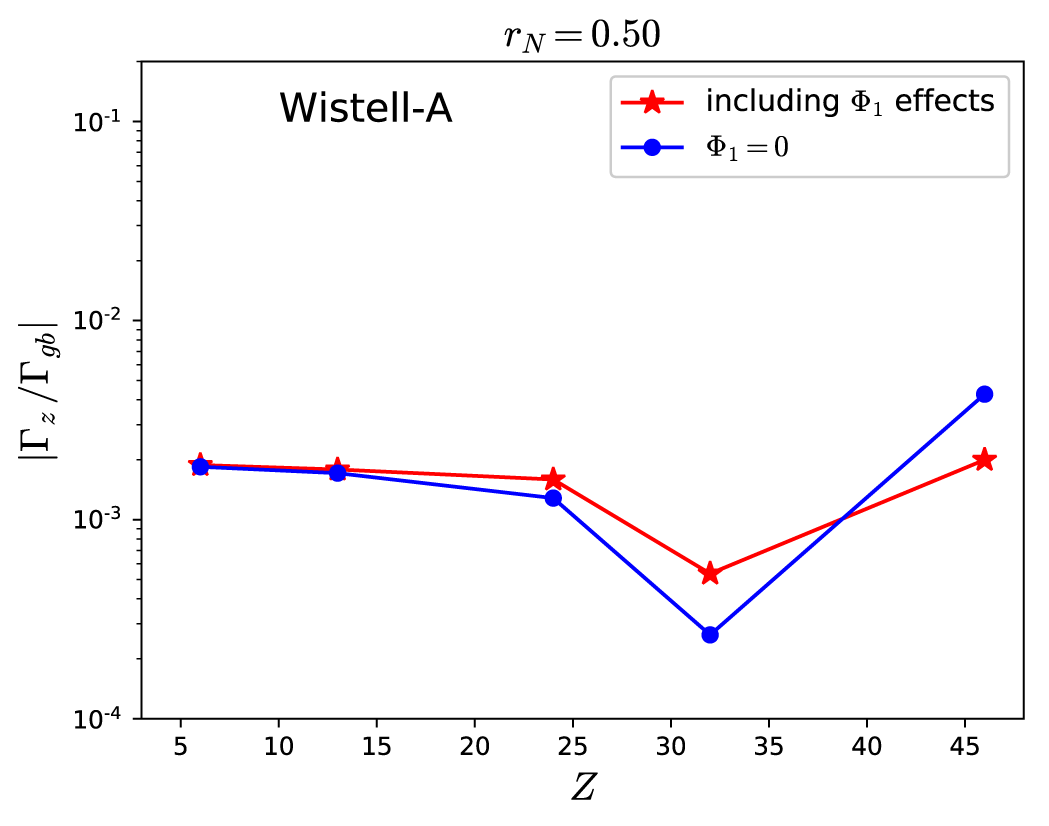
The neoclassical impurity particle flux in Wistell-A at  $\unicode[STIX]{x1D702}^{-1}=0$ has been normalized to a gyro-Bohm estimate of the turbulent impurity particle flux (see text). A kinetic electron species has been included for all points, and plasma parameters correspond to those of figure 3(c). The red curve includes
 $\unicode[STIX]{x1D6F7}_{1}$ effects in the DKE, and
 $\unicode[STIX]{x1D6F7}_{1}$ is neglected for the blue points.

In the blue curve of figure 11, we recreate the Wistell-A curve from figure 9(b), but now include a kinetic electron species (maintaining  $\unicode[STIX]{x1D6FC}=1$ and
 $\unicode[STIX]{x1D6F7}_{1}=0$). In plasmas where quasineutrality is satisfied, this permits one to solve the DKE with
 $\unicode[STIX]{x1D6F7}_{1}$ effects, which is shown in the red curve of figure 11 (where
 $E_{r}^{a}$ has been calculated at each point through the inclusion of
 $\unicode[STIX]{x1D6F7}_{1}$ effects). It is evident from figure 11, that
 $\unicode[STIX]{x1D6F7}_{1}$ has a minimal effect on impurities with low charge, especially so for
 $\text{C}^{6+}$ and
 $\text{Al}^{13+}$. However, with increasing
 $Z$, the difference in
 $\unicode[STIX]{x1D6E4}_{z}$ with and without
 $\unicode[STIX]{x1D6F7}_{1}$ effects becomes non-negligible, differing by about a factor of 2. Also of interest is the magnitude of
 $\unicode[STIX]{x1D6F7}_{1}$ fluctuations, which in our results range from
 $e|\unicode[STIX]{x1D6F7}_{1}^{max}|/T_{i}=8.9\times 10^{-4}$ to
 $e|\unicode[STIX]{x1D6F7}_{1}^{max}|/T_{i}=1.4\times 10^{-3}$, which are generally smaller than the analogous W7-X values of figure 18 in Garcá-Regaña (Reference García-Regaña2017).
Considering how our results differ from those for W7-X in Garcá-Regaña (Reference García-Regaña2017), there are some differences that must be appreciated. In Garcá-Regaña (Reference García-Regaña2017), the authors take  $\unicode[STIX]{x1D6FC}=0.1$
 $(Z_{eff}=1.1)$, and use this to solve a quasineutrality equation that does not consider the effect of the impurities on
 $\unicode[STIX]{x1D6F7}_{1}$. While this is reasonable for a low
 $Z_{eff}$ plasma, when
 $\unicode[STIX]{x1D6FC}=1$ the impurity contribution will be commensurate with bulk ions in the quasineutrality equation and their effect on
 $\unicode[STIX]{x1D6F7}_{1}$ must be considered. Second, because Wistell-A is quasisymmetric,
 $|\unicode[STIX]{x1D6E4}_{z}|$ is small in the sense that it is closer to the transition between positive and negative
 $\unicode[STIX]{x1D6E4}_{z}$ than the non-quasisymmetric W7-X. This could result in similarly sized
 $e|\unicode[STIX]{x1D6F7}_{1}^{max}|/T_{i}$ values having a comparatively stronger effect on
 $\unicode[STIX]{x1D6E4}_{z}$ in Wistell-A than in W7-X. Finally, results presented in Garcá-Regaña (Reference García-Regaña2017) employ a small but finite density gradient, where we have taken
 $\unicode[STIX]{x1D702}^{-1}=0$. As we have outlined in detail in § 6.1.2, introducing a peaked density gradient tends to have a strong influence on the impurity particle flux. Therefore, the result of introducing a density gradient alongside
 $\unicode[STIX]{x1D6F7}_{1}$ effects can be expected to modify the curves of figure 11.
It is not our aim in this section to exactly quantify the differences between our results and Garcá-Regaña (Reference García-Regaña2017). This has been meant to both introduce new results on the effect of  $\unicode[STIX]{x1D6F7}_{1}$ in a quasisymmetric geometry, and attempt to identify key differences between similar
 $\unicode[STIX]{x1D6F7}_{1}$ studies. Therefore, a more comprehensive study will be left to future work.
6.2.3 Total heat flux
Along with particle fluxes, it is also of great practical importance to compare the neoclassical and turbulent heat fluxes at different locations within the plasma. If the dominant transport channel can be identified, this can better inform future efforts in optimizing for a certain type of transport over a particular radial domain. In this section we do not distinguish between ion and impurity heat fluxes, since we primarily care about the total heat flux (ion+impurity) that is crossing a flux surface.
Thus, shifting our attention to the ratio of neoclassical to turbulent heat fluxes, the results in figure 12 show the radial profiles of this ratio for each configuration. The overall trend is similar to figure 10, except that the magnitude of this ratio is a bit higher than the respective points in figure 10, especially closer to the magnetic axis.
However, it is important to mention here that unlike the impurity particle flux, we have found this ratio to be independent of  $\unicode[STIX]{x1D702}^{-1}$, and the particular impurity species. So while the ratios in figure 10 may appear smaller in comparison, a heavy impurity in the presence of a density gradient could change that. This is to say that these heat flux ratios are more robust over a wider range of potential reactor-relevant parameters than the impurity particle flux.
The general trend of the decreasing relative importance of neoclassical heat flux compared to turbulence with respect to radius is in agreement with experimental results (Canik et al. Reference Canik, Anderson, Anderson, Clark, Likin, Talmadge and Zhai2007; Pablant Reference Pablant2018). With that said, for  $r_{N}\geqslant 0.25$, the neoclassical heat flux is, at best, 30 % of the turbulent value, and in many cases this ratio is even smaller.
These magnitudes appear to be at odds with figure 7 in Pablant (Reference Pablant2018), where neoclassical simulations (SFINCS) of an ECRH-heated W7-X experiment show that the neoclassical electron heat flux constitutes  ${\sim}65\,\%$ of the input power through the flux surface at
 $r_{N}=0.25$. If the remaining flux is presumed to be turbulence driven, then the neoclassical electron heat flux should be about twice the turbulent value. By comparing this neoclassical result to a gyro-Bohm estimate using
 $\unicode[STIX]{x1D70C}_{s}=3.21\times 10^{-3}~\text{m}$, and
 $L_{T_{e}}\equiv (1/T_{e}|\text{d}T_{e}/\text{d}r|)^{-1}=0.66~\text{m}$ in the expression
 $Q_{e}^{gb}\sim n_{e}\unicode[STIX]{x1D70C}_{\ast s}^{2}c_{s}aT_{e}L_{T_{e}}^{-1}$ one finds
 $|Q_{e}/Q_{e}^{gb}|\sim 0.05$, where
 $Q_{e}$ is the computed neoclassical electron heat flux. The above expression uses the ion sound speed
 $c_{s}=\sqrt{T_{e}/m_{i}}$ and gyroradius
 $\unicode[STIX]{x1D70C}_{s}=c_{s}/\unicode[STIX]{x1D6FA}_{i}$, where
 $\unicode[STIX]{x1D70C}_{\ast s}\equiv \unicode[STIX]{x1D70C}_{s}/a$. A similar comparison can be done for HSX with figure 13 in Canik et al. (Reference Canik, Anderson, Anderson, Clark, Likin, Talmadge and Zhai2007), where the neoclassical electron thermal diffusivity appears to account for
 ${\sim}10\,\%$ of the experimentally measured diffusivity at
 $r_{N}=0.25$. Using the above approximation for
 $Q_{e}^{gb}$, with length scales
 $\unicode[STIX]{x1D70C}_{s}=3.42\times 10^{-3}~\text{m}$ and
 $L_{T_{e}}=0.042~\text{m}$, results in
 $|Q_{e}/Q_{e}^{gb}|\sim 0.02$.
These inconsistencies in how well gyro-Bohm approximates the turbulence underlines the nature of gyro-Bohm as only an estimate of turbulence.
Setting the coefficient of  $D_{gb}$ to
 $1$ for every configuration and set of plasma parameters is bound to yield results that can differ by an appreciable amount relative to the actual turbulent fluxes.
It should be mentioned that for the above cases,  $T_{e}\gg T_{i}$, indicating that electrons will likely be important for both neoclassical and turbulent energy transport. This is in contrast to the majority of results in our work, where electrons were excluded from simulations. For plasmas with large
 $T_{e}/T_{i}$, the ion temperature gradient is no longer the relevant driving gradient, which is why
 $c_{s}$ and
 $\unicode[STIX]{x1D70C}_{s}$ have been used in
 $Q_{e}^{gb}$ above, in place of
 $v_{ti}$ and
 $\unicode[STIX]{x1D70C}_{i}$. While the HSX result in particular is interesting in the sense that it is the only experimental quasisymmetric stellarator data comparing transport channels, it is unclear of how relevant it is to the rest of the results in this paper, considering that
 $T_{e}\gg T_{i}$.
The total (ion  $+$ impurity) heat flux at
 $\unicode[STIX]{x1D702}^{-1}=0$ for
 $\text{C}^{6+}$ has been normalized to a gyro-Bohm estimate of the total turbulent heat flux (see text). This ratio is plotted as a function of the normalized radius
 $r_{N}$. Plasma profiles are the same as for figure 10.

7 Effective helical ripple as a quasisymmetry metric
From § 6.1, we showed how there was a connection between  $S$ and
 $\unicode[STIX]{x1D716}_{sb}^{c}$ that helped to explain how
 $\unicode[STIX]{x1D716}_{sb}^{c}$ changed between the two flux surfaces that were studied. This connection can be seen more clearly in figure 13(a,b), where the value of
 $\unicode[STIX]{x1D716}_{sb}^{c}$ from figures 1(a) and 3(a) has been plotted as a function of
 $S$ on the respective surfaces for each of the configurations. For both
 $r_{N}=0.25$ and
 $r_{N}=0.50$, there is a visible anti-correlation between the two quantities even when considering that these configurations have very different properties. It thus seems reasonable to expect that minimizing
 $S$ on a flux surface will increase
 $\unicode[STIX]{x1D716}_{sb}^{c}$.
The critical symmetry-breaking parameter  $\unicode[STIX]{x1D716}_{sb}^{c}$ for each configuration as a function of the corresponding
 $S$ value has been plotted at (a)
 $r_{N}=0.25$, and (b)
 $r_{N}=0.50$, which correspond to the
 $\unicode[STIX]{x1D716}_{sb}^{c}$ values from figures 1(a) and 3(a), respectively.

Along with  $S$, the effective helical ripple,
 $\unicode[STIX]{x1D716}_{eff}$, is sometimes taken to be a metric for quasisymmetry that could be used for stellarator optimization;
 $\unicode[STIX]{x1D716}_{eff}$, which is a measure of neoclassical transport in the
 $1/\unicode[STIX]{x1D708}$ regime, was computed with the NEO code (Nemov et al. Reference Nemov, Kasilov, Kernbichler and Heyn1999).
The effective helical ripple (calculated with NEO (Nemov et al. Reference Nemov, Kasilov, Kernbichler and Heyn1999)) is plotted as a function of the amplitude of the symmetry-breaking terms. The open circles here denote the value on-axis ( $r_{N}=0$). The closed circles correspond to the value at
 $r_{N}=1$. These curves do not change with plasma parameters.

In figure 14, the effective helical ripple is plotted as a function of  $S$ for each configuration. A number of these curves are multi-valued, indicating a non-monotonic change in quasisymmetry from the magnetic axis to the last closed flux surface (LCFS). To clarify the radial dependency of each curve, the open circle at the end of a curve denotes the magnetic axis,
 $r_{N}=0$, and a closed circle the LCFS,
 $r_{N}=1$. It can be seen (Mynick, Boozer & Ku Reference Mynick, Boozer and Ku2006; Henneberg et al. Reference Henneberg, Drevlak, Nührenberg, Beidler, Turkin, Loizu and Helander2019) that if individual symmetry-breaking
 $B_{mn}$ harmonics are plotted as a function of
 $r_{N}$, that the amplitude tends to increase with distance from the magnetic axis. Indeed, this trend can be seen for a handful of configurations in figure 14, indicating a correlation between
 $\unicode[STIX]{x1D716}_{eff}$ and the closeness to quasisymmetry. However, this is decidedly not universal among QA configurations. Henneberg QA, for example, has a symmetry-breaking amplitude that decreases by nearly an order of magnitude from
 $r_{N}=0\rightarrow r_{N}\simeq 0.6$, and then increases again to a value at
 $r_{N}=1$ that is larger than its value at the
 $r_{N}=0$.
Moreover, this monotonicity in  $S$, or lack thereof, is not necessarily tied to the value of
 $\unicode[STIX]{x1D716}_{eff}$. Returning to Henneberg QA as an example, the initial decrease in
 $S$ with
 $r_{N}$ is accompanied with a decrease in
 $\unicode[STIX]{x1D716}_{eff}$. Then, the subsequent increase in
 $S$ corresponds to an increase in
 $\unicode[STIX]{x1D716}_{eff}$, indicating a possible correlation between
 $S$ and
 $\unicode[STIX]{x1D716}_{eff}$. However, the behavior is different in the core of ARIES-CS, where the smallest value of
 $S$ corresponds to a relatively large value of
 $\unicode[STIX]{x1D716}_{eff}$, which decreases considerably as
 $S$ is increased. The point here is that while there are certainly configurations where
 $\unicode[STIX]{x1D716}_{eff}$ scales with
 $S$, it is just as likely that they may not correlate well at all, and the assumption that small
 $\unicode[STIX]{x1D716}_{eff}$ indicates good quasisymmetry cannot be justified a priori. It has in fact been shown in Cary & Shasharina (Reference Cary and Shasharina1997) that one can achieve omnigeneity
 $(\unicode[STIX]{x1D716}_{eff}=0)$ far from quasisymmetry.
It is further interesting to note that in the cases where  $\unicode[STIX]{x1D716}_{eff}$ does not scale with
 $S$, the radial location where this disagreement happens is usually within
 $r_{N}\simeq 0.5$. Above this
 $r_{N}$ (or in some configurations, a position much closer to the magnetic axis), the scaling of
 $\unicode[STIX]{x1D716}_{eff}$ with
 $S$ can be observed in every case. An interpretation of this behaviour is left to future work.
8 Conclusions
In this work, we have examined how impurity particle flux and the temperature screening effect are influenced by varying the closeness of the magnetic field to perfect quasisymmetry. For realistic departures from symmetry, at the lowest studied collisionality (both species in the  $\sqrt{\unicode[STIX]{x1D708}}$ regime) with a flat density gradient, temperature screening was not observed for any quasisymmetric configuration. However, with increasing collisionality one can see an increase in the ‘effective quasisymmetry’ of a flux surface. This can lead to temperature screening in some cases. Unfortunately, there is an upper limit to the benefits of increasing collisionality, where any further increase will lead to impurity accumulation even in perfect quasisymmetry.
When peaked density gradients are introduced, there is an overall negative effect on the impurity particle flux. Increasing the density gradient peaking  $(\unicode[STIX]{x1D702}^{-1}>0)$ enhances the strength of the impurity accumulation, and also leads to a reduction in the ‘effective quasisymmetry’. Overall, while temperature screening is technically possible at the true magnetic field in select cases, it is unlikely to be present in low-collisionality reactor-relevant regimes.
The magnitudes of these results at the true magnetic field ( $\unicode[STIX]{x1D716}_{sb}=1$) were then compared to a gyro-Bohm estimate for the turbulent fluxes. Even in the non-ideal scenario of
 $\unicode[STIX]{x1D702}^{-1}=0.5$, the majority of configurations show neoclassical impurity particle fluxes that do not exceed 10 % of the respective turbulent flux, even for highly charged impurities. However, a complete understanding of the implications of a relatively large turbulent particle flux will require further work, since determining sign of the particle flux may be more complicated than taking the sign of the largest transport channel (Geiger Reference Geiger2019). In other words, while neoclassical fluxes may potentially be small, they cannot be considered irrelevant.
It was also found that when studying highly charged impurities in Wistell-A in relevant  $Z_{eff}$ plasmas, one cannot disregard the effect that including
 $\unicode[STIX]{x1D6F7}_{1}$ can have on
 $\unicode[STIX]{x1D6E4}_{z}$. Even though the effect on
 $\unicode[STIX]{x1D6E4}_{z}$ is considerable, the absolute value of
 $\unicode[STIX]{x1D6F7}_{1}$ is quite small, indicating that its relationship to
 $\unicode[STIX]{x1D6E4}_{z}$ is more complicated than just considering its magnitude.
Finally, it was shown that the critical value of symmetry breaking,  $\unicode[STIX]{x1D716}_{sb}$, where the impurity particle flux changes sign, appears to be anti-correlated with the amplitude of symmetry-breaking harmonics,
 $S$, on a flux surface. That this trend appears when considering configurations with widely varying properties suggests that minimizing the
 $S$ on a flux surface will increase
 $\unicode[STIX]{x1D716}_{sb}$.
Acknowledgements
The authors would like to thank S. Henneberg for providing the configuration in Henneberg et al. (Reference Henneberg, Drevlak, Nührenberg, Beidler, Turkin, Loizu and Helander2019), A. Bader for providing Wistell-A, J. Schmitt for providing HSX, N. Pomphrey for providing NCSX and ARIES-CS and S. Okamura for providing CFQS. We would also like to thank I. Abel, A. Geraldini, R. Jorge and E. Paul for useful comments and discussions. This work was supported by the U.S. Department of Energy, Office of Science, Office of Fusion Energy Science, under award DE-FG02-93ER54197. This research used resources of the National Energy Research Scientific Computing Center (NERSC), a U.S. Department of Energy Office of Science User Facility operated under contract no. DE-AC02-05CH11231.
Editor Per Herlander thanks the referees for their advice in evaluating this article.
Appendix A. Impurity temperature screening in axisymmetry and quasisymmetry
A number of papers (Galeev & Sagdeev Reference Galeev and Sagdeev1968; Rosenbluth, Hazeltine & Hinton Reference Rosenbluth, Hazeltine and Hinton1972; Connor Reference Connor1973; Rutherford Reference Rutherford1974) have examined neoclassical transport quantities in the axisymmetric limit and can provide a more intuitive look at the properties of a plasma that can affect temperature screening. These results are also applicable in perfect quasisymmetry. In Connor (Reference Connor1973), an expression for the bulk ion (taken to be hydrogen here) particle flux in the presence of electrons and a single impurity was derived, using a momentum-conserving, pitch-angle scattering collision operator, where all species are taken to be in the banana regime
 $$\begin{eqnarray}\unicode[STIX]{x1D6E4}_{i}=-C_{i}\left\{\frac{T_{i}}{T_{e}}\left[\frac{n_{i}^{\prime }}{n_{i}}-\left(\frac{0.09+0.5\unicode[STIX]{x1D6FC}}{0.53+\unicode[STIX]{x1D6FC}}\right)\frac{T_{i}^{\prime }}{T_{i}}\right]-\frac{T_{z}}{ZT_{e}}\left[\frac{n_{z}^{\prime }}{n_{z}}-0.17\frac{T_{z}^{\prime }}{T_{z}}\right]\right\}.\end{eqnarray}$$
Here,  $C_{i}$ is a positive coefficient that is independent of thermodynamic gradients,
 $Z$ is the impurity charge and
 $\unicode[STIX]{x1D6FC}=n_{z}Z^{2}/n_{i}=Z_{eff}-1$ represents the effect of the impurities on the transport coefficients. Typically, one can take
 $T_{i}=T_{z}=T$, and we further assume the profiles of each species to be equal:
 $T_{i}^{\prime }/T_{i}=T_{z}^{\prime }/T_{z}=T^{\prime }/T$, and
 $n_{i}^{\prime }/n_{i}=n_{z}^{\prime }/n_{z}=n^{\prime }/n$. An expression for the impurity particle flux can then easily be obtained by satisfying the ambipolarity condition,
 $\sum _{a}Z_{a}\unicode[STIX]{x1D6E4}_{a}=0$. Based on
 $\unicode[STIX]{x1D6E4}_{e}\sim \sqrt{m_{e}/m_{i}}\,\unicode[STIX]{x1D6E4}_{i}$, if we take
 $\unicode[STIX]{x1D6E4}_{e}\simeq 0$, then
 $\unicode[STIX]{x1D6E4}_{z}\simeq -\unicode[STIX]{x1D6E4}_{i}/Z$. The impurity particle flux can now be shown to be
 $$\begin{eqnarray}\unicode[STIX]{x1D6E4}_{z}=\frac{C_{i}}{Z}\left\{\frac{T}{ZT_{e}}\left[L_{a}\frac{n^{\prime }}{n}-L_{b}\frac{T^{\prime }}{T}\right]\right\},\end{eqnarray}$$
where  $L_{a}\equiv Z-1$ and
 $L_{b}\equiv \{[Z(0.09+0.5\unicode[STIX]{x1D6FC})/(0.53+\unicode[STIX]{x1D6FC})]-0.17\}$;
 $L_{b}$ is always positive for
 $Z>1$.
If it is assumed that both density and temperature profiles are peaked, then achieving a positive (outward)  $\unicode[STIX]{x1D6E4}_{z}$ is based on two properties:
 $Z_{eff}$, and more importantly, the ratio
 $\unicode[STIX]{x1D702}^{-1}\equiv d\ln (n)/d\ln (T)$. In the absence of a density gradient, the term in square brackets in (A 2) will always be positive and lead to temperature screening. However, based on the
 $\unicode[STIX]{x1D6FC}$, there is some critical
 $\unicode[STIX]{x1D702}_{c}^{-1}(\unicode[STIX]{x1D6FC})\sim 0.4$ where
 $\unicode[STIX]{x1D702}^{-1}>\unicode[STIX]{x1D702}_{c}^{-1}$ will always lead to impurity accumulation. This effect can be seen in figure 15, where SFINCS has been used to calculate the impurity particle flux for
 $\text{C}^{6+}$ over a range of collisionalities for an axisymmetric geometry model
 $B(\unicode[STIX]{x1D703})=B_{0}(1+\unicode[STIX]{x1D716}\cos \unicode[STIX]{x1D703})$, with
 $\unicode[STIX]{x1D704}=0.689$ and
 $\unicode[STIX]{x1D6FC}=1$. It is also clear that temperature screening is only accessible up to some maximum collisionality, regardless of
 $\unicode[STIX]{x1D702}^{-1}$. However, such high collisionalities put not only impurities, but also bulk ions, into the Pfirsch–Schlüter regime, which is generally too collisional to be relevant in the core of reactor scenarios.
The impurity particle flux for  $\text{C}^{6+}$ is plotted in an axisymmetric geometry as a function of the normalized ion–ion collisionality
 $\unicode[STIX]{x1D708}_{\ast }^{ii}\equiv \unicode[STIX]{x1D708}R/v_{ti}$, where
 $\unicode[STIX]{x1D716}=r_{N}(a/R)$. In this plot,
 $r_{N}=0.25$, and
 $a/R=0.16$. The vertical lines signify the transitions between collisionality regimes for
 $\unicode[STIX]{x1D708}_{\ast }^{ii}$ (black dashed) and
 $\unicode[STIX]{x1D708}_{\ast }^{zz}$ (magenta dotted). The transitions are as follows:
 $\unicode[STIX]{x1D708}_{\ast }^{ii}=1.41\times 10^{-3}$ (main ion banana plateau),
 $\unicode[STIX]{x1D708}_{\ast }^{ii}=0.18$ (main ion plateau Pfirsch–Schlüter),
 $\unicode[STIX]{x1D708}_{\ast }^{ii}=3.93\times 10^{-5}$ (impurity banana plateau) and
 $\unicode[STIX]{x1D708}_{\ast }^{ii}=5.03\times 10^{-3}$ (impurity plateau Pfirsch–Schlüter). The upper, green-shaded region denotes positive
 $\unicode[STIX]{x1D6E4}_{z}$ (impurity screening). The lower, red-shaded region corresponds to negative
 $\unicode[STIX]{x1D6E4}_{z}$ (impurity accumulation).