1 Introduction
Similarity solutions play a central role in fluid mechanics (Barenblatt Reference Barenblatt2003). Many problems in fluid mechanics lead to nonlinear partial differential equations in space and time for unknown quantities such as velocity components, concentrations, depth of fluid flow,
 $\ldots$
. Examples include: numerous boundary layer problems; the initial stages of nuclear explosions; the infiltration of ground water; the relaxation of a surface-tension dominated volume of carbon dioxide sequestered at depth in a porous geological sequence; the osmotic flow of solvent across a membrane; and diffusion of granular media, to name but a few situations.
The resulting equations very rarely have analytical solutions and hence resort to numerical calculations is essential. Numerical investigation of the influence of each of the parameters, and possible different initial conditions, would be time consuming and need quite intricate numerical programming. Very often, at least within the problems tackled and solved, a similarity form of solution exists whereby the partial differential equation is transformed into an ordinary differential equation (but still nonlinear), the solutions to which do not obey the particular initial conditions. It is then confidentially asserted that all solutions approach this similarity form. But what is the time taken to do so? This is almost always thought to be a difficult problem and is generally stated as: the solutions will be valid for
 $t\gg t_{\ast }$
, where
 $t_{\ast }$
is some suitable time scale (but how does it depend on the parameters of the problem?). Of course there are some problems where the solutions to the initial-value problems do not approach the similarity solutions (Acton, Huppert & Worster Reference Acton, Huppert and Worster2001; Johnson et al.
Reference Johnson, Hogg, Huppert, Sparks, Phillips, Slim and Woodhouse2015) or only for special values of the physical parameters.
The point of this paper is to present the equilibration time for the particular case of a viscous gravity current developing from an initially constrained volume of fluid
 $V$
. The ideas presented no doubt have much greater applicability; and informal discussions with fluid-mechanical colleagues have already suggested a number of different examples.
Gravity currents occur wherever fluid of one density flows primarily horizontally into fluid of a different density (Simpson Reference Simpson1997; Huppert Reference Huppert2006). Many different fundamental fluid mechanical cases exist including: axisymmetric and two-dimensional geometries; constant volume or constant flux releases; and propagation at low or high Reynolds number. This paper will concentrate initially on the instantaneous release of a constant volume of viscous fluid over a horizontal surface (Huppert Reference Huppert1982) and then discusses in the appendix A the implications of the results for other geometries and situations.
Assuming both that the horizontal scale greatly exceeds the vertical scale, so that the pressure is hydrostatic, and that the Bond number
 $B=\unicode[STIX]{x0394}\unicode[STIX]{x1D70C}gl^{2}/T\gg 1$
, where
 $\unicode[STIX]{x0394}\unicode[STIX]{x1D70C}$
is the density difference between intruding and intruded fluid,
 $g$
is gravity,
 $l$
a horizontal scale of the current (such as its radius) and
 $T$
is surface tension, Huppert (Reference Huppert1982) determines that the radial horizontal component of the velocity
 $u(r,t)$
, where
 $r$
is radius and
 $t$
time, is parabolic in the vertical component
 $z$
, except close to the front of the current, which for
 $B\gg 1$
plays a negligible role. The height of the unknown free surface
 $h(r,t)$
then satisfies
 $$\begin{eqnarray}\frac{\unicode[STIX]{x2202}h}{\unicode[STIX]{x2202}t}-\frac{\unicode[STIX]{x1D6FD}}{r}\frac{\unicode[STIX]{x2202}}{\unicode[STIX]{x2202}r}\left(rh^{3}\frac{\unicode[STIX]{x2202}h}{\unicode[STIX]{x2202}r}\right)=0,\end{eqnarray}$$
where
 $$\begin{eqnarray}\unicode[STIX]{x1D6FD}=g\unicode[STIX]{x0394}\unicode[STIX]{x1D70C}/(3\unicode[STIX]{x1D707})\end{eqnarray}$$
and
 $\unicode[STIX]{x1D707}$
the dynamic viscosity of the intruding fluid, with boundary and global conditions,
 $$\begin{eqnarray}h(r_{S})=0\quad \text{and}\quad 2\unicode[STIX]{x03C0}\int _{0}^{r_{S}(t)}rh(r,t)\,\text{d}r=V,\end{eqnarray}$$
where
 $r_{S}(t)$
is the radial extent of the current.
An appropriate similarity variable, determined by balancing terms in (1.1) and (1.3), or otherwise, is given by
 $$\begin{eqnarray}\unicode[STIX]{x1D709}=(\unicode[STIX]{x1D6FD}V^{3})^{-1/8}rt^{-1/8},\end{eqnarray}$$
with the form of
 $h(r,t)$
given by
 $$\begin{eqnarray}h(r,t)=\unicode[STIX]{x1D709}_{S}^{2/3}(V/\unicode[STIX]{x1D6FD})^{1/4}t^{-1/4}\unicode[STIX]{x1D713}(z\equiv \unicode[STIX]{x1D709}/\unicode[STIX]{x1D709}_{S}),\end{eqnarray}$$
where
 $\unicode[STIX]{x1D709}_{S}$
is the value of
 $\unicode[STIX]{x1D709}$
at
 $r=r_{S}(t)$
given by
 $$\begin{eqnarray}r_{S}(t)=\unicode[STIX]{x1D709}_{S}(\unicode[STIX]{x1D6FD}V^{3})^{1/8}t^{1/8}.\end{eqnarray}$$
Substituting (1.4) and (1.5) into (1.1) and (1.3), Huppert (Reference Huppert1982) finds that
 $\unicode[STIX]{x1D713}(z)$
satisfies
 $$\begin{eqnarray}(z\unicode[STIX]{x1D713}^{3}\unicode[STIX]{x1D713}^{\prime })^{\prime }+{\textstyle \frac{1}{8}}z^{2}\unicode[STIX]{x1D713}^{\prime }+{\textstyle \frac{1}{4}}\unicode[STIX]{x1D713}=0\end{eqnarray}$$
and
 $$\begin{eqnarray}\unicode[STIX]{x1D709}_{S}=\left[2\unicode[STIX]{x03C0}\int _{0}^{1}z\unicode[STIX]{x1D713}(z)\,\text{d}z\right]^{-3/8},\end{eqnarray}$$
the analytical solution to which is (Pattle Reference Pattle1959; Huppert Reference Huppert1982)
 $$\begin{eqnarray}\unicode[STIX]{x1D713}(z)=(3/16)^{1/3}(1-z^{2})^{1/3}\end{eqnarray}$$
and
 $$\begin{eqnarray}\unicode[STIX]{x1D709}_{S}=(2^{10}/3^{4}\unicode[STIX]{x03C0}^{3})^{1/8}=0.894\ldots .\end{eqnarray}$$
The aspect ratio
 $\unicode[STIX]{x1D6FE}\equiv h(0,t)/r_{S}(t)$
, evaluated from (1.5), (1.6), (1.9) and (1.10), is hence given by
 $$\begin{eqnarray}\unicode[STIX]{x1D6FE}=0.594(\unicode[STIX]{x1D6FD}^{3}V)^{-1/8}t^{-3/8}.\end{eqnarray}$$
Laboratory experiments conducted to demonstrate the validity of the approach, in particular the neglect of contact line effects at the front, showed, for a variety of initial geometries, including different shaped cylinders and rapidly pouring the fluid on a horizontal base, that the relationship was very closely observed, over time scales in the laboratory from 10 s to several weeks. We mention in passing, that the influence of rapid rotation, small Rossby number, is quite different, leading to thin radially extending fingers (Dalziel & Huppert Reference Dalziel and Huppert2019).
The question to be addressed here is exactly how quickly does the initial-value problem approach this similarity solution from an arbitrary initial condition, specifying some axisymmetric initial distribution of
 $h(r,0)$
enclosing a volume
 $V$
? The result will clearly depend on the parameters of the problem:
 $\unicode[STIX]{x0394}\unicode[STIX]{x1D70C},g,\unicode[STIX]{x1D707},V$
and the initial (supposed axisymmetric) distribution of
 $h(r,0)$
. Any easy-to-do experiment in the laboratory illustrating this problem shows that departures from axisymmetry are quickly eliminated, as suggested by the late-time linear analyses of Grundy & Rottman (Reference Grundy and Rottman1985). The first three parameters occur together in (1.1) in the variable
 $\unicode[STIX]{x1D6FD}=g\unicode[STIX]{x0394}\unicode[STIX]{x1D70C}/(3\unicode[STIX]{x1D707})$
, with dimensions of
 $L^{-1}T^{-1}$
. The volume
 $V$
has dimensions
 $L^{3}$
. Therefore the only variable with dimensions of time is proportional to
 $\unicode[STIX]{x1D6E4}\equiv 1/(V^{1/3}\unicode[STIX]{x1D6FD})$
. It thus seems reasonable to assume that the equilibration time is linearly proportional to
 $\unicode[STIX]{x1D6E4}$
, with the constant dependent on the initial configuration of
 $V$
.
Our numerical results, described in the next section, confirm this result. But how does this time depend on shape, and also on configuration? Does an initially cylindrical shape approach the similarity solution faster or slower than say a conical initial shape, both of the same volume
 $V$
? How does an initial condition of an inverted cone compare? Do the comparisons depend on how close to the similarity solution is considered? What initial shape approaches the similarity solution fastest/slowest?
We determine a full relationship for the time of equilibration
 $\unicode[STIX]{x1D70F}$
as a function of the initial aspect ratio first for an initially circular cylinder and then compare this to the time scale for other initial shapes. Possibly surprisingly, taller initial shapes (with the same volume) approach the (relatively small height and small slope) similarity solution more rapidly. This result is clearly explained in the next section. It should be noted, however, that the time scale
 $\unicode[STIX]{x1D70F}$
is relevant for the numerical solution of (1.1) to approach the similarity solution (1.6), and not the collapse of an initial set-up with non-small slopes.
However, we have not yet defined exactly the equilibration time
 $\unicode[STIX]{x1D70F}$
as a function of
 $p$
the percentage agreement. We could choose the agreement between the radius of the similarity solution and the exact nonlinear solution (which we shall do), or other, possibly equally convenient, definitions, such as based on the (difference of) values (of height) at the centre, some mean difference along the whole profile,
 $\ldots$
. Each of these last two spelt-out possibilities have obvious disadvantages: either the height at the centre may (for all time) not well reflect the form of solution or the evaluation involves an extra, somewhat tricky, integration to determine mean differences. A discrepancy based on the radius is simple, direct and easiest to measure in the laboratory or evaluate numerically.
We expect that
 $\unicode[STIX]{x1D70F}$
is infinite for zero
 $p$
, and a monotonically decreasing function of
 $p$
(it should take less time to be less accurate). However, as
 $p$
approaches 0 does
 $\unicode[STIX]{x1D70F}$
increase: exponentially; like a power law; logarithmically; or
 $\ldots$
? The answer, at least for this problem, seems to be as the inverse of
 $p$
. For a completely different problem in detail, it could be different. For example, Grundy & Rottman (Reference Grundy and Rottman1985) state that for the equivalent problem of a high Reynolds number gravity current the corresponding shallow water equations have a similarity solution which is approached in an oscillatory manner. This different case is discussed fully in a companion paper by Webber & Huppert (Reference Webber and Huppert2019).
2 Numerical evaluations
We employed a numerical program to solve (1.1) subject to a variety of initial conditions,
 $h(r,0)$
. The program uses a Crank–Nicolson predictor–corrector scheme where spatial gradients are evaluated by central differences. To reduce computational cost, the finite difference scheme is combined with adaptive grid size and time stepping.
Preliminary runs with both a circular cylinder and a hemisphere lead to similarly smooth results – we were worried that the discontinuities in height associated with a cylinder might lead to unreliable results – and so we initially opted mainly for the simpler initial condition of a right cylinder of radius
 $r_{0}$
and height
 $h_{0}$
(with initial aspect ratio
 $\unicode[STIX]{x1D6FE}_{0}=h_{0}/r_{0}$
and volume
 $V=\unicode[STIX]{x03C0}h_{0}r_{0}^{2}=\unicode[STIX]{x03C0}\unicode[STIX]{x1D6FE}_{0}r_{0}^{3}$
). The first set of runs was undertaken with
 $h_{0}=r_{0}=1$
for various values of
 $\unicode[STIX]{x1D6FD}$
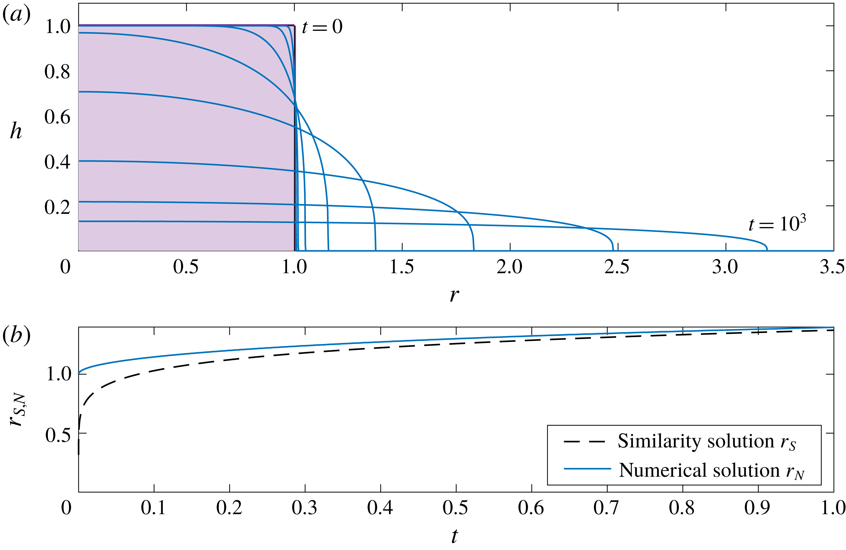
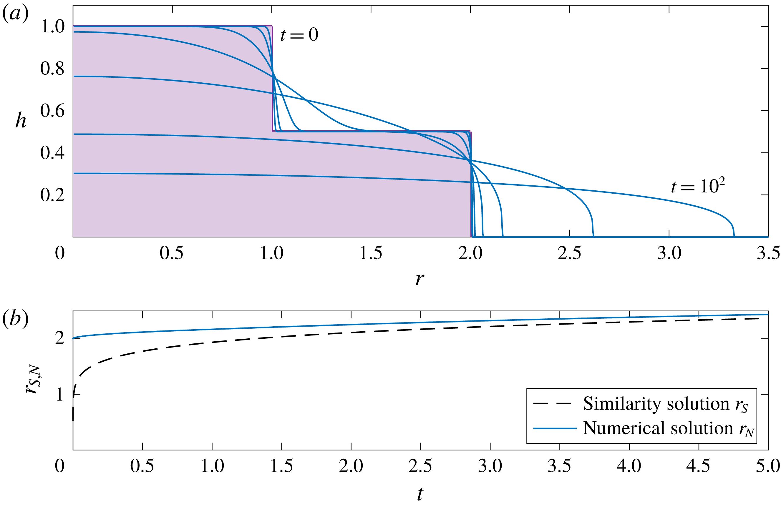
. Figure 1 shows the resulting shapes and a comparison between the numerically determined radial extent
 $r_{N}$
and the similarity solution
 $r_{S}$
for
 $\unicode[STIX]{x1D6FD}=1$
. The numerically evaluated radii as functions of time normalised by
 $\unicode[STIX]{x1D6FD}^{1/8}$
(cf. (1.6)) for various values of
 $\unicode[STIX]{x1D6FD}$
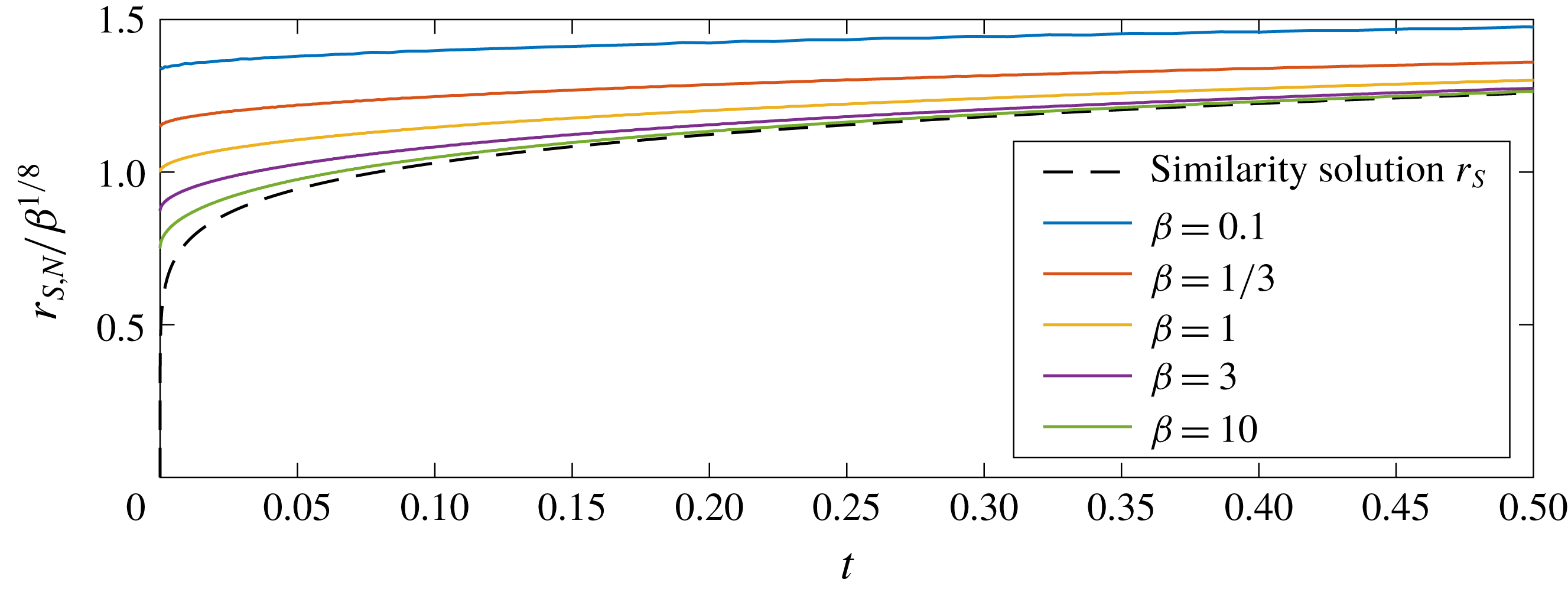
are shown in figure 2, which also displays the similarity solution (1.6). The numerically determined radius, whose initial value is 1, is always in excess of that for the similarity solution, for which the initial value is zero. (But see a different interpretation discussed at the end of this section). The numerical radii approached those given by the similarity solution (1.7) as
 $t^{-7/8}$
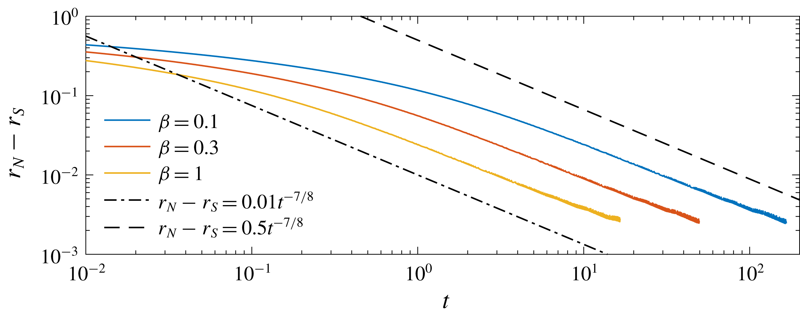
, the temporal derivative of (1.6), as shown in figure 3 for various values of
 $\unicode[STIX]{x1D6FD}$
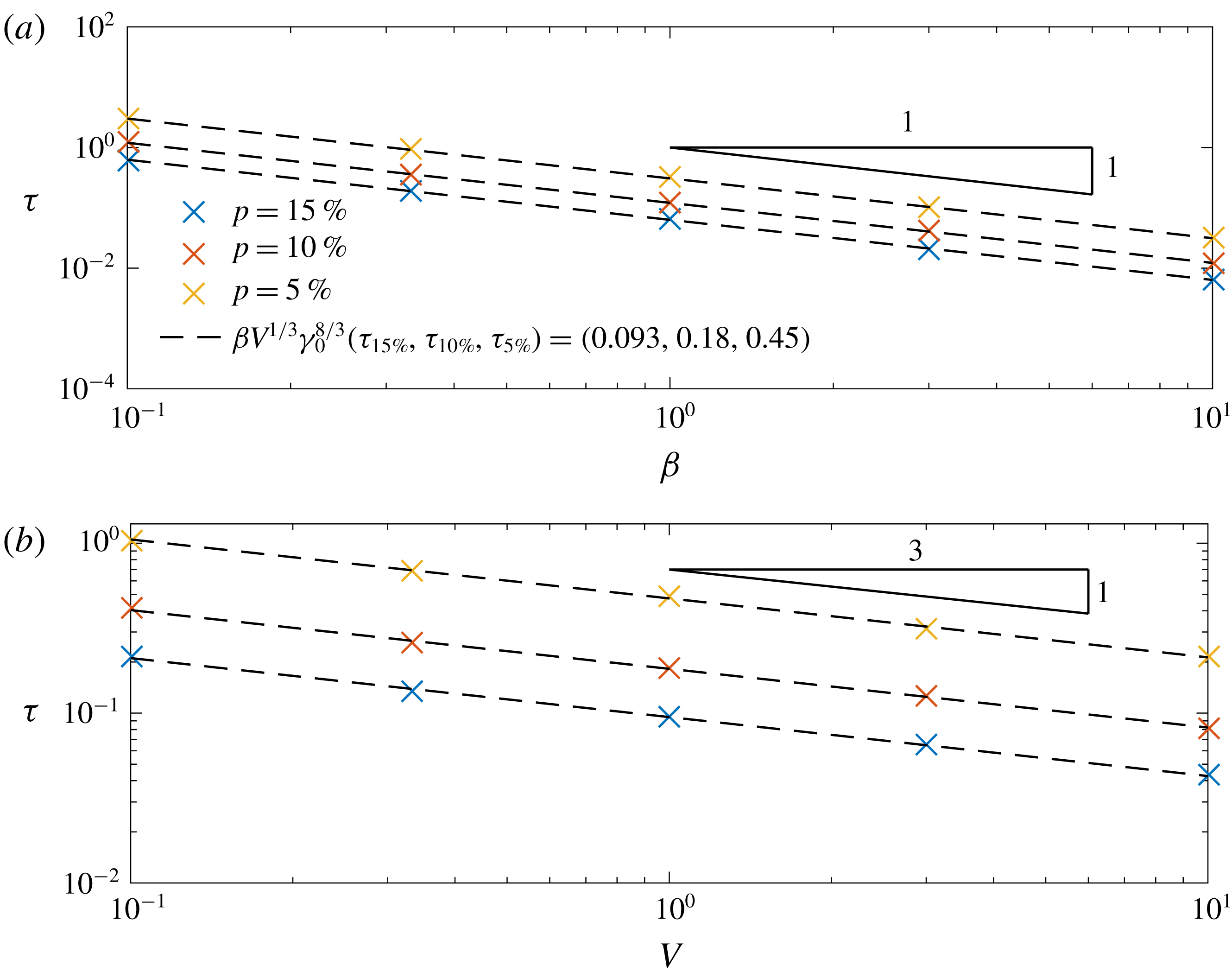
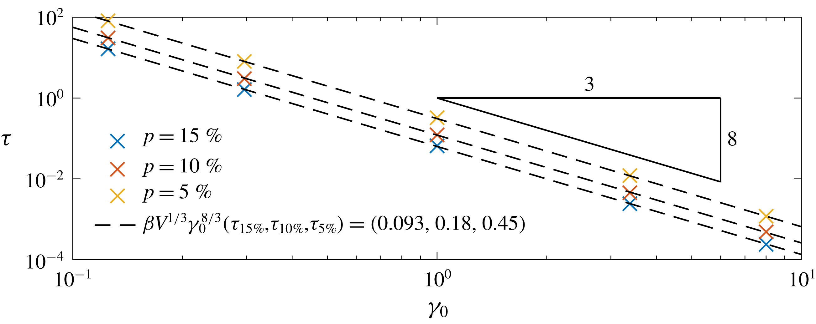
. Figure 4(a) presents the time
 $\unicode[STIX]{x1D70F}$
taken for the numerically evaluated radius to be within 15 %, 10 %, 5 % of the similarity solution as a function of
 $\unicode[STIX]{x1D6FD}$
. This confirms that, as predicted,
 $\unicode[STIX]{x1D70F}$
varies inversely with
 $\unicode[STIX]{x1D6FD}$
(for fixed initial conditions), and acts as a check of the validity and accuracy of the numerical program. It also indicates that for a circular cylinder of initial unit height and radius,
 $\unicode[STIX]{x1D6FD}V^{1/3}\unicode[STIX]{x1D6FE}_{0}^{8/3}\unicode[STIX]{x1D70F}=(0.093,0.18,0.45)$
for approaches of 15 %, 10 %, 5 % respectively.
(a) The shapes taken up by an initial circular cylinder with
 $r_{0}=h_{0}=1$
and
 $\unicode[STIX]{x1D6FD}=1$
for
 $t=0$
,
 $10^{-4}$
,
 $10^{-3}$
,
 $10^{-2},\ldots ,10^{3}$
and (b) the curves of the radial extent as determined by the full numerical calculations (
 $r_{N}(t)$
; solid) and similarity solutions (
 $r_{S}(t)$
; dashed), respectively.

Radius divided by
 $\unicode[STIX]{x1D6FD}^{1/8}$
as a function of time for an initial circular cylinder of unit radius and height for
 $\unicode[STIX]{x1D6FD}=1/10,1/3$
, 1, 3, 10 and the similarity solution
 $r_{S}$
depicted by the black dashed line. The larger the value of
 $\unicode[STIX]{x1D6FD}$
the closer the collapse is to the similarity solution at a fixed time.

Plot of
 $[r_{N}(t)-r_{S}(t)]/\unicode[STIX]{x1D6FD}^{1/8}$
, where
 $r_{N}$
and
 $r_{S}$
are the numerical and similarity solution radial extents respectively, for an initial circular cylinder with
 $r_{0}=h_{0}=1$
for five values of
 $\unicode[STIX]{x1D6FD}$
and two (dashed) curves
 $\propto t^{-7/8}$
to confirm this is the correct functional form as
 $t\rightarrow \infty$
.

The equilibration time
 $\unicode[STIX]{x1D70F}$
for an initial circular cylinder of (a) unit height as a function of
 $\unicode[STIX]{x1D6FD}$
, confirming that
 $\unicode[STIX]{x1D70F}\propto \unicode[STIX]{x1D6FD}^{-1}$
; and (b)
 $\unicode[STIX]{x1D6FD}=1$
and equal height and radius, confirming that
 $\unicode[STIX]{x1D70F}\propto V^{-1/3}$
.

We then considered initial conditions of different
 $r_{0}=h_{0}\,(\unicode[STIX]{x1D6FE}_{0}=1)$
. Figure 4(b) presents
 $\unicode[STIX]{x1D70F}$
as a function of
 $V$
; and an inverse relationship was again determined, as predicted. Numerical integrations were then conducted for
 $r_{0}=1$
and a variety of
 $h_{0}$
and hence
 $\unicode[STIX]{x1D6FE}_{0}$
. The results, displayed in figure 5, along with previous figures, present
 $\unicode[STIX]{x1D70F}$
as a function of
 $\unicode[STIX]{x1D6FD}$
,
 $V$
and
 $\unicode[STIX]{x1D6FE}_{0}$
to indicate that for any initial circular cylinder
 $$\begin{eqnarray}\unicode[STIX]{x1D6FD}V^{1/3}\unicode[STIX]{x1D6FE}_{0}^{8/3}\unicode[STIX]{x1D70F}=2.76p^{-1}[1-0.036p+0(p^{2})]\end{eqnarray}$$
for approaches to within
 $p$
. This indicates the somewhat surprising and possibly counter-intuitive result that the larger the initial aspect ratio, and hence the larger the initial height for fixed initial shape and volume, the more rapidly the solution approaches the similarity solution, which is based on the assumption of vanishingly small aspect ratio. The explanation is in the closeness of
 $r_{0}$
to the initial value of the similarity solution (
 $r=0$
at
 $t=0$
) and thus larger value of
 $\unicode[STIX]{x1D6FE}_{0}$
(for fixed
 $h_{0}$
) or alternatively, the closer the initial cylinder is to the delta function initial condition of the similarity solution.
The appearance
 $-8/3$
power of
 $\unicode[STIX]{x1D6FE}_{0}$
in (2.1) is explained as follows (somewhat surprisingly at first sight, for all shapes!). Consider the non-dimensionalisation of (1.1) for any particular shape in terms of its initial radius
 $r_{0}$
and height at the origin (or maximum?)
 $h_{0}$
with
 $\unicode[STIX]{x1D6FE}_{0}=h_{0}/r_{0}$
by
 $$\begin{eqnarray}h=h_{0}H\quad r=r_{0}R\quad \text{and}\quad t=T/(\unicode[STIX]{x1D6FD}V^{1/3}).\end{eqnarray}$$
Then (1.1) becomes in these variables, with unit initial values of both
 $H$
and
 $R$
,
 $$\begin{eqnarray}\frac{\unicode[STIX]{x2202}H}{\unicode[STIX]{x2202}T}-\frac{\unicode[STIX]{x1D6FE}_{0}^{8/3}}{R}\frac{\unicode[STIX]{x2202}}{\unicode[STIX]{x2202}R}\left[RH^{3}\left(\frac{\unicode[STIX]{x2202}H}{\unicode[STIX]{x2202}R}\right)\right]=0,\end{eqnarray}$$
indicating that for a given shape – any given shape – the time for adjustment varies proportional to
 $\unicode[STIX]{x1D6FE}_{0}^{-8/3}$
, as suggested by (1.11).
The equilibration time
 $\unicode[STIX]{x1D70F}$
for an initial circular cylinder of unit radius and height
 $\unicode[STIX]{x1D6FE}_{0}$
as a function of
 $\unicode[STIX]{x1D6FE}_{0}$
, demonstrating that
 $\unicode[STIX]{x1D70F}\propto \unicode[STIX]{x1D6FE}_{0}^{-8/3}$
.

An alternative explanation of this result is that the only time scale (within a multiplicative constant), say
 $T$
, of the nonlinear diffusion equation (1.1) is given by
 $$\begin{eqnarray}T=r_{1}^{2}/(\unicode[STIX]{x1D6FD}h_{1}^{3}),\end{eqnarray}$$
for some
 $r_{1}$
and
 $h_{1}$
. Equating these to
 $r_{0}$
and
 $h_{0}$
respectively, we write
 $$\begin{eqnarray}T=r_{0}^{2}/(\unicode[STIX]{x1D6FD}h_{0}^{3})\propto 1/(\unicode[STIX]{x1D6FD}V^{1/3}\unicode[STIX]{x1D6FE}_{0}^{8/3}).\end{eqnarray}$$
However, if we instead equate
 $r_{1}$
to
 $r_{S}(t)$
, as given by (1.6) and
 $h_{1}$
to
 $h(r,t)$
as given by (1.5), we find that
 $T=t$
, i.e. the time scale varies linearly with the time since initiation, somewhat suggesting that the real solution and the similarity solution never have sufficient time to get really close.
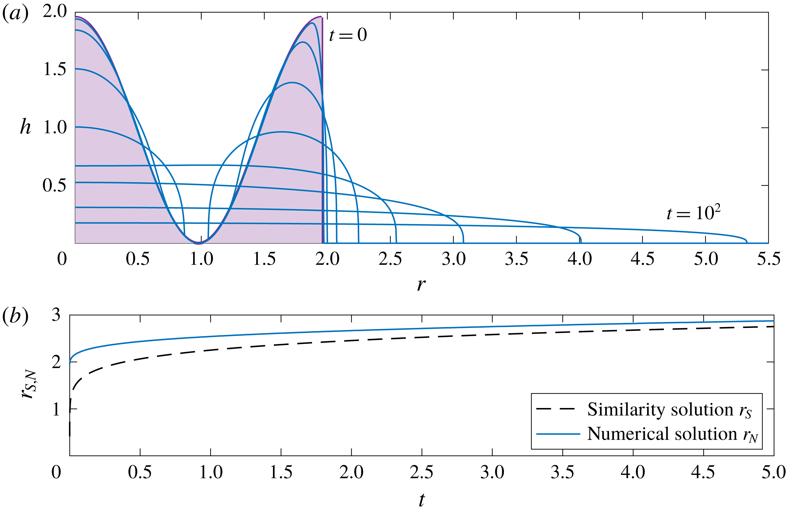
We also considered three ‘top hat’ initial profiles, denoted by ‘cylinder
 $J:1$
’, where
 $$\begin{eqnarray}\displaystyle r_{0} & = & \displaystyle J,\quad 0\leqslant h\leqslant 1/J,\end{eqnarray}$$
 $$\begin{eqnarray}\displaystyle & = & \displaystyle 1,\quad 1/J\leqslant h\leqslant 1,\end{eqnarray}$$
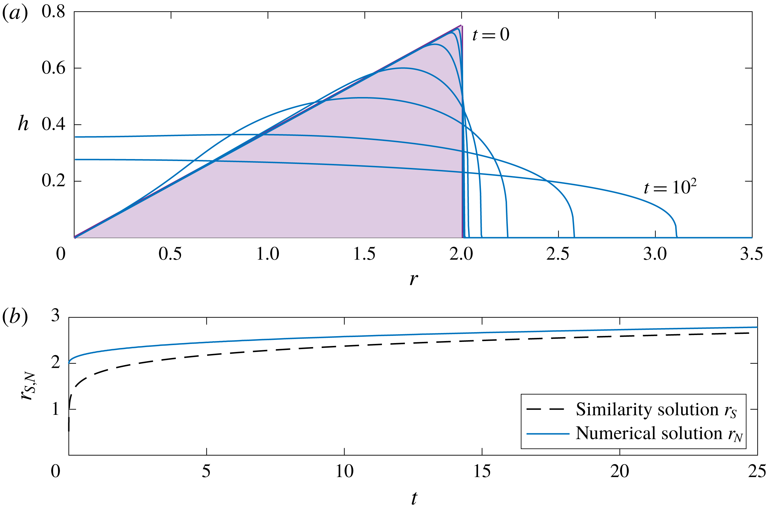
 $J=2,\,3$
and 5, as sketched in figure 6 for
 $J=2$
. The numerical integrations indicate that
 $$\begin{eqnarray}\displaystyle \unicode[STIX]{x1D6FD}V^{1/3}\unicode[STIX]{x1D6FE}_{0}^{8/3}\unicode[STIX]{x1D70F}\equiv \unicode[STIX]{x1D70F}^{\prime } & = & \displaystyle 4.90p^{-1}[1-0.020p+0(p^{2})]\quad (J=2),\end{eqnarray}$$
 $$\begin{eqnarray}\displaystyle & = & \displaystyle 16.3p^{-1}[1-0.021p+0(p^{2})]\quad (J=3),\end{eqnarray}$$
 $$\begin{eqnarray}\displaystyle & = & \displaystyle 79.6p^{-1}[1-0.022p+0(p^{2})]\quad (J=5),\end{eqnarray}$$
 $2.76p^{-1}[1-0.036p+0(p^{2})]$
for
 $J=1$
. Here, unlike the case for the cylinder there is choice about what values to take for the aspect ratio. We have taken
 $\unicode[STIX]{x1D6FE}_{0}=1/2$
,
 $1/3$
and
 $1/5$
for
 $J=2,3$
and 5 respectively.
(a) The shapes taken up by an initial ‘top hat’ profile with
 $\unicode[STIX]{x1D6FD}=1$
for
 $t=0$
,
 $10^{-4}$
,
 $10^{-3}$
,
 $10^{-2},\ldots ,10^{2}$
and (b) the curves of the radial extent as determined by the full numerical calculations (
 $r_{N}(t)$
; solid) and similarity solutions (
 $r_{S}(t)$
; dashed), respectively.

Numerically determined solutions as a function of
 $t$
for an inverse cone along with the values of
 $r_{N}(t)$
determined alongside
 $r_{S}(t)$
given by the similarity solution.

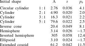
The constants
 $\unicode[STIX]{x1D700}$
and
 $A$
in the relationship
 $\unicode[STIX]{x1D70F}^{\prime }\equiv Ap^{-1}[1-\unicode[STIX]{x1D700}p+0(p^{2})]$
for various initial shapes and the corresponding maximum percentage divergence if the similarity solution is started at
 $t=t_{0}<0$
such that
 $r_{S}(0)=r_{N}(0)$
.

Numerically determined solutions as a function of
 $t$
for an extended cosoid along with the values of
 $r_{N}(t)$
determined alongside
 $r_{S}(t)$
given by the similarity solution.

For an inverse cone,
 $\unicode[STIX]{x1D70F}^{\prime }$
is given by
 $$\begin{eqnarray}\unicode[STIX]{x1D70F}^{\prime }=20.4p^{-1}[1-0.049p+0(p^{2})],\end{eqnarray}$$
as shown in figure 7.
The values that make up the right-hand side for various shapes is indicated in table 1 and further illustrated for the extended cosoid in figure 8. The relatively small values of
 $\unicode[STIX]{x1D700}$
indicate that the variation of
 $\unicode[STIX]{x1D70F}$
with
 $p$
is dominated by
 $\unicode[STIX]{x1D70F}\propto 1/p$
with the constant of proportionality dependent on the initial shape, and of course
 $(\unicode[STIX]{x1D6FD}V^{1/3}\unicode[STIX]{x1D6FE}_{0}^{8/3})^{-1}$
. Thus, to first order, at least, it takes ten times longer to attain 1 % accuracy than 10 %. Is this mainly
 $1/p$
dependence true for all such problems?
A different style of comparison is to consider the similarity solution initiated at
 $t=t_{0}<0$
, i.e. starting the similarity solution ‘early’ so the similarity and numerical solutions obey
 $r_{S}(0)=r_{N}(0)$
. The relative error is then zero (
 $p=0$
) initially, and returns to being proportional to
 $1/p$
for large times,
 $t\gg t_{0}$
. We thus expect only a range
 $0\leqslant |p|\leqslant |p_{0}|$
to be possible using this interpretation, where the sign of
 $p_{0}$
defines whether the numerical solution is greater (positive) or smaller (negative) than the adjusted similarity solution. A negative value of
 $p_{0}$
indicates that although they start together, the radius of the similarity solution always exceeds that of the numerical solution. Our eight investigated shapes yield
 $p_{0}$
values from
 $-$
1.7 to 11.5 as shown in table 1.
3 Some numerical values
(i) In the original experiments of Huppert (Reference Huppert1982),
 $\unicode[STIX]{x1D708}$
was either
 $13.2~\text{cm}^{2}~\text{s}^{-1}$
or, for one experiment,
 $1110~\text{cm}^{2}~\text{s}^{-1}$
, while
 $V$
lay between 220 and
 $933~\text{cm}^{3}$
. Thus, with
 $\unicode[STIX]{x0394}\unicode[STIX]{x1D70C}=\unicode[STIX]{x1D70C}$
because the density of the overlying air can be neglected,
 $\unicode[STIX]{x1D6FD}=24.8$
or
 $0.295~\text{cm}^{-1}~\text{s}^{-1}$
and
 $(\unicode[STIX]{x1D6FD}V^{1/3})^{-1}$
was between 0.004 s and 0.007 s except for the one experiment, with a high viscosity fluid, with
 $V=338~\text{cm}^{3}$
, for which it was 0.5 s, all very much less than the time taken to initiate the flow, by pouring fluid onto the surface or raising a container. Thus the approach to the similarity solution is on a time scale that is very rapid compared to the first reading at 10 s.
(ii) The original idea of Huppert’s work was to understand and analyse the data of the formation of the lava dome of the Soufrière of St. Vincent in 1979 (Huppert et al.
Reference Huppert, Shepherd, Sigurdsson and Sparks1982). They found that over a time of 100 days a volume of
 $41~\text{m}^{3}$
of lava was extruded (and
 $47~\text{m}^{3}$
over 150 days). From the data Huppert et al. determined that the viscosity of the lava was
 $2\times 10^{12}$
poise. Thus
 $\unicode[STIX]{x1D6FD}=1.5\times 10^{-7}~\text{m}^{-1}~\text{s}^{-1}$
and
 $V^{1/3}=3.45~\text{m}$
(over 100 days), leading to
 $(\unicode[STIX]{x1D6FD}V^{1/3})^{-1}\approx 10^{6}~\text{s}\sim 11$
days, suggesting that the lava dome had ample time to adjust to the similarity solution.
Actually, the data suggested that because of the gradual intrusion of magma into the lava dome
 $V=ct^{1.36}~\text{m}^{3}$
, where
 $c=0.0248~\text{m}^{3}~\text{s}^{-1.36}$
(and the data were fitted to a similarity solution for a volume increase like
 $t^{\unicode[STIX]{x1D6FC}}$
, where
 $\unicode[STIX]{x1D6FC}$
was determined from the data). In general, with
 $V=ct^{\unicode[STIX]{x1D6FC}}$
,
 $\unicode[STIX]{x1D6FD}$
and
 $c$
have dimensions
 $L^{-1}T^{-1}$
and
 $L^{3}T^{-\unicode[STIX]{x1D6FC}}$
respectively. Thus the only combination of
 $\unicode[STIX]{x1D6FD}$
and
 $c$
of dimensions
 $T$
is
 $(c\unicode[STIX]{x1D6FD}^{3})^{-1/(3+\unicode[STIX]{x1D6FC})}$
and so for the lava dome of St. Vincent,
 $\unicode[STIX]{x1D70F}\propto (c\unicode[STIX]{x1D6FD}^{3})^{-0.230}$
, which becomes
 $1.20\times 10^{5}s\sim 1.4$
days.
(iii) The shape of seven large volcanic lava domes on Venus were accurately measured during the Magellan expedition (McKenzie Reference McKenzie1992). Comparisons of the observed shape were made with: the Newtonian fluid model of Huppert (Reference Huppert1982); a Bingham fluid model incorporating a yield stress (Nye Reference Nye1952; Fink Reference Fink1987; Blake Reference Blake and Fink1990); and a model in which the spreading is controlled by the thin, highly viscous crust of the outer surface of the dome (Fink & Griffiths Reference Fink and Griffiths1990). The last was proposed because of numerous complaints about the model of Huppert (Reference Huppert1982), applied as described in the last subsection.
Nevertheless, McKenzie (Reference McKenzie1992) found clear evidence that Huppert’s model fitted the data very well; and the other two suggestions lead to poor fits. McKenzie’s results indicate that the viscosities of the different domes varied between
 $4.5\times 10^{14}$
and
 $1.0\times 10^{17}~\text{Pa}~\text{s}$
and their volumes between 176 and
 $1046~\text{km}^{3}$
. With
 $\unicode[STIX]{x1D70C}=3000~\text{kg}~\text{m}^{-3}$
,
 $g=8.87~\text{m}~\text{s}^{-2}$
,
 $\unicode[STIX]{x1D6FD}$
varies between
 $8.9\times 10^{-11}$
and
 $2.0\times 10^{-8}~\text{km}^{-1}~\text{s}^{-1}$
and
 $(\unicode[STIX]{x1D6FD}V^{1/3})^{-1}$
between 0.16 and 63 yr.
Alternatively, one of the very largest studied lava domes is Olympus Mons on Mars (diameter 625 km, height 25 km) with an area which could cover most of France, or the state of Arizona, for comparison. The values of the relevant parameters are
 $g=3.7~\text{ms}^{-2}$
,
 $\unicode[STIX]{x1D707}\sim 10^{4}~\text{Pa}~\text{s}$
,
 $\unicode[STIX]{x1D70C}=3000~\text{kgm}^{-3}$
and
 $V=4\times 10^{6}~\text{km}^{3}$
. Thus
 $\unicode[STIX]{x1D6FD}\sim 0.4~\text{km}^{-1}~\text{s}^{-1}$
and
 $(\unicode[STIX]{x1D6FD}V^{1/3})^{-1}\sim 10^{-1}~\text{s}$
, suggesting that the extrusion of Olympus Mons was well approximated by the similarity solution, in part because of its large volume.
4 The inverse problem
We have so far only considered direct problems – given a question, determine the answer. However, the analysis initiates a number of interesting inverse problems – given the answer, determine the initial conditions. The first is: what is the minimum number of
 $h(r,t)$
(or the cross-section of the current) to determine all the unknowns
 $g$
,
 $\unicode[STIX]{x0394}\unicode[STIX]{x1D70C}$
,
 $\unicode[STIX]{x1D708}$
,
 $V$
, initial shape,
 $r_{0}$
(
 $h_{0}$
then follows from
 $V$
and initial shape). The first part of the answer is that dynamic parameters
 $g$
,
 $\unicode[STIX]{x0394}\unicode[STIX]{x1D70C}$
and
 $\unicode[STIX]{x1D708}$
can never be determined individually; at best only the value of
 $\unicode[STIX]{x1D6FD}=g^{\prime }/3\unicode[STIX]{x1D708}$
. The second is whether
 $h(r,0+)$
is permissible, in which case
 $V$
, initial shape and
 $r_{0}$
are immediately known. Knowing in addition
 $r_{N}(t_{1})$
,
 $t_{1}\gg 0+$
, with the help of table 1 (possibly extended), one can evaluate
 $\unicode[STIX]{x1D6FD}$
. This would be done by evaluating
 $p_{1}=[r_{N}(t_{1})-r_{S}(t_{1})]/r_{S}(t_{1})$
, which with the appropriate form of (2.1) (for the determined initial shape), and with
 $\unicode[STIX]{x1D70F}=t_{1}$
, yields the value of
 $\unicode[STIX]{x1D6FD}$
.
If, alternatively, one is only given photos (i.e. cross-sections) for longish times
 $t$
, one can immediately evaluate
 $V$
, and the value of
 $\unicode[STIX]{x1D6FD}\unicode[STIX]{x1D6FE}_{0}^{8/3}/A$
, but no more. No matter how many (long time) profiles one has access to, nothing about the initial shape, or the value of
 $\unicode[STIX]{x1D6FD}$
, can be determined.
In summary, given photographs of the initial shape and some long time state of an experiment, one can determine all parameters (up to finding just
 $\unicode[STIX]{x1D6FD}$
). However, given as many late-time photographs as you desire, nothing can be determined about the initial shape or the value of
 $\unicode[STIX]{x1D6FD}$
.
5 Summary
We have shown that the time scale for any initial condition of volume
 $V$
to approach the similarity solution of (1.1) and (1.3) scales as
 $(\unicode[STIX]{x1D6FD}V^{1/3}\unicode[STIX]{x1D6FE}_{0}^{8/3})^{-1}$
, where
 $\unicode[STIX]{x1D6FE}_{0}$
is the initial ratio of height at the centre to radius, with variations in the premultiplicative constant dependent on the exact shape. Further, the time for approach is inversely proportional to the percentage difference between the radii of the current as determined by the full (nonlinear) solution and the similarity solution. Numerical calculations show that the time scale to equilibrate can vary between milliseconds in the laboratory to tens of years on Venus. The concepts put forward have several immediate generalisations, including: two-dimensional viscous gravity currents; axisymmetric and two-dimensional gravity currents in a porous medium; and high Reynolds number currents. Of course we have determined the time scales of solutions of (1.1), derived under the assumption of vanishingly small slopes, and (1.3), for arbitrary initial conditions. We have not determined the time scale for a real collapse which, especially for high initial aspect ratios, would lead to a quite different equation than (1.1). Indeed, the influence of vertical velocities would need to be incorporated and the governing equation would be more complicated. Nevertheless, we hypothesise that the time scales to approach the (small aspect ratio) similarity solutions are not very different.
Acknowledgements
We thank J. Lister, who wrote the numerical program on which our own program was based, and J. Chapman, C. Claret and G. Worster, with whom we have had a number of interesting conversations. During part of this work T.V.B. was supported by a grant from the James Bridgwater Trust, to which she, and H.E.H., are grateful. The paper answers a number of questions put to H.E.H. many times since 1982 by his good friend and close colleague, D. McKenzie. H.E.H. is grateful to Dan for his patience in being informed of the answers.
Appendix A. Straightforward extensions
The aim of this appendix is to derive rather simple extensions to the results obtained in the main body of the paper.
(i) Two-dimensional viscous gravity currents.
The governing equations for a two-dimensional gravity current of area
 $A$
propagating along the
 $x$
-axis from
 $x=0$
to
 $x=x_{N}(t)$
are (Huppert Reference Huppert1982)
 $$\begin{eqnarray}\displaystyle & h_{t}-\unicode[STIX]{x1D6FD}(h^{3}h_{x})_{x}=0, & \displaystyle\end{eqnarray}$$
 $$\begin{eqnarray}\displaystyle & \displaystyle \int _{0}^{x_{N}(t)}h\,\text{d}x=A. & \displaystyle\end{eqnarray}$$
Suitable similarity variables and solutions are given by
 $$\begin{eqnarray}\displaystyle & y=(\unicode[STIX]{x1D6FD}A^{3})^{-1/5}xt^{1/5}/\unicode[STIX]{x1D702}_{N}, & \displaystyle\end{eqnarray}$$
 $$\begin{eqnarray}\displaystyle & h(x,t)=(3/10)^{1/3}\unicode[STIX]{x1D702}_{N}^{2/3}(A^{2}/\unicode[STIX]{x1D6FD})^{1/5}t^{-1/5}(1-y^{2})^{1/3}, & \displaystyle\end{eqnarray}$$
 $$\begin{eqnarray}\displaystyle & x_{N}=\unicode[STIX]{x1D702}_{N}(\unicode[STIX]{x1D6FD}A^{3})^{1/5}t^{1/5}, & \displaystyle\end{eqnarray}$$
with
 $$\begin{eqnarray}\unicode[STIX]{x1D702}_{N}=[{\textstyle \frac{1}{5}}\left({\textstyle \frac{3}{10}}\right)^{1/3}\unicode[STIX]{x03C0}^{1/2}\unicode[STIX]{x1D6E4}(1/3)/\unicode[STIX]{x1D6E4}(5/6)]^{-3/5}=1.411\ldots .\end{eqnarray}$$
Thus
 $$\begin{eqnarray}\unicode[STIX]{x1D6FE}_{0}\equiv h(0,t)/x_{N}=(3/10)^{1/3}\unicode[STIX]{x1D702}_{N}^{-1/3}(\unicode[STIX]{x1D6FD}^{2}A^{2})^{-1/5},\end{eqnarray}$$
and the only time scale is
 $1/(\unicode[STIX]{x1D6FD}A^{1/2})$
.
If we now introduce new dimensionless variables via
 $$\begin{eqnarray}x=x_{0}X,\quad h=h_{0}H\quad \text{and}\quad t=T/(\unicode[STIX]{x1D6FD}A^{1/2}),\end{eqnarray}$$
(5.1) becomes
 $$\begin{eqnarray}H_{T}-\unicode[STIX]{x1D6FE}_{0}^{5/2}(H^{3}H_{x})_{x}=0.\end{eqnarray}$$
Thus, we suggest
 $$\begin{eqnarray}A^{1/2}\unicode[STIX]{x1D6FD}\unicode[STIX]{x1D70F}\unicode[STIX]{x1D6FE}_{0}^{5/2}=p^{-1}f_{a}(p,\text{shape}),\end{eqnarray}$$
where
 $f_{a}$
is a function of
 $p$
and the shape, but not dimensions, of the initial area of fluid.
(ii) Two-dimensional gravity currents in a porous medium.
The governing equations for a two-dimensional flow in a porous medium (Phillips Reference Phillips1991) with geometry as in (i) are
 $$\begin{eqnarray}h_{t}-\unicode[STIX]{x1D6FC}(hh_{x})_{x}=0,\end{eqnarray}$$
where
 $$\begin{eqnarray}\unicode[STIX]{x1D6FC}=k\unicode[STIX]{x0394}\unicode[STIX]{x1D70C}\unicode[STIX]{x1D6FE}/(\unicode[STIX]{x1D719}\unicode[STIX]{x1D707})\quad \text{or}\quad \unicode[STIX]{x0394}\unicode[STIX]{x1D70C}gb^{2}/(12\unicode[STIX]{x1D707}),\end{eqnarray}$$
with
 $k$
representing the permeability of the porous medium and
 $\unicode[STIX]{x1D719}$
the porosity in a flow often modelled in the laboratory as between two parallel plates apart a small distance
 $b$
, along with (A 2). A suitable similarity variable and solution for this combination are (Huppert & Woods Reference Huppert and Woods1995)
 $$\begin{eqnarray}\displaystyle & \unicode[STIX]{x1D709}=(9\unicode[STIX]{x1D6FC}A)^{-1/3}xt^{-1/3}, & \displaystyle\end{eqnarray}$$
 $$\begin{eqnarray}\displaystyle & h(x,t)=(9^{2/3}/6)(A^{2}/12)^{1/3}(1-\unicode[STIX]{x1D709}^{2})t^{-1/3}, & \displaystyle\end{eqnarray}$$
and
 $$\begin{eqnarray}x_{N}=(9\unicode[STIX]{x1D6FC}At)^{1/3}.\end{eqnarray}$$
Thus
 $$\begin{eqnarray}\unicode[STIX]{x1D6FE}_{0}\equiv h(l,t)/x_{N}=(9^{1/3}/6)(A/\unicode[STIX]{x1D6FC}^{2})^{1/3}t^{-2/3},\end{eqnarray}$$
and the only time scale is
 $A^{1/2}/\unicode[STIX]{x1D6FC}$
.
With (A 8) and
 $$\begin{eqnarray}t=A^{1/2}T/\unicode[STIX]{x1D6FC},\end{eqnarray}$$
equation (A 11) becomes
 $$\begin{eqnarray}H_{T}-\unicode[STIX]{x1D6FE}_{0}^{3/2}(HH_{X})_{X}=0,\end{eqnarray}$$
and therefore
 $$\begin{eqnarray}\unicode[STIX]{x1D6FC}A^{-1/2}\unicode[STIX]{x1D6FE}_{0}^{3/2}\unicode[STIX]{x1D70F}=p^{-1}f_{b}(p,\text{shape}).\end{eqnarray}$$
(iii) Axisymmetric gravity currents in a porous medium.
For this situation the governing equations are (Lyle et al. Reference Lyle, Huppert, Hallworth, Bickles and Chadwick2005)
 $$\begin{eqnarray}\displaystyle & h_{t}-{\displaystyle \frac{a}{r}}(rhh_{r})_{r}=0, & \displaystyle\end{eqnarray}$$
 $$\begin{eqnarray}\displaystyle & 2\unicode[STIX]{x03C0}\displaystyle \int _{0}^{r_{n}(t)}rh\,\text{d}r=V/\unicode[STIX]{x1D719}\equiv W, & \displaystyle\end{eqnarray}$$
(correcting an error in Lyle et al. (Reference Lyle, Huppert, Hallworth, Bickles and Chadwick2005), where
 $\unicode[STIX]{x1D719}$
was inadvertently omitted).
Appropriate similarity variable and solution are
 $$\begin{eqnarray}\displaystyle & z=(\unicode[STIX]{x1D6FC}W)^{-1/4}rt^{-1/4}/z_{N}, & \displaystyle\end{eqnarray}$$
 $$\begin{eqnarray}\displaystyle & \displaystyle h(r,t)=\frac{\unicode[STIX]{x03C0}}{2}^{-1/2}(W/\unicode[STIX]{x1D6FC})^{1/2}(1-z^{2})t^{-1/4}, & \displaystyle\end{eqnarray}$$
 $$\begin{eqnarray}\displaystyle & r_{N}=2(\unicode[STIX]{x1D6FC}W/\unicode[STIX]{x03C0})^{1/4}t^{1/4}. & \displaystyle\end{eqnarray}$$
Thus
 $$\begin{eqnarray}\unicode[STIX]{x1D6FE}_{0}\equiv h(0,t)/r_{N}={\textstyle \frac{1}{4}}(W/\unicode[STIX]{x03C0}\unicode[STIX]{x1D6FC}^{3})^{1/4}t^{-3/4},\end{eqnarray}$$
and the only time scale is
 $W^{1/3}/\unicode[STIX]{x1D6FC}$
.
Introducing
 $$\begin{eqnarray}r=r_{0}R,\quad h=h_{0}H\quad \text{and}\quad t=W^{1/3}T/\unicode[STIX]{x1D6FC}\end{eqnarray}$$
into (A 19), we determine that
 $$\begin{eqnarray}H_{r}-\frac{\unicode[STIX]{x1D6FE}_{0}}{R}^{4/3}(RHH_{R})_{R}=0,\end{eqnarray}$$
and it hence follows that
 $$\begin{eqnarray}\unicode[STIX]{x1D70F}=(W^{1/3}/\unicode[STIX]{x1D6FC})\unicode[STIX]{x1D6FE}_{0}^{-4/3}p^{-1}f_{c}(p,\text{shape}).\end{eqnarray}$$