1 Introduction
The existence of coherent structure in wall-bounded turbulence has been recognized for some time (Cantwell Reference Cantwell1981; Robinson Reference Robinson1991; Smits, McKeon & Marusic Reference Smits, McKeon and Marusic2011). In more recent years there has been increasing interest in large-scale coherent features, particularly at high Reynolds numbers (Kim & Adrian Reference Kim and Adrian1999; Adrian, Meinhart & Tomkins Reference Adrian, Meinhart and Tomkins2000; Guala, Hommema & Adrian Reference Guala, Hommema and Adrian2006; Balakumar & Adrian Reference Balakumar and Adrian2007; Hutchins & Marusic Reference Hutchins and Marusic2007a ; Monty et al. Reference Monty, Stewart, Williams and Chong2007; Jiménez Reference Jiménez2012). These large-scale structures contribute significantly to the turbulent kinetic energy and the Reynolds stresses in the outer region (Komminaho, Lundbladh & Johansson Reference Komminaho, Lundbladh and Johansson1996; Tomkins & Adrian Reference Tomkins and Adrian2005; Guala et al. Reference Guala, Hommema and Adrian2006). Furthermore there is evidence that their presence is felt near the wall through a modulation of the near-wall cycle (Abe, Kawamura & Choi Reference Abe, Kawamura and Choi2004; Hutchins & Marusic Reference Hutchins and Marusic2007b ; Mathis, Hutchins & Marusic Reference Mathis, Hutchins and Marusic2009). The importance of these large-scale structures is therefore clear and motivates efforts towards their estimation and control.
Meanwhile, in what started as a separate community, analysis of the linearized Navier–Stokes equations has allowed (amongst other things) structure in shear flows to be elucidated. In the earliest studies this analysis was performed for laminar shear flows by considering the temporal development of small perturbations about the laminar flow. Of particular significance was the realization that, even for stable flows, perturbations can experience significant transient growth before ultimately decaying (Gustavsson Reference Gustavsson1991; Schmid & Henningson Reference Schmid and Henningson2001). This transient amplification is explained by the non-normality of the Navier–Stokes equations in the presence of shear (Trefethen et al. Reference Trefethen, Trefethen, Reddy and Driscoll1993; Farrell & Ioannou Reference Farrell and Ioannou1996). Related studies are typically concerned with finding the initial condition leading to the largest possible transient growth – that is, an initial value problem – which has been performed across a number of canonical laminar shear flows (Butler & Farrell Reference Butler and Farrell1992; Reddy & Henningson Reference Reddy and Henningson1993; Schmid & Henningson Reference Schmid and Henningson1994; Andersson, Berggren & Henningson Reference Andersson, Berggren and Henningson1999). An alternative approach has been to take an input–output point of view by looking at the response of the linearized Navier–Stokes equations to an impulse (Jovanovic & Bamieh Reference Jovanovic and Bamieh2001; Jovanovic Reference Jovanovic2004); to stochastic forcing (Farrell & Ioannou Reference Farrell and Ioannou1993; Bamieh & Dahleh Reference Bamieh and Dahleh2001; Jovanovic & Bamieh Reference Jovanovic and Bamieh2005); and to harmonic forcing (Jovanovic Reference Jovanovic2004; Schmid Reference Schmid2007).
Linear analysis for fully developed turbulent shear flow – although able to claim a relatively long history (Malkus Reference Malkus1956; Reynolds & Tiederman Reference Reynolds and Tiederman1967; Reynolds & Hussain Reference Reynolds and Hussain1972) – has to date received less attention than its laminar counterpart. In recent years, however, there has been a renewed interest in linear models for turbulent shear flows, spurred on in part by mounting evidence that linear mechanisms play an important role even here. In a manner analogous to the laminar case, the linearized Navier–Stokes equations (now linearized about the mean flow) have been studied in a transient growth setting (del Álamo & Jiménez Reference del Álamo and Jiménez2006; Cossu, Pujals & Depardon Reference Cossu, Pujals and Depardon2009; Pujals et al. Reference Pujals, García-Villalba, Cossu and Depardon2009) and in an input–output setting (Hwang & Cossu Reference Hwang and Cossu2010a ,Reference Hwang and Cossu b ; Willis, Hwang & Cossu Reference Willis, Hwang and Cossu2010). All of these studies follow the early work of Reynolds & Tiederman (Reference Reynolds and Tiederman1967) by augmenting the kinematic viscosity with an eddy viscosity to model the effect of the smallest scales on the large, coherent motions of interest.
In related but separate work, linear mechanisms in fully developed turbulent shear flows have also been studied in recent years using a resolvent-based approach (McKeon & Sharma Reference McKeon and Sharma2010; McKeon, Sharma & Jacobi Reference McKeon, Sharma and Jacobi2013). This approach proceeds by essentially performing a Reynolds decomposition of the Navier–Stokes equations and then, in a novel development, treating any terms nonlinear in the perturbations as unknown forcings to an otherwise linear system. The decomposition is exact and thus no linearization is performed. Put another way, no terms are discarded, the nonlinear terms instead being absorbed into the unknown forcing. A resolvent analysis is then used to extract structure in the linear operator. Importantly, the analysis is able to reproduce pertinent features of fully developed turbulent shear flows (Moarref et al. Reference Moarref, Sharma, Tropp and McKeon2013, Reference Moarref, Jovanović, Tropp, Sharma and McKeon2014; Sharma & McKeon Reference Sharma and McKeon2013).
This paper investigates model-based estimation of channel flow at a friction Reynolds number of
 $Re_{\unicode[STIX]{x1D70F}}=1000$
. To do so we use the linear modelling approach of McKeon & Sharma (Reference McKeon and Sharma2010) (described in § 2) by treating any nonlinear terms as unknown forcings to an otherwise linear system. We will see in § 3 that this point of view can be naturally framed as an optimal linear estimation problem. While following closely the development of McKeon & Sharma (Reference McKeon and Sharma2010), the work also shares similarities with a number of other previous studies (Bamieh & Dahleh Reference Bamieh and Dahleh2001; Jovanovic & Bamieh Reference Jovanovic and Bamieh2005; Zare, Jovanovic & Georgiou Reference Zare, Jovanovic and Georgiou2017). What all of these studies share in common is that they all focus on the linear dynamics of the Navier–Stokes equations; and that they all do so using an input–output point of view. The estimator uses time-resolved velocity information at a single wall-normal location to estimate the velocity field at other wall-normal locations. (The data coming from direct numerical simulations.) We focus specifically on estimating the largest scales. This is motivated not only by their importance at high Reynolds numbers as described above, but also by our expectation that they are the scales that will show the greatest coherence across wall-normal locations, and therefore represent the most promising candidates for any estimation scheme. We will see that, for these largest scales, the estimator performance is improved by including an eddy viscosity in the linear operator.
Linear estimation has been applied to wall-bounded flows at laminar Reynolds numbers (Hœpffner et al. Reference Hœpffner, Chevalier, Bewley and Henningson2005; Jones et al. Reference Jones, Kerrigan, Morrison and Zaki2011) and at very low turbulent Reynolds numbers (Chevalier et al. Reference Chevalier, Hœpffner, Bewley and Henningson2006). The contribution of this work is to apply similar tools to fully developed turbulence at a relatively high Reynolds number. The work is important and timely for two reasons. First for modelling: if a linear estimation scheme succeeds, then this is further evidence of the importance of linear mechanisms. More specifically if the largest scales are well estimated by a linear model, then this provides compelling evidence that they are driven at least in part by a linear mechanism. Second, for flow estimation and control: success with a linear model alone – the tools for which are well developed – would bode well for the estimation and control of large-scale structures in turbulent shear flows at high Reynolds numbers.
2 Linear model
We consider fully developed turbulent flow in a channel at
 $Re_{\unicode[STIX]{x1D70F}}=1000$
. The streamwise, spanwise and wall-normal directions are denoted by
 $x$
,
 $y$
and
 $z$
; and the corresponding velocity components by
 $u$
,
 $v$
and
 $w$
. The Reynolds number
 $Re_{\unicode[STIX]{x1D70F}}$
is based on the channel half-height
 $h$
, kinematic viscosity
 $\unicode[STIX]{x1D708}$
and friction velocity
 $u_{\unicode[STIX]{x1D70F}}=\sqrt{\unicode[STIX]{x1D70F}_{w}/\unicode[STIX]{x1D70C}}$
, where
 $\unicode[STIX]{x1D70F}_{w}$
is the wall shear stress and
 $\unicode[STIX]{x1D70C}$
is the density. Thus velocities are normalized by
 $u_{\unicode[STIX]{x1D70F}}$
; spatial variables by
 $h$
; time by
 $h/u_{\unicode[STIX]{x1D70F}}$
; and pressure by
 $\unicode[STIX]{x1D70C}u_{\unicode[STIX]{x1D70F}}^{2}$
. Following this non-dimensionalization, the channel half-height is unity so that
 $z\in [0,2]$
. We will use this non-dimensionalization throughout, meaning (for example) that
 $u$
can be taken to mean
 $\tilde{u} /u_{\unicode[STIX]{x1D70F}}$
(where
 $\tilde{u}$
is dimensional);
 $(k_{x},k_{y})$
(the streamwise and spanwise wavenumbers) can be taken to mean
 $(\tilde{k}_{x}h,\tilde{k}_{y}h)$
;
 $(\unicode[STIX]{x1D706}_{x},\unicode[STIX]{x1D706}_{y})$
(the streamwise and spanwise wavelengths) can be taken to mean
 $(\tilde{\unicode[STIX]{x1D706}}_{x}/h,\tilde{\unicode[STIX]{x1D706}}_{y}/h)$
; and so on. Spatial variables will receive a
 $+$
superscript when normalized by the viscous length scale, e.g.
 $z^{+}=\tilde{z}u_{\unicode[STIX]{x1D70F}}/\unicode[STIX]{x1D708}$
.
The linear model is obtained by performing a Reynolds decomposition of the velocity field; substituting this into the non-dimensional Navier–Stokes equations; and subtracting the mean equations to arrive at
 $$\begin{eqnarray}\frac{\unicode[STIX]{x2202}\boldsymbol{u}}{\unicode[STIX]{x2202}t}=-(\boldsymbol{U}\boldsymbol{\cdot }\unicode[STIX]{x1D735})\boldsymbol{u}-(\boldsymbol{u}\boldsymbol{\cdot }\unicode[STIX]{x1D735})\boldsymbol{U}-\unicode[STIX]{x1D735}p+Re_{\unicode[STIX]{x1D70F}}^{-1}\unicode[STIX]{x1D6FB}^{2}\boldsymbol{u}+\boldsymbol{d},\quad \unicode[STIX]{x1D735}\boldsymbol{\cdot }\boldsymbol{u}=0,\end{eqnarray}$$
where
 $\boldsymbol{U}$
is the mean velocity profile and
 $\boldsymbol{u}$
represents turbulent fluctuations about the mean. Following McKeon & Sharma (Reference McKeon and Sharma2010), any nonlinear terms in (2.1) are treated as a forcing
 $\boldsymbol{d}$
to an otherwise linear system, the forcing given by
 $\boldsymbol{d}=-(\boldsymbol{u}\boldsymbol{\cdot }\unicode[STIX]{x1D735})\boldsymbol{u}+\overline{(\boldsymbol{u}\boldsymbol{\cdot }\unicode[STIX]{x1D735})\boldsymbol{u}}$
. Nonlinear effects thus manifest themselves in two ways: through their role in setting the mean velocity profile
 $\boldsymbol{U}$
; and through their forcing of the linear operator.
For the mean velocity profile
 $\boldsymbol{U}=(U(z),0,0)$
we use the Cess (Reference Cess1958) approximation for the turbulent eddy viscosity (Reynolds & Hussain Reference Reynolds and Hussain1972):
 $$\begin{eqnarray}\unicode[STIX]{x1D708}_{T}(z)=\frac{\unicode[STIX]{x1D708}}{2}\left(1+\frac{\unicode[STIX]{x1D705}^{2}Re_{\unicode[STIX]{x1D70F}}^{2}}{9}(2z-z^{2})^{2}(3-4z+z^{2})^{2}\left[1-\exp \left(\frac{-Re_{\unicode[STIX]{x1D70F}}z}{A}\right)\right]^{2}\right)^{1/2}+\frac{\unicode[STIX]{x1D708}}{2},\end{eqnarray}$$
where
 $\unicode[STIX]{x1D708}_{T}(z)$
is the total viscosity (i.e. including the kinematic viscosity). As in previous studies we take
 $\unicode[STIX]{x1D705}=0.426$
and
 $A=25.4$
, which we note were optimized for
 $Re_{\unicode[STIX]{x1D70F}}=2003$
(del Álamo & Jiménez Reference del Álamo and Jiménez2006; Pujals et al.
Reference Pujals, García-Villalba, Cossu and Depardon2009; Moarref et al.
Reference Moarref, Sharma, Tropp and McKeon2013). The mean velocity profile
 $\boldsymbol{U}$
is then given by integrating
 $Re_{\unicode[STIX]{x1D70F}}(1-z)\unicode[STIX]{x1D708}/\unicode[STIX]{x1D708}_{T}(z)$
.
2.1 State-space description
We now want to bring the linear model (2.1) into state-space form – doing so will allow us to use standard tools from dynamics and control to design an estimator in § 3. This is achieved by taking Fourier transforms in the homogeneous directions (
 $x$
,
 $y$
); transforming into Orr–Sommerfeld Squire form; and discretizing in the wall-normal direction (
 $z$
) using Chebyshev collocation. In this way we arrive at a state-space model governing the wall-normal velocity
 $\hat{\boldsymbol{w}}$
and the wall-normal vorticity
 $\hat{\boldsymbol{\unicode[STIX]{x1D702}}}$
in Fourier space at a single wavenumber pair (
 $k_{x}$
,
 $k_{y}$
):
 $$\begin{eqnarray}\displaystyle & \displaystyle \dot{\boldsymbol{x}}(t)=\unicode[STIX]{x1D63C}\boldsymbol{x}(t)+\unicode[STIX]{x1D63D}\boldsymbol{d}(t), & \displaystyle\end{eqnarray}$$
 $$\begin{eqnarray}\displaystyle & \displaystyle \boldsymbol{y}(t)=\unicode[STIX]{x1D63E}\boldsymbol{x}(t), & \displaystyle\end{eqnarray}$$
 $\boldsymbol{x}=\left[\begin{array}{@{}c@{}}\hat{\boldsymbol{w}}~\hat{\boldsymbol{\unicode[STIX]{x1D702}}}\end{array}\right]^{\text{T}}$
;
 $\boldsymbol{y}=\left[\begin{array}{@{}c@{}}\hat{\boldsymbol{u}}~\hat{\boldsymbol{v}}~\hat{\boldsymbol{w}}\end{array}\right]^{\text{T}}$
; and
 $\boldsymbol{d}=\left[\begin{array}{@{}c@{}}\hat{\boldsymbol{d}}_{x}~\hat{\boldsymbol{d}}_{y}~\hat{\boldsymbol{d}}_{z}\end{array}\right]^{\text{T}}$
represents all nonlinear terms (see (2.1)), which we treat as an unknown disturbance in all of the following. The matrices
 $\unicode[STIX]{x1D63C}$
,
 $\unicode[STIX]{x1D63D}$
and
 $\unicode[STIX]{x1D63E}$
are defined in appendix A. Equation (2.3) is in standard state-space form, which we will now use for estimator design.
3 Linear estimation
Our ultimate goal is to use limited measurements to estimate a fluid flow at other locations. A common way to do this in the fluid mechanics community is to use linear stochastic estimation (Adrian & Moin Reference Adrian and Moin1988). Here we take a different approach by using the linear models just described, together with tools from optimal control, to design an optimal estimator. (We will define in what sense it is optimal in the following.)
Consider a linear state-space model of the form
 $$\begin{eqnarray}\displaystyle & \displaystyle \dot{\boldsymbol{x}}(t)=\unicode[STIX]{x1D63C}\boldsymbol{x}(t)+\unicode[STIX]{x1D63D}\boldsymbol{d}(t), & \displaystyle\end{eqnarray}$$
 $$\begin{eqnarray}\displaystyle & \displaystyle \boldsymbol{y}(t)=\unicode[STIX]{x1D63E}_{y}\boldsymbol{x}(t)+\boldsymbol{n}(t), & \displaystyle\end{eqnarray}$$
 $$\begin{eqnarray}\displaystyle & \displaystyle \boldsymbol{z}(t)=\unicode[STIX]{x1D63E}_{z}\boldsymbol{x}(t), & \displaystyle\end{eqnarray}$$
 $\boldsymbol{y}$
and the quantities to be estimated
 $\boldsymbol{z}$
. (Each of these can be written as a linear combination of the state
 $x$
using matrices
 $\unicode[STIX]{x1D63E}_{y}$
and
 $\unicode[STIX]{x1D63E}_{z}$
, as described in more detail in appendix A.) Second, the measurements
 $\boldsymbol{y}$
are contaminated by sensor noise
 $\boldsymbol{n}$
. If the state-space model (3.1) has
 $n$
states,
 $p$
disturbances,
 $q$
measurements and
 $r$
estimated quantities, then the state-space matrices have the following dimensions:
 $\unicode[STIX]{x1D63C}\in \mathbb{C}^{n\times n}$
;
 $\unicode[STIX]{x1D63D}\in \mathbb{C}^{n\times p}$
;
 $\unicode[STIX]{x1D63E}_{y}\in \mathbb{C}^{q\times n}$
; and
 $\unicode[STIX]{x1D63E}_{z}\in \mathbb{C}^{r\times n}$
.
Thus there are two unknown exogenous inputs in (3.1). The first is sensor noise,
 $\boldsymbol{n}$
, which contaminates measurements so that the measured value,
 $\boldsymbol{y}$
, differs from the true value. The second is disturbances
 $\boldsymbol{d}$
that, by their nature, are unknown. (In the present case these correspond to the terms quadratic in
 $\boldsymbol{u}$
– see § 2.) Taking Laplace transforms of (3.1), setting
 $\boldsymbol{n}=0$
(for the moment), and rearranging, we arrive at the transfer function
 $\unicode[STIX]{x1D64B}(s)$
, defined such that
 $\left[\begin{array}{@{}c@{}}\boldsymbol{z}(s)~\boldsymbol{y}(s)\end{array}\right]^{\text{T}}=\unicode[STIX]{x1D64B}(s)\boldsymbol{d}(s)$
:
 $$\begin{eqnarray}\unicode[STIX]{x1D64B}(s)=\left[\begin{array}{@{}c@{}}\unicode[STIX]{x1D64B}_{z}(s)\\ \unicode[STIX]{x1D64B}_{y}(s)\end{array}\right]=\left[\begin{array}{@{}c@{}}\unicode[STIX]{x1D63E}_{z}\\ \unicode[STIX]{x1D63E}_{y}\end{array}\right](s\unicode[STIX]{x1D644}-\unicode[STIX]{x1D63C})^{-1}\unicode[STIX]{x1D63D},\end{eqnarray}$$
where
 $s$
is the Laplace variable. We note in passing that, by setting
 $s=\text{i}\unicode[STIX]{x1D714}$
, we recover the frequency response – more commonly referred to as the resolvent – from the unknown forcing
 $\boldsymbol{d}$
to the velocity field at the estimation (
 $\boldsymbol{z}$
) and measurement (
 $\boldsymbol{y}$
) locations.
Having defined the relevant transfer functions, we can now consider the overall block diagram for the estimation problem:

In general the transfer function
 $\unicode[STIX]{x1D64B}(s)$
is weighted (the reasons for which are given in appendix B), but here we instead use the unweighted
 $\unicode[STIX]{x1D64B}(s)$
to simplify the discussion. The weighted plant is introduced as part of the more detailed description given in appendix B. The estimator
 $\unicode[STIX]{x1D641}(s)$
(to be designed) receives as its input the measured quantities
 $\boldsymbol{y}$
(contaminated by noise
 $\boldsymbol{n}$
), and provides as its output an estimate of the quantities of interest
 $\boldsymbol{z}$
. We label this estimate
 $\boldsymbol{z}_{e}$
. The estimation error
 $\boldsymbol{e}$
is then
 $\boldsymbol{e}=\boldsymbol{z}-\boldsymbol{z}_{e}.$
We can now define an overall transfer function
 $\unicode[STIX]{x1D642}(s)$
, as indicated by the dashed box in (3.3).
 $\unicode[STIX]{x1D642}$
receives as its input the unknown disturbances
 $\boldsymbol{d}$
and the sensor noise
 $\boldsymbol{n}$
; and provides as its output the estimation error
 $\boldsymbol{e}$
.
 $\unicode[STIX]{x1D642}(s)$
is thus defined such that its input is the unknown (and unwanted) exogenous inputs; and its output is the quantity that we want to keep small (the estimation error). The estimation problem can now be stated as follows: given
 $\unicode[STIX]{x1D64B}$
, design
 $\unicode[STIX]{x1D641}$
such that
 $\unicode[STIX]{x1D642}$
is small. If this is achieved then the estimation error should remain small even in the presence of the unknown disturbances
 $\boldsymbol{d}$
and sensor noise
 $\boldsymbol{n}$
.
In order to design the filter
 $\unicode[STIX]{x1D641}$
we must first define a suitable measure of the size of
 $\unicode[STIX]{x1D642}$
. For this we use the 2-norm, defined for a transfer function as
 $$\begin{eqnarray}\Vert \unicode[STIX]{x1D642}\Vert _{2}=\sqrt{\frac{1}{2\unicode[STIX]{x03C0}}\int _{-\infty }^{\infty }\text{Trace}[\unicode[STIX]{x1D642}^{\ast }(\text{i}\unicode[STIX]{x1D714})\unicode[STIX]{x1D642}(\text{i}\unicode[STIX]{x1D714})]\,\text{d}\unicode[STIX]{x1D714}}=\sqrt{\frac{1}{2\unicode[STIX]{x03C0}}\int _{-\infty }^{\infty }\mathop{\sum }_{i}\unicode[STIX]{x1D70E}_{i}^{2}(\text{i}\unicode[STIX]{x1D714})\,\text{d}\unicode[STIX]{x1D714}},\end{eqnarray}$$
where
 $\unicode[STIX]{x1D70E}_{i}(\text{i}\unicode[STIX]{x1D714})$
are the singular values of
 $\unicode[STIX]{x1D642}$
at frequency
 $\unicode[STIX]{x1D714}$
and represent a generalization of gain when there are many inputs and many outputs. The 2-norm therefore represents an average gain over all frequencies and all directions and it is this quantity that is minimized in the filter design. (More specifically, the 2-norm in (3.4) is defined such that it corresponds to a grid-independent energy-norm.)
 $\unicode[STIX]{x1D641}$
can now be formed using standard tools by first transforming the block diagram (3.3) into a more standard form as described in appendix B.
One final remark. A common way to design the filter described in this section is to use Kalman filtering. The framework chosen here is often referred to as
 ${\mathcal{H}}_{2}$
control, of which Kalman filtering is a special case. We have chosen this framework – despite the fact that it is less standard – because it is both more intuitive and more general. For more on estimator design in this setting see Seron, Braslavsky and Goodwin (Reference Seron, Braslavsky and Goodwin2012).
4 DNS dataset
We require two sets of time-resolved velocity data: (i) the velocity field in the measurement plane(s) which serves as the input for the linear estimator; and (ii) the velocity field in the estimation plane(s) so that we can compare the estimate with the truth. These data are taken from the Johns Hopkins Turbulence Database (Graham et al.
Reference Graham, Kanov, Yang, Lee, Malaya, Lalescu, Burns, Eyink, Szalay, Moser and Meneveau2016). The direct numerical simulations (DNS) are performed in a channel of size
 $8\unicode[STIX]{x03C0}\times 3\unicode[STIX]{x03C0}\times 2$
using
 $2048\times 1536\times 512$
nodes. The simulations solve the incompressible Navier–Stokes equations using the pseudo-spectral (Fourier–Galerkin) method in the wall-parallel planes and the seventh-order B-spline collocation method in the wall-normal direction.
4.1 Spatial resolution
The smallest non-zero wavenumbers resolved are
 $|k_{x}|=1/4$
in the streamwise direction and
 $|k_{y}|=2/3$
in the spanwise direction. The largest wavenumbers resolved are
 $|k_{x}|=256$
and
 $|k_{y}|=512$
. Since our interest is in estimating the largest structures, only wavenumbers satisfying
 $|k_{x}|\leqslant 8$
,
 $|k_{y}|\leqslant 64/3$
will be included – for both the DNS data and the linear estimator – in the results to follow in § 5. This corresponds to
 $\unicode[STIX]{x1D706}_{x}\geqslant 0.785$
and
 $\unicode[STIX]{x1D706}_{y}\geqslant 0.295$
(recall that the channel half-height is unity) or
 $\unicode[STIX]{x1D706}_{x}^{+}\geqslant 785$
and
 $\unicode[STIX]{x1D706}_{y}^{+}\geqslant 295$
. We will see in the results to follow that these are sensible choices.
4.2 Temporal resolution
Time-resolved data are available for approximately one channel flow-through time (
 $t_{max}U_{c}/8\unicode[STIX]{x03C0}=1.15$
, where
 $U_{c}$
is the mean velocity at the channel centre). While this means that some results are not fully converged, we will see in § 5 that it is sufficient to characterize the performance of the linear estimators. Data have been acquired at a temporal resolution of
 $\unicode[STIX]{x0394}t=0.0016$
(
 $\unicode[STIX]{x0394}tU_{c}=0.0362$
;
 $\unicode[STIX]{x0394}t^{+}=1.60$
). This corresponds to every twenty-fifth DNS time step. It is important that the time step is small enough to resolve the frequencies of interest at a given (
 $k_{x}$
,
 $k_{y}$
) pair. This can be checked using Taylor’s hypothesis. If Taylor’s hypothesis is approximately true, then a structure with streamwise wavenumber
 $k_{x}$
measured at a wall-normal height
 $z$
will give rise to a temporal frequency
 $\unicode[STIX]{x1D714}=k_{x}U(z)$
as it convects downstream. The highest frequency that we anticipate will therefore be for the largest streamwise wavenumber (
 $|k_{x}|=8$
) and the largest mean velocity (
 $U(z^{+}=297)=19.3$
) to give a maximum frequency of
 $|\unicode[STIX]{x1D714}|=154.4$
. We therefore have access to approximately 25 samples per period for this highest frequency.
5 Results
We now apply the model-based estimator described in § 3 to the channel flow DNS described in § 4. Recall that the models (and therefore estimators) are formed in Fourier space at a given (
 $k_{x}$
,
 $k_{y}$
) pair. The wavenumber spacing (
 $\unicode[STIX]{x0394}k_{x}=1/4$
,
 $\unicode[STIX]{x0394}k_{y}=2/3$
) and the maximum wavenumbers considered (
 $|k_{x}|=8$
,
 $|k_{y}|=64/3$
) make for
 $65\times 65=4225$
wavenumber pairs in total. However, the real-valued data (in physical space) mean that the results for (
 $+k_{x}$
,
 $-k_{y}$
) are equivalent to those for (
 $+k_{x}$
,
 $+k_{y}$
), and so we only need consider non-negative spanwise wavenumbers
 $k_{y}\geqslant 0$
. (Alternatively we could choose to include only non-negative streamwise wavenumbers,
 $k_{x}\geqslant 0$
, provided that both positive and negative spanwise wavenumbers are included.) This makes for
 $65\times 33=2145$
wavenumber pairs. In the wall-normal direction we use 151 Chebyshev points, which is sufficient for the large scales of interest. Convergence has been checked by doubling the number of Chebyshev points and ensuring that the results do not change.
5.1 Choice of measurement quantity
In all results to follow, the quantities measured (
 $\boldsymbol{y}$
in (3.3)) are all three velocity components at
 $z^{+}=197$
. These measurements are clearly not as practical as a wall-based measurement scheme; and furthermore, the exact choice of wall-normal location may seem arbitrary. Therefore we first discuss and justify this choice before moving on to the results obtained with it.
First concerning practicality: it would be more practical, of course, to measure some wall-based quantity such as wall pressure or wall shear stress. But we argue that, rather than jump straight to what is practical, it is more instructive in the present case to start with something that is not practical but which is more direct (in the sense that the quantity measured is a velocity, and the quantity estimated is also a velocity). Indeed, suppose that we measure instead the wall shear stress – and use it to estimate the velocity at some wall height – and suppose that we do not succeed. What can we conclude? Is it because the linear model used for estimation is not suitable; or is it because there is not enough coherence between what is measured (the wall shear stress) and what is estimated (the velocity at some wall height)? In other words, with more than one obstacle to success, it is difficult to isolate the one responsible for failure. In this study we would therefore like to minimize the obstacles to failure (at the cost of practicality) in order to make success with a linear model as likely as it can be.
Having justified our choice of velocity as measurement, it remains to justify the specific choice of wall height (at
 $z^{+}=197$
). This choice is based primarily on the work of Hwang & Cossu (Reference Hwang and Cossu2010b
), who find that the optimally amplified structures in fully developed turbulent channel flow take the form of streamwise streaks. Significantly for the present work, they also find that the streamwise velocity component of these structures reaches its peak value at a wall height of approximately
 $0.2h$
from either wall, corresponding to
 $z^{+}=200$
in the present case. The measurement location of
 $z^{+}=197$
thus corresponds approximately to the wall height where the large-scale structures (that we would like to estimate) are most energetic.
5.2 Estimator performance in physical space
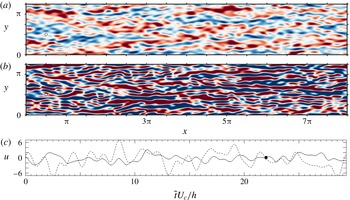
We now look at the linear estimator’s performance in physical space. This is shown in figure 1 where the estimate of the streamwise velocity perturbation at
 $z^{+}=101$
is compared to the true (i.e. DNS) value at a single instant in time. (Movies of the estimator performance are also provided at both
 $z^{+}=101$
and
 $z^{+}=297$
.) We also plot the time history of the streamwise velocity perturbation at a single point in the plane. We make two observations on the results seen in figure 1. First, that the linear estimator tends to overpredict the amplitude of the streamwise velocity perturbations. Second, that this overprediction appears to be concentrated in structures that are long in the streamwise direction and thin in the spanwise direction. We will investigate this tendency more thoroughly in § 5.4 by moving into Fourier space. Before doing so, however, we will first repeat the results of figure 1 using an alternative linear model which includes in it a simple eddy viscosity model.
Estimation of the streamwise velocity perturbation at
 $z^{+}=101$
using the linear model (2.1): (a) DNS data; and (b) linear estimate using measurements at
 $z^{+}=197$
; (c) time history at
 $x=\unicode[STIX]{x03C0}/2$
,
 $y=\unicode[STIX]{x03C0}/2$
for the DNS data (——) and for the linear estimate (– –). Sixty-five contour levels are shown from
 $u=-3.5$
(blue) to
 $u=+3.5$
(red). Movies of the estimator performance are also provided at both
 $z^{+}=101$
and
 $z^{+}=297$
.

5.3 Including an eddy viscosity in the linear operator
An alternative linear model can be formed by first performing a triple decomposition of the velocity field,
 $\tilde{\boldsymbol{u}}=\boldsymbol{U}+\boldsymbol{u}+\boldsymbol{u}^{\prime }$
, where
 $\boldsymbol{U}$
is again the mean velocity;
 $\boldsymbol{u}$
represents a large-scale organized motion; and
 $\boldsymbol{u}^{\prime }$
represents small-scale turbulent fluctuations. Following previous work (Reynolds & Hussain Reference Reynolds and Hussain1972; del Álamo & Jiménez Reference del Álamo and Jiménez2006; Pujals et al.
Reference Pujals, García-Villalba, Cossu and Depardon2009; Hwang Reference Hwang2016) we provide a closure for terms quadratic in
 $\boldsymbol{u}^{\prime }$
using a simple eddy viscosity model. In contrast to these previous studies, however, we retain terms quadratic in
 $\boldsymbol{u}$
and treat them as unknown forcings as we did for (2.1). In this way we obtain a linear model, augmented by an eddy viscosity, and forced by the remaining nonlinear terms:
 $$\begin{eqnarray}\frac{\unicode[STIX]{x2202}\boldsymbol{u}}{\unicode[STIX]{x2202}t}=-(\boldsymbol{U}\boldsymbol{\cdot }\unicode[STIX]{x1D735})\boldsymbol{u}-(\boldsymbol{u}\boldsymbol{\cdot }\unicode[STIX]{x1D735})\boldsymbol{U}-\unicode[STIX]{x1D735}p+\unicode[STIX]{x1D735}\boldsymbol{\cdot }\left[\frac{\unicode[STIX]{x1D708}_{T}}{\unicode[STIX]{x1D708}}(\unicode[STIX]{x1D735}\boldsymbol{u}+\unicode[STIX]{x1D735}\boldsymbol{u}^{\text{T}})\right]+\boldsymbol{d},\quad \unicode[STIX]{x1D735}\boldsymbol{\cdot }\boldsymbol{u}=0,\end{eqnarray}$$
with
 $\boldsymbol{d}=-(\boldsymbol{u}\boldsymbol{\cdot }\unicode[STIX]{x1D735})\boldsymbol{u}+\overline{(\boldsymbol{u}\boldsymbol{\cdot }\unicode[STIX]{x1D735})\boldsymbol{u}}$
. (Notice that although the expression for
 $\boldsymbol{d}$
here is the same as that for (2.1), the definition of
 $\boldsymbol{u}$
of which it is composed is different.) As before the mean velocity
 $\boldsymbol{U}$
is provided as an input using (2.2). In addition, (2.2) is also used to provide the total viscosity
 $\unicode[STIX]{x1D708}_{T}(z)$
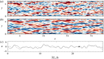
which appears in (5.1). The state-space form of (5.1) – the matrices for which are given in appendix A – allows the same optimal estimator described in § 3 to be formed and applied. Results are shown in figure 2, which follows the same template as figure 1. (The estimator performance at
 $z^{+}=101$
and at
 $z^{+}=297$
are also provided as movies.) We see that the simple eddy viscosity model leads to a significant improvement in the estimator performance.


5.4 Estimator performance in Fourier space
For convenience we will refer to the linear model (2.1) as LM1 and the linear model (5.1) as LM2 in all of the results to follow. Having looked at estimation in physical space, we now look at the two linear estimators’ performance in Fourier space at each wavenumber pair considered (
 $|k_{x}|\leqslant 8$
,
 $|k_{y}|\leqslant 64/3$
). To do this we must first introduce a measure of performance at a single wavenumber pair:
 $$\begin{eqnarray}\unicode[STIX]{x1D6FE}=\frac{\Vert \boldsymbol{e}\Vert _{2}}{\Vert \boldsymbol{z}\Vert _{2}},\end{eqnarray}$$
with the 2-norm of a time series
 $\boldsymbol{z}(t)$
defined as
 $\Vert \boldsymbol{z}\Vert _{2}=[\int \boldsymbol{z}^{\ast }(t)\boldsymbol{z}(t)\,\text{d}t]^{1/2}$
. Therefore
 $\unicode[STIX]{x1D6FE}$
is the 2-norm of the estimation error
 $\boldsymbol{e}$
normalized by the 2-norm of the velocity field
 $\boldsymbol{z}$
that is being estimated. In order to achieve better convergence, we calculate
 $\unicode[STIX]{x1D6FE}$
in each of the two halves of the channel and average over the two. The estimator is initialized with a velocity field that is zero everywhere. (This is clearly seen in all of the supplementary movies available at https://doi.org/10.1017/jfm.2018.129.) This means that there is an initial transient in the estimation error. In order to minimize the effect of this transient on
 $\unicode[STIX]{x1D6FE}$
, we therefore omit the earliest time steps when calculating
 $\unicode[STIX]{x1D6FE}$
in (5.2). Specifically, the time period used is
 $0.242<t<1.296$
(or
 $5.47<\tilde{t}U_{c}/h<29.34$
). This was chosen based on an estimate of the length of the initial transient by looking at the evolution of the energy of the estimate (in physical space) with time.
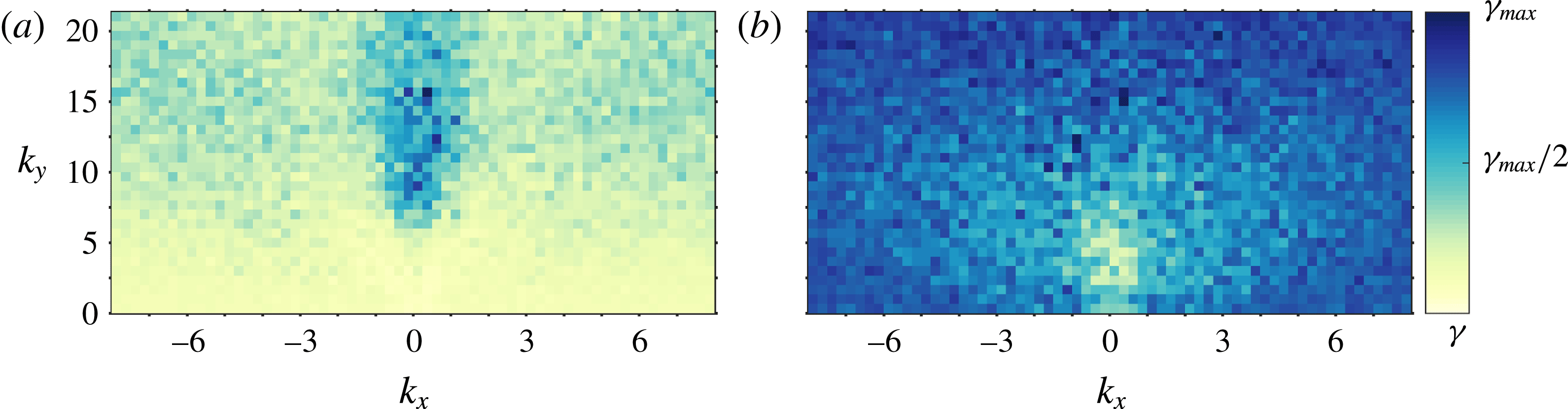
Figure 3 plots
 $\unicode[STIX]{x1D6FE}$
as a function of wavenumber pair (
 $k_{x}$
,
 $k_{y}$
) for both linear estimators. The colour scale has been chosen separately for the two estimators to accommodate the largest
 $\unicode[STIX]{x1D6FE}$
that each of them sees (which is
 $\unicode[STIX]{x1D6FE}_{max}=8.37$
for LM1 and
 $\unicode[STIX]{x1D6FE}_{max}=1.03$
for LM2). Consistent with the results in physical space in figures 1 and 2, we see that typical values of
 $\unicode[STIX]{x1D6FE}$
for LM1 are larger than those for LM2. We also see that, for LM1,
 $\unicode[STIX]{x1D6FE}$
is largest for structures with
 $|k_{x}|\approx 0$
and
 $|k_{y}|\gtrapprox 5$
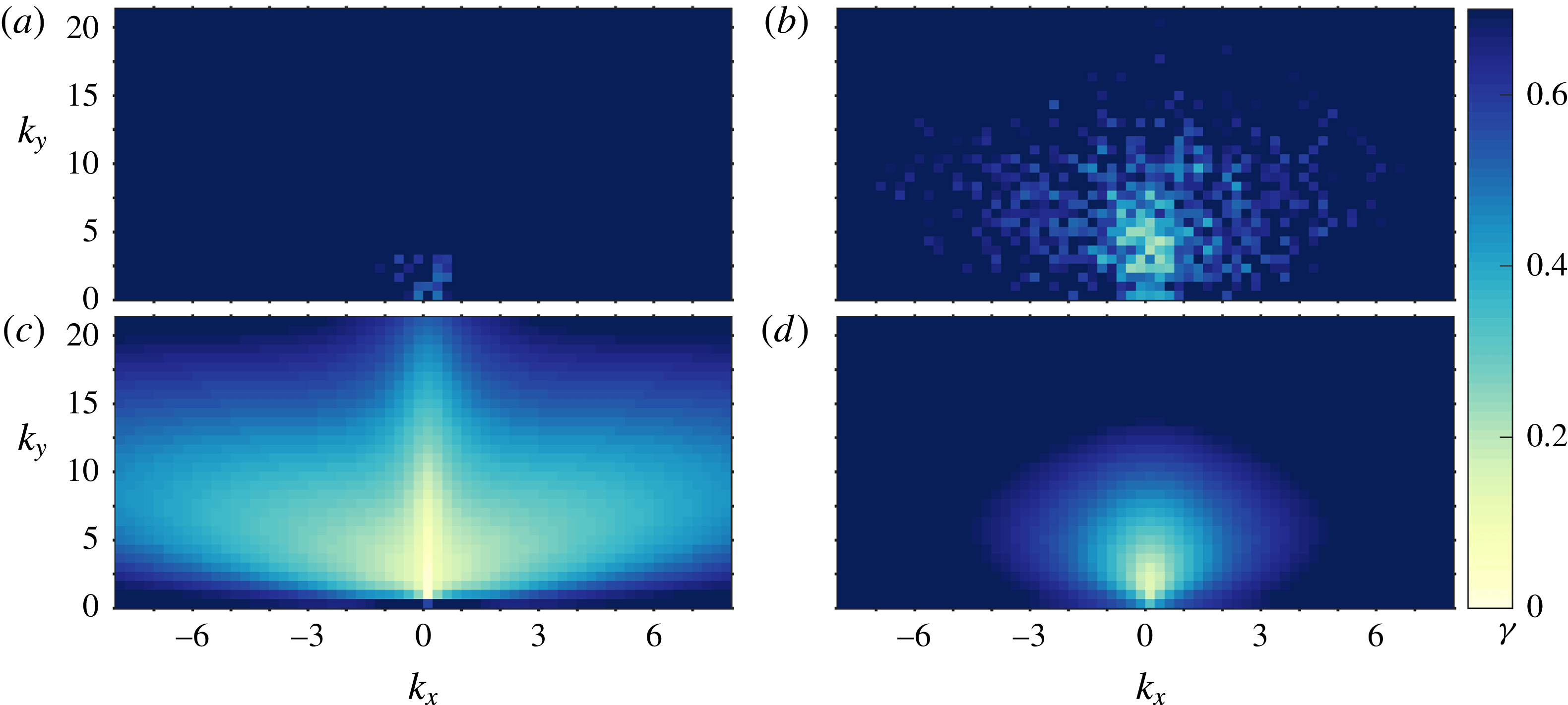
, i.e. structures that are long in the streamwise direction and thin in the spanwise direction. This is consistent with the results seen in physical space in figure 1. Figure 4(a,b) is a repeat of figure 3, this time reducing the colour scale,
 $\unicode[STIX]{x1D6FE}\in [0,0.7]$
, for both estimators. This allows us to better resolve the region over which the two estimators perform well. We see that both estimators perform best for streamwise wavenumbers
 $k_{x}\approx 0$
and spanwise wavenumbers
 $|k_{y}|\lessapprox 5$
, with LM2 performing significantly better overall. A similar analysis to that shown in figures 3 and 4 has also been performed using the correlation coefficient (between the DNS data and linear estimate) in place of the normalized error defined in (5.2). The conclusions drawn from this analysis are the same as those stated above: that LM2 performs better overall than LM1; that the best performance (for both models) is achieved for the largest structures; and that, for LM1, the performance is worst for structures that are long in the streamwise direction and relatively thin in the spanwise direction.
Normalized estimation error
 $\unicode[STIX]{x1D6FE}$
as a function of (
 $k_{x}$
,
 $k_{y}$
) for (a) LM1 (2.1); and (b) LM2 (5.1). Note that (a) and (b) use different colour scales. The value of
 $\unicode[STIX]{x1D6FE}_{max}$
(see colour bar) is (a)
 $\unicode[STIX]{x1D6FE}_{max}=8.37$
for LM1 and (b)
 $\unicode[STIX]{x1D6FE}_{max}=1.07$
for LM2.

(a,b) Normalized estimation error
 $\unicode[STIX]{x1D6FE}$
as a function of (
 $k_{x}$
,
 $k_{y}$
) for (a) LM1; and (b) LM2. (c,d) Prediction of estimation error
 $\unicode[STIX]{x1D6FE}_{pred}$
for (c) LM1; and (d) LM2. The same colour scale
 $\unicode[STIX]{x1D6FE}\in [0,0.7]$
is used for all four plots.

5.5 Estimator performance when applied to the linear model
This section is motivated by a question: Why do the linear estimators not perform better than they do? Broadly there are three possible explanations for the differences between the true velocity field and its estimate seen in figures 1 and 2.
-
(i) Linear mechanisms are not important (or not important enough).
-
(ii) Linear mechanisms are important but the linear model does not capture them.
-
(iii) Linear mechanisms are important; the linear model captures them; but there is insufficient coherence between the measurement and estimation planes.
The first two possibilities stem from the suitability of the linear model itself. The third possibility could be considered more fundamental. We mean this in the sense that if there is insufficient coherence between the measurement and estimation planes, then no estimator could perform well – the underlying physics forbids it.
If the differences seen are due to a lack of coherence, then the linear model should reproduce it. Therefore in this section, as well as designing the filter for the linear model, we also apply it to the linear model. The DNS data are thus not needed at all. We do this because we would like to know if the results seen in § 5.4 can be reproduced using nothing but a linear model. To do this we require disturbances
 $\boldsymbol{d}$
to drive the system. For the DNS results,
 $\boldsymbol{d}$
came from the terms quadratic in
 $\boldsymbol{u}$
(which were present even if unknown by the estimator). In the present case we must provide them ourselves. We do this by assuming the simplest model possible for
 $\boldsymbol{d}$
: random forcing which is white in space and white in time. We also require sensor noise but, since we expect it to be negligible for the DNS, we set
 $\boldsymbol{n}=0$
. For this choice of
 $\boldsymbol{d}$
and
 $\boldsymbol{n}$
, the 2-norm of the estimation error is given simply by
 $\Vert \boldsymbol{e}\Vert _{2}=\Vert \unicode[STIX]{x1D642}_{\boldsymbol{d}}\Vert _{2}$
, where
 $\unicode[STIX]{x1D642}_{\boldsymbol{d}}$
is the portion of
 $\unicode[STIX]{x1D642}$
in (3.3) corresponding to the transfer function from
 $\boldsymbol{d}$
to
 $\boldsymbol{e}$
. Since we want to predict the normalized error (
 $\unicode[STIX]{x1D6FE}$
), we must divide this by the 2-norm of
 $\boldsymbol{z}$
(i.e. the velocity field being estimated), which is given by
 $\Vert \boldsymbol{z}\Vert _{2}=\Vert \unicode[STIX]{x1D64B}_{z}\Vert _{2}$
. The quantity of interest is therefore
 $$\begin{eqnarray}\unicode[STIX]{x1D6FE}_{pred}=\frac{\Vert \unicode[STIX]{x1D642}_{\boldsymbol{d}}\Vert _{2}}{\Vert \unicode[STIX]{x1D64B}_{z}\Vert _{2}},\end{eqnarray}$$
which is plotted as a function of (
 $k_{x}$
,
 $k_{y}$
) for both estimators in figure 4(c,d). The same colour scale as figure 4(a,b) is used. We see that LM1 predicts good performance over a wider range of (
 $k_{x}$
,
 $k_{y}$
) pairs than it achieves with the DNS data. For LM2 there is good agreement between the performance it predicts and the performance it achieves.
5.6 Linking the estimator performance to existing results
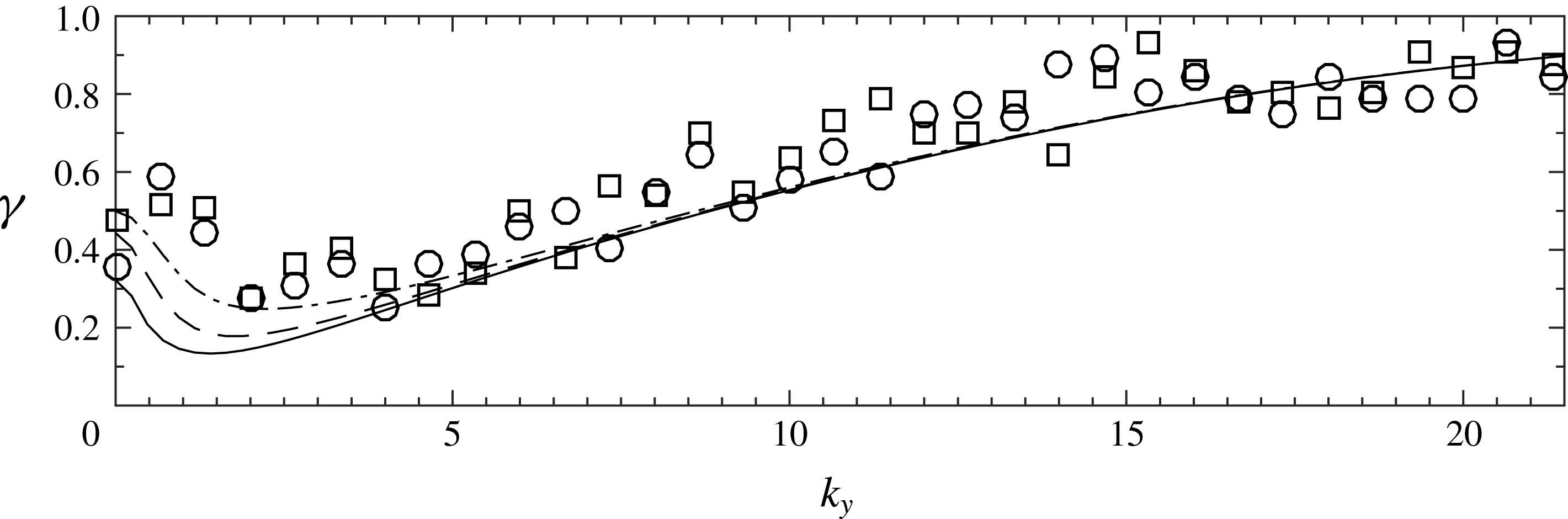
We highlight here links with previous studies that have considered a linear model with eddy viscosity. To do this we plot two quantities (for LM2 only) in figure 5. The first is the prediction of the LM2 estimation error
 $\unicode[STIX]{x1D6FE}_{pred}$
as a function of
 $k_{y}$
for
 $k_{x}=0$
,
 $k_{x}=\pm 0.25$
and
 $k_{x}=\pm 0.5$
. The second is the true estimation error
 $\unicode[STIX]{x1D6FE}$
achieved in DNS where, in order to reduce scatter in the plot, we average
 $\unicode[STIX]{x1D6FE}$
across all
 $|k_{x}|\leqslant 0.5$
for each value of
 $k_{y}$
. The average is therefore performed across five realizations:
 $k_{x}=0$
,
 $k_{x}=\pm 0.25$
and
 $k_{x}=\pm 0.5$
. We also plot the results for each half of the channel separately to give some idea of the scatter in the results. We see that the spanwise wavenumber at which the predicted estimation error
 $\unicode[STIX]{x1D6FE}_{pred}$
attains its minimum is in the range
 $k_{y}=1.4{-}2.1$
(specifically
 $k_{y}=1.4$
for
 $k_{x}=0$
;
 $k_{y}=1.9$
for
 $k_{x}=\pm 0.25$
; and
 $k_{y}=2.1$
for
 $k_{x}=\pm 0.5$
), which corresponds to
 $\unicode[STIX]{x1D706}_{y}=3.0{-}4.5$
. This is in reasonable agreement with the results achieved in DNS (notwithstanding the scatter in the data) and provides an important link to existing results in the literature. Pujals et al. (Reference Pujals, García-Villalba, Cossu and Depardon2009) look at optimal transient growth for a linear model with eddy viscosity (LM2) over a range of Reynolds numbers,
 $500\leqslant Re_{\unicode[STIX]{x1D70F}}\leqslant 20\,000$
. They find that, for streamwise-constant structures (
 $k_{x}=0$
), the maximum transient growth is attained for a spanwise wavenumber of
 $k_{y}\approx \unicode[STIX]{x03C0}/2$
(
 $\unicode[STIX]{x1D706}_{y}\approx 4.0$
) for all Reynolds numbers considered. Hwang & Cossu (Reference Hwang and Cossu2010b
), meanwhile, find the energy amplification achieved by optimal harmonic and stochastic forcing for the same linear model (LM2) and over the same range of Reynolds numbers (
 $500\leqslant Re_{\unicode[STIX]{x1D70F}}\leqslant 20\,000$
). For
 $k_{x}=0$
they find that the most amplified structures have a spanwise wavenumber of
 $k_{y}\approx 1.8$
(
 $\unicode[STIX]{x1D706}_{y}\approx 3.5$
). To summarize, the structures that are best estimated by the linear estimator coincidence well with the structures that (i) have the greatest potential for transient growth (Pujals et al.
Reference Pujals, García-Villalba, Cossu and Depardon2009); and (ii) are most amplified in the stochastically forced and harmonically forced settings (Hwang & Cossu Reference Hwang and Cossu2010b
).
Prediction of the LM2 estimator performance
 $\unicode[STIX]{x1D6FE}_{pred}$
as a function of
 $k_{y}$
for
 $k_{x}=0$
(——),
 $k_{x}=\pm 0.25$
(– –) and
 $k_{x}=\pm 0.5$
(–
 $\cdot$
–); and true estimator performance
 $\unicode[STIX]{x1D6FE}$
averaged over all
 $k_{x}\leqslant |0.5|$
for the two halves of the channel (○, ▫).

5.7 Estimator performance across wall heights
We have looked at the estimator performance at
 $z^{+}=101$
in §§ 5.2 and 5.3; and at
 $z^{+}=101$
and
 $z^{+}=297$
in § 5.4. (Recall that measurements are taken at
 $z^{+}=197$
.) We now look at the estimator performance across a range of wall-normal heights, keeping the measurement location at
 $z^{+}=197$
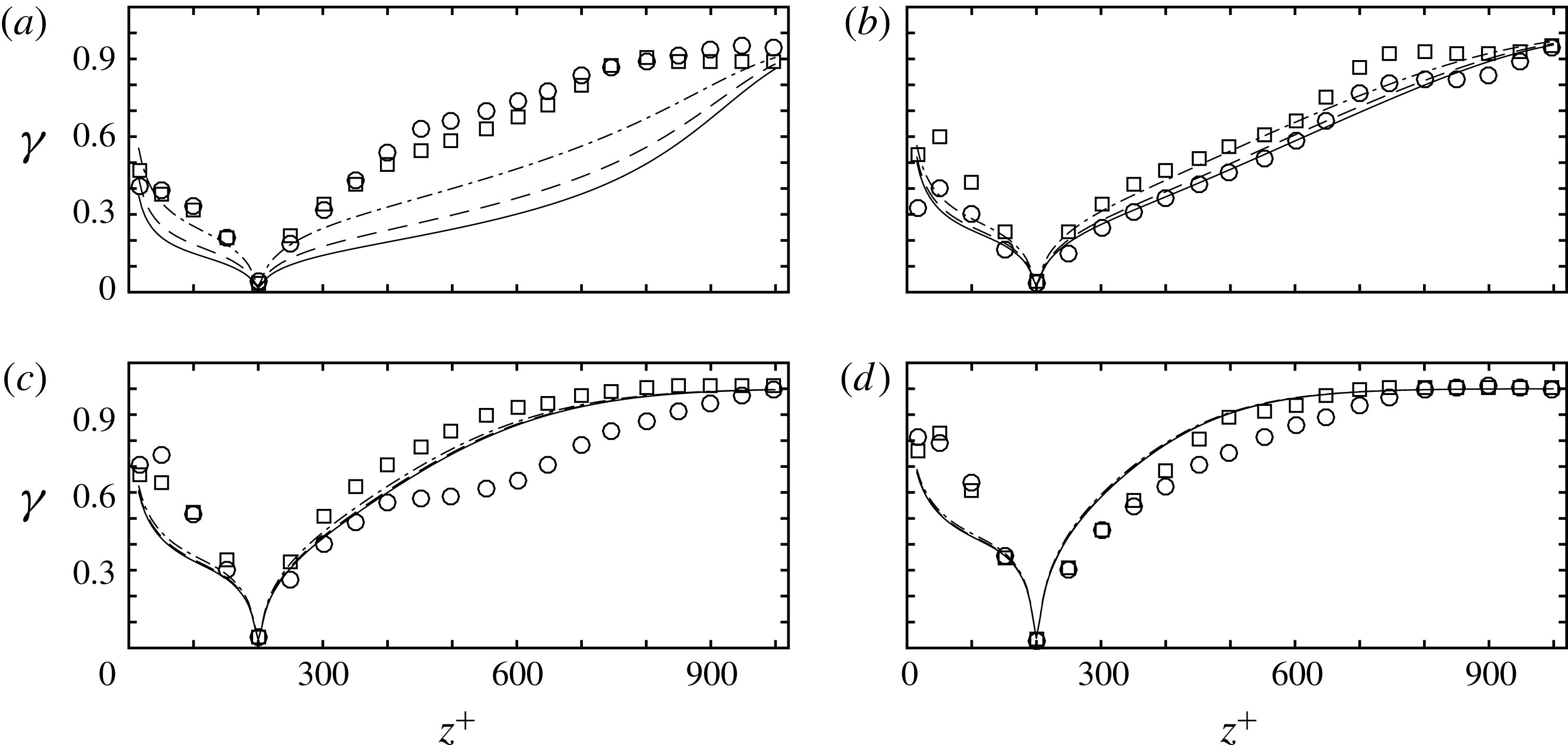
throughout. To do this we follow the template of figure 5 and plot two quantities, but this time as a function of wall height
 $z^{+}$
. The first is the prediction of the LM2 estimation error,
 $\unicode[STIX]{x1D6FE}_{pred}$
, as a function of wall height for
 $k_{x}=0$
,
 $k_{x}=\pm 0.25$
and
 $k_{x}=\pm 0.5$
. The second is the true estimation error
 $\unicode[STIX]{x1D6FE}$
achieved in DNS. Like figure 5 we average
 $\unicode[STIX]{x1D6FE}$
across all
 $|k_{x}|\leqslant 0.5$
for each wall height to reduce scatter in the results; and like figure 5 we plot the results for each half of the channel separately. These quantities are plotted in figure 6 for four values of the spanwise wavenumber,
 $k_{y}=2$
, 4, 6 and 8. As one would expect, the estimator performs best for wall heights near
 $z^{+}=197$
, with the estimation error
 $\unicode[STIX]{x1D6FE}$
increasing monotonically away from this location. We see good agreement between the predicted estimation error and that achieved in DNS, particularly for
 $k_{y}=4$
, 6 and 8 (with scatter in the DNS results as before). For
 $k_{y}=2$
and wall heights towards the centre of the channel we see that the estimator does not perform quite as well as predicted. Nevertheless the true estimator performance for
 $k_{y}=2$
is competitive with that for
 $k_{y}=4$
, 6 and 8. The results of figure 6 provide useful information on the estimator performance with wall height; and also provide further evidence that the linear model (5.1) is able to reproduce important features of the estimation problem.
Prediction of the LM2 estimator performance
 $\unicode[STIX]{x1D6FE}_{pred}$
as a function of wall-normal location
 $z^{+}$
for
 $k_{x}=0$
(—),
 $k_{x}=\pm 0.25$
(– –) and
 $k_{x}=\pm 0.5$
(–
 $\cdot$
–); and true estimator performance
 $\unicode[STIX]{x1D6FE}$
averaged over all
 $k_{x}\leqslant |0.5|$
for the two halves of the channel (○, ▫). This is plotted for (a)
 $k_{y}=2$
; (b)
 $k_{y}=4$
; (c)
 $k_{y}=6$
; and (d)
 $k_{y}=8$
.

5.8 Discussion
It is important to stress that estimation has been performed only for the largest scales. Specifically, and as stated in § 4, we have considered only wavenumbers satisfying
 $|k_{x}|\leqslant 8$
and
 $|k_{y}|\leqslant 64/3$
(
 $\unicode[STIX]{x1D706}_{x}\geqslant 0.785$
and
 $\unicode[STIX]{x1D706}_{y}\geqslant 0.295$
). The results of figure 4(b,d) show that this choice makes sense since, for the wall-normal heights considered, these are the only scales for which we expect the estimator to be successful. For these largest scales the performance of the linear estimator is improved by including an eddy viscosity in the linear model. This suggests that, for successful estimation, it is important to model the influence of the small-scale turbulence on the large-scale coherent motions of interest. Put another way, it is important to impose structure on the feedback between the velocity field and the Reynolds stresses to which it gives rise – and even a very simple model to impose this structure improves estimator performance significantly.
For the smallest scales, in contrast, one would anticipate that the kinematic viscosity alone is the most appropriate viscosity model, since here any eddy viscosity would be accounting for the very scales one wishes to resolve. The question then naturally arises as to what one should do for the intermediate scales. One option would be to use a wavenumber-dependent eddy viscosity. In the present linear modelling context the recent work of Zare et al. (Reference Zare, Jovanovic and Georgiou2017) is particularly relevant, which provides a data-driven refinement of a Navier–Stokes-based linear model to account for second-order statistics. It would be interesting to use this approach in the linear estimation problem considered here.
We finish this section by considering the performance (and predicted performance) of the LM2-based estimator for large values of
 $|k_{x}|$
and
 $|k_{y}|$
(i.e. small structures). We observe that the normalized estimation error,
 $\unicode[STIX]{x1D6FE}$
, is largest for the largest values of
 $|k_{x}|$
and for the largest values of
 $|k_{y}|$
, i.e. structures that are small in at least one of the two homogeneous directions. This is clearly seen in figure 4, where
 $\unicode[STIX]{x1D6FE}$
is largest when
 $|k_{x}|$
is large or
 $|k_{y}|$
is large; in figure 5, where
 $\unicode[STIX]{x1D6FE}$
increases for increasing
 $k_{y}$
; and in figure 6 where, for individual (
 $k_{x}$
,
 $k_{y}$
) pairs,
 $\unicode[STIX]{x1D6FE}$
increases as the estimation plane is placed further away from the measurement plane (i.e. as the structures become smaller relative to this separation distance). One can understand this physically in the following way. When the size of the structure to be estimated becomes too small (relative to the distance between the estimation and measurement planes), the estimation task becomes very difficult. This is not only because the linear operator corresponding to (5.1) shows smaller amplification for these smaller structures (equivalently, nonlinear mechanisms are more important), but also because any such structure is presumably more localized in the wall-normal direction.
6 Conclusions
Using a linear, Navier–Stokes-based model of channel flow at
 $Re_{\unicode[STIX]{x1D70F}}=1000$
it is possible to estimate the largest scales with reasonable accuracy when a simple eddy viscosity model is included. For the flow under consideration, then, linear mechanisms are sufficiently important to the large scales that a linear model is able to model and estimate them with reasonable accuracy. Importantly, the linear model with eddy viscosity not only improves the performance of the estimator, but is also able to predict the range of wavenumber pairs (figure 4) and the range of wall heights (figure 6) over which the estimator should perform well. This is compelling evidence that the model captures the underlying physics of the large scales, as discussed in § 5.5. The structures that are best estimated coincide well with the structures that show the greatest potential for amplification in both the transient growth and externally forced settings. The results suggest that there is merit in further efforts towards estimation and control of large-scale structures in wall-bounded turbulent flows.
Acknowledgements
The authors are grateful for the financial support of the Australian Research Council.
Supplementary movies
Supplementary movies are available at https://doi.org/10.1017/jfm.2018.129.
Appendix A. State-space form of the linear models
The state-space representation (2.3) of the linear model (2.1) is
 $$\begin{eqnarray}\displaystyle & \displaystyle \frac{\text{d}}{\text{d}t}\left[\begin{array}{@{}c@{}}\hat{\boldsymbol{w}}\\ \hat{\boldsymbol{\unicode[STIX]{x1D702}}}\end{array}\right]=\left[\begin{array}{@{}cc@{}}\unicode[STIX]{x1D6E5}^{-1}{\mathcal{L}}_{OS} & 0\\ -\text{i}k_{y}U^{\prime } & {\mathcal{L}}_{SQ}\end{array}\right]\left[\begin{array}{@{}c@{}}\hat{\boldsymbol{w}}\\ \hat{\boldsymbol{\unicode[STIX]{x1D702}}}\end{array}\right]+\left[\begin{array}{@{}ccc@{}}-\text{i}k_{x}\unicode[STIX]{x1D6E5}^{-1}{\mathcal{D}} & -\text{i}k_{y}\unicode[STIX]{x1D6E5}^{-1}{\mathcal{D}} & -k^{2}\unicode[STIX]{x1D6E5}^{-1}\\ \text{i}k_{y} & -\text{i}k_{x} & 0\end{array}\right]\left[\begin{array}{@{}c@{}}\hat{\boldsymbol{d}}_{x}\\ \hat{\boldsymbol{d}}_{y}\\ \hat{\boldsymbol{d}}_{z}\end{array}\right],\qquad & \displaystyle\end{eqnarray}$$
 $$\begin{eqnarray}\displaystyle & \displaystyle \left[\begin{array}{@{}c@{}}\hat{\boldsymbol{u}}\\ \hat{\boldsymbol{v}}\\ \hat{\boldsymbol{w}}\end{array}\right]=\frac{1}{k^{2}}\left[\begin{array}{@{}cc@{}}\text{i}k_{x}{\mathcal{D}} & -\text{i}k_{y}\\ \text{i}k_{y}{\mathcal{D}} & \text{i}k_{x}\\ k^{2} & 0\end{array}\right]\left[\begin{array}{@{}c@{}}\hat{\boldsymbol{w}}\\ \hat{\boldsymbol{\unicode[STIX]{x1D702}}}\end{array}\right], & \displaystyle\end{eqnarray}$$
 $\hat{\boldsymbol{w}}(t)=\unicode[STIX]{x2202}_{z}\hat{\boldsymbol{w}}(t)=\hat{\boldsymbol{\unicode[STIX]{x1D702}}}(t)=0$
at the two walls. Here
 ${\mathcal{D}}$
and
 $^{\prime }$
represent differentiation in the wall-normal direction;
 $k^{2}=k_{x}^{2}+k_{y}^{2}$
;
 $\unicode[STIX]{x1D6E5}={\mathcal{D}}^{2}-k^{2}$
is the Laplacian; and
 ${\mathcal{L}}_{OS}$
and
 ${\mathcal{L}}_{SQ}$
are the Orr–Sommerfeld and Squire operators:
 $$\begin{eqnarray}\displaystyle & \displaystyle {\mathcal{L}}_{OS}=-\text{i}k_{x}U\unicode[STIX]{x1D6E5}+\text{i}k_{x}U^{\prime \prime }+Re_{\unicode[STIX]{x1D70F}}^{-1}\unicode[STIX]{x1D6E5}^{2}, & \displaystyle\end{eqnarray}$$
 $$\begin{eqnarray}\displaystyle & \displaystyle {\mathcal{L}}_{SQ}=-\text{i}k_{x}U+Re_{\unicode[STIX]{x1D70F}}^{-1}\unicode[STIX]{x1D6E5}. & \displaystyle\end{eqnarray}$$
 $$\begin{eqnarray}\displaystyle & \displaystyle {\mathcal{L}}_{OS}=-\text{i}k_{x}U\unicode[STIX]{x1D6E5}+\text{i}k_{x}U^{\prime \prime }+\unicode[STIX]{x1D708}_{T}\unicode[STIX]{x1D6E5}^{2}+2\unicode[STIX]{x1D708}_{T}^{\prime }{\mathcal{D}}\unicode[STIX]{x1D6E5}+\unicode[STIX]{x1D708}_{T}^{\prime \prime }({\mathcal{D}}^{2}+k^{2}), & \displaystyle\end{eqnarray}$$
 $$\begin{eqnarray}\displaystyle & \displaystyle {\mathcal{L}}_{SQ}=-\text{i}k_{x}U+\unicode[STIX]{x1D708}_{T}\unicode[STIX]{x1D6E5}+\unicode[STIX]{x1D708}_{T}^{\prime }{\mathcal{D}}. & \displaystyle\end{eqnarray}$$
A.1 Output matrices
 $\unicode[STIX]{x1D63E}_{y}$
and
$\unicode[STIX]{x1D63E}_{z}$


Since Chebyshev discretization is used in the wall-normal direction (see § 2.1), (A 1b
) gives the three velocity components at the Chebyshev collocation points. In general these do not coincide with the wall-normal locations of interest. Therefore a modification of (A 1b
) must be made so that the state-space matrices
 $\unicode[STIX]{x1D63E}_{y}$
(for measurement locations) and
 $\unicode[STIX]{x1D63E}_{z}$
(for estimation locations) introduced in (3.1) can be formed for any wall height of interest. This is achieved by implementing barycentric Lagrange interpolation (Berrut & Trefethen Reference Berrut and Trefethen2004) as a matrix operation. This matrix premultiplies the matrix in (A 1b
) to give the three velocity components at the wall heights of interest. In this way the matrices
 $\unicode[STIX]{x1D63E}_{y}$
and
 $\unicode[STIX]{x1D63E}_{z}$
in (3.1) can be formed for any measurement locations and for any estimation locations of interest.
Appendix B. Estimator design
Here we give further details on how the filter
 $\unicode[STIX]{x1D641}$
in § 3 is formed. We first take the block diagram in (3.3) and put it in the standard form shown below (Doyle et al.
Reference Doyle, Glover, Khargonekar and Francis1989):

with
 $\unicode[STIX]{x1D64B}_{\boldsymbol{z}}$
and
 $\unicode[STIX]{x1D64B}_{\boldsymbol{y}}$
as defined in (3.2). (Note that
 $\unicode[STIX]{x1D642}(s)$
in (B 1) is the same as
 $\unicode[STIX]{x1D642}(s)$
in (3.3), although
 $\unicode[STIX]{x1D642}(s)$
in (3.3) was not weighted to simplify the discussion there.) Weighting matrices
 $\unicode[STIX]{x1D652}_{\boldsymbol{d}}$
and
 $\unicode[STIX]{x1D652}_{\boldsymbol{n}}$
are included in
 $\tilde{\unicode[STIX]{x1D64B}}$
. These can be used to prioritize certain input directions and frequency ranges (for both disturbances and noise) that one wishes to guard against; and to rescale disturbances
 $\boldsymbol{d}$
and noise
 $\boldsymbol{n}$
to reflect their relative sizes. We set
 $\unicode[STIX]{x1D652}_{\boldsymbol{d}}=\unicode[STIX]{x1D644}$
and
 $\unicode[STIX]{x1D652}_{\boldsymbol{n}}=\unicode[STIX]{x1D6FC}_{\boldsymbol{n}}\unicode[STIX]{x1D644}$
. (Recall from § 3 that the 2-norm (3.4) to be minimized is defined such that it corresponds to a grid-independent energy-norm.) This amounts to a design choice to guard against all input directions and all frequencies equally for both disturbances and noise. The parameter
 $\unicode[STIX]{x1D6FC}_{\boldsymbol{n}}$
allows one to set the expected size of the sensor noise relative to disturbances. We expect sensor noise in the direct numerical simulations to be negligible, but we must set
 $\unicode[STIX]{x1D6FC}_{\boldsymbol{n}}>0$
so that the estimator design procedure is well-posed. We therefore set
 $\unicode[STIX]{x1D6FC}_{\boldsymbol{n}}$
such that the variance of the sensor noise is 1 % of the variance of the measurements. With the overall transfer function
 $\tilde{\unicode[STIX]{x1D64B}}$
formed, we are now in a position to design the filter
 $\unicode[STIX]{x1D641}(s)$
. Recall from § 3 that the design task is: given
 $\unicode[STIX]{x1D64B}$
(and therefore
 $\tilde{\unicode[STIX]{x1D64B}}$
in (B 1)), design
 $\unicode[STIX]{x1D641}$
such that
 $\unicode[STIX]{x1D642}$
is small. More specifically,
 $\unicode[STIX]{x1D641}$
is designed such that the 2-norm of
 $\unicode[STIX]{x1D642}$
in (B 1) is minimized. This is achieved in practice by using
 $\tilde{\unicode[STIX]{x1D64B}}$
in state-space form to solve a pair of algebraic Riccati equations. For more details on the solution procedure for
 $\unicode[STIX]{x1D641}(s)$
see Doyle et al. (Reference Doyle, Glover, Khargonekar and Francis1989) or Zhou & Doyle (Reference Zhou and Doyle1998, chap. 13).