I. INTRODUCTION
The nanoindentation technique is widely used to measure the hardness H and the reduced elastic modulus E ′* of materials at the nanometer scale. The first hardness tests were realized by Brinell, who used a hard steel sphere to indent samples (see TaborReference Tabor1). Other hardness tests were developed later, such as the Vickers test or the Knoop test, which differ in the indenter geometry.Reference Tabor2 To measure hardness, the load and the projected contact area have to be known. For these tests, the load is imposed, and the contact area is measured after the test with an optical microscope. At a smaller scale, optical measurement of the contact area is not precise enough, so instrumented indentation testing has been developed. With instrumented nanoindentation testing, the load P and the displacement h m are measured continuously during the test. With this technique, which is based on load and displacement measurement, Bulychev et al.Reference Bulychev, Alekhin, Shorshorov, Ternovskii and Shnyrev3 showed that the reduced elastic modulus of the material can be obtained from the unloading curve. A great number of authors have contributed to the understanding of the loading–unloading curves with new methods of analysis.Reference Loubet, Bauer, Tonck, Bec and Gauthier-Manuel4–Reference Pethica, Hutchings and Oliver10
The past 20 years or so have seen the development of a dynamic technique called Continuous Stiffness Measurement (CSM).Reference Oliver and Pharr6 The principle is to superimpose a small oscillation amplitude on the displacement (or load) signal and to measure the load (or displacement) response. The harmonic contact stiffness and the harmonic contact damping of the tested material can be computed from the analysis of the dynamic response of the system. Viscoelastic properties are thus obtained with the CSM method, which is useful for polymeric materials characterization.Reference Asif, Wahl and Colton11 In addition, with the CSM technique, mechanical properties can be measured as a function of the indentation depth, which is helpful for the characterization of coatings or graded materials.
To compute the static and dynamic properties cited above, the projected contact area value is necessary. With the nanoindentation technique, the tip displacement is measured, not the contact depth or the projected contact area. Many methods to estimate this area have been proposed, but a lot of uncertainties related to the displacement measurement influence the data, which is problematic for contact area measurement, particularly at small penetration depths (see Sec. II). This paper presents a new technique based on the detection of the amplitude of the second harmonic. This technique was already suggested in a previous paper, in which the equations were written as a function of the derivative of the contact radius versus indentation depth.Reference Guillonneau, Kermouche, Bec and Loubet12 Mechanical properties were more precise at smaller penetration depths, but the proposed equations were applicable only for materials with a constant H/E c′* ratio (E c′* is the reduced contact modulus between the tip and the sample). This paper presents an improved technique that does not use the indentation depth and thus is applicable to any materials with constant reduced elastic modulus.
In this paper, we begin by the discussion of the projected contact area calculation and the uncertainties related to the displacement measurement. It is followed by the unloading curve study to show how it is possible to compute the elastic modulus, the hardness, and the indentation depth without any use of the indentation depth. The fourth part explains the link between the elastic modulus and the amplitude of the second harmonic. The fifth part presents the experimental tests, and the sixth part discusses the results.
II. DETERMINATION OF THE PROJECTED CONTACT AREA
A. Mechanical properties measured with the CSM method
With instrumented nanoindentation testing, the hardness H, the reduced elastic contact modulus E c′*, and the loss contact modulus E c″* of tested materials are computed as a function of the indentation depth. The hardness is defined as the load divided by the projected contact area between the indenter and the sampleReference Tabor1, Reference Oliver and Pharr6, Reference Asif, Wahl and Colton11, Reference Guillonneau, Kermouche, Bec and Loubet12:
 $$![CDATA[$$H = \hskip1pt{P \over {A_{\rm{c}} }},$$
where P is the applied load and A c is the projected contact area. The reduced elastic contact modulus can be computed using the Sneddon relationReference Sneddon13:
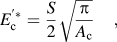 $$![CDATA[$$E_{\rm{c}}^{\prime*} =\hskip1pt {S \over 2}\sqrt {{{\rm{\pi }} \over {A_{\rm{c}} }}} ,$$
where S is the harmonic contact stiffness measured continuously with the CSM technique. This equation is valid for any axisymmetric indenter. The loss modulus is defined by the following equationReference Lucas, Oliver, Pharr, Loubet, Gerberich, Gao, Sundgren and Baker14, Reference Fischer-Cripps15:
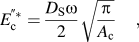 $$![CDATA[$$E_{\rm{c}}^{\Prime*} = {{D_{\rm{S}} {\rm{\omega }}} \over 2}\sqrt {{{\rm{\pi }} \over {A_{\rm{c}} }}} ,$$
where D s is the harmonic contact damping and ω is the angular frequency. Equations (2) and (3) can be multiplied by a constant coefficient to take into account the nonaxisymmetry of the indenter.Reference Oliver and Pharr8, Reference Fischer-Cripps15, Reference King16 With the static method, the hardness and the reduced elastic contact modulus are obtained at maximum load. With the CSM technique, the mechanical properties described by Eqs. (1)–(3) are measured as a function of the indentation depth h. All equations depend on the projected contact area A c. With a perfect conical indenter, the projected contact area A c can be calculated from the contact depth h c using a geometrical relation:
 $$![CDATA[$$A_{\rm{c}} = {\rm{\pi }}(\tan ({\rm{\theta }})h_{\rm{c}} )^2 ,$$
where θ is the equivalent angle of the conical indenter (for a Berkovich tip, θ = 70.32°). In instrumented nanoindentation, the contact depth h c is computed from the indentation depth value h. The calculation of the actual contact depth is very difficult because the relation between the contact depth and the indentation depth is influenced by measurement uncertainties (thermal drift, tip defect, etc.) and by material pileup or sink-in around the indent during the test. A lot of methods can be used to precisely determine this relation. The Oliver and Pharr modelReference Oliver and Pharr6 is the mainly used method. The contact depth is defined by the following equation:
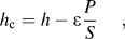 $$![CDATA[$$h_{\rm{c}} = h - {\rm{\varepsilon }}{P \over S},$$
where h is the indentation depth and ε is a constant depending on the indenter geometry. Then, Oliver and Pharr propose computing the projected contact area with an area function, which takes into account the nonperfect geometry of the indenter.Reference Oliver and Pharr6 Loubet et al.Reference Bec, Tonck, Georges, Georges and Loubet17, Reference Hochstetter, Jimenez and Loubet18 propose another method. The relation between the contact depth and the indentation depth is given by the following equation:
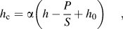 $$![CDATA[$$h_{\rm{c}} = {\rm{\alpha }}\left( {h - {P \over S} + h_0 } \right),$$
where h 0 is an equivalent height of the tip defect. Piling-up and sinking-in phenomena are taken into account by the coefficient α, the value of which is 1.2 for a Berkovich indenter.Reference Bec, Tonck, Georges, Georges and Loubet17 The Loubet model can be used for a large range of materials. We note that the ratio P/S can be written as a function of hardness, reduced elastic modulus, and contact depth by combining Eqs. (1), (2), and (4):
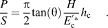 $$![CDATA[$${P \over S} = {{\rm{\pi }} \over 2}\tan ({\rm{\theta }}){H \over {E_{\rm{c}}^{\prime*} }}h_{\rm{c}} .$$
This relation will be used in Sec. III.
B. Displacement uncertainties
To determine the indentation depth h, the precise identification of the contact point h in is necessary. The indentation depth is related to the measured tip displacement h m by the following equation:
 $$![CDATA[$$h = h_{\rm{m}} - h_{{\rm{in}}} .$$
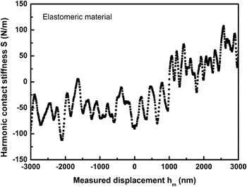
Plotting the harmonic contact stiffness S versus the measured displacement h m is one way of identifying the contact point.Reference Oliver and Pharr8 When an abrupt increase of the harmonic contact stiffness is detected, the indenter is considered to be in contact with the sample. For very soft materials, however, contact detection is difficult. In Fig. 1, the harmonic contact stiffness of an elastomeric material is plotted versus the measured displacement h m. Because of the low stiffness of the material, the contact point is difficult to detect; the contact detection error can reach 100 nm or more, inducing an error on the calculation of the projected contact area, and consequently on the mechanical properties, especially at small indentation depths.
Harmonic contact stiffness versus measured displacement h m for an elastomeric material. The precise contact point is difficult to identify, so an error of 100 nm or more is possible.

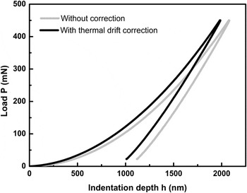
A second uncertainty comes from the thermal drift caused by temperature variation during the test (Fig. 2), which induces contraction or dilatation of the sample, the indenter, and other components such as the frame. The most commonly used method to cope with this problem is to place the tip on the surface, then to hold the load at a low constant value of a few micronewtons during a period of 100 s, while the displacement is monitored to identify the displacement rate produced by thermal expansion in the system.Reference Oliver and Pharr6 Other techniques can be used to account for the thermal drift.Reference Fischer-Cripps15 All the cited methods suppose that the thermal drift is constant during the test.
Loading–unloading curve with and without thermal drift correction. Usual proposed corrections require assuming a constant thermal drift during the test.

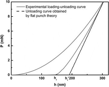
A third uncertainty is the tip defect. Indeed, the indenter is not perfectly sharp, so geometrical relation is not adapted to compute the contact area. To estimate the equivalent height of the tip defect, Loubet et al.Reference Bec, Tonck, Georges, Georges and Loubet17 suggest plotting the dynamic contact stiffness versus penetration depth h r′ [the penetration depth is defined in Fig. 3 and in Eq. (11) in Ref. Reference Guillonneau, Kermouche, Bec and Loubet12] using a flat homogeneous material like fused silica. Indeed, for a perfectly sharp indenter, the dynamic contact stiffness is expected to vary proportionally to the penetration depth, which is not the case for rounded tips. Loubet et al. propose extrapolating to zero the linear part of the stiffness curve versus penetration depth to obtain the depth h 0 corresponding to the equivalent height of the tip defect. This value h 0 is then added to the calculated penetration depth to account for the tip defect. Nevertheless, at penetration depths lower than 100 nm, the error in h 0 calculation has great influence on the calculation of the projected contact area.Reference Guillonneau, Kermouche, Bec and Loubet12 Thus, h 0 needs to be precisely computed to obtain reliable hardness values. However, for penetration depths lower than 20–30 nm, because of the nonperfect geometry of the indenter, the tip cannot be considered as a Berkovich indenter, so Eq. (4) cannot be used to calculate the projected contact area.
Loading–unloading curve of fused silica with a Berkovich tip. The dashed line is the theoretical unloading curve obtained with a flat punch; h r is the remanent depth and h r′ is the penetration depth.

In a recent paper,Reference Guillonneau, Kermouche, Bec and Loubet12 we proposed a new method that eliminates all these uncertainties. This method was based on the measurement of the displacement second harmonic amplitude but was only valid for homogeneous materials. In the present paper, we extend this method to nonhomogeneous materials by computing the mechanical properties only from dynamic measurements (i.e., CSM) and not from static measurements (i.e., indentation depth).
III. STUDY OF THE UNLOADING CURVE
Figure 3 shows a typical loading–unloading curve obtained on a fused silica sample. With the unloading part, it is possible to calculate the contact stiffness S, expressed as a function of the reduced elastic contact modulus E c′* with the following equationReference Sneddon13, Reference Fischer-Cripps15:
 $$![CDATA[$$S = 2E_{\rm{c}}^{\prime*} a,$$
where a is the equivalent tip contact radius. This expression is valid for an elastic contact for all axisymmetric indenters.Reference Pharr, Oliver and Brotzen19 If the contact radius is substituted by the contact depth h c, for a pyramid-shaped indenter, the following equation is obtained:
 $$![CDATA[$$S = 2\tan ({\rm{\theta }})E_{\rm{c}}^{\prime*} h_{\rm{c}} .$$
For indentation test with a flat punch, the stiffness is simply the slope of the unloading curve (dashed line in Fig. 3). As shown in Fig. 3, the unloading curve for a pyramid-shaped indenter is not linear, so a second derivative is computable. After derivation of Eq. (10) with respect to the indentation depth h, and assuming that the reduced elastic contact modulus is constant during the unloading, the following equation is obtained:
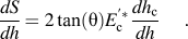 $$![CDATA[$${{dS} \over {dh}} = 2\tan ({\rm{\theta }})E_{\rm{c}}^{\prime*} {{dh_{\rm{c}} } \over {dh}}.$$
This expression depends on the indenter geometry, on the reduced elastic contact modulus, and on the derivative of the contact depth h c with respect to the indentation depth h. The last term is of primary importance, as it takes into account the pileup or sink-in of the material. The Loubet contact depth model in Eq. (7) yields to:
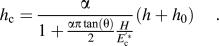 $$![CDATA[$$h_{\rm{c}} = {{\rm{\alpha }} \over {1 + {{{\rm{\alpha \pi }}\tan ({\rm{\theta }})} \over 2}{H \over {E_{\rm{c}}^{\prime*} }}}}(h + h_0 ).$$
After derivation of Eq. (12) with respect to the indentation depth h, the following equation is obtained:
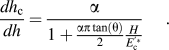 $$![CDATA[$${{dh_{\rm{c}} } \over {dh}} = {{\rm{\alpha }} \over {1 + {{{\rm{\alpha \pi }}\tan ({\rm{\theta }})} \over 2}{H \over {E_{\rm{c}}^{\prime*} }}}}.$$
The hardness H can also be substituted in Eq. (13) by the following expression:
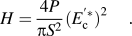 $$![CDATA[$$H = {{4P} \over {{\rm{\pi }}S^2 }}(E_{\rm{c}}^{\prime*} )^2 .$$
The reduced elastic contact modulus can be then computed from Eqs. (11), (13), and (14):
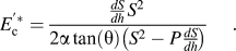 $$![CDATA[$$E_{\rm{c}}^{\prime*} = {{{{dS} \over {dh}}S^2 } \over {2{\rm{\alpha }}\tan ({\rm{\theta }})\left( {S^2 - P{{dS} \over {dh}}} \right)}}.$$
The hardness is computed with Eq. (14) and the reduced elastic modulus E ′* of the material is computed with the following equation:
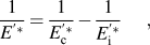 $$![CDATA[$${1 \over {E^{\prime*} }} = {1 \over {E_{\rm{c}}^{\prime*} }} - {1 \over {E_{\rm{i}}^{\prime*} }},$$
where E i′* is the reduced elastic modulus of the indenter. The displacement measurement is no longer needed, which is of primary interest regarding the uncertainties mentioned in the previous paragraph. The expression of the derivative of the contact depth with respect to the indentation depth has been computed with the Loubet model, but the same calculation can be done with the Oliver and Pharr model.
We note that the indentation depth h can be directly computed from the ratio of the harmonic contact stiffness [Eq. (10)] over the derivative of the contact stiffness versus indentation depth [Eq. (11)], by noticing that:
 $$![CDATA[$${S \mathord{\left/ {\vphantom {S {{{dS} \over {dh}}}}} \right. \kern-\nulldelimiterspace} {{{dS} \over {dh}}}} = {{h_{\rm{c}} } \mathord{\left/ {\vphantom {{h_{\rm{c}} } {{{dh_{\rm{c}} } \over {dh}} = h + h_0 .}}} \right. \kern-\nulldelimiterspace} {{{dh_{\rm{c}} } \over {dh}} = h + h_0 .}}$$
To obtain the reduced elastic modulus, the hardness, and the indentation depth without any displacement measurement, it is necessary to determine the derivative of the contact stiffness with respect to the indentation depth. The following section presents the method that we use to make such determination.
IV. SECOND DERIVATIVE AND SECOND HARMONIC (CSM METHOD)
In a previous paper, with the expression of the Fourier series and the Taylor development at the second order, it was shown how to link the second derivative of load with respect to the indentation depth with the second harmonic of loadReference Guillonneau, Kermouche, Bec and Loubet12:
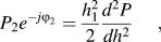 $$![CDATA[$$P_2 e^{ - j\varphi _2 } = {{h_1^2 } \over 2}{{d^2 P} \over {dh^2 }},$$
where P 2 is the amplitude of the second harmonic of load, ϕ 2 is the phase angle between the second harmonic of load and the second harmonic of displacement, and h 1 is the oscillation amplitude of displacement. For a system controlled by CSM, the derivative of the load with respect to the indentation depth is expressed by the following equation:
 $$![CDATA[$${{dP} \over {dh}} = (K - {\rm{\omega }}^2 m)(1 + j\tan (\varphi _1 )),$$
where K is the total harmonic stiffness, ϕ 1 is the phase angle between the first harmonic of load and the first harmonic of displacement, and m is the column mass. To obtain the second derivative, Eq. (19) is derived with respect to the indentation depth in the following way:
 $$![CDATA[$${{d^2 P} \over {dh^2 }} = {{d\left( {{{dP} \over {dh}}} \right)} \over {dK}} \times {{dK} \over {dS}} \times {{dS} \over {dh_{\rm{c}} }} \times {{dh_{\rm{c}} } \over {dh}}.$$
The first term is computed by deriving Eq. (19) with respect to K and supposing the phase angle to be constant. The second term is computed by deriving the following equation with respect to S:
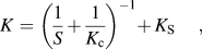 $$![CDATA[$$K = \left( {{1 \over S} + {1 \over {K_{\rm{c}} }}} \right)^{ - 1} + \,K_{\rm{S}} ,$$
where K c is the column stiffness and K s is the support springs stiffness. The third and fourth terms are computed with Eqs. (11) and (13).
Using Eqs. (18) and (20), the reduced elastic contact modulus is thus expressed by the following equation:
 $$![CDATA[$$E_{\rm{c}}^{\prime*} = {{\left| {P_2 } \right|S^2 } \over {{\rm{\alpha }}\tan ({\rm{\theta }})\left( {\sqrt {1 + \tan ^2 (\varphi _1 )} \left( {\left| {h_1 } \right|K} \right)^2 - 2P\left| {P_2 } \right|} \right)}}.$$
The reduced elastic modulus E ′* of the tested material is obtained from Eqs. (15) and (16) and the hardness H from Eq. (14). This new expression is interesting because the indentation depth is not needed to compute the mechanical properties.
We note that the equations derived above are only usable for displacement-controlled systems. In the case of load-controlled systems, the amplitude of the second harmonic of displacement is expressed by the following equation:
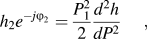 $$![CDATA[$$h_2 e^{ - j\varphi _2 } = {{P_1^2 } \over 2}{{d^2 h} \over {dP^2 }},$$
where h 2 is the amplitude of the second harmonic of displacement. The second derivative of the indentation depth with respect to the load can be expressed in a very simple way as a function of the second derivative of the load with respect to the indentation depth:
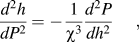 $$![CDATA[$${{d^2 h} \over {dP^2 }} = - {1 \over {{\rm{\chi }}^3 }}{{d^2 P} \over {dh^2 }},$$
where  ${\rm{\chi }} = {{dP} \over {dh}}$. With Eqs. (19), (20), (23), and (24), the expression of the reduced elastic contact modulus is:
 $$![CDATA[$$E_{\rm{c}}^{\prime*} = {{\left| {h_2 } \right|S^2 } \over {{\rm{\alpha }}\tan ({\rm{\theta }})\left( {{{\left( {\left| {P_1 } \right|K} \right)^2 } \over {(K - {\rm{\omega }}^2 m)^3 (1 + \tan ^2 (\varphi _1 ))}} - 2P\left| {h_2 } \right|} \right)}}.$$
The reduced Young modulus is computed with Eq. (16) and the hardness with Eq. (14). In Eq. (25), the amplitude of the second harmonic  $\left| {h_2 } \right|$, the total harmonic stiffness K, the applied load P, the phase angle ϕ 1, and the harmonic load P 1 are measured, the harmonic contact stiffness S is computed, the angular frequency ω is fixed, and the indenter angle θ and the column mass m are known, so it is possible to calculate the reduced elastic contact modulus E c′*, the reduced elastic modulus E ′*, and the hardness H from the detection of the amplitude of the second harmonic, and thus the indentation depth h using Eq. (17). With this new technique, the indentation depth h is not needed, and the uncertainties related to the assessment of the indentation depth, such as the tip defect height estimation, the contact detection, and the thermal drift, are eliminated. Thus, this new technique could be interesting to use for high-temperature tests where reliable indentation depth values are complicated to obtain. It is very important to note that all equations are valid if E c′* is constant during the unloading. With the CSM technique, the unloading curve corresponds to the oscillation amplitude, which is usually set between 0 and 5 nm. If the reduced elastic modulus is quite constant along the indentation depth, the above equations can be used.
V. EXPERIMENTATION
A. Samples and nanoindenter
Experiments were performed on three smooth materials: fused silica, PMMA, and calcite. Fused silica and PMMA samples are supposed to be homogeneous. The calcite was chosen because it exhibits a small indentation size effect (ISE) on the hardness results.Reference Zügner, Marquardt and Zimmermann20
A Nano Indenter SA2® equipped with a DCM head system (Agilent Technologies, Santa Clara, CA) was used. This load-controlled apparatus has high resolution in displacement and force measurement (0.2 pm and 1 nN, respectively). A Berkovich diamond tip was used in the experiments. The equivalent height of the tip defect h 0 was approximately 5 nm. To record the amplitude of the second harmonic of the displacement signal, a second lock-in amplifier (EG&G 7260DSP®, EG&G Technical Services, Norfolk, VA) was attached to the SA2. For more details about the apparatus and materials, please refer to Guillonneau et al.Reference Guillonneau, Kermouche, Bec and Loubet12
B. Indentation procedure
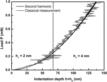
The maximum load applied to the specimens was 5 mN for silica, 0.15 mN for PMMA, and 4.5 mN for calcite. The oscillation amplitude was set to h 1 = 4 nm for fused silica and PMMA samples, whereas for calcite, the oscillation amplitude was gradually increased with the load to avoid loss of information and loss of contact at small penetration depths.Reference Pharr, Strader and Oliver21 More precisely, the oscillation amplitude was h 1 = 2 nm for load between 0 and 0.2 mN and 4 nm for load between 0.2 and 4.5 mN. The oscillation frequency was 97 Hz for fused silica and calcite and 31 Hz for PMMA. The strain rate was  $\dot P$/P = 0.005 s−1 for PMMA and calcite and
 $\dot P$/P = 0.003 s−1 for fused silica.Reference Lucas, Oliver, Pharr, Loubet, Gerberich, Gao, Sundgren and Baker14 Ten indentation tests were realized on each sample. In the following, all the data are mean curves from these 10 tests.
VI. RESULTS AND DISCUSSION
A. Amplitude of the second harmonic
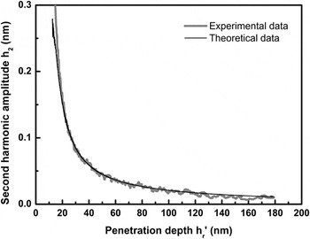
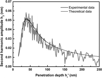
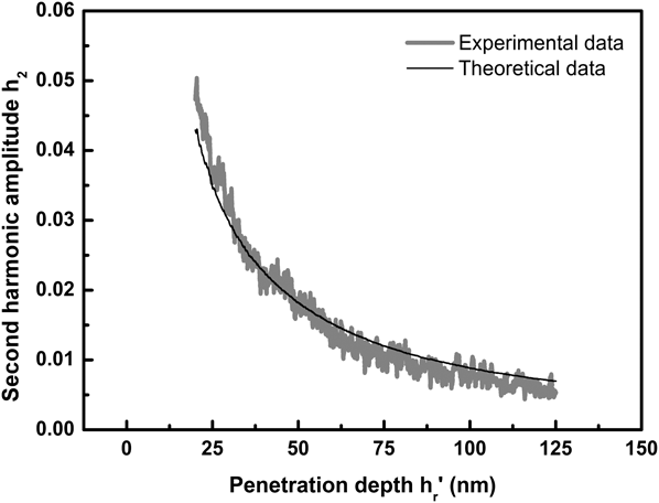
Figures 4, 5, and 6 plot the amplitude of the second harmonic measured on fused silica, PMMA, and calcite, respectively, as a function of the penetration depth h r′. The theoretical curve obtained from Eq. (25) is also plotted (using a reduced elastic modulus for fused silica, PMMA, and calcite of 73,Reference Oliver and Pharr6 5,Reference Guillonneau, Kermouche, Bec and Loubet12 and 77 GPa,Reference Broz, Cook and Whitney22 respectively). The agreement between experimental data and theoretical data is very satisfactory. Furthermore, experimental values are in good agreement with theoretical values for penetration depths between 25 and 100 nm, so mechanical properties will also be accurate in this range of penetration depths.
Amplitude of the second harmonic of displacement versus penetration depth for fused silica: experimental and theoretical curves.

Amplitude of the second harmonic of displacement versus penetration depth for PMMA: experimental and theoretical curves.

Amplitude of the second harmonic of displacement versus penetration depth for calcite: experimental and theoretical curves.
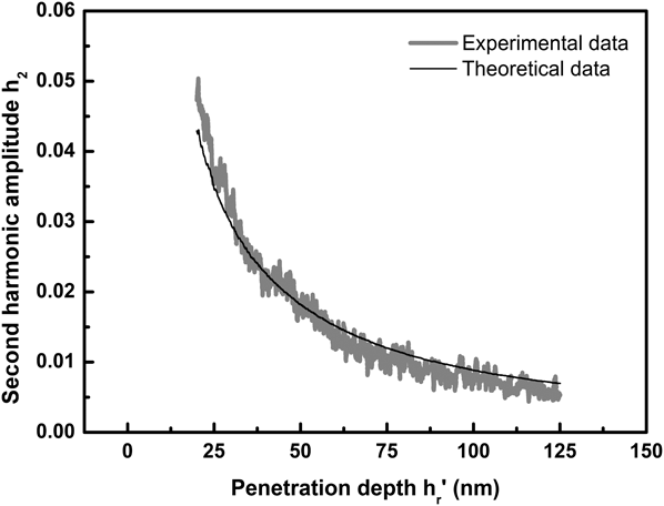
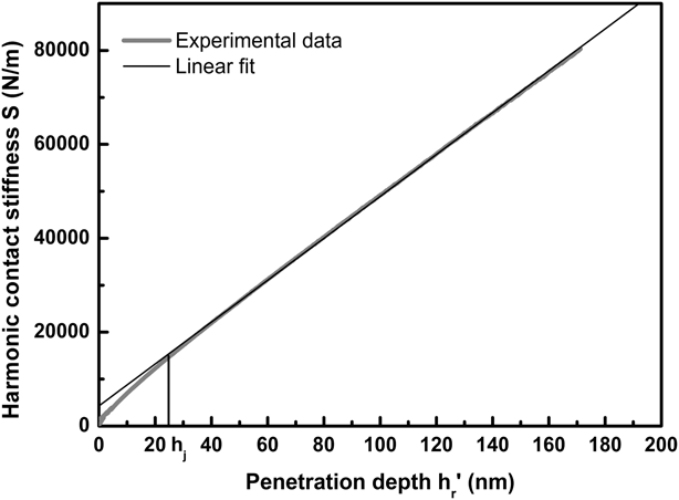
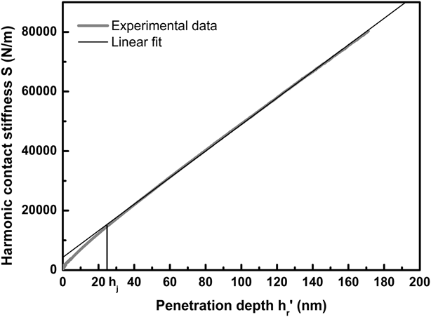
In the case of the fused silica sample (Fig. 4), experimental and theoretical values differ for penetrations depths lower than 25 nm. It can be explained by the geometrical imperfection of the tip (see Sec. II. B). This can be observed by plotting the harmonic contact stiffness versus the penetration depth, which is expected to vary linearly for a homogeneous material such as fused silica (Fig. 7). Here, the linearity is broken below h j = 25 nm, which is in good agreement with the limit identified in Fig. 4.
Harmonic contact stiffness of fused silica versus penetration depth; h j is the limit from which the harmonic contact stiffness is linear with the penetration depth.
In the case of PMMA (Fig. 5), the amplitude of the second harmonic at small penetration depths (<50 nm) increases before decreasing for larger penetration depths. This is caused by the CSM system, which is in transitory mode at the beginning of the test (i.e., the amplitude of the first harmonic is not stabilized). Note that, in the stabilized regime, the amplitude of the second harmonic decreases with the indentation depth. That is why this method is accurate only for small penetration depths; at larger penetration depths, the noise becomes more and more influent.
B. Mechanical properties
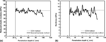
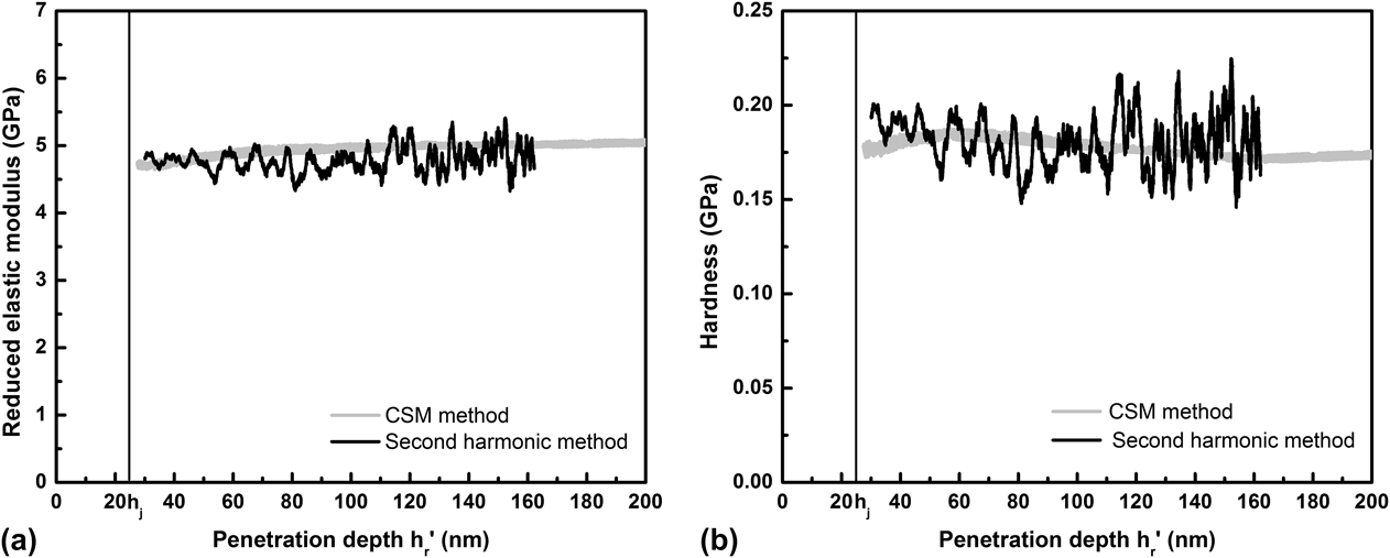
The reduced elastic modulus E ′* and the hardness H of fused silica and PMMA versus the penetration depth are plotted respectively in Figs. 8 and 9. The mechanical properties are computed both from the detection of the amplitude of the second harmonic and from the classical CSM method. The results are similar for both methods, except that the standard deviation is higher in the case of the second harmonic method. This is not surprising because of the low values of the second harmonic amplitude. To solve this problem, it would be interesting to be able to increase automatically the oscillation amplitude with the penetration depth to get an accurate value of the amplitude of the second harmonic during the whole test. Unfortunately, it is not possible with existing devices.
(a) Reduced elastic modulus and (b) hardness versus penetration depth for fused silica.

(a) Reduced elastic modulus and (b) hardness versus penetration depth for PMMA.

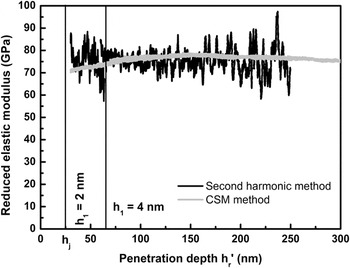
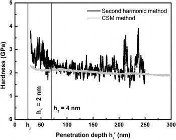
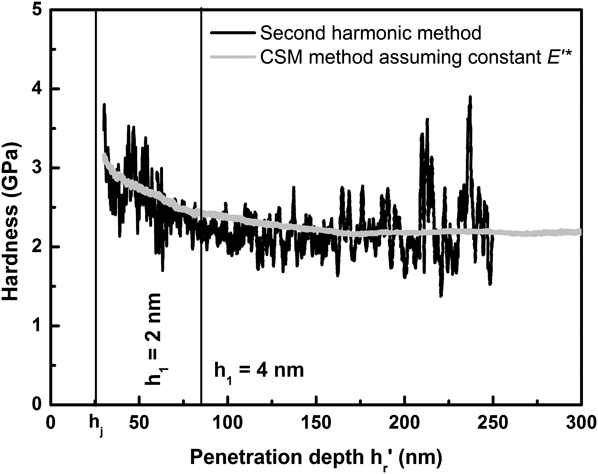
Figures 10 and 11 plot the reduced elastic modulus and the hardness of calcite, respectively, versus the penetration depth. As explained before, the oscillation amplitude was manually increased during the test to get a more precise second harmonic signal. More precisely, for penetration depths between 30 and 70 nm, the oscillation amplitude h 1 was 2 nm, and for higher penetration depths, the oscillation amplitude h 1 was 4 nm. For penetration depths higher than 75 nm approximately, the mechanical properties computed with the two methods are similar, except that the standard deviation is higher in the case of the second harmonic method, as previously observed for fused silica and PMMA.
Reduced elastic modulus versus penetration depth for calcite: second harmonic method versus classical CSM method.

Hardness versus penetration depth for calcite (material expected to exhibit an ISE in hardness): second harmonic method versus classical CSM method.

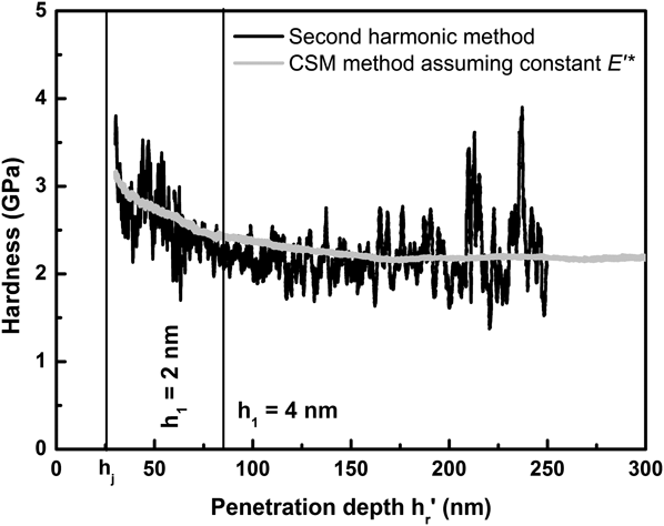
At small penetration depths, the hardness computed with the two methods is slightly different. The ISE makes the hardness of calcite decrease during the first nanometers of penetration, but this decrease appears to be different with the two methods. This could be explained by noting that the reduced elastic modulus is constant with the second harmonic method, whereas it slightly increases with the classical CSM method until it reaches a constant value (around 76 GPa). This apparent increase in elastic modulus in the first nanometers may be caused by uncertainties related to the indentation depth calculation. Calcite is supposed to have a constant reduced elastic modulus, which is what is obtained with the second harmonic method. To go further, we computed the hardness from the CSM method using Eqs. (1) and (2) and assuming a constant elastic modulus (76 GPa). As shown in Fig. 12, when assuming a constant elastic modulus, the hardness curve obtained through the CSM method is very close to hardness values obtained with the second harmonic method. This points to the influence of the uncertainties related to classical CSM methods, which could be removed thanks to the second harmonic method.
Hardness versus penetration depth for calcite assuming a constant reduced elastic modulus value in the calculation of the hardness with the CSM method.
The above analysis shows that the hardness values obtained with the two methods are similar for high penetration depths, and the results are more precise with the second harmonic method for penetration depths between 25 and 100 nm. The obtained mechanical properties are close to literature values.Reference Zügner, Marquardt and Zimmermann20, Reference Broz, Cook and Whitney22, Reference Whitney, Broz and Cook23 As shown with the calcite sample, mechanical properties for inhomogeneous materials can be determined with the second harmonic method.
C. Indentation depth
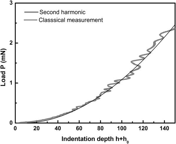
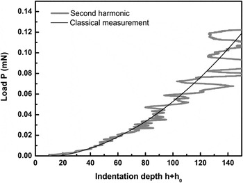
Figures 13, 14, and 15 plot the load–indentation depth curves for fused silica, PMMA, and calcite, respectively. The indentation depth was computed using Eq. (17). It is in very good agreement with the classical indentation depth. The indentation depth is obviously more accurate at small penetration depths because of the higher quality of the second harmonic signal. This indicates that the indentation depth can be computed without using any measurement. This is very promising because it removes the problems related to thermal drift. For instance, this technique could be useful for high-temperature tests where thermal drift is of primary importance.Reference Schuh, Packard and Lund24
Fused silica load–displacement curve obtained with displacement measurement and second harmonic method.
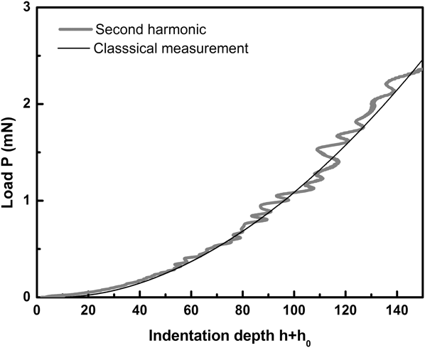
PMMA load–displacement curve obtained with displacement measurement and second harmonic method.

Calcite load–displacement curve obtained with displacement measurement and second harmonic method.

D. Limitation of the technique
The standard deviation is important with the curves obtained from the second harmonic method. This is caused by the noise in the recorded signal because the nanoindenter is not designed to record second harmonic amplitude. As shown in Figs. 4–6, the amplitude of the second harmonic decreases with the penetration depth, so the noise is more and more important. That is why the mechanical properties and the indentation depth are more accurate at small penetration depths. To increase the signal/noise ratio, the oscillation amplitude h 1 should be increased with the penetration depth. Nevertheless, the oscillation amplitude has to be low enough to avoid losing contact between the tip and the sample.Reference Pharr, Strader and Oliver21 Thus, to obtain accurate results, the oscillation amplitude has to be carefully chosen. The second limit is the curvature of the unloading curve. For near fully plastic materials like aluminum, which exhibits a quasilinear unloading curve, the second harmonic signal is too small, so the present method cannot be used.
VII. CONCLUSIONS
In this paper, a new technique based on the detection of the amplitude of the second harmonic of displacement signal has been proposed. With this new method, the reduced elastic modulus and the hardness of materials can be calculated. The obtained expressions do not depend on the indentation depth, so uncertainties related to the displacement measurement, especially at small penetration depths, are eliminated. Furthermore, the indentation depth can be obtained without any use of displacement measurement. This technique can be used for any materials with constant Young modulus. The experimental tests show that the material mechanical properties of fused silica and PMMA can be computed with precision at penetration depths between 25 and 100 nm, which is more difficult with classical tests because the uncertainties related to the indentation depth calculation are very influent in this penetration range. The tests realized on calcite show that the technique can be applied to materials exhibiting ISE, and that the hardness measured with second harmonic method is more precise. In the last part, the indentation depth was computed from second harmonic method. The results obtained with this technique are close to the indentation depth as classically measured. This innovative technique will be interesting for high-temperature tests. Current apparatus, however, are not designed to record precisely the second harmonic, inducing scattering on the results. We expect that future developments will include such type of measurement.