1 Introduction
In coastal areas around the world, breakwaters are commonly used to create a safe wave environment along the coastlines. These structures, also known as wave attenuators, play a crucial role in reducing wave action in inshore waters and in providing secure harbourage. Among several structures, rectangular breakwaters have been extensively studied due to their simple geometry and their effectiveness for shorter waves [Reference Dai, Wang, Utsunomiya and Duan9]. To enhance the efficiency of rectangular structures, researchers have introduced wave-dissipating components, such as protruding plates or wave screens, which can be placed at various locations on the breakwater. Typically, either a single screen extends from the middle, or two screens are added to each edge, both of which have been shown to significantly increase energy dissipation [Reference Deng, Wang, Zhao and Huang11, Reference Koutandos, Prinos and Gironella21]. In real-world applications, concrete floating attenuators are successfully implemented in offshore locations, such as those found in Brooklyn Bridge Park, showcasing their practical use in mitigating wave impact and ensuring safe docking areas.
The present study proposes two rectangular breakwater designs: floating and bottom-fixed, both incorporating two vertical thin porous plates on each side to form a floating
 $\boldsymbol {\sqcap }$
-shaped and bottom-fixed inverted
 $\boldsymbol {\sqcap }$
-shaped breakwater, respectively. Therefore, it is essential to review previous studies on both rectangular breakwaters and vertical porous barriers. In the context of rectangular structures, Mei and Black [Reference Mei and Black27] and Black et al. [Reference Black, Mei and Bray4] introduced a variational formulation for these rigid structures, either placed on the water’s surface or the seabed. Later, Mandal and Kanoria [Reference Mandal and Kanoria26] employed the multi-term Galerkin technique to analyse wave interaction with thick rigid barriers of various configurations in finite water domains. Soylemez and Goren [Reference Söylemez and Gören38] further proposed a simpler linear analytical solution for the first-order wave-diffraction potential, and the associated reflection, transmission and force coefficients for a rectangular barrier fixed at the free surface or fixed on the seabed in finite-depth water.
The wave-attenuating capability is significantly enhanced by introducing porosity into the protruding plates, which offers an effective alternative to rigid structures and creating calm water zones around the structure [Reference Chwang and Chan8]. The most commonly applied model for wave-induced flow in porous media is that developed by Sollitt and Cross [Reference Sollitt and Cross37]. This model accounts for wave energy dissipation within a porous medium through a linearized friction term, evaluated using an iterative approach. Chwang [Reference Chwang7] developed a porous-wavemaker theory to analyse small-amplitude surface waves on finite depth water, produced by the horizontal oscillation of a porous vertical plate. Subsequently, Lee and Chwang [Reference Lee and Chwang22] applied the least squares method to examine the scattering and generation of water waves by vertical permeable barriers. Several notable studies [Reference Behera, Mandal and Sahoo2, Reference Behera and Ng3, Reference Khan and Behera18, Reference Khan, Behera, Sahoo and Neelamani19, Reference Venkateswarlu, Panduranga, Vijay and Behera39] in the literature on porous structures have explored wave trapping by composite structures near rigid walls. The structural porosity in these studies plays a crucial role in dissipating wave energy. In addition to vertical porous plates, some key works ([Reference Guo, Mohapatra and Soares15, Reference Mohapatra, Sahoo and Soares28–Reference Mohapatra and Soares30] and the literature cited therein) on horizontal flexible porous plates have been performed under the assumption of small amplitude wave theory.
The study of wave scattering by rectangular breakwaters has gained increasing interest as new configurations outperform conventional, simpler designs. These enhanced structures incorporate vertical thin protruding plates with permeable or impermeable features, forming
 $\boldsymbol {\sqcap }$
-shaped or inverted
 $\boldsymbol {\sqcap }$
-shaped structures when added either downward or upward. Gesraha [Reference Gesraha14] introduced the floating
 $\boldsymbol {\sqcap }$
-shaped structure and showed that this configuration reduced both the transmission coefficient and hydrodynamic responses compared with a rectangular structure of identical mass. Later, Ruol et al. [Reference Ruol, Martinelli and Pezzutto32] derived a useful formula to estimate the wave transmission coefficient for
 $\boldsymbol {\sqcap }$
-shaped floating breakwaters, noting that the formula was not applicable for high-wave conditions. Recently, Fouladi et al. [Reference Fouladi, Bahmanpouri, Rezazadeh, Kollolemad, Mashayekhi and Viccione13] applied the Scaled Boundary Finite Element Method to solve the water wave and
 $\boldsymbol {\sqcap }$
-shaped floating breakwater interaction. Such a type of
 $\boldsymbol {\sqcap }$
-shaped floating structure found at SF MARINA in Skärhamn, Sweden, consists of four sections of the structure connected in series, and anchored using chains and anchors [Reference Lundström24]. Apart from the floating structure, few studies highlighted that adding thin plates to a bottom-fixed rectangular structure significantly enhances its performance compared with a standard rectangular configuration. A recent study by Singh et al. [Reference Singh, Kaligatla and Mandal36] revealed that incorporating upward-facing plates into a bottom-fixed rectangular breakwater substantially improves wave scattering. Very recently, Sharma et al. [Reference Sharma, Sarkar and De35] employed the multi-term Galerkin technique to demonstrate the wave scattering by a pair of inverted
 $\boldsymbol {\sqcap }$
-shaped breakwaters. However, few studies have explored the impact of adding permeable plates to both sides of a rectangular breakwater. Notably, Cho [Reference Cho6] demonstrated that proper porosity and deeper immersion of vertical plates could significantly reduce the transmission coefficient. Motivated by this work, a semi-analytical method is used to study oblique wave interaction with
 $\boldsymbol {\sqcap }$
-shaped floating and inverted bottom-fixed breakwaters with porous plates, assuming linearized water wave theory. As such a type of breakwater is relatively unexplored, it presents an opportunity to investigate the impact of adding two porous side plates on the performance of a rectangular breakwater. The multi-term Galerkin method provides a highly accurate and rapidly converging solution, effectively capturing the singular behaviour of velocity near submerged edges. This study uses the multi-term Galerkin method to analyse wave scattering and evaluate the performance of such breakwaters with high accuracy. This adds some sort of novelty and significant contribution to the literature on water waves. To do this, we simplify the physical scenario into a boundary value problem and reformulate it into Fredholm-type integral equations using the method of eigenfunction expansion. The integral equations are subsequently solved using the multi-term Galerkin approximation method, where Chebyshev polynomials are chosen as the basis functions and with suitable weight. The selection of basis functions effectively handles the square-root singularities at both the sharp and submerged ends of the models. Convergence analysis is performed for both breakwater types, and the method’s accuracy is validated against existing results. A parametric study on the scattering coefficient evaluates breakwater effectiveness, while free surface elevation and horizontal drift force analyses assess the performance of both structures.
2 Theoretical formulation
The Cartesian coordinate system
 $(x, y, z)$
is employed, where the
 $xz$
-plane represents the mean free surface and the y-axis points vertically downwards. The study considers a
 $\boldsymbol {\sqcap }$
-shaped configuration composed of thin porous plates and a thick rigid block in a fluid domain of finite depth H. The breakwater configuration can either be a floating structure or a bottom-fixed inverted structure, with two porous plates positioned at
 $x=-w_1$
and
 $x=w_2$
. The cross-sectional representation of this configuration, shown in Figure 1, illustrates how the entire domain is divided into three distinct sub-regions,
 $R_j~(j=1,2,3)$
, based on the structural geometry.
Problem sketch for (a) floating
 $\boldsymbol {\sqcap }$
-shaped and (b) bottom-fixed inverted
 $\boldsymbol {\sqcap }$
-shaped breakwater.

Under the assumptions that the fluid is incompressible and inviscid, a scalar velocity potential can be defined as
 $\Phi (x,y,z,t) = \mbox {Re}[\phi (x,y)e^{\mathrm {{i}(\nu z-\omega t)}}]$
, where
 $\mbox {Re}[~]$
represents the real part of the complex expression. The term
 $\nu ={k}_{0}\sin \theta $
defines the horizontal wavenumber component, where
 ${k}_{0}$
is the wavenumber of the incident wave,
 $\theta $
is the angle of incidence and the angular frequency is denoted by
 $\omega $
. Since the breakwater extends along the z-direction, the solution exhibits periodicity in that direction. Consequently, the interface between different regions can be analysed using Snell’s law [Reference Kirby and Dalrymple20]. Within the entire fluid domain, the velocity potentials must satisfy the Laplace equation. However, due to the periodic variation in the z-direction, the governing equation can be reformulated as the modified Helmholtz equation [Reference Mandal and Chakrabarti25]:
 $$ \begin{align*} \bigg(\frac{\partial^2}{\partial x^2}+\frac{\partial^2}{\partial y^2}-\nu^2\bigg)\phi(x,y)=0 \quad\text{for all } (x, y)\in(-\infty, \infty) \times (0, H), \end{align*} $$
where
 $\phi (x,y)$
represents the spatial part of the complex velocity potential.
By combining the kinematic and dynamic boundary conditions under the principles of linear water-wave theory, the boundary condition at the mean free surface can be expressed as
 $$ \begin{align*} \bigg(g\frac{\partial}{\partial y}+\omega^2\bigg)\phi(x,y)\bigg|_{y = 0}=0, \begin{cases} x\in \mathbb{R}\setminus (-w_1, w_2)&\mbox{for~floating~structure},\\ x\in \mathbb{R}&\mbox{for~bottom-fixed~structure}, \end{cases} \end{align*} $$
where g and
 $\mathbb {R}$
have their usual meaning.
The seabed and the horizontal segment of the
 $\boldsymbol {\sqcap }$
-shaped configuration are considered rigid and impermeable, satisfying the zero normal velocity condition, expressed as follows:
 $$ \begin{align*} \frac{\partial \phi(x,y)}{\partial y}\bigg|_{y = H}=0, \begin{cases} x\in \mathbb{R}&\mbox{for~floating~structure},\\ x\in \mathbb{R}\setminus (-w_1, w_2)&\mbox{for~bottom-fixed~structure}, \end{cases} \end{align*} $$
and
 $$ \begin{align*} \frac{\partial \phi(x,y)}{\partial y}\bigg|_{y = d}=0,~x\in (-w_1, w_2)\quad\mbox{for~both~structures}. \end{align*} $$
The boundary condition for the rigid thick block and the thin porous plates of the
 $\boldsymbol {\sqcap }$
-shaped structure is defined as
 $$ \begin{align} \frac{\partial \phi(x,y)}{\partial x}\bigg|_{x = -w_1,w_2}=0, \begin{cases} y\in (0, d)&\mbox{for~floating~structure},\\ y\in (d, H)&\mbox{for~bottom-fixed~structure}, \end{cases} \end{align} $$
and
 $$ \begin{align} \begin{aligned} \frac{\partial \phi(x,y)}{\partial x}\bigg|_{x = -w_1}&= -{i}k_0 G_1\{\phi(-w_1+0,y)-\phi(-w_1-0,y)\}~\\ &\quad \mbox{on} \begin{cases} y\in (d, h_1)&\mbox{for~floating~structure},\\ y\in (h_1, d)&\mbox{for~bottom-fixed~structure}; \end{cases} \end{aligned} \end{align} $$
 $$ \begin{align} \begin{aligned} \frac{\partial \phi(x,y)}{\partial x}\bigg|_{x = w_2}&= -{i}k_0 G_2\{\phi(w_2+0,y)-\phi(w_2-0,y)\}~\\ &\quad \mbox{on} \begin{cases} y\in (d, h_2)&\mbox{for~floating~structure},\\ y\in (h_2, d)&\mbox{for~bottom-fixed~structure}; \end{cases} \end{aligned} \end{align} $$
where
 $G_1$
and
 $G_2$
are the complex porous effect parameters of front and rear plates, respectively, as defined by Yu and Chwang [Reference Yu and Chwang40]. The real components,
 $\mbox {Re}[G_1]$
and
 $\mbox {Re}[G_2]$
, represent the resistance offered by the porous material to seepage flow, whereas the imaginary components,
 $\mbox {Im}[G_1]$
and
 $\mbox {Im}[G_2]$
, correspond to the inertial influence of the fluid moving through the porous medium. Throughout the fluid domain, the velocity potential remains bounded, except at the submerged sharp edges of the
 $\boldsymbol {\sqcap }$
-shaped structure. The boundary conditions at these edges are given as follows [Reference Mandal and Chakrabarti25]:
 $$ \begin{align} |\nabla\phi|=O(r^{-1/2})\quad\mbox{as } \textit{r}\rightarrow 0, \end{align} $$
where r=
 ${((x+w_1)^2+(y-h_1)^2)}^{1/2}$
for the front plate and r=
 ${((x-w_2)^2+(y-h_2)^2)}^{1/2}$
for the rear plate.
Given that the incident wave propagates along the x-axis from negative infinity, the far-field condition is expressed as follows:
 $$ \begin{align*} \phi(x,y)\sim \begin{cases} \phi^{\mathrm{inc}}(x,y)+R\phi^{\mathrm{inc}}(-x,y) &\mbox{as } x\rightarrow -\infty,\\ T \phi^{\mathrm{inc}}(x,y) &\mbox{as } x\rightarrow \infty, \end{cases} \end{align*} $$
where the incident potential,
 $\phi ^{\mathrm {inc}}(x,y)$
, is expressed as
 $$ \begin{align*} \phi^{\mathrm{inc}}(x,y)= \frac{\cosh {k}_{0}(H-y)}{\cosh {k}_{0}H}e^{{i}\mu(x+w_1)} \end{align*} $$
with
 $\mu ={k}_{0}\cos \theta $
.
3 Analytical solution
The mathematical representation of the velocity potential
 $\phi (x,y)$
for the three sub-regions, namely
 $R_1,R_2,R_3$
, created in the fluid domain by the
 $\boldsymbol {\sqcap }$
-shaped breakwater designs (both floating and bottom fixed) have been obtained by using Havelock’s expansion formulae [Reference Mandal and Kanoria26].
In the sub-region,
 $R_1 = \{(x,y)\mid -\infty <x<-w_1, 0<y<H\}$
, the velocity potential comprises contributions from the incident and reflected waves. The mathematical expressions for
 $\phi (x,y)$
corresponding to both breakwater configurations are given as
 $$ \begin{align} \phi(x,y)=\{e^{{i}\mu(x+w_1)}+V_1e^{-{i}\mu(x+w_1)}\}\frac{\cosh {k}_0(H-y)}{\cosh {k}_0H}+\sum\limits_{n=1}^{\infty}{A}_{n} e^{{s}_{n}(x+w_1)}\frac{\cos {k}_n(H-y)}{\cos {k}_nH}, \end{align} $$
where
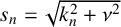 $s_{n}=\sqrt {{k}_{n}^{2}+\nu ^{2}}$
,
 $A_{n}$
values
 $(n=1,2,\ldots )$
represent the unknown expansion coefficients and the constant
 $V_{1}$
relates to the reflection coefficient R through the expression [Reference Evans and Porter12, Reference Sarkar, De and Gayen33, Reference Sarkar, Roy and De34],
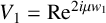 $V_1=\mbox {Re}^{2{i}\mu w_1}$
.
In the sub-region,
 $R_2=\{(x,y)\mid -w_1<x<w_2, d<y<H\}$
for floating structure, or
 $R_{2}=\{(x,y)\mid -w_1<x<w_2, 0<y<d\}$
for bottom-fixed structure, the velocity potential
 $\phi (x,y)$
is expressed as a series of eigenfunctions given by: for the floating structure,
 $$ \begin{align} \phi(x,y)&=({B}_{0} \cosh \lbrace\nu (x+w_1)\rbrace+{C}_{0} \sinh \lbrace\nu (x-w_2)\rbrace) \nonumber\\&\quad +\sum_{n=1}^{\infty}({B}_{n} \cosh \lbrace\xi_n (x+w_1)\rbrace+{C}_{n} \sinh \lbrace\xi_n (x-w_2)\rbrace) \cos\bigg\lbrace \frac{n\pi (y-d)}{H-d}\bigg\rbrace; \end{align} $$
and for the bottom-fixed structure,
 $$ \begin{align} \begin{aligned} &\phi(x,y)=({B}_{0} \cos \lbrace({\alpha}_{0}^{2}-\nu^2)^{{1}/{2}} (x+w_1)\rbrace+{C}_{0} \sin \lbrace({\alpha}_{0}^{2}-\nu^2)^{{1}/{2}} (x-w_2)\rbrace)\frac{\cosh {\alpha}_0(d-y)}{\cosh {\alpha}_0d} \\ &\quad+\sum_{n=1}^{\infty}({B}_{n} \cosh \lbrace({\alpha}_{n}^{2}+\nu^2)^{{1}/{2}} (x+w_1)\rbrace+{C}_{n} \sinh \lbrace({\alpha}_{n}^{2}+\nu^2)^{{1}/{2}} (x-w_2)\rbrace) \cos {\alpha}_n(d-y),\\ \end{aligned} \end{align} $$
where
 $\xi _n=\sqrt {({n\pi }{(H-d)})^2+\nu ^2}~(n=1,2,\ldots )$
. Additionally,
 ${B}_{n}$
terms and
 ${C}_{n}$
terms
 $(n=0,1,2,\ldots )$
are unknown constants.
In the sub-region
 $R_3=\{(x,y)\mid w_2<x<\infty ,0<y<H\}$
, the complex potential function accounts for the effects of transmitted waves. Consequently, the formal expressions for
 $\phi (x,y)$
in both breakwater models are provided as
 $$ \begin{align} \begin{aligned} \phi(x,y)=V_{2}e^{{i}\mu(x-w_2)}\frac{\cosh {k}_0(H-y)}{\cosh {k}_0H}+\sum_{n=1}^{\infty}E_{n}e^{-s_{n}(x-w_2)}\frac{\cos {k}_n(H-y)}{\cos {k}_nH}, \end{aligned} \end{align} $$
where
 $E_{n}~(n=1,2,\ldots )$
denotes the unknown expansion coefficients, while the constant
 $V_{2}$
is connected to the transmission coefficient T through the relation [Reference Evans and Porter12, Reference Sarkar, De and Gayen33, Reference Sarkar, Roy and De34],
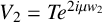 $V_2 = T e^{2{i} \mu w_2}$
. The above-mentioned wavenumbers
 $\pm k_{0}$
and
 $\pm \alpha _{0}$
(representing progressive waves) satisfy the following dispersion relation:
 $$ \begin{align*} \tanh{ph}=\frac{K}{p} \begin{cases} p=k \mbox{~and~} h=H \quad\mbox{for both breakwater in sub-regions } R_1 \mbox{ and } R_3,\\ p=\alpha \mbox{~and~} h=d \quad\mbox{for bottom-fixed breakwater in sub-regions } R_2, \end{cases} \end{align*} $$
where
 $K={\omega ^2}/{g}$
.
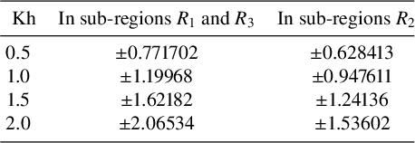
Table 1 illustrates some numerical examples of roots of the above dispersion relation.
Roots of the dispersion relation.

Also, the wavenumbers
 $\pm {i}k_{r}$
and
 $\pm {i}\alpha _{r}~(r=1,2,\ldots )$
(representing evanescent modes) are solutions of the transcendental equation
 $$ \begin{align*} \tan{\gamma h}=-\frac{K}{\gamma} \begin{cases} \gamma=k \mbox{~and~} h=H \quad\mbox{for both breakwater in sub-regions } R_1 \mbox{ and } R_3,\\ \gamma=\alpha \mbox{~and~} h=d \quad\mbox{for bottom-fixed breakwater in sub-regions } R_2. \end{cases} \end{align*} $$
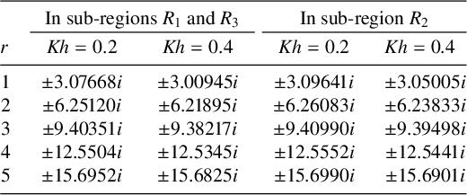
Roots of the transcendental equation.

Similarly, Table 2 illustrates some numerical examples of roots of the above transcendental equation. Let us define the horizontal component of fluid velocity for both breakwater structures as
 $$ \begin{align} f_1(y)&=\frac{\partial \phi(x,y)}{\partial x}\bigg|_{x = -w_1\pm 0},\quad y\in(0,H), \end{align} $$
 $$ \begin{align} f_2(y)&=\frac{\partial \phi(x,y)}{\partial x}\bigg|_{x = w_2\pm 0},\quad y\in(0,H). \end{align} $$
Based on the conditions in equations (2.1) and (2.2), the following equations can be derived:
for the floating structure,
 $$ \begin{align*} f_1(y)&= \begin{cases} 0,~y\in (0,d),\\ -{i}k_0 G_1\{\phi(-w_1+0,y)-\phi(-w_1-0,y)\},\quad y\in (d, h_1), \end{cases} \\ f_2(y)&= \begin{cases} 0,~y\in (0,d),\\ -{i}k_0 G_2\{\phi(w_2+0,y)-\phi(w_2-0,y)\},\quad y\in (d, h_2); \end{cases} \end{align*} $$
and for the bottom-fixed structure,
 $$ \begin{align*} f_1(y)&= \begin{cases} 0,~y\in (d,H),\\ -{i}k_0 G_1\{\phi(-w_1+0,y)-\phi(-w_1-0,y)\}, \quad y\in (h_1, d), \end{cases} \\ f_2(y)&= \begin{cases} 0,~y\in (d, H),\\ -{i}k_0 G_2\{\phi(w_2+0,y)-\phi(w_2-0,y)\},\quad y\in (h_2, d). \end{cases} \end{align*} $$
As a result of the edge conditions outlined in equation (2.3), the functions
 $f_j(y)~(j=1,2)$
display singularities close to the submerged sharp edges. According to Mandal and Chakrabarti [Reference Mandal and Chakrabarti25], the singularity behaviour at the submerged edges of the thin plates in the
 $\boldsymbol {\sqcap }$
-shaped breakwater follows a form proportional to
 $|y - h_j|^{-1/2} (j=1,2)$
.
Substituting the expansions of
 $\phi (x,y)$
from equations (3.1)–(3.3) into equation (3.4) and using Havelock’s inversion formula [Reference Havelock16], all constants associated with
 $\phi (x,y)$
in different sub-regions can be expressed as integrals involving
 $f_{j}(y)~(j=1,2)$
. Additionally, the continuity of the velocity potential across the gap below or above the thin porous plates must be preserved. This continuity condition results in the following coupled integral equations:
 $$ \begin{align*} \sum_{j=1}^{2} \int_{l} f_j(u)\mathcal{M}_{ij}(y,u)\, du = \mathcal{K}_{i}(y),\quad y\in \Omega_i~(i=1,2), \end{align*} $$
where
 $l \equiv (d, H)$
and
 $\Omega _i \equiv (h_i, H)~(i=1,2)$
for the floating
 $\boldsymbol {\sqcap }$
-shaped structure, while
 $l \equiv (0, d)$
and
 $\Omega _i \equiv (0, h_i)~(i=1,2)$
for the bottom-fixed
 $\boldsymbol {\sqcap }$
-shaped structure. The definitions of the functions
 $\mathcal {M}_{ij}(y,u)$
and
 $\mathcal {K}_{i}(y)$
 $(i,j=1,2)$
are given as follows.
For the floating structure,
 $$ \begin{align*} \mathcal{M}_{11}(y,u)&= -\frac{\coth\lbrace\nu(w_1+w_2)\rbrace}{\nu(H-d)} \nonumber\\[4pt]&\quad -\sum\limits_{n=1}^{\infty}\frac{2\coth \lbrace\xi_n(w_1+w_2)\rbrace\cos \lbrace\frac{n\pi(y-d)}{(H-d)}\rbrace \cos \lbrace\frac{n\pi(u-d)}{(H-d)}\rbrace}{\xi_n(H-d)}\\[4pt]&\quad-\sum\limits_{n=1}^{\infty}\frac{4k_{n}\cos k_{n}(H-y)\cos k_{n}(H-u)}{s_{n}(2k_{n}H+\sin 2k_{n}H)},\nonumber\\[-2pc] \end{align*} $$
 $$ \begin{align*} \mathcal{M}_{12}(y,u)&= \frac{\operatorname{\mathrm{csch}}\lbrace\nu(w_1+w_2)\rbrace}{\nu(H-d)}\nonumber\\[4pt]&\quad +\sum\limits_{n=1}^{\infty}\frac{2\operatorname{\mathrm{csch}} \lbrace\xi_n(w_1+w_2)\rbrace\cos \lbrace\frac{n\pi(y-d)}{(H-d)}\rbrace \cos \lbrace\frac{n\pi(u-d)}{(H-d)}\rbrace}{\xi_n(H-d)}; \end{align*} $$
and for the bottom-fixed structure,
 $$ \begin{align*} \mathcal{M}_{11}(y,u)&= \frac{4\alpha_{0}\cot\lbrace({\alpha}_{0}^{2}-\nu^2)^{{1}/{2}} (w_1+w_2)\rbrace\cosh \alpha_{0}(d-y)\cosh \alpha_{0}(d-u)}{({\alpha}_{0}^{2}-\nu^2)^{{1}/{2}}(2\alpha_{0}d+\sinh 2\alpha_{0}d)}\nonumber\\[4pt]&\quad -\sum\limits_{n=1}^{\infty}\frac{4k_{n}\cos k_{n}(H-y)\cos k_{n}(H-u)}{s_{n}(2k_{n}H+\sin 2k_{n}H)}\nonumber\\[4pt]&\quad -\sum\limits_{n=1}^{\infty}\frac{4\alpha_{n}\coth\lbrace({\alpha}_{n}^{2}+\nu^2)^{{1}/{2}} (w_1+w_2)\rbrace\cos \alpha_{n}(d-y)\cos \alpha_{n}(d-u)}{({\alpha}_{n}^{2}+\nu^2)^{{1}/{2}}(2\alpha_{n}d+\sin 2\alpha_{n}d)},\nonumber\\[-1.8pc] \end{align*} $$
 $$ \begin{align*} \mathcal{M}_{12}(y,u)&= -\frac{4\alpha_{0}\csc\lbrace({\alpha}_{0}^{2}-\nu^2)^{{1}/{2}} (w_1+w_2)\rbrace\cosh \alpha_{0}(d-y)\cosh \alpha_{0}(d-u)}{({\alpha}_{0}^{2}-\nu^2)^{{1}/{2}}(2\alpha_{0}d+\sinh 2\alpha_{0}d)}\nonumber\\[4pt]&\quad +\sum\limits_{n=1}^{\infty}\frac{4\alpha_{n}\operatorname{\mathrm{csch}}\lbrace({\alpha}_{n}^{2}+\nu^2)^{{1}/{2}} (w_1+w_2)\rbrace\cos \alpha_{n}(d-y)\cos \alpha_{n}(d-u)}{({\alpha}_{n}^{2}+\nu^2)^{{1}/{2}}(2\alpha_{n}d+\sin 2\alpha_{n}d)},\nonumber\\[-1.8pc] \end{align*} $$
 $$ \begin{align*} \mathcal{M}_{21}(y,u)=\mathcal{M}_{12}(y,u),~\mathcal{M}_{22}(y,u)=\mathcal{M}_{11}(y,u) \quad (\mbox{for~both~structures}) \end{align*} $$
 $$ \begin{align*} \mathcal{K}_{1}(y)&=\frac{\cosh {k}_0(H-y)}{\cosh {k}_0H}(1+V_1),\nonumber\\[4pt]\mathcal{K}_{2}(y) &=\frac{\cosh {k}_0(H-y)}{\cosh {k}_0H}(-V_2)\quad (\mbox{for both structures}). \end{align*} $$
Let us now define the following transformation as
 $$ \begin{align} f_{j}(y)=\sum_{i=1}^{2}\mathcal{F}_{ji}(y)({A}_{i}+{B}_{i}), \quad y\in(0,H)~(j=1,2)\end{align} $$
where
 $$ \begin{align} {A}_{1}=1,\quad {A}_{2}=0,\quad {B}_{1}=V_1,\quad {B}_{2}=-V_2. \end{align} $$
By substituting equation (3.6) into equation (3.7), we obtain
 $$ \begin{align} \sum_{j=1}^{2} \int_{l} \bigg\{\sum_{i=1}^{2}\mathcal{F}_{ji}(u)({A}_{i}+{B}_{i})\bigg\}\mathcal{M}_{ij}(y,u)\,du=({A}_{i}+{B}_{i})\mathcal{P}_{i}(y),\quad y\in \Omega_i~(i=1,2), \end{align} $$
where
 $\mathcal {P}_{1}(y)=\mathcal {P}_{2}(y)={\cosh {k}_0(H-y)}/{\cosh {k}_0H}$
.
Using Havelock’s inversion formula, the unknown constants
 $V_1$
and
 $V_2$
are represented in terms of
 $f_{1}(y)$
and
 $f_{2}(y)$
, respectively. Then, by employing equation (3.6), the following equations are obtained:
 $$ \begin{align} (A_j-B_j) W_j Q_j = \sum_{i=1}^{2}S_{ji}(A_i+B_i) \quad (j=1,2), \end{align} $$
where
 $W_1=W_2={{i}\mu }/{k_0}$
,
 $Q_1=Q_2= \{{2k_{0}H+\sinh 2k_{0}H}\}/{4\cosh k_0H}$
and
 $S_{ji}= \int _{l}\mathcal {F}_{ji}(y) \mathcal {P}_j(y)\,dy, \, (i,j=1,2)$
. By reorganizing the terms in equation (3.9), we obtain expression of
 $B_j$
values
 $(j=1,2)$
in terms of
 $A_1$
and
 $A_2$
.
To address the singularity and enhance convergence in numerical computations, the Galerkin approximation method, as described by Evans and Porter [Reference Evans and Porter12], is employed. As a result, the unknown functions
 $\mathcal {F}_{jl}(y)$
are approximated using an
 $(N + 1)$
-term Galerkin expansion, expressed in the following form:
 $$ \begin{align} \mathcal{F}_{jl}(y) \simeq \sum_{n=0}^{N} {a}^{(n)}_{jl}{q}_{j}^{(n)}(y),\quad j,l=1,2. \end{align} $$
In this framework,
 ${a}^{(n)}_{jl}$
signifies the unknown expansion coefficients, whereas
 ${q}_{j}^{(n)}(y)$
denotes the basis functions. These basis functions,
 ${q}_{j}^{(n)}(y)~(j=1,2; n=0,1,2,\ldots ,N)$
, are determined according to the procedure details in [Reference Evans and Porter12].
For the floating structure:
 $$ \begin{align*} & {q}_{j}^{(n)}(y)=\\ &\quad \begin{cases} \dfrac{d}{dy}\bigg[e^{-Ky}\displaystyle\int_{y}^{{h}_{j}}e^{Ku}\dfrac{2(-1)^n\lbrace({h}_{j}-d)^{2}-(u-d)^2\rbrace^{{1}/{2}}}{\pi (2n+1) H (h_j-d)}U_{2n}\bigg(\dfrac{u-d}{{h}_{j}-d}\bigg)\,du\bigg]&\mbox{for}~y\in (d, h_j),\\[.3cm] \dfrac{2(-1)^n}{\pi \lbrace(H-{h}_{j})^{2}-(H-u)^2\rbrace^{{1}/{2}}}T_{2n}\bigg(\dfrac{H-u}{H-{h}_{j}}\bigg)&\mbox{for}~y\in (h_j, H); \end{cases} \end{align*} $$
and for the bottom-fixed structure:
 $$ \begin{align*} {q}_{j}^{(n)}(y)= \begin{cases} -\dfrac{d}{dy}\bigg[e^{-Ky}\displaystyle\int_{y}^{{h}_{j}}e^{Ku}\dfrac{2(-1)^n}{\pi \lbrace{h}_{j}^{2}-u^2\rbrace^{{1}/{2}}}T_{2n}\bigg(\dfrac{u}{{h}_{j}}\bigg)\,du\bigg]&\mbox{for}~y\in (0, h_j),\\[.3cm] \dfrac{2(-1)^n \lbrace(d-{h}_{j})^{2}-(d-u)^2\rbrace^{{1}/{2}}}{\pi (2n+1) (d-h_j) d }U_{2n}\bigg(\dfrac{d-u}{d-{h}_{j}}\bigg)&\mbox{for}~y\in (h_j, d); \end{cases} \end{align*} $$
where
 $T_{2n}(x)$
and
 ${U}_{2n}(x)$
denote the even degree Chebyshev polynomials of the first and second kinds, respectively.
Starting with the substitution of
 $\mathcal {F}_{jl}(y)$
from equation (3.10) into equation (3.8), the equation is then multiplied by
 ${q}_{j}^{(m)}(y)$
and integrated over the interval l. This process yields a set of linear algebraic equations that determine the unknown coefficients
 ${a}^{(n)}_{jl}$
for both configurations, as shown as
 $$ \begin{align} \sum_{n=0}^{N}\sum_{j=1}^{2}{a}^{(n)}_{jl} \mathcal{V}^{(pj)}_{mn}=\delta_{pl}\mathcal{W}^{(p)}_{m},\quad p,l=1,2;\quad m=0,1,\ldots,N, \end{align} $$
where
 $\delta _{pl}$
is the Kronecker delta function and for
 $p,j=1,2$
and
 $m,n=0,1,\ldots ,N,$
 $$ \begin{align*} \mathcal{V}^{(pj)}_{mn}&=\int_{l} \bigg\{{q}_{p}^{(m)}(y)\bigg\{\int_{l}\mathcal{M}_{pj}(y,u){q}_{j}^{(n)}(u)\,du\bigg\}\, dy\bigg\},\quad \mathcal{W}^{(p)}_{m}= \int_{\Omega_p}{q}_{p}^{(m)}(y)\mathcal{P}_{p}(y)\,dy. \end{align*} $$
Using the expression of
 $\mathcal {M}_{pj}(y,u)~(p,j=1,2)$
as in equation (3.11), the expressions for
 $\mathcal {V}^{(pj)}_{mn}$
and
 $\mathcal {W}^{(p)}_{m}~(p,j=1,2; m,n=0,1,\ldots ,N)$
are as follows.
For the floating structure:
 $$ \begin{align*} &{V}^{(pp)}_{mn}=\nonumber\\&-\frac{\coth\lbrace\nu(w_1+w_2)\rbrace}{\nu(H-d)} \bigg[\bigg\lbrace\delta_{m0}+\frac{2{i}(-1)^m(h_p-d)k_0G_p}{\pi(2m+1)H}\int_{0}^{1}e^{K(h_p-d)u}(1-u^2)^{{1}/{2}}U_{2m}(u)\,du\bigg\rbrace\nonumber\\&\times \bigg\lbrace\delta_{n0}+\frac{2{i}(-1)^n(h_p-d)k_0G_p}{\pi(2n+1)H} \int_{0}^{1}e^{K(h_p-d)u}(1-u^2)^{{1}/{2}}U_{2n}(u)\,du\bigg\rbrace\bigg]\nonumber\\& -\sum\limits_{r=1}^{\infty}\frac{4k_r}{s_r(2k_rH+\sin2k_rH)} \bigg[\bigg\lbrace J_{2m}\{k_r(H-h_p)\}-\frac{{i}k_{0}G_p}{k_rH}\cos k_r(H-d)J_{2m+1}\{k_r(h_p-d)\}\bigg\rbrace\nonumber\\&\times\bigg\lbrace J_{2n}\{k_r(H-h_p)\}-\frac{{i}k_{0}G_p}{k_rH}\cos k_r(H-d)J_{2n+1}\{k_r(h_p{\kern-1pt}-{\kern-1pt}d)\}\bigg\rbrace\bigg]-{\kern-1pt}\sum\limits_{r=1}^{\infty}\frac{2\coth\lbrace\xi_r(w_1+w_2)\rbrace}{\xi_r(H-d)}\nonumber\\&\times\bigg[\bigg\{\frac{2(-1)^m}{\pi}\int_{0}^{1} \frac{T_{2m}(u)}{(1-u^2)^{{1}/{2}}}\cos\bigg\lbrace r\pi \bigg(1-\frac{H-h_p}{H-d}u\bigg)\bigg\rbrace du +(-1)^p \frac{2{i}(-1)^m(h_p-d)k_{0}G_p}{\pi(2m+1)H} \nonumber\\&\times\bigg(\cos\bigg(\tan^{-1}\bigg(\frac{K(H-d)}{r\pi}\bigg)\bigg)\int_{0}^{1}(1-u^2)^{{1}/{2}}U_{2m}(u)\cos\bigg(r\pi u-\tan^{-1} \bigg(\frac{K(H-d)}{r\pi}\bigg)\bigg)\,du\nonumber\\&-\sin^2\bigg(\tan^{-1}\bigg(\frac{K(H-d)}{r\pi}\bigg)\bigg) \int_{0}^{1}e^{K(h_p-d)u}(1-u^2)^{{1}/{2}}U_{2m}(u)\,du\bigg) \bigg\}\nonumber\\&\times\bigg\{\frac{2(-1)^n}{\pi}\int_{0}^{1} \frac{T_{2n}(u)}{(1-u^2)^{{1}/{2}}}\cos\bigg\lbrace r\pi \bigg(1-\frac{H-h_p}{H-d}u\bigg)\bigg\rbrace du +(-1)^p \frac{2{i}(-1)^n(h_p-d)k_{0}G_p}{\pi(2n+1)H}\nonumber\\&\times\bigg(\cos\bigg(\tan^{-1}\bigg(\frac{K(H-d)}{r\pi}\bigg)\bigg)\int_{0}^{1}(1-u^2)^{{1}/{2}}U_{2n}(u)\cos\bigg(r\pi u-\tan^{-1}\bigg(\frac{K(H-d)}{r\pi}\bigg)\bigg)\,du\nonumber\\&-\sin^2\bigg(\tan^{-1}\bigg(\frac{K(H-d)}{r\pi}\bigg)\bigg)\int_{0}^{1}e^{K(h_p-d)u}(1-u^2)^{{1}/{2}}U_{2n}(u)\,du\bigg) \bigg\}\bigg], \end{align*} $$
 $$ \begin{align*} &{V}^{(pj)}_{mn}\nonumber\\[-8pt]&=\frac{\operatorname{\mathrm{csch}}\lbrace\nu(w_1+w_2)\rbrace}{\nu(H-d)}\bigg[\bigg\lbrace\delta_{m0}+\frac{2{i}(-1)^m(h_p-d)k_0G_p}{\pi(2m+1)H}\int_{0}^{1}e^{K(h_p-d)u}(1-u^2)^{{1}/{2}}U_{2m}(u)\,du\bigg\rbrace\nonumber\\&\quad\times \bigg\lbrace\delta_{n0}+\frac{2{i}(-1)^n(h_j-d)k_0G_j}{\pi(2n+1)H}\int_{0}^{1}e^{K(h_j-d)u}(1-u^2)^{{1}/{2}}U_{2n}(u)\,du\bigg\rbrace\bigg]\nonumber\\&\quad+ \sum\limits_{r=1}^{\infty}\frac{2\operatorname{\mathrm{csch}}\lbrace\xi_r(w_1+w_2)\rbrace}{\xi_r(H-d)}\nonumber\\&\quad\times\bigg[\bigg\{\frac{2(-1)^m}{\pi} \int_{0}^{1}\frac{T_{2m}(u)}{(1-u^2)^{{1}/{2}}}\cos\bigg\lbrace r\pi \bigg(1-\frac{H-h_p}{H-d}u\bigg)\bigg\rbrace du - \frac{2{i}(-1)^m(h_p-d)k_{0}G_p}{\pi(2m+1)H}\nonumber\\&\quad\times\bigg(\cos\bigg(\tan^{-1}\bigg(\frac{K(H-d)}{r\pi}\bigg)\bigg) \int_{0}^{1}(1-u^2)^{{1}/{2}}U_{2m}(u)\cos\bigg(r\pi u-\tan^{-1}\bigg(\frac{K(H-d)}{r\pi}\bigg)\bigg)\,du\nonumber\\&\quad- \sin^2\bigg(\tan^{-1}\bigg(\frac{K(H-d)}{r\pi}\bigg)\bigg) \int_{0}^{1}e^{K(h_p-d)u}(1-u^2)^{{1}/{2}}U_{2m}(u)\,du\bigg)\bigg\}\nonumber\\&\quad\times\bigg\{\frac{2(-1)^n}{\pi}\int_{0}^{1}\frac{T_{2n}(u)}{(1-u^2)^{{1}/{2}}}\cos\bigg\lbrace r\pi \bigg(1-\frac{H-h_j}{H-d}u\bigg)\bigg\rbrace \,du - \frac{2{i}(-1)^n(h_j-d)k_{0}G_j}{\pi(2n+1)H}\nonumber\\&\quad\times\bigg(\cos\bigg(\tan^{-1}\bigg(\frac{K(H-d)}{r\pi}\bigg)\bigg) \int_{0}^{1}(1-u^2)^{{1}/{2}}U_{2n}(u)\cos\bigg(r\pi u-\tan^{-1}\bigg(\frac{K(H-d)}{r\pi}\bigg)\bigg)\,du\nonumber\\&\quad-\sin^2\bigg(\tan^{-1}\bigg(\frac{K(H-d)}{r\pi}\bigg)\bigg) \int_{0}^{1}e^{K(h_j-d)u}(1-u^2)^{{1}/{2}}U_{2n}(u)\,du\bigg)\bigg\}\bigg], \end{align*} $$
 $$ \begin{align*} \mathcal{W}^{(p)}_{m}= (-1)^m\frac{I_{2m}\{k_0(H-h_p)\}}{\cosh k_0H}; \end{align*} $$
and for the bottom-fixed structure:
 $$ \begin{align*} &{V}^{(pp)}_{mn}\nonumber\\& = \frac{4(-1)^{m+n}\alpha_{0}\cot\{\sqrt{{\alpha}_{0}^{2}-\nu^2} (w_1+w_2)\}}{\sqrt{{\alpha}_{0}^{2}-\nu^2}(2\alpha_{0}d+\sinh2\alpha_{0}d)}\bigg\{\kern-2pt\cosh\alpha_{0}d I_{2m}(\alpha_0h_p)-\frac{{i}k_0G_p}{\alpha_0d}I_{2m+1}\{\alpha_{0}(d-h_p)\}\bigg\}\nonumber\\& \quad \times \bigg\{\kern-2pt\cosh\alpha_{0}d I_{2n}(\alpha_0h_p)-\frac{{i}k_0G_p}{\alpha_0d}I_{2n+1}\{\alpha_{0}(d-h_p)\}\bigg\}- \sum\limits_{r=1}^{\infty}\frac{4k_r}{s_r(2k_rH+\sin2k_rH)}\nonumber\\& \quad \times \bigg\{\kern-2pt\cos k_{r}H J_{2m}(k_rh_p)-\frac{{i}k_{0}G_p}{k_rd}\cos k_r(H-d)J_{2m+1}\{k_{r}(d-h_p)\}\bigg\}\nonumber\\& \quad\times \bigg\{\kern-2pt\cos k_{r}H J_{2n}(k_rh_p)-\frac{{i}k_{0}G_p}{k_rd}\cos k_r(H-d)J_{2n+1}\{k_{r}(d-h_p)\}\bigg\}\nonumber\\& \quad - \sum\limits_{r=1}^{\infty}\frac{4\alpha_r\coth\{\sqrt{{\alpha}_{r}^{2}+\nu^2}(w_1+w_2)\}}{\sqrt{{\alpha}_{r}^{2}+\nu^2}(2\alpha_rd+\sin2\alpha_rd)}\bigg\{\kern-2.5pt\cos \alpha_{r}d J_{2m}(\alpha_rh_p)-\frac{{i}k_{0}G_p}{\alpha_rd}J_{2m+1}\{\alpha_{r}(d-h_p)\}\bigg\}\nonumber\\& \quad \times \bigg\{\kern-2pt\cos \alpha_{r}d J_{2n}(\alpha_rh_p)-\frac{{i}k_{0}G_p}{\alpha_rd}J_{2n+1}\{\alpha_{r}(d-h_p)\}\bigg\}, \end{align*} $$
 $$ \begin{align*} {V}^{(pj)}_{mn}&= -\frac{4(-1)^{m+n}\alpha_{0}\csc\{\sqrt{{\alpha}_{0}^{2}-\nu^2}(w_1+w_2)\}}{\sqrt{{\alpha}_{0}^{2}-\nu^2}(2\alpha_{0}d+\sinh2\alpha_{0}d)} \notag \\&\quad \times \bigg\{\kern-2pt\cosh\alpha_{0}d I_{2m}(\alpha_0h_p)-\frac{{i}k_0G_p}{\alpha_0}I_{2m+1}\{\alpha_{0}(d-h_p)\}\bigg\} \notag \\&\quad \times \bigg\{\kern-2pt\cosh\alpha_{0}d I_{2n}(\alpha_0h_j)-\frac{{i}k_0G_j}{\alpha_0}I_{2n+1}\{\alpha_{0}(d-h_j)\}\bigg\} \notag \\&\quad +\sum\limits_{r=1}^{\infty}\frac{4\alpha_r\operatorname{\mathrm{csch}}\{\sqrt{{\alpha}_{r}^{2}+\nu^2}(w_1+w_2)\}}{\sqrt{{\alpha}_{r}^{2}+\nu^2}(2\alpha_rd+\sin2\alpha_rd)} \notag \\&\quad \times \bigg\{\kern-2pt\cos \alpha_{r}d J_{2m}(\alpha_rh_p)-\frac{{i}k_{0}G_p}{\alpha_rd}J_{2m+1}\{\alpha_{r}(d-h_p)\}\bigg\} \notag\\&\quad \times\bigg\{\kern-2pt\cos \alpha_{r}d J_{2n}(\alpha_rh_j)-\frac{{i}k_{0}G_j}{\alpha_rd}J_{2n+1}\{\alpha_{r}(d-h_j)\}\bigg\} \quad (p\neq j), \end{align*} $$
 $$ \begin{align*} \mathcal{W}^{(p)}_{m}= (-1)^m I_{2m}(k_0h_p), \end{align*} $$
where
 $I_n$
corresponds to the modified Bessel function of order n, and
 $J_n$
refers to the Bessel function of the first kind of order n.
Solving the system of equations for
 ${a}^{(n)}_{jl}$
in equation (3.11) enables the determination of the unknown functions
 $\mathcal {F}_{jl}(y)$
. Thus, it facilitates the calculation of
 $S_{jl}~(j,l=1,2)$
as shown as
 $$ \begin{align} S_{jl}=\sum_{n=0}^{N} {a}^{(n)}_{jl} \mathcal{Z}^{(j)}_{n}, \end{align} $$
where, for the floating structure:
 $$ \begin{align*} \mathcal{Z}^{(j)}_{n}= (-1)^n\bigg[\frac{I_{2n}\{k_0(H-h_j)\}}{\cosh k_0H}-{i}k_{0}G_j\frac{\cosh k_0(H-d)}{\cosh k_0H}I_{2n+1}\{k_0(h_j-d)\}\bigg], \end{align*} $$
and for the bottom-fixed structure:
 $$ \begin{align*} \mathcal{Z}^{(j)}_{n}= (-1)^n\bigg[I_{2n}(k_0h_j)-{i}\frac{G_j}{d}\frac{\cosh k_0(H-d)}{\cosh k_0H}I_{2n+1}\{k_0(d-h_j)\}\bigg]. \end{align*} $$
Here,
 $S_{jl}$
values
 $(j,l=1,2)$
are obtained from equation (3.13) and subsequently
 $B_j$
terms
 $(j=1,2)$
are determined from equation (3.9). Here,
 $B_1$
and
 $B_2$
are connected to
 $V_1$
and
 $V_2$
through the relation equation (3.7). Additionally,
 $V_1$
and
 $V_2$
are then used to evaluate the reflection and transmission coefficients, denoted by R and T, respectively.
4 Convergence analysis
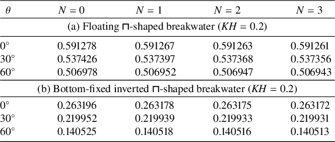
To examine the convergence of our models using the Galerkin approximation, we present the values of
 $|R|$
for varying numbers of terms (N) in the Galerkin approximation, as shown in Table 3. For this analysis, we select the parameters for floating
 $\boldsymbol {\sqcap }$
-shaped breakwater as
 ${w_1}/{H}$
= 0.5,
 ${w_2}/{H}$
= 1.0,
 ${h_1}/{H}$
= 0.65,
 ${h_2}/{H}$
= 0.45 and for bottom-fixed inverted
 $\boldsymbol {\sqcap }$
-shaped breakwater as
 ${w_1}/{H}$
= 0.5,
 ${w_2}/{H}$
= 1.0,
 ${h_1}/{H}$
= 0.35,
 ${h_2}/{H}$
= 0.55. Also, the porous effect parameter is taken as
 $G_1=G_2$
= 0.75 for both the breakwaters. It is evident from Table 3 that accuracy up to five figures (that is, an error estimate of
 $10^{-6}$
) has been achieved with
 $N=3$
(that is, four terms in the Galerkin approximation), demonstrating the accuracy of the present numerical scheme.
The reflection coefficients for (a) floating
 $\boldsymbol {\sqcap }$
-shaped and (b) bottom-fixed inverted
 $\boldsymbol {\sqcap }$
-shaped breakwater.

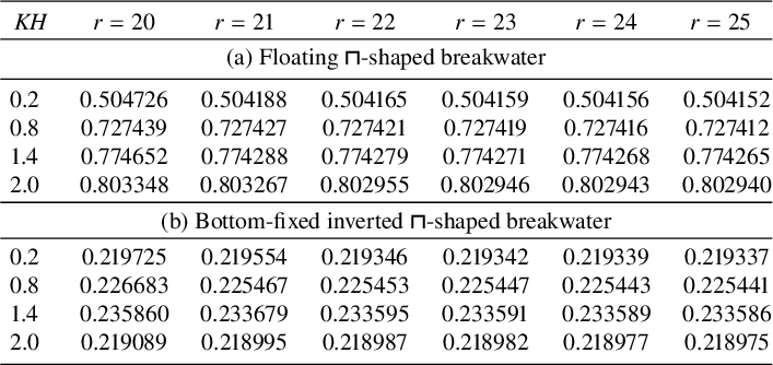
The convergence of the infinite series sum (arising in equation (3.6)) is verified in Table 4 by considering different truncation size r of that series. The parametric values are taken to be the same as in Table 3, with
 $\theta =75^\circ $
for both models, accordingly. Almost five-figure accuracy has been obtained by taking
 $r=25$
, which ensures the convergence of the infinite series. Therefore, four terms in the Galerkin approximation and
 $r=25$
in the truncated infinite series are considered for further parametric studies.
The reflection coefficients for (a) floating
 $\boldsymbol {\sqcap }$
-shaped and (b) bottom-fixed inverted
 $\boldsymbol {\sqcap }$
-shaped breakwater.

5 Verification of numerical models
To ensure the accuracy of two models, various well-known results are reproduced in this section. Hereafter, in all graphical depictions, we take the complex porous effect parameters of front and rear plates to be equal, that is, (
 $G_1$
=
 $G_2$
=G), unless otherwise stated.
For
 $\boldsymbol {\sqcap }$
-shaped floating breakwater.
-
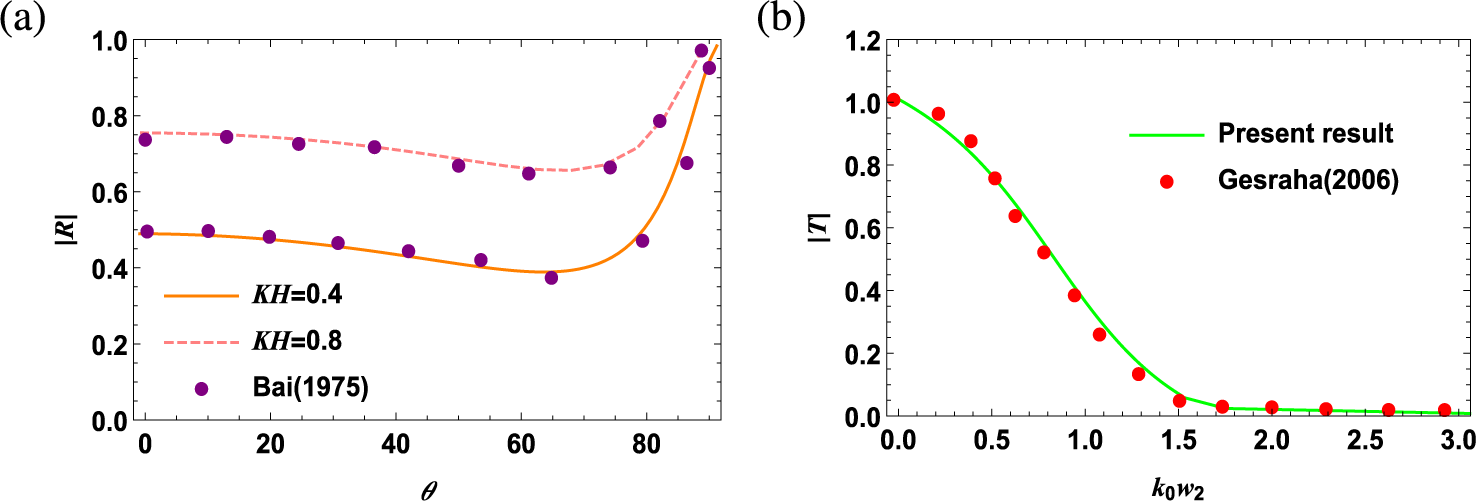
(i) The estimates of the reflection coefficient of the present model are compared with the graphical depiction by Bai [Reference Bai1, Figure 10] (rectangular floating structure). To do this, we first eliminate the porous side plate by taking
 ${h_1}/{H}={h_2}/{H}=0.5$
so that the
$\boldsymbol {\sqcap }$
-shaped floating model is transformed into a rectangular floating structure of draft
${d}/{H}=0.5$
. For such an approximation, the other parameters are taken as
${w_1}/{H}={w_2}/{H}=0.5$
and
$G=0$
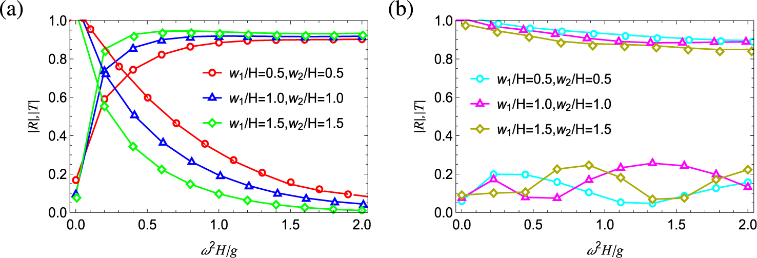
. As a result, Figure 2(a) follows fairly well the estimated curves described by Bai [Reference Bai1, Figure 10].
Figure 2
Verification of
$\boldsymbol {\sqcap }$
-shaped floating breakwater with existing results of the known literature. -
(ii) Another verification of the present numerical results for the transmission coefficient has been conducted by comparing them with the results of Gesraha [Reference Gesraha14] (
$\boldsymbol {\sqcap }$
-shaped floating breakwater with rigid thin plates). To do this, we neglect the porosity of thin plates by setting G=0, effectively converting them into rigid plates. As a result, the present structure is transformed into a
$\boldsymbol {\sqcap }$
-shaped floating breakwater with rigid thin plates. For such an approximation, we are taking
${h_1}/{H}={h_2}/{H}=0.3999, {d}/{H}=0.1176$
,
${w_1}/{H}={w_2}/{H}=0.3765$
and
$\theta =0^\circ $
. As observed in Figure 2(b), our estimates of
$|T|$
closely coincide with those of Gesraha [Reference Gesraha14, Figure 13].








For inverted
 $\boldsymbol {\sqcap }$
-shaped bottom-fixed breakwater.
-
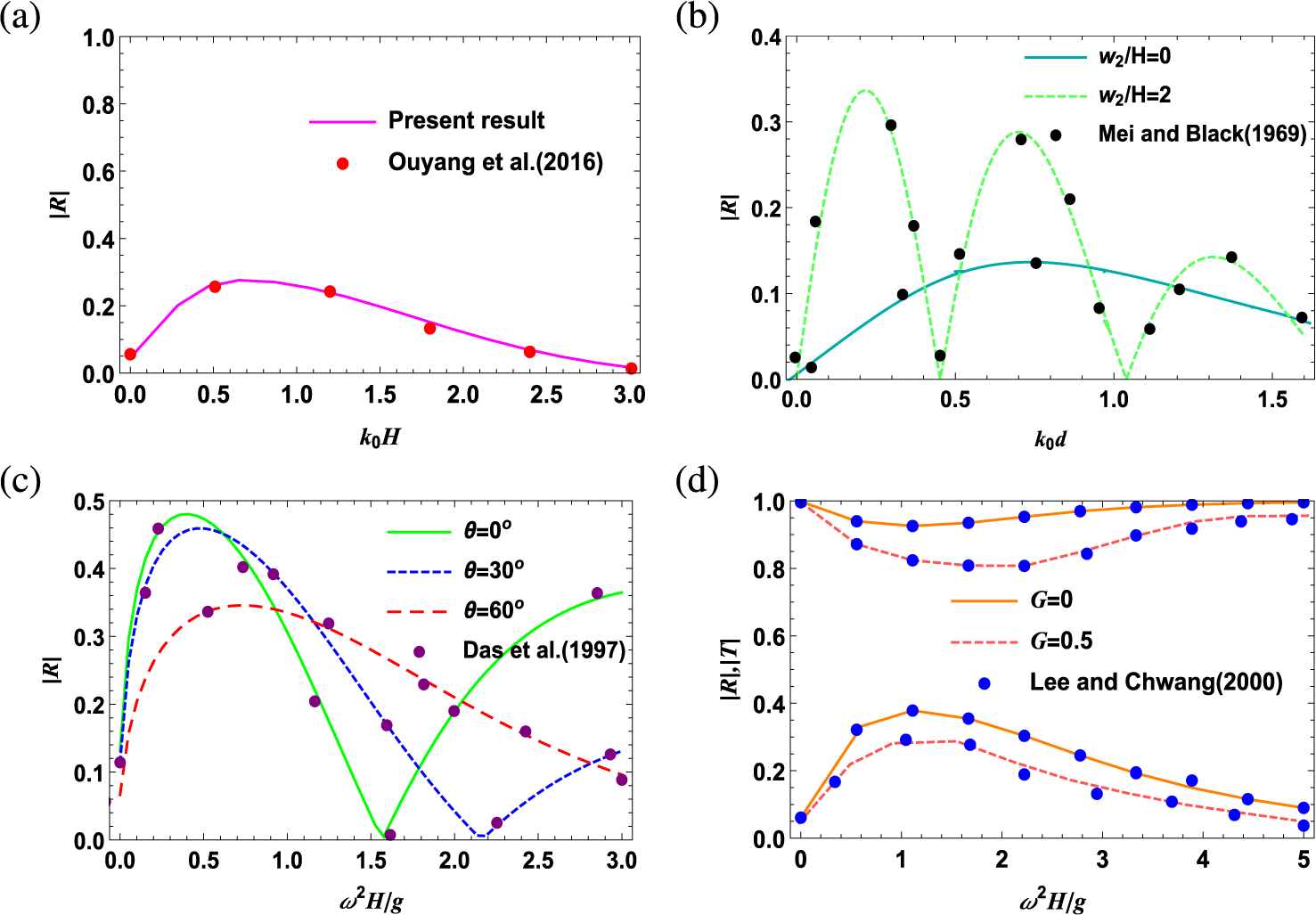
(i) To recover the result obtained by Ouyang et al. [Reference Ouyang, Chen and Tsai31, Figure 4(a)] (a rectangular bottom obstacle) for the case of normal incidence, we approximate the bottom-fixed inverted
$\boldsymbol {\sqcap }$
-shaped breakwater into a bottom obstacle of height
${d}/{H}=0.5$
. For such an approximation, we remove the porous plates by taking
${h_1}/{H}={h_2}/{H}=0.5$
and
$\textit {G}$
=0. The solid line shown in Figure 3(a) is plotted by taking the other parameters as
${w_1}/{H}={w_2}/{H}=0.25$
. Figure 3(a) depicts that the present data (solid line) coincide well with those of Ouyang et al. [Reference Ouyang, Chen and Tsai31] (represented by dots) and thereby establishes a very good agreement between our present results and the results of Ouyang et al. [Reference Ouyang, Chen and Tsai31].Figure 3Verification of inverted
$\boldsymbol {\sqcap }$
-shaped bottom-fixed breakwater with previously published literature. -
(ii) For the purpose of comparison with the numerical results of Mei and Black [Reference Mei and Black27, Figure 2] for the case of a submerged obstacle, we choose the parameters as
${h_1}/{H}={h_2}/{H}={d}/{H}=0.5$
,
${w_1}/{H}=0$
,
$\textit {G}$
=0 and
$\theta =0^\circ $
. So that the bottom fixed inverted
$\boldsymbol {\sqcap }$
-shaped breakwater transformed into a submerged obstacle as studied by Mei and Black [Reference Mei and Black27].Our computed results (represented by a solid line) are in excellent agreement with the results obtained by Mei and Black [Reference Mei and Black27] (represented by dots). The coincidence of Figure 3(b) gives another validation of the results determined from the present method.
-
(iii) Again, the present result of reflection coefficient is compared with the published results of Das et al. [Reference Das, Dolai and Mandal10]. We approximate a bottom-fixed inverted
$\boldsymbol {\sqcap }$
-shaped breakwater into a pair of thin rigid bottom-standing barriers by taking
${d}/{H}=0.999$
, so that the height of the rectangular structure is diminished. Also, we neglect the effect of porosity to convert the barriers into rigid by taking
$\textit {G}$
=0. The other parameters are taken as
${h_1}/{H}={h_2}/{H}=0.2$
,
${w_1}/{H}={w_2}/{H}=0.3$
. Figure 3(c) clearly indicates that our results almost coincide with those of Das et al. [Reference Das, Dolai and Mandal10, Figure 6]. -
(iv) Lastly, we verified our model with the results from Lee and Chwang [Reference Lee and Chwang22]. To compare the results of reflection and transmission coefficients with the analytical results obtained by Lee and Chwang [Reference Lee and Chwang22], for such an approximation, we choose
${h_1}/{H}=0.999, {h_2}/{H}=0.25, {d}/{H}=0.999$
, so that the bottom-fixed inverted
$\boldsymbol {\sqcap }$
-shaped structure is converted into the case of a bottom-standing porous barrier. The other parameters are taken as
${w_1}/{H}=0, {w_2}/{H}=0.001$
and
$\theta =0^\circ $
. The solid line in Figure 3(d) almost coincides with the result of Lee and Chwang [Reference Lee and Chwang22]. Thus, it is evident from Figure 3(d) that present results are in good agreement with the results of Lee and Chwang [Reference Lee and Chwang22].


















All the above-mentioned verifications clearly indicate that the present method is accurate for further numerical estimations.
6 Results and discussions
In this section, the two validated breakwater models are analysed to obtain various numerical estimates. For this purpose, a four-term Galerkin approximation is incorporated into the solution methodology. Furthermore, the system of equation (3.11) is solved by truncating the infinite series at r=25. The reasoning behind these considerations, along with the convergence analysis, has already been discussed in Section 4. To avoid lengthy terminology, we define the floating
 $\boldsymbol {\sqcap }$
-shaped breakwater and bottom-fixed inverted
 $\boldsymbol {\sqcap }$
-shaped breakwater as “Type-I” and “Type-II” breakwaters, respectively, throughout the whole section. As reflection and transmission coefficients play a key role in determining the behaviour of breakwaters, these coefficients are estimated for several values of the parameters. In addition to reflection and transmission coefficients, other physical quantities like the surface elevation, energy dissipation coefficient and horizontal drift force are also examined to assess their overall effectiveness.
6.1 Reflection and transmission coefficients
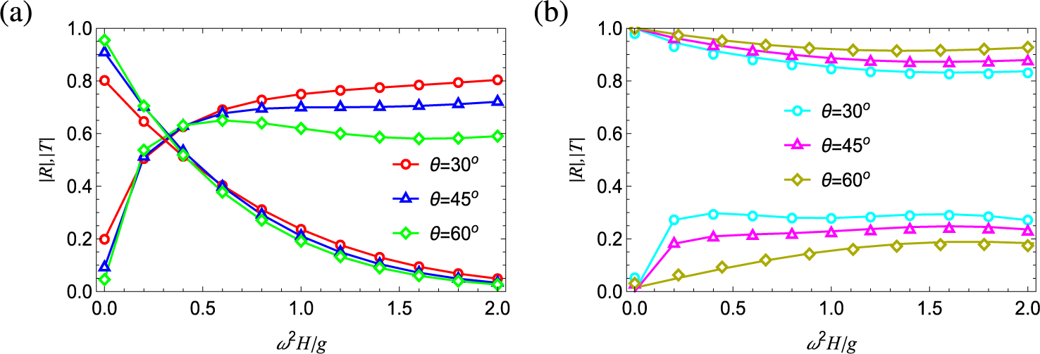
Figure 4 illustrates the impact of different incident angles on the reflection and transmission coefficients. For such an illustration, the parametric values of the Type-I structure are taken as
 ${h_1}/{H}$
= 0.65,
 ${h_2}/{H}$
= 0.45 and
 ${d}/{H}$
= 0.3, and for the Type-II structure as
 ${h_1}/{H}$
= 0.35,
 ${h_2}/{H}$
= 0.55 and
 ${d}/{H}$
= 0.7. The remaining parameters are taken as
 ${w_1}/{H}$
= 0.5,
 ${w_2}/{H}$
= 1.0 and
 $\textit {G}$
= 0.75 for both the breakwaters. From the two graphs, it is evident that as the angle of incidence increases, the reflection coefficient
 $|R|$
decreases for both types of breakwaters. The reduction in
 $|R|$
is more prominent in the case of the bottom-fixed structure for low frequency range (
 $\omega ^2H/g<$
0.5) as seen in Figure 4(b), whereas Figure 4(a) portrays that within such a frequency range, the variation is minimal for the floating structure. Beyond this frequency limit, an increase in the incident angle induces a more significant variation for Type I than for Type II. It is evident that the floating structure is clearly a more effective choice for reducing transmission, as anticipated.
Effect of varying angle of incidence on
 $|R|$
and
 $|T|$
for (a) Type-I and (b) Type-II breakwater.

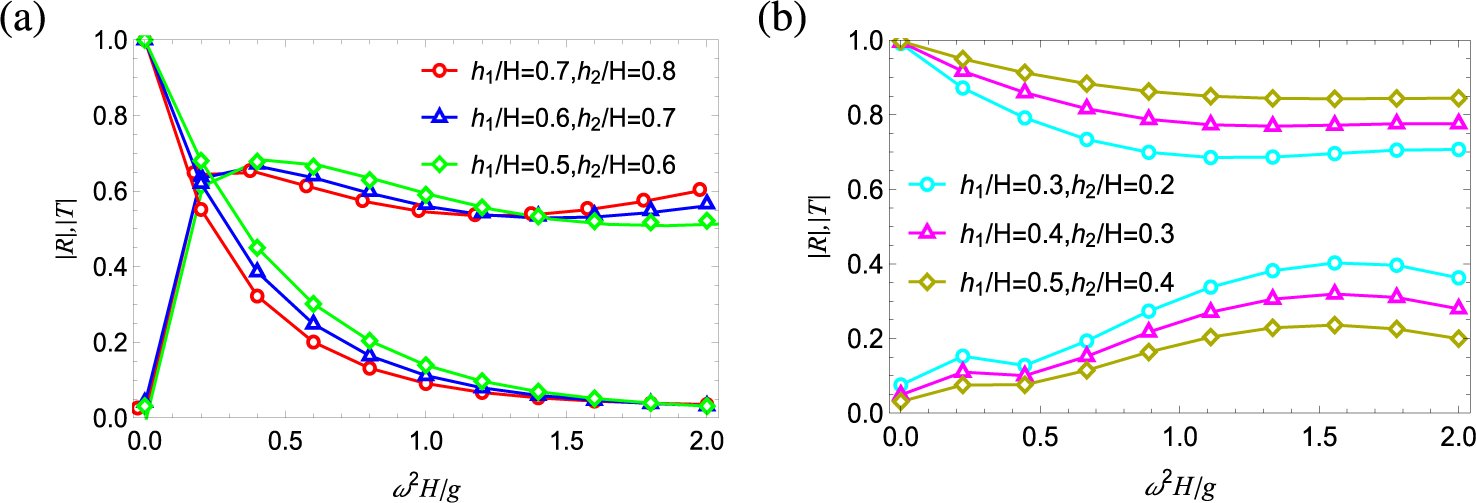
To assess the effectiveness of the two breakwaters, it is important to study the variation of one key quantity of interest; namely, the porous plate length. Therefore, Figure 5 represents the impact of variation of porous plate length on the reflection and transmission coefficients by taking
 ${w_1}/{H}$
= 1.25,
 ${w_2}/{H}$
= 0.75,
 $\theta =45^\circ $
and
 $\textit {G}$
= 1.0. Three graphs of
 $|R|$
and three graphs of
 $|T|$
are plotted in each of Figures 5(a) and 5(b) for the Type-I and Type-II structure, respectively, by taking three different values of
 ${h_1}/{H}$
and
 ${h_2}/{H}$
. For a certain angle of incidence and constant porosity, as the plate length increases,
 $|R|$
rises sharply; however, the variation is almost negligible for the Type-I structure, as observed in Figure 5(a) within a certain frequency range (
 $\omega ^2H/g<$
0.35). Beyond this, up to a certain range of
 $0.35<\omega ^2H/g<1.35$
, all the three graphs of
 $|R|$
decrease very slowly with an increase in plate length. The reverse trend in behaviour of
 $|R|$
is observed when
 $\omega ^2H/g> 1.35$
. However, the transmission coefficient decreases rapidly and approaches zero. This rapid decrease of
 $|T|$
with the increase of porous plate length may be due to the fact that the amount of wave energy dissipation through the pores increases with the increase of breakwater length. This will cause the waves to decay as they propagate through the plates. Figure 5(b) illustrates that a decrease in the plate length results in a reduction in the amplitude of reflection coefficient. Additionally, a notable variation in graphs of
 $|R|$
occurs in the higher frequency range as the plate length increases. It is observed from Figure 5 that
 $|R|$
remains consistently higher over a wide frequency range for the Type-I structure compared with Type II.
Effect of varying porous plate lengths on
 $|R|$
and
 $|T|$
for (a) Type-I and (b) Type-II breakwater.

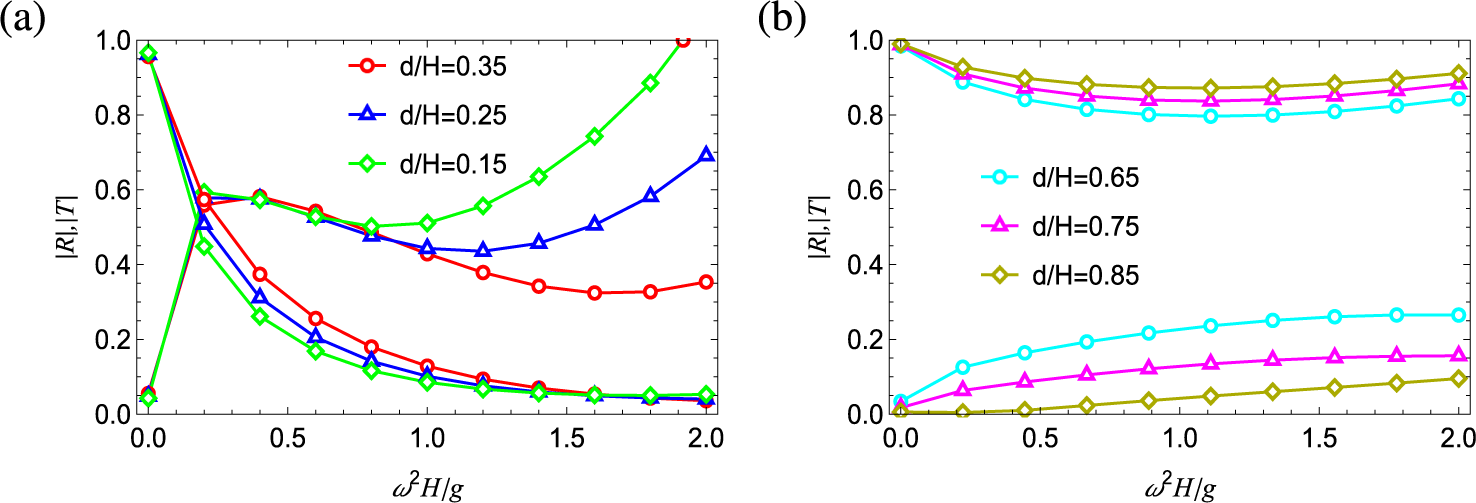
Sensitivity analysis is carried out in Figure 6 by varying the width of the breakwaters, that is, spacing between porous plates for fixed parameters
 $\theta =30^\circ $
and
 $\textit {G}$
= 0.5. The remaining parameters are taken for Type-I and Type-II structures as
 ${h_1}/{H}$
= 0.56,
 ${h_2}/{H}$
= 0.67 and
 ${d}/{H}$
= 0.34, and
 ${h_1}/{H}$
= 0.44,
 ${h_2}/{H}$
= 0.33 and
 ${d}/{H}$
= 0.66, respectively. Figure 6(a) demonstrates that wider structures can be more effective at achieving maximum reflection. In contrast, the transmission coefficient decreases rapidly as the breakwater width increases, as observed in Figure 6(a); however, in the high-frequency range, an increase in structural width results in a slower rate of decrease in wave transmission. This behaviour is observed when the energy dissipation due to the porous nature of the plates reaches its maximum capacity. This characteristic implies that, for practical applications such as shoreline protections, floating breakwater with wider plate spacing would be more advisable. However, as the spacing between porous plates increases, a more profound oscillatory pattern in
 $|R|$
is observed for the Type-II breakwater, although the amplitude of reflection remains very low as compared with Type I. Consequently, widening the rectangular structure has a minimal impact on reducing transmission for the bottom-fixed model compared with the floating one.
Effect of varying width on
 $|R|$
and
 $|T|$
for (a) Type-I and (b) Type-II breakwater.

The influence of the thick rectangular structure’s length on
 $|R|$
and
 $|T|$
is described in Figure 7. At lower wave frequencies,
 $|R|$
increases sharply, as shown in Figure 7(a); however, its variation with the length of the thick rectangular block is not significant. Eventually, it starts decreasing at intermediate frequencies (0.5
 $< \omega ^2H/g <$
1.0), indicating that the breakwater effectively dissipates or transmits wave energy. Figure 7(b) shows that as the length of the thick rectangular structure decreases,
 $|R|$
decreases monotonically. We consider
 $\theta =75^\circ $
,
 ${w_1}/{H}$
=
 ${w_2}/{H}$
= 0.6 and
 $\textit {G}$
= 1.25 +
 $\mathrm {i}$
, in plotting the graphs of Figure 7. The values of
 ${h_1}/{H}$
and
 ${h_2}/{H}$
are taken as 0.78, 0.56 in Figure 7(a) (Type I) and 0.22, 0.44 in Figure 7(b) (Type II).
Effect of varying length of the thick rectangular structure on
 $|R|$
and
 $|T|$
for (a) Type-I and (b) Type-II breakwater.

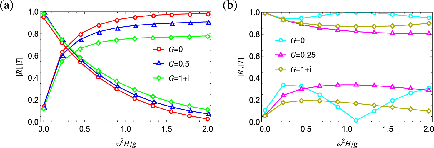
Figure 8 describes the effects of different porous-effect parameter (
 $\textit {G}$
) on reflection and transmission coefficients. The graphs of Figure 8 are depicted with
 $\theta =30^\circ $
,
 ${w_1}/{H}$
=
 ${w_2}/{H}$
= 0.5 and
 ${d}/{H}$
= 0.5. The remaining parametric values are taken as
 ${h_1}/{H}$
=
 ${h_2}/{H}$
= 0.65 for Type I and
 ${h_1}/{H}$
=
 ${h_2}/{H}$
= 0.35 for Type II. In both Figures 8(a) and 8(b), it is observed that as the porosity increases, the reflection coefficient decreases. Thus, as the plates become more transparent, more waves are able to pass through them, resulting in less reflection. Figure 8(a) exhibits that a decrease in porosity leads to greater restriction of water flow through plates at higher frequency, which in turn enhances the amount of reflection. A similar trend is seen for the bottom-fixed structure in Figure 8(b). However, at a particular frequency, when
 $\omega ^2H/g\simeq 1.1$
, the reflection coefficient drops to zero for rigid plates, indicating that there is no reflected wave at this point. This could be due to a resonance condition or the matching of impedance between the plate and water, leading to a perfect transmission and no reflection. Essentially, energy from the wave is entirely absorbed or transmitted by the plate, and no wave is reflected back into the seaside.
Effect of varying porosity of protruding plates on
 $|R|$
and
 $|T|$
for (a) Type-I and (b) Type-II breakwater.

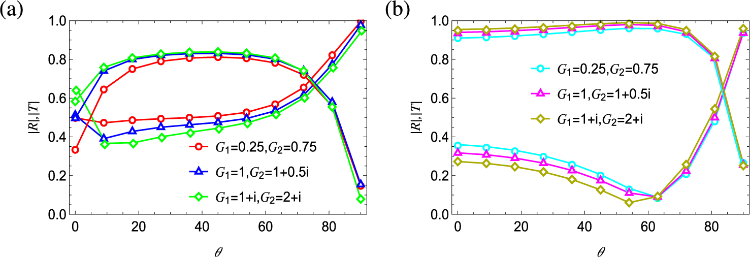
To illustrate the effect of different porous-effect parameters, reflection and transmission coefficients are plotted against incident angle for both breakwaters in Figure 9. To visualize how different values for each porous plate variation influences the wave scattering behaviour, we assume
 $G_1$
and
 $G_2$
are not equal. For such illustrations, we take
 ${w_1}/{H}$
=
 ${w_2}/{H}$
= 1.0 and
 $\omega ^2H/g$
= 0.2. The remaining parametric values are taken as
 ${h_1}/{H}$
= 0.55,
 ${h_2}/{H}$
= 0.65,
 ${d}/{H}$
= 0.35 for Type I and
 ${h_1}/{H}$
= 0.45
 ${h_2}/{H}$
= 0.35,
 ${d}/{H}$
= 0.65 for Type II. Three cases are considered: (i) when only the resistance effect is present on both porous plates (
 $G_1,G_2$
are both real); (ii) when only the resistance effect is present on the front plate, and both resistance and inertial effects are present on the rear plate (
 $G_1$
is real,
 $G_2$
is complex), and (iii) when both resistance and inertial effects are present on both plates (
 $G_1,G_2$
are both complex). If both the resistance and inertial effects are present on the porous plates, wave reflection is lower compared with the case where only the resistance effect is present, as shown in Figures 9(a) and 9(b). It is observed from Figure 9(a) that with an increase of incident angle, the reflection coefficient slightly decreases initially, then is followed by an increasing trend. Additionally, with an increase in the magnitude of porosity of the plates, the reflection coefficient decreases, whereas an increase in the incident angle initially leads to an increase in transmission, reaching a maximum value at an incident angle of
 $\theta \simeq 70^\circ $
. Beyond this angle, transmission begins to decrease and approaches towards zero. Further, Figure 9(b) shows that with an increase in the incident angle, the reflection coefficient initially decreases up to a certain angle of
 $\theta \simeq 60^\circ $
, after which it starts to increase. Moreover, as the magnitude of porosity decreases, the reflection coefficient increases, while transmission exhibits the opposite trend. For both cases, at higher incident angles, the reflection coefficient approaches unity as the porosity varies.
Effect of varying porosity of protruding plates on
 $|R|$
and
 $|T|$
against incident angle for (a) Type-I and (b) Type-II breakwater.

6.2 Free surface elevation
The free surface elevations are obtained from the following relation [Reference Karmakar and Guedes Soares17]:
 $$ \begin{align*} \eta(x)=\frac{i}{\sigma}\frac{\partial \phi}{\partial y}\quad\mbox{on~}y=0. \end{align*} $$
For graphical representation, we symbolize
 $\eta (x)$
as
 $$ \begin{align*} \eta \equiv \eta(x)\mbox{~when~} \begin{cases} x<-1&\mbox{for incident region,}\\ -1<x<2&\mbox{for inside breakwater region,}\\ x>2 &\mbox{for transmitted region.} \end{cases} \end{align*} $$
The free surface elevation
 $\eta $
is plotted against distance x for various values of incident angle and porous-effect parameter, as shown in Figures 10 and 11, respectively. From Figure 10, it is observed that the free surface elevation in the transmitted region decreases with the increase in angle of incidence. Additionally, free surface elevation in the transmitted region is observed to be much less as compared with the incident region for both models. The reduction in
 $\eta $
is however very high due to the presence of the Type-I structure compared with the Type-II structure indicating that floating breakwater attenuates the wave height in the transmitted region more significantly than a bottom-fixed breakwater. However, variation of the porous effect parameter on surface elevation shows a similar behaviour for both types of breakwaters. As the porosity increases,
 $\eta $
decreases in the incident region, although a contrasting behaviour is depicted in the transmitted region, as observed in Figure 11. Moreover, it is noticed that the amplitude of
 $\eta $
is consistently higher in both incident and transmitted regions for the Type-I structure compared with the Type-II structure. Further, the wavelength remains constant and unaffected by porosity for both types of breakwaters in both the regions.
Effect of varying incident angle on
 $\eta $
for (a) Type-I and (b) Type-II breakwater.

Effect of varying porosity of protruding plates on
 $\eta $
for (a) Type-I and (b) Type-II breakwater.

6.3 Energy dissipation coefficient
When a wave interacts with a porous plate breakwater, the total wave energy is distributed into three components. The first component is the reflected wave energy, the second is dissipated wave energy and the third is transmitted wave energy that passes through the breakwater. According to the law of energy conservation, the total energy balance can be expressed by the following equation, as derived by Burcharth and Hughes [Reference Burcharth and Hughes5]:
 $$ \begin{align*} E_i = E_r + E_t + E_d. \end{align*} $$
Here,
 $E_i$
,
 $E_r$
,
 $E_t$
and
 $E_d$
are the energy of the incident wave, reflected wave, transmitted wave and dissipated wave, respectively. Following this energy balance formula, the energy dissipation coefficient can be written as follows:
 $$ \begin{align*} D_E= 1-|R|^2-|T|^2. \end{align*} $$
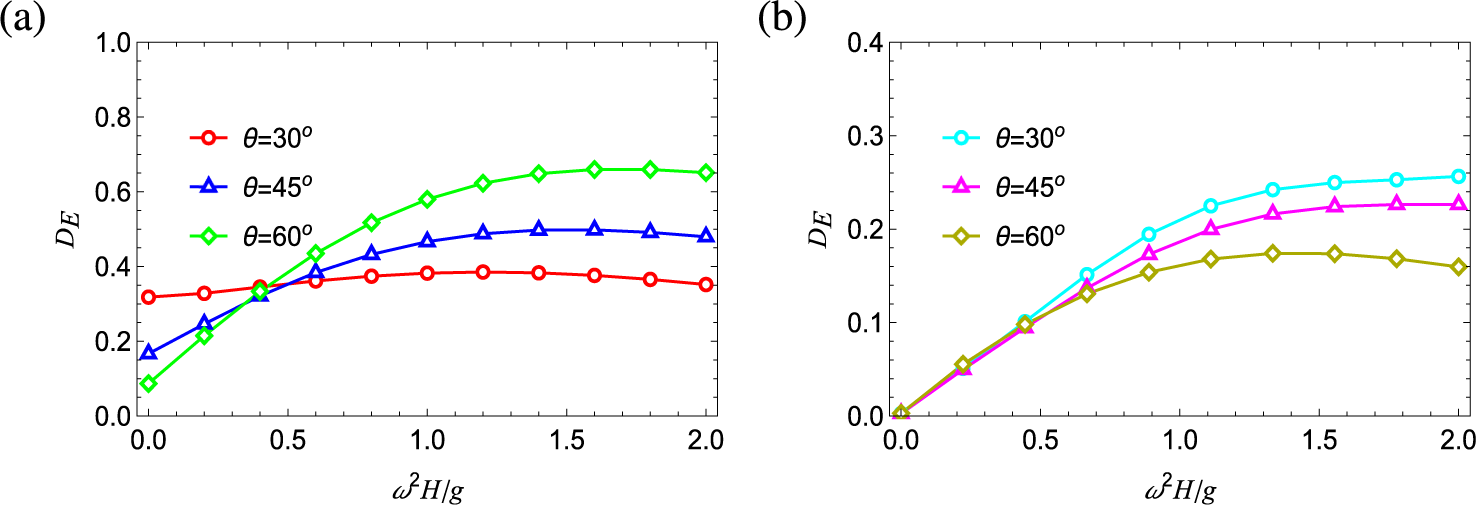
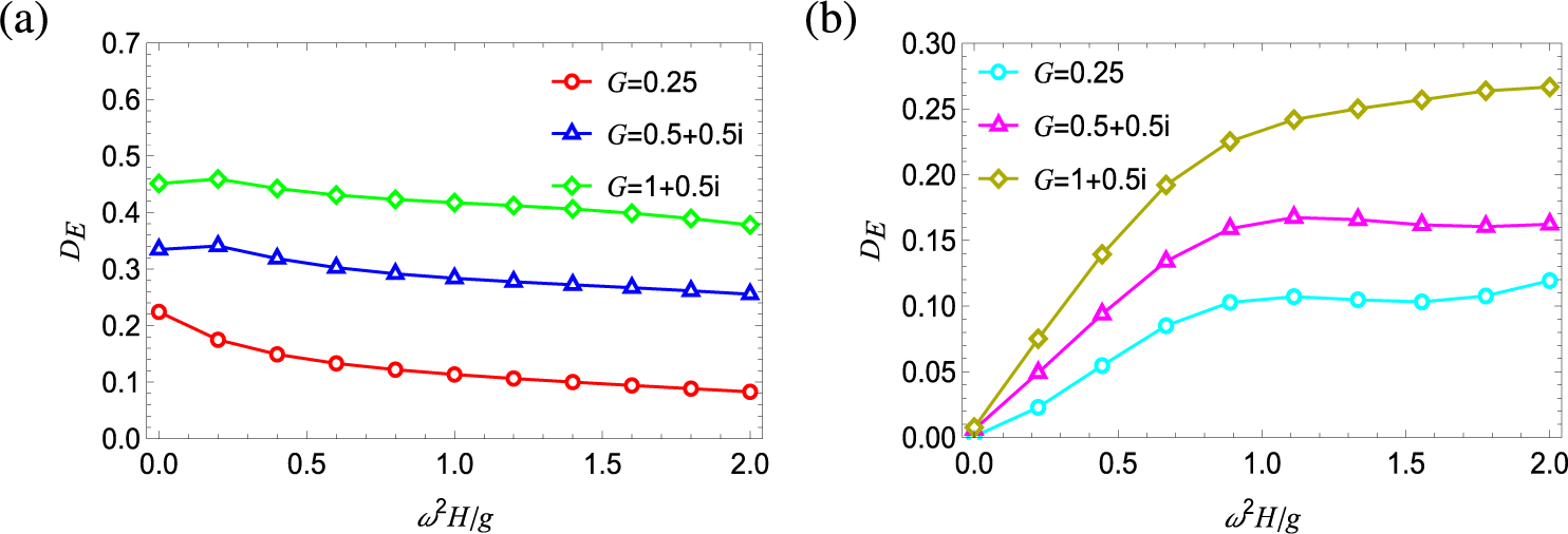
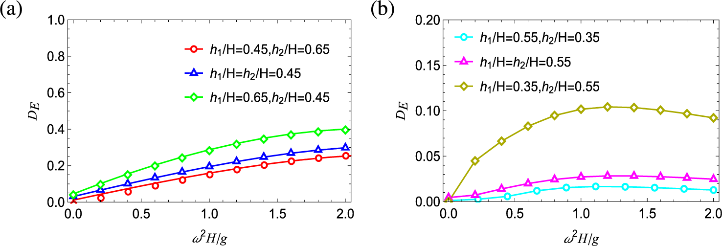
Figures 12–14 present the variation of energy dissipation coefficient due to the variation in plate length, incident angle and porosity of plates. As shown in Figure 12(a), energy dissipation decreases with an increase in the angle of incidence for Type-I breakwaters up to a certain frequency
 $\omega ^2H/g\simeq 0.4$
. After this point, dissipation increases as the angle of incidence increases. Figure 14(b) however suggests that the dissipation reduces for Type-II breakwater with increase in the angle of incidence. Figure 13 depicts the energy dissipation for various values of porous effect parameters. For both types of breakwaters, energy loss increases as the plate porosity increases. Over a wide frequency range, the bottom-fixed structure experiences a higher energy loss, which gradually increases with increase in porous effect parameter. However, for the floating structure, the energy loss slightly decreases. Comparing the two models, it is clear that energy dissipation is higher for the Type-I structure compared with the Type-II structure. To explore the influence of length of the porous plate on energy dissipation, we examine three different cases to highlight the conditions under which energy loss is most significant (Figure 14). Both graphs clearly depict that energy dissipation is higher when the front porous plate is longer than the rear plate. This is likely because a longer front plate exposes a larger surface area to the incoming wave, allowing for greater energy absorption and dissipation.
Effect of incident angle on
 $D_E$
for (a) Type-I and (b) Type-II breakwater.

Effect of plate porosity on
 $D_E$
for (a) Type-I and (b) Type-II breakwater.

Effect of porous plate length on
 $D_E$
for (a) Type-I and (b) Type-II breakwater.

6.4 Horizontal drift force
Following Longuet and Higgins [Reference Longuet-Higgins23], the dimensionless horizontal drift force on both breakwater models is defined as
 $$ \begin{align*} F_D=\frac{A H}{8(w_2+w_1)}\bigg(1+\frac{2kH}{\sinh 2kH}\bigg)(1+|R|^2-|T|^2), \end{align*} $$
where A is the incident wave amplitude.
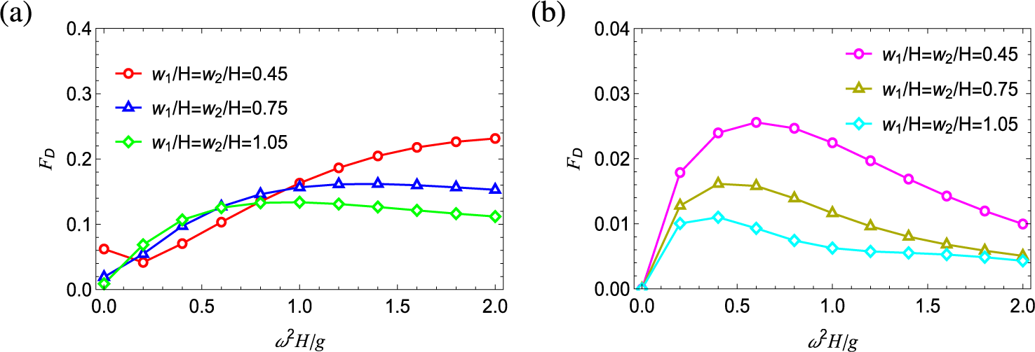
Figure 15 depicts the relation between horizontal drift force and wavenumber by varying the width of breakwaters taking
 $\theta =45^\circ $
,
 $\textit {G}$
=
 $0.25+0.5{i}$
and
 ${d}/{H}$
= 0.55, and the values of
 ${h_1}/{H}$
and
 ${h_2}/{H}$
are taken as 0.76, 0.66 for Type I and 0.24, 0.34 for Type II. For Type-I breakwater, as the width increases, the magnitude of drift force decreases in the higher frequency range as observed in Figure 15(a). This is likely because a thicker breakwater attributes better dissipation in wave energy, causing less energy to be transferred into horizontal motion at higher frequencies. Additionally, for a very wide structure, the drift force reaches a constant value, indicating that the breakwater’s width effectively stabilizes the horizontal drift force, especially for higher frequencies. For a Type-II structure, a narrower breakwater tends to produce a higher peak in drift force at lower frequencies. This suggests that narrower breakwaters are more efficient at transferring wave energy into horizontal motion for lower-frequency waves. After reaching the peak, the drift force starts to decrease at higher frequencies, likely due to the increased dissipation of wave energy by the wider breakwater.
Effect of width of breakwater on
 $F_d$
for (a) Type-I and (b) Type-II breakwater.

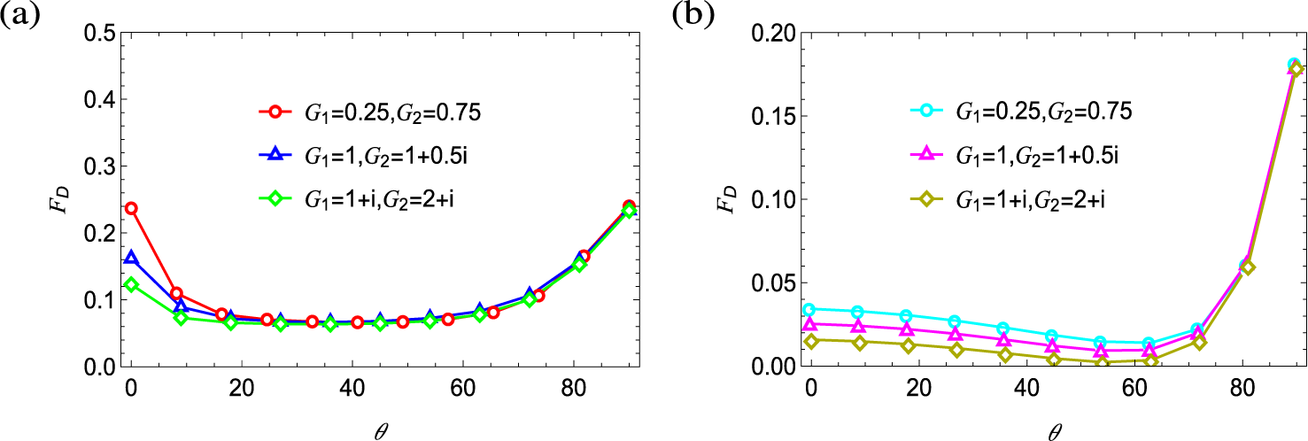
The influences of varying porosity of protruding plates on
 $F_D$
against incident angle are plotted in Figure 16 for both breakwaters. For such illustrations, we choose
 ${G_1\neq G_2}$
,
 ${w_1}/{H}= {w_2}/{H}=1.0$
and
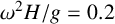 ${\omega ^2H}/{g}=0.2$
. The other remaining parametric values are taken as
 ${h_1}/{H}$
= 0.55,
 ${h_2}{H}$
= 0.65,
 ${d}/{H}$
= 0.35 for Type I and
 ${h_1}/{H}$
= 0.45
 ${h_2}/{H}$
= 0.35,
 ${d}/{H}$
= 0.65 for Type II. In this analysis, we examine the same cases as those presented in Figure 9. As a result, Figure 16 shows that when both inertial and resistance effects are present on both plates, the drift force is lower compared with the case where only the resistance effect is considered for both types of breakwaters.
Effect of varying porosity of protruding plates on
 $F_D$
against incident angle for (a) Type-I and (b) Type-II breakwater.

7 Conclusions
This study develops a semi-analytical approach to examine the wave interactions with two breakwater designs: (a) a floating
 $\boldsymbol {\sqcap }$
-shaped breakwater and (b) a bottom-fixed inverted
 $\boldsymbol {\sqcap }$
-shaped breakwater with porous side plates, both in finite-depth water. The mathematical formulation employs a matched eigenfunction method in reducing the problem to a set of coupled integral equation of first kind. These integral equations are then solved by the Galerkin approximation method with suitable basis functions. We have validated our present method by approximating the results with existing results and provided new numerical findings. Numerical estimates of physical quantities, such as
 $|R|$
,
 $|T|$
,
 $\eta $
,
 $D_E$
and
 $F_D$
, are presented through graphical representations for various configurations of breakwaters. The key conclusions are summarized here.
-
• Graphs of scattering coefficients plotted for various incident angles reveal that floating
$\boldsymbol {\sqcap }$
-shaped structure is more effective than an inverted bottom-fixed one in terms of wave transmission reduction for the high-frequency regime. With the increase in incident angle, less energy is transmitted through the structure, leading to higher dissipation of wave energy. Furthermore, as the incident angle becomes more oblique, the free surface elevation in the transmitted wave region decreases more significantly for Type I than for Type II. -
• Increasing the porous plate length significantly impacts
$|R|$
for longer wavelengths, while causing a rapid decrease in
$|T|$
. This is due to longer porous plates enhancing wave energy dissipation. Interestingly, when the front plate exceeds the size of rear plate, energy dissipation increases noticeably for both structures. Therefore, incorporating longer porous plates in the design of these breakwaters can be more beneficial. -
• Widening the Type-I breakwater enhances wave energy reflection and reduces the force exerted on the structure, improving its overall stability. Furthermore, a thicker breakwater is observed to be more effective in achieving complete reflection for Type I. Conversely, narrowing the Type-II breakwater diminishes the oscillatory pattern of the reflection coefficient and significantly reduces the drift force, making the structure more efficient at dissipating wave energy and minimizing wave-induced loads.
-
• The rate of change in the transmission coefficient is larger for variation of porous plate length than for variation of width of breakwater. Therefore, increasing the length of the porous plate can attenuate incident wave faster than width.
-
• Increasing the porosity of plates enhances wave transmission at high frequencies for both types of breakwaters. As the breakwaters become more transparent, the free surface elevation decreases in the transmitted region, but increases in the incident region. In both regions, the wavelength of
$\eta $
remains unchanged despite variations in porosity. Therefore, porosity should be selected judiciously to optimize performance, benefiting the cost-effective design of breakwaters. -
• Energy dissipation analysis indicates that
$D_E$
is highly sensitive to plate porosity for both models, with the magnitude being higher for Type-I than Type-II breakwater. -
• When both inertial and resistance effects are present on both plates, the reflection coefficient and drift force are lower than the case where only the resistance effect is considered for both types of breakwaters.


This study provides valuable insights of the breakwater performance, highlighting the potential for further exploration of hydrodynamic parameters. However, long-term field studies are needed to evaluate their broader impact on coastal processes. The present wave propagation problem can be extended further for multiple
 $\boldsymbol {\sqcap }$
-shaped breakwaters in deep or finite depth water by employing a similar methodology as used in the present paper.
Acknowledgments
The authors would like to gratefully acknowledge the Editor and Reviewers for their valuable comments and suggestions to improve the quality of the manuscript. This work is partially supported by Science and Engineering Research Board, Department of Science and Technology, India [grant number TAR/2022/000107].