
I. INTRODUCTION
Annealing twin boundaries (TBs) are common in face-centered cubic materials with medium and low stacking fault energies,Reference Carpenter and Tamura1,Reference Mahajan, Pande, Imam and Rath2 such as 316L stainless steel. TBs have an extraordinary morphology that is generally a straight line in a two-dimensional (2D) observation, arousing a strong research interest since early in the last century.Reference Carpenter and Tamura1 Compared with random boundaries, TBs have not only a conspicuous morphology but also special properties, such as lower boundary energy and increased resistance to impurity segregation, precipitation of minority phases,Reference Li, Xia, Zhou, Chen and Hu3 and intergranular degradation.Reference Lin, Palumbo, Erb and Aust4–Reference Engelberg, Marrow, Newman, Babouta, Shipilov, Jones, Olive and Rebak11 The concept of “grain boundary design and control,” proposed by Watanabe,Reference Watanabe12 aimed to improve grain boundary (GB)-related properties of materials via increasing the proportion of so-called special boundaries such as TBs. This research field is now well known as “grain boundary engineering”,Reference Michiuchi, Kokawa, Wang, Sato and Sakai5,Reference Liu, Xia, Li, Zhou, Bai, Su and Cai13–Reference Barr, Leff, Demott, Doherty and Taheri27 which has been successfully applied in many materials, such as stainless steels,Reference Michiuchi, Kokawa, Wang, Sato and Sakai5,Reference Hu, Xi, Li, Liu, Zhou, Chen and Wang7,Reference Engelberg, Newman and Marrow21 Ni-based alloys,Reference Liu, Xia, Li, Zhou, Bai, Su and Cai13,Reference Liu, Xia, Li, Zhou and Bai14 and Cu-based alloysReference Randle16 through thermomechanical processing.
The misorientation component of the GB character is generally described using the coincidence site lattice (CSL) model. In the CSL model, the ∑-value is the reciprocal density of coincident lattice sites of the two grains adjacent to the boundary, and boundaries with low-∑ values (∑-value ≤ 29) are generally considered special. The proportion of low-∑ CSL boundaries can be increased from 40% to more than 75% by GB engineering.Reference Michiuchi, Kokawa, Wang, Sato and Sakai5,Reference Liu, Xia, Li, Zhou, Bai, Su and Cai13–Reference Katnagallu, Mandal, Nagaraja, De Boer and Vadlamani22 Of the new special boundaries, about 80% are TBs, which are designated as ∑3 in the CSL model. However, until recently, all the related results were derived from microstructure data in 2D maps. The low-∑ CSL boundary proportions were calculated using the length or the number of boundaries observed on 2D sectional maps rather than the actual boundary area or total number of boundaries in 3D microstructures.
Besides the GB character distribution, other microstructural characteristics should be considered to evaluate the effectiveness of GB engineering, such as the size of twin-related domains and GB connectivity. A twin-related domainReference Liu, Xia, Li, Zhou, Bai, Su and Cai13,Reference Liu, Xia, Li, Zhou and Bai14,Reference Xia, Zhou and Chen19,Reference Gertsman and Henager23–Reference Barr, Leff, Demott, Doherty and Taheri27 is a crystallographically constrained domain in which all grains can be connected via only ∑3n boundaries. A recent study has compared the twin-related microstructures in a conventional and a GB-engineered copper in 3D, finding that twin-related domains are much larger in the GB-engineered copper.Reference Lind, Li and Kumar26 The improvement of the resistance to intergranular degradation by GB engineering is substantially related to the random boundary connectivity.Reference Michiuchi, Kokawa, Wang, Sato and Sakai5,Reference Kobayashi, Kobayashi and Watanabe17,Reference Kumar, King and Schwartz28–Reference Tokita, Kokawa, Sato and Fujii31 However, until recently, 3D studies of GB networks were rare, except for computer simulation. Simulations showed that while the fraction of special boundaries that is required to break up a 2D network of random boundaries is 0.35, special boundary fractions of 0.775–0.85 are required to disrupt the connectivity of random boundaries in 3D.Reference Frary and Schuh32 A latest paper from our groupReference Liu, Xia, Zhou, Bai and Rohrer33 investigated the characteristics of the 3D GB network of 316L stainless steel before and after GB engineering. The same raw data were used in the current paper, but the current study focuses on the 3D TBs. The twin-related domains in the GB-engineered 316L are larger and have more complex topological structures than that in the conventional 316L.Reference Liu, Xia, Zhou, Bai and Rohrer33 However, the TB fraction in triple junctions and quadruple junctions only has a slight increase after GB engineering.
Our current understanding of TBs is based mostly on observations from 2D sections. Based on 2D observations, the morphologies of twins have been classified into four categories: grain-corner twins, complete parallel-sided twins that span a grain, incomplete parallel-sided twins that do not span the grain, and island twins.Reference Mahajan, Pande, Imam and Rath2,Reference Meyers and Murr34 An early 3D study by BystrzyckiReference Bystrzycki and Przetakiewicz35 showed that there were only two types of twins: lamellar twins and corner twins. However, because of the low resolution of the 3D microstructure in Ref. Reference Bystrzycki and Przetakiewicz35, it is uncertain whether other types of twins exist or not. In addition, because some morphologically complex TBs can be observed in 2D-EBSD (electron backscatter diffraction) maps of GB-engineered materials,Reference Liu, Xia, Li, Zhou, Bai, Su and Cai13–Reference Randle and Coleman15,Reference Kobayashi, Kobayashi and Watanabe17,Reference Wang, Dallemagne, Hou and Yang18,Reference Telang, Gill, Kumar, Teysseyre, Qian, Mannava and Vasudevan36 the actual morphologies of these boundaries are unclear. Further 3D characterization of GB-engineered microstructures is necessary to quantify the differences between conventional and GB-engineered materials.
The 3D microstructure of a 316L stainless steel was measured before and after GB engineering by 3D-EBSD to determine the changes brought about by GB engineering. Although most 3D-EBSD data have been collected using focused ion beam (FIB) serial sectioning combined with EBSD mapping,Reference Kelly, Glowinski, Nuhfer and Rohrer37–Reference Uchic, Groeber, Dimiduk and Simmons39 the field of view that can be sectioned by FIB is rated small, usually less than 100 μm. This means that in alloys with grain sizes in the range of 30–40 μm, very few grains are contained in the field of view. Therefore, in the current work, 3D-EBSD data have been collected by coupling EBSD mapping with serial sectioning by mechanical polishing.Reference Lewis, Bingert, Rowenhorst, Gupta, Geltmacher and Spanos40–Reference Spowart43 This makes it possible to map fields of view as large as 800 μm, containing hundreds of grains in microstructures with an average grain diameter in the range of 30–40 μm. A paper, focused on the 3D characteristics of the GB network before and after GB engineering using the 3D-EBSD data, had been published elsewhere.Reference Liu, Xia, Zhou, Bai and Rohrer33 In the current paper, the morphology, area fraction, number fraction, and connectivity of TBs in 3D before and after GB engineering have been measured. The results show some characteristics of GB-engineered microstructures that cannot be observed in 2D maps and reveal that the key point with respect to GB engineering process is the increased TB number fraction rather than area/length fraction to disrupt the connectivity of random boundary network.
II. EXPERIMENTAL
A commercially available hot-forged 316L stainless steel with a thickness of 40 mm, which has a chemical composition (wt%) of Cr 16.26, Ni 10.10, Mo 2.08, C 0.028, Si 0.47, Mn 1.03, P 0.044, S 0.005, and Fe in balance, was used in this work. A block with a size of 40 × 50 × 134 mm3 was machined using a wire-cut electrical discharge machine from the as-received 316L plate. Subsequently, it was hot-rolled to a 50% reduction in thickness at 1000 °C followed immediately by water quenching. The sample was then cut into three pieces. One piece (316LL) was annealed at 1050 °C for 150 min and water quenched. The second piece (316LS) was annealed at 1000 °C for 30 min and water quenched. These processes created uniformly recrystallized microstructures with different grain sizes. The third piece (316LGBE) of the material was thermomechanically processed to increase the fraction of low-∑ CSL boundaries, and the process referred to as GB engineering. It was first annealed at 1000 °C for 30 min and water quenched. Next, it was warm-rolled with one pass to a 5% thickness reduction at a starting temperature of 400 °C and then water quenched. Finally, it was annealed at 1100 °C for 60 min and water quenched for full recrystallization.
The three samples were investigated by 3D orientation imaging microscopy. Mechanical polishing was used to create a series of parallel 2D sections. A CamScan Apollo 300 field emission scanning electron microscope (CamScan, Cambridge, United Kingdom) equipped with an Oxford/HKL EBSD system (Oxford Instruments, Oxford, United Kingdom) was used to measure crystal orientation data on the cross section after each polishing step. The workflow for the 3D-EBSD data acquisition could be described as follows: mechanical polishing → thickness reduction measurement → marking the regions of interest by using microhardness indents → EBSD mapping. Highly precise serial sectioning is a key step during the 3D-EBSD collection, but the norm of precision is related to the grain size of the measured material. A section thickness less than one 10th of the average grain diameter is an appropriate precision. 2D EBSD maps of the three samples, 316LL, 316LS, and 316LGBE, showed that their average grain diameters are 50 μm, 33 μm, and 47 μm, respectively. Therefore, during 3D-EBSD data acquisition, the target values for thickness reduction in each polishing cycle were set as 2.5 μm, 2.5 μm, and 5 μm for 316LL, 316LS, and 316LGBE, respectively. The samples were polished under a fixed load and the time was varied to achieve the targeted material removal. Additionally, a Buehler polishing cloth with a polishing suspension of sol–gel produced alumina (0.05 μm) was used to make sure that the surface after each polishing cycle was sufficiently crystalline to produce diffraction patterns suitable for EBSD mapping. Finally, a total of 101 sections were collected with an average section thickness of 2.65 and 2.55 μm for samples 316LL and 316LS, respectively, and a total of 70 sections were collected with an average section thickness of 5.39 μm for sample 316LGBE. The field of view for the EBSD maps on each section is 600 × 600 μm with a step size of 2.5 μm for samples 316LL and 316LS, and it is 800 × 800 μm with a step size of 5 μm for sample 316LGBE.
Extensive post-processing is required to interpret 3D-EBSD data. In this work, open source software was used for the reconstruction and quantitative analysis of the microstructures. The 2D EBSD orientation maps were reconstructed into 3D microstructures using Dream.3D v4.2.5004.Reference Groeber and Jackson44 ParaView v4.3.1Reference Ayachit45 was used to visualize the 3D microstructure. Dream.3D was used to obtain some quantitative results, such as grain size, grain orientation, and the number of nearest neighbors for each grain.Reference Groeber and Jackson44,Reference Groeber, Ghosh, Uchic and Dimiduk46–Reference Bhandari, Sarkar, Groeber, Uchic, Dimiduk and Ghosh48 Dream.3D was also used to identify the TBs according to the Brandon criterion.Reference Brandon49 In addition, some in-house developed Matlab programs were used to measure the sizes of 3D grain boundaries and to identify the connectivity of random boundaries or TBs, noting here that all high angle boundaries except for ∑3 were identified as random boundaries.
III. RESULTS
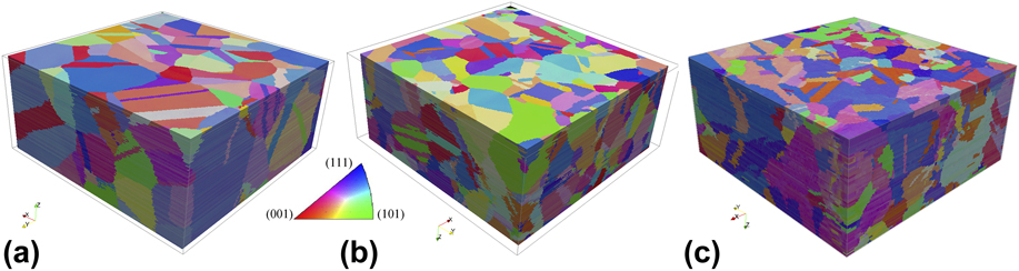
The reconstructed 3D-EBSD microstructures of samples 316LL, 316LS, and 316LGBE are shown in Fig. 1, containing 440 (2102), 1540 (8624), and 1543 (7053) grains (grain boundaries), respectively, and the grains are distinguished by using colors correlated with their orientations. The average 3D grain diameters (equivalent spherical diameters) are 41.4 μm (316LL), 30.0 μm (316LS), and 38.3 μm (316LGBE), where the border intersecting grains were taken into account because many large grains were intersected by the borders. This work will focus on comparing the TBs and GB networks in the GB-engineered 316L with those in the conventional 316L.
Visualizations of the three 3D-EBSD microstructures: (a) 316LL (600 × 600 × 267.6 μm3), (b) 316LS (600 × 600 × 257.5 μm3), and (c) 316LGBE (800 × 800 × 377.3 μm3). The grains were colored by using the IPF-Z code.

A. TB classification
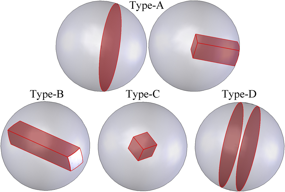
On the basis of the current results, 3D TBs can be classified into four categories according to their 3D morphologies: single-face TBs (type-A), tunnel TBs (type-B), occluded TBs (type-C), and parallel-multiplanar TBs (type-D), as shown in Fig. 2. The topological terminology “Boundary”Reference Armstrong50 was used to classify TB shape. In this context, the term boundary refers to the number of “boundary circles” in the homeomorphic sphere of a TB. These “boundary circles” are also referred to as “holes” and we shall use that latter term to avoid confusion with grain boundaries. The type-C TB is homeomorphic to a sphere so the occluded (type-C) TB has zero holes. In the same way, the type-A TB is homeomorphic to a sphere with one hole and the type-B TB has two or more holes. The type-D TB is an assembly of two or more parallel type-A TBs.
Schematic showing the TB classification according to the 3D morphologies: (type-A) single-face TB, (type-B) tunnel TB, (type-C) occluded TB and (type-D) parallel-multiplanar TBs.

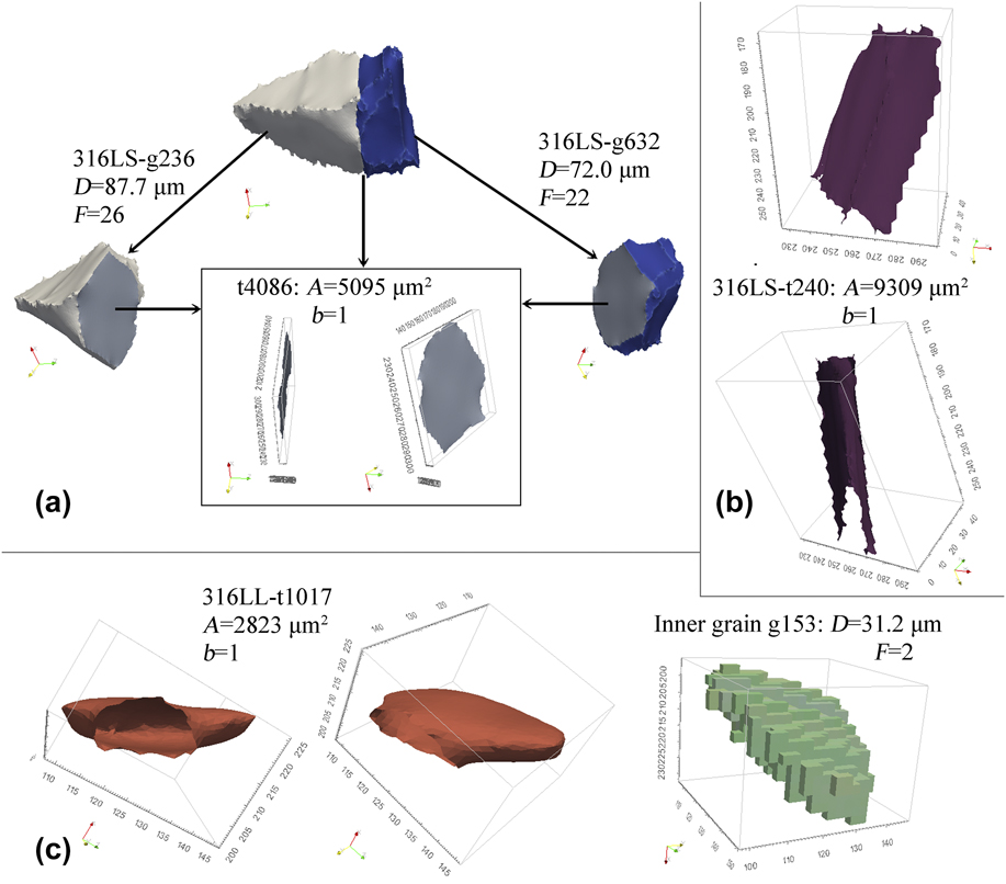
Three typical examples of type-A TBs are shown in Fig. 3. The TB in Fig. 3(a) is an approximate plane from specimen 316LS, and the two grains forming the TB are shown in Fig. 3(a) as well. In 2D maps, the observed morphology of the TB should be a straight line, which corresponds to a grain-corner twin in a 2D study.Reference Mahajan, Pande, Imam and Rath2,Reference Meyers and Murr34 In Fig. 3(b), the TB t240 from 316LS has the shape of a folded plane, but the observed morphology of this TB in 2D maps may be a grain-corner twin or a completely parallel-sided twin or an incompletely parallel-sided twin, depending on the cross section. Figure 3(c) shows a sack-shaped TB, in which a grain was semiclosed, and its observed morphology in 2D maps may be an occluded twin or an incomplete parallel-sided twin. Although the three TBs in Fig. 3 have different shapes, all of them have one hole so they are classified as type-A.
Examples of single-face TBs (type-A): (a) planar TB t4086 which is the interface of grains g236 and g632 from sample 316LS; (b) folded planar TB; (c) a sack-shaped TB and its inner raw grain (without surface smoothing), where “316LS-g236” indicates that the grain has an ID g236 in sample 316LS; “t4086” is a TB ID; ‘D’ means the diameter of equivalent sphere of the grain; ‘F’ means the number of GBs of the grain; ‘A’ means the GB area; ‘b’ means the number of “boundaries” in the homeomorphic surface of the TB-based on topology.

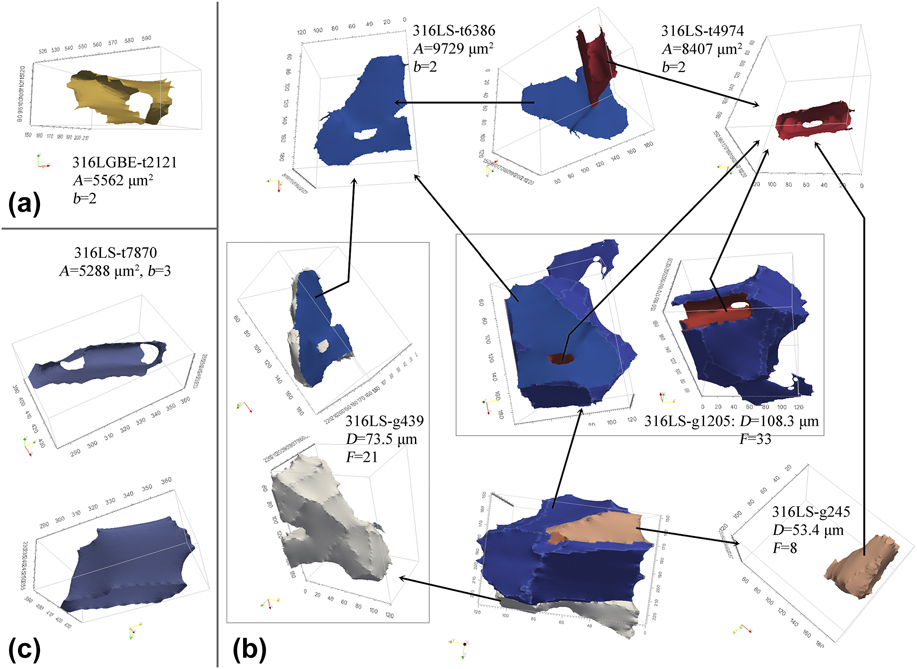
Four typical TBs of type-B are shown in Fig. 4. The TB in Fig. 4(a) has a tunnel-shape, being similar to the TB t4974 in Fig. 4(b), and both of them have two holes. The TB in Fig. 4(c) has a tunnel-shape as well but it has three holes. The other TB t6386 in Fig. 4(b) has a plane-shape but contains a hole. Although the TBs in Fig. 4 have different shapes, they have more than one hole so they are classified as type-B.
Examples of tunnel TBs (type-B): (a) tunnel-shaped TB with two mouths; (b) two neighboring TBs that both of them have two mouths; (c) tunnel-shaped TB with three mouths.

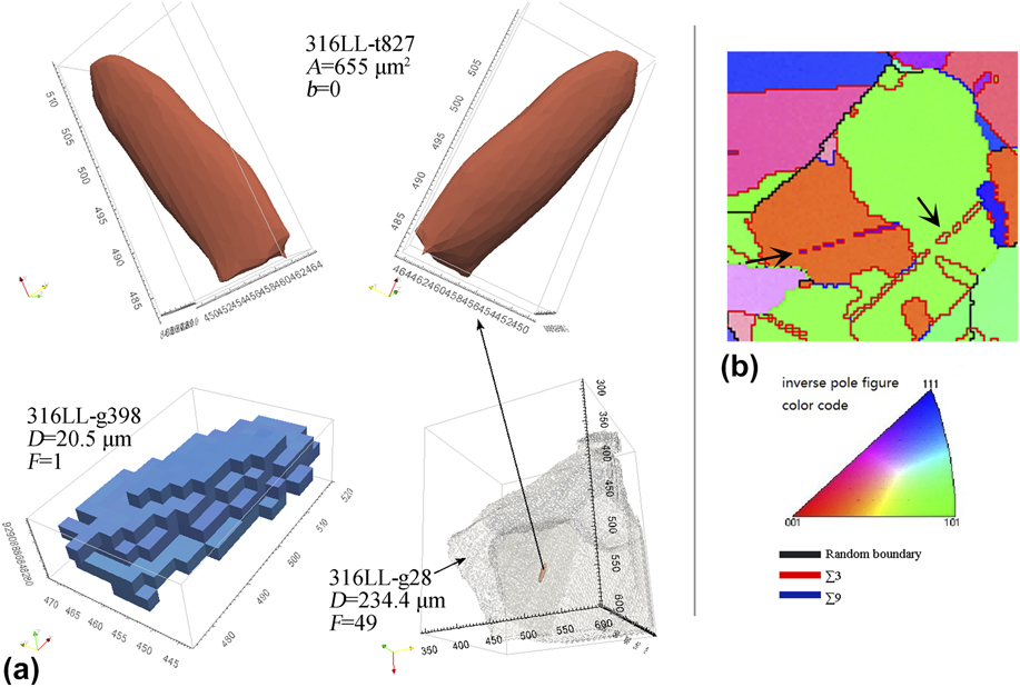
An example of occluded TB (type-C) is shown in Fig. 5(a). In a 2D section through the grain, it would appear as an island twin-grain. While island twin-grains can be observed frequently, it is quite less in these 3D microstructures. A reason is that the tunnel twins (type-B) and semiclosed tunnel twins (type-A) may be appeared as island twin-grains in 2D maps. Additionally, the thin plate-shaped twins may be segmented into several island twins (fragments) due to the coarse resolution in 2D maps, as shown in Fig. 5(b).
(a) Example of occluded TB (type-C) from sample 316LL. The island grain g398 locates in the center of outer grain g28. (See Fig. S1 in the Supplementary Material which is an u3d picture.) (b) Strings of observed occluded twins in a 2D EBSD map, but they actually should be fragments of a thin twin-grain.

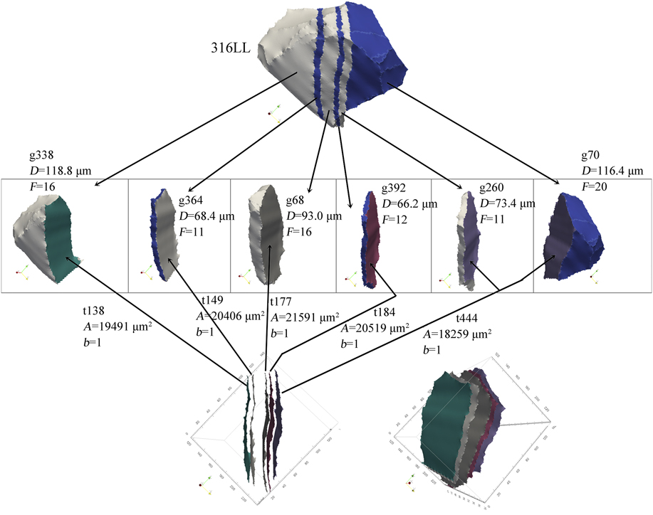
An example of parallel-multiplanar TBs (type-D) from specimen 316LL is illustrated in Fig. 6. While most of the observed type-D twins have two or three parallel TBs, Fig. 6 shows an assembly of five parallel planar TBs with similar areas. The equivalent circle diameters of the five TBs are about 160 μm. The thicknesses of the four lamellar twin-grains between the five TBs are in the range of 7–22 μm. There are many parallel-multiplanar TBs in the 3D microstructure of conventional 316L, but fewer are found in the GB-engineered 316L.
Example of parallel-multiplanar TBs (type-D) from sample 316LL, which is composed of five parallel TBs.

Some typical morphologies of twins and TBs are illustrated in Fig. 3 through Fig. 6. They were categorized into single-face TBs (type-A), tunnel TBs (type-B), occluded TBs (type-C), and parallel-multiplanar TBs (type-D), as defined in Fig. 2. Type-B TBs are the most common TBs in all three specimens (316LL, 316LS, and 316LGBE) on the basis of observation. The next most frequently observed are type-A and type-D TBs, and type-C TBs are rarely observed. Compared with conventional 316L, the GB-engineered 316L seemingly has fewer type-D and planar type-A TBs. In addition, while most TBs in the 3D microstructures of 316L before and after GB engineering could be classified into the four types defined in Fig. 2, some morphologically complex TBs were observed and it is difficult to classify them as any of the four types, especially in the GB-engineered sample.
B. Morphologically complex TBs
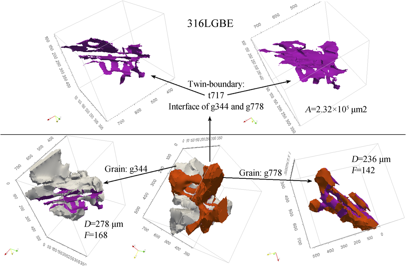
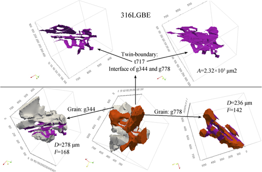
While the morphological features of simple TBs can easily be quantified or classified, some TBs in the GB-engineered 316L have very complex morphologies. An example of a TB with a complex morphology is shown in Fig. 7. It certainly has more than one hole so that it should be classified as type-B, but its extremely complex morphology distinguishes it from the others, especially when one compares it to the simple classifications that were developed on the basis of 2D observations.Reference Carpenter and Tamura1,Reference Mahajan, Pande, Imam and Rath2
Example of morphologically complex TB t717 from the GB-engineered 316L stainless steel, which is the interface of grains g344 and g778. Both two twin-grains have very complex morphologies (3D visualizations are shown in Figs. S2–S5 in the Supplementary Material).

It should be noted here that the entire interface between two neighboring grains was determined as a single boundary. The morphologically complex TB in Fig. 7 is the interface of grains g344 and g778 in sample 316LGBE. The two twin-grains also have very complex morphologies. Having many bar-shaped, lamellar-shaped and torus-shaped branches. The TB can be segmented into several simple segments, including parallel planar segments and tunnel-shaped segments. A reasonable suspicion is that this morphologically complex large twin-grain is not one grain but actually an assembly of several smaller grains that have been merged into the morphologically complex grain as a result of “clean-up” procedures that are used in the reconstruction of the 3D-EBSD data.Reference Groeber and Jackson44,Reference Groeber, Ghosh, Uchic and Dimiduk46,Reference Bhandari, Sarkar, Groeber, Uchic, Dimiduk and Ghosh48 In this context, it is important to mention here that the misorientation tolerance to identify grains is 15°. The TB and the two twin-grains shown in Fig. 7 before clean-up are shown in the Supplementary Material. The volume of grain g344 is 1.11 × 107 μm3 (1.13 × 107 μm3) before (after) clean-up, and the volume of grain g778 is 6.84 × 106 μm3 (6.86 × 106 μm3). The volumes of the two twin-grains changed little after clean-up, so post-processing of the 3D-EBSD data did not change the actual morphologies of the two grains. The morphologically complex twin-grains and TBs in Fig. 7 actually exist in the 3D microstructures, within the grain tolerance of 15°.
The cumulative distributions of the number and areas of TBs in the 3D microstructures of 316LS and 316LGBE are shown in Fig. S8 (see the Supplementary Material). About 62% (66%) of the TBs in 316LS (316LGBE) have small sizes that are less than the average TB size, but some TBs have areas that are more than four times the average. These large TBs have complex morphologies in general, such as TB t717 in Fig. 7, which is the largest area boundary (equivalent circle diameter 543.1 μm) in 316LGBE. The average diameter of TBs in 316LGBE (316LS) is 52.7 μm (33.8 μm). There are 1552 TBs in 316LS. Although only 0.9% of them have diameters that are more than four times the average, and their area fraction is about 11.6%. Comparatively, 316LGBE has 1393 TBs, and 1.5% of them have diameters that are more than four times the average, and the area fraction of these large TBs is about 26.7%. Therefore, morphologically complex TBs are observed more frequently in GB-engineered alloy 316L than in the conventionally processed alloy, and these boundaries are larger and more complex.
C. TB fractions in 3D microstructures
According to 2D studies, high fractions of TBs are a prominent characteristic of GB-engineered microstructures.Reference Michiuchi, Kokawa, Wang, Sato and Sakai5,Reference Liu, Xia, Li, Zhou, Bai, Su and Cai13–Reference Cao, Xia, Bai, Zhang, Zhou, Li and Jiang20,Reference Katnagallu, Mandal, Nagaraja, De Boer and Vadlamani22 The TB fraction can be measured as a length fraction or a number fraction from 2D maps. The length fraction is the most commonly used metric in 2D studies of GB-engineered materialsReference Michiuchi, Kokawa, Wang, Sato and Sakai5,Reference Liu, Xia, Li, Zhou, Bai, Su and Cai13–Reference Cao, Xia, Bai, Zhang, Zhou, Li and Jiang20,Reference Katnagallu, Mandal, Nagaraja, De Boer and Vadlamani22 ; number fraction statistics are rarely used.Reference Kumar, King and Schwartz28 The TB fractions determined from the three 3D microstructures considered here are shown in Fig. 8 and compared to the TB fractions determined from an arbitrarily selected 2D layer (the 40th) of each of the three materials. TB area fractions in the two conventional 316L samples, determined from the 3D data, are 39.8 and 42.9%. The TB area fraction in the GB-engineered sample is 58.7%. In comparison, the number fractions of TBs in 316LL, 316LS, and 316LGBE are 18.1%, 18.0%, and 19.8%, respectively. The TB area and length fractions increase after GB engineering and are greater than the number fractions in both the 3D and 2D statistics. However, the 3D data show that GB engineering has almost no effect on the number fraction, even though the 2D data show a considerable increase. These observations are explained by the very large and morphologically complex TBs that are detected in the 3D data as a single boundary but appear as disconnected separate boundaries in the 2D data.
Statistics of TB proportions in the 3D microstructures of specimens 316LL, 316LS, and 316LGBE, and in the 40th 2D-EBSD-slices of the three samples.

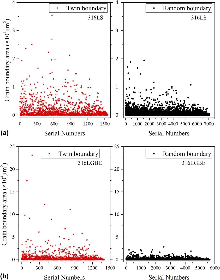
The areas of TBs in both GBE and conventional samples are, on average, larger than the random boundary areas. The average twin (random) boundary diameter in 316LGBE is 52.7 μm (23.3 μm), and in 316LS, it is 33.8 μm (18.4 μm). Figure 9 are scatter diagrams to show comparisons of TB areas and random boundary areas in samples 316LS and 316LGBE, in which the areas (Y-axis) are graphed with respect to an arbitrarily assigned serial number (X-axis). The correspondingly cumulative distributions are shown in Fig. S8 (see the Supplementary Material). Figure 9 obviously shows that 316LGBE has more large TBs when compared with 316LS. As a result, the GB-engineered sample has a higher area fraction of TBs while having roughly the same number fraction of TBs.
Statistics of boundary areas in the 3D microstructures of the conventional sample 316LS (a) and the GB-engineered sample 316LGBE (b). The TBs and random boundaries are illustrated, respectively. The horizontal-axis scale is corresponding to the boundary ID-numbers which are given each boundary randomly. There are 1552 (1393) TBs and 7072 (5660) random boundaries in 316LS (316LGBE).

IV. DISCUSSION
A. Occluded TBs
Bystrzycki et al.Reference Bystrzycki and Przetakiewicz35 believed that the occluded grains do not exist in 3D microstructures. However, 3D occluded twin-grains are really observed in this work, as illustrated in Fig. 5(a) (and Fig. S1 in the Supplementary Material). Somebody may be skeptical about the existence of real occluded twin-grains because the resolution of EBSD mapping can influence the observed grain morphology. This is especially true for thin plate-shaped twins which may be segmented into several fragments due to coarse resolution; examples of this phenomenon are illustrated in Fig. 5(b), where fragmented twins are indicated by the black arrows. What appears as a row of island twins would, almost certainly, appear as a large thin twin-grain if the EBSD step size was smaller.
However, this is not the case for the boundary illustrated in Fig. 5(a). In this case, the occluded twin-grain is located at the center of a large grain, and no other occluded grains were observed in the large grain. The occluded TB is the interface between the small grain and the large grain. The larger of the two grains has a grain diameter of 234.4 μm so the occluded twin-grain is far away from other grains. Although the occluded twin is small compared to the grain that surrounded it, it is comprised of 274 voxels and has a diameter of 20.5 μm, making it considerably larger than the resolution limit. Therefore, the occluded twin-grain in Fig. 5(a) is not likely to be a piece of a larger twin but is actually an occluded twin-grain. Although this shows that occluded twin-grains exist in 3D microstructures, we note that only a few were found and most of them are quite small. Because many island twin-grains are found in 2D maps, most of them are likely to be sectioning artifacts and in reality are pieces of other types of twins.
B. Improving intergranular properties by GB engineering
GB engineering has been proposed as a promising approach to improve the bulk properties and performance of polycrystalline materials without modifying the chemical composition. As discussed in many sources,Reference Michiuchi, Kokawa, Wang, Sato and Sakai5,Reference Liu, Xia, Li, Zhou, Bai, Su and Cai13–Reference Cao, Xia, Bai, Zhang, Zhou, Li and Jiang20,Reference Katnagallu, Mandal, Nagaraja, De Boer and Vadlamani22 the basic philosophy of GB engineering is to optimize the GB network by increasing the proportion of TBs. A high proportion of TBReference Michiuchi, Kokawa, Wang, Sato and Sakai5,Reference Liu, Xia, Li, Zhou, Bai, Su and Cai13–Reference Cao, Xia, Bai, Zhang, Zhou, Li and Jiang20,Reference Katnagallu, Mandal, Nagaraja, De Boer and Vadlamani22 is believed to be one of the prominent characteristics of GB-engineered microstructures compared with conventional microstructures. Past studiesReference Lin, Palumbo, Erb and Aust4–Reference Xia, Li, Liu and Zhou8 have shown that special boundaries, especially TBs, have greater resistance to intergranular degradation than random boundaries. However, the GB-sensitive properties of materials correlate more strongly with the topological characteristics of the entire GB network than with the proportions of certain boundary types. Whatever the concentration of TBs, they have a more favorable effect on properties when they disrupt the connectivity of random boundaries.Reference Michiuchi, Kokawa, Wang, Sato and Sakai5,Reference Kobayashi, Kobayashi and Watanabe17
The 2D GB network of 316LGBE, with the boundaries labeled by ∑, is shown in Fig. S9 (see the Supplementary Material). The low-∑ CSL boundary (3 ≤ ∑ ≤ 29) length fraction is 78.9% and the TB fraction is 68.9%. However, these special boundaries are not distributed randomly and form clusters (known as twin-related domains),Reference Liu, Xia, Li, Zhou, Bai, Su and Cai13,Reference Liu, Xia, Li, Zhou and Bai14,Reference Xia, Zhou and Chen19,Reference Gertsman and Henager23–Reference Lind, Li and Kumar26 resulting in a connected network of non-TBs (all types of high angle boundaries except ∑3) that persists in spite of the high fraction of TBs. Twin-related domains are found not only in 2D maps but were also found in a 3D study of the microstructure of copper before and after GB engineering.Reference Lind, Li and Kumar26 The non-TBs form a connected network of interfaces that separate the twin-related domains.
The GB-engineered sample has 5660 random boundaries, of which 5619 boundaries are connected in a continuous network. In comparison, the conventional sample has 7072 random boundaries, and 7070 of them are connected in a continuous network. 1370 TBs in 316LGBE are connected in a continuous network, and the other 23 do not connect with a TB. 1542 TBs in 316LS are connected in a continuous network, and the other 10 do not connect with a TB. In addition, the TB number fractions in triple junctions and quadruple junctions only have a slight increase after GB engineering.Reference Liu, Xia, Zhou, Bai and Rohrer33 Therefore, although the GB-engineered material has a higher TB area fraction, the random boundary connectivity persists.
From disrupting the random boundary connectivity, the number fraction of TBs is a more important metric than the area/length fraction. Percolation theory is a practical method to quantify the GB connectivity.Reference Michiuchi, Kokawa, Wang, Sato and Sakai5,Reference Kobayashi, Kobayashi and Watanabe17,Reference Tokita, Kokawa, Sato and Fujii31,Reference Frary and Schuh32 Schuh et al.Reference Frary and Schuh32 found that in 2D, the threshold number fraction of special boundaries to disrupt the random boundary connectivity is 0.35; in 3D, it is 0.775–0.85. Disappointing to some, the current 3D work finds that even though the GB engineering process created a high area fraction of TBs in the 316L stainless steel, the number fraction was slightly increased (see Fig. 8). The number fraction is much lower than the threshold predicted to break up the random boundary network. Some 2D studies also show that the TB number fraction is lower by 10–20 percentage points than the measured length fractions.Reference Randle and Coleman15,Reference Kumar, King and Schwartz28,Reference Randle51
In summary, the random GB network was not thoroughly disrupted after GB engineering although the TB area fraction increased significantly. The reason is that the TB number fraction increased by only a small amount. Large, morphologically complex TBs are responsible for the difference between the number and area fraction. New procedures for GB engineering should be developed in future to produce a high proportion of TBs not only in length/area but also in number. To reach the goal, it is necessary to understand the formation mechanism of the large morphologically complex TBs.
C. Formation mechanisms of TBs during GB engineering
As discussed above, the high area fraction of TBs in the GB-engineered 316L results from the formation of many large morphologically complex TBs that separate equally complex twinned grins (see Fig. 7). Although the formation of these twins or TBs is undesired, the formation mechanism is an interesting issue.
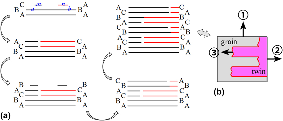
The formation of morphologically simple annealing twins has been studied for the past one hundred years, and several models had been proposed.Reference Carpenter and Tamura1,Reference Mahajan, Pande, Imam and Rath2,Reference Meyers and Murr34,Reference Fullman and Fisher52–Reference Gleiter57 However, these models do not address the formation of morphologically complex twins. The previous models for twin formation can be classified into two groups: (i) “growth accidents” due to a fault in stacking of atomsReference Carpenter and Tamura1,Reference Mahajan, Pande, Imam and Rath2,Reference Gleiter57 and (ii) “energetically driven processes” that alter the energy and mobility of the migrating boundaries at the recrystallization front.Reference Meyers and Murr34,Reference Fullman and Fisher52–Reference Field, Bradford, Nowell and Lillo56 The model proposed by GleiterReference Gleiter57 is schematically shown in Fig. 10(a). Atoms are emitted from a shrinking deformed grain onto a boundary step (ab, {111}-plane) of a growing grain. The newly formed lattice planes (the “two-dimensional nuclei” in Ref. Reference Gleiter57) are designated as m and n. The close-packed {111} plane has two types of interstices among the atoms, “△” and “▽”, so when an atom is emitted onto the {111} plane, it has two alternative ways to fit with the {111}-plane ab, i.e., stacking in sequence of “ABCAB C…” or “ABCAB A…”. The latter indicates a stacking fault, as shown by n in Fig. 10(a), which creates a TB. In the same way, 2D nucleation with the twinning orientation could form again and again, i.e., the multiple twinning process.Reference Xia, Zhou and Chen19,Reference Liu, Xia, Wang, Bai, Zhou and Su25,Reference Gottstein58–Reference Cayron60 As a result, a morphologically complex TB forms, as shown in Fig. 10(b). In other words, the morphologically complex large TB is a result of the merging of several small twins due to grain growth.
(a) Schematics showing the formation mechanism of the morphologically complex TBs during GB engineering. The lines indicate {111} planes. The red lines mean stacking faults. (b) Growth directions of the recrystallized twin-grain.

The attractive model proposed by Gleiter described the nucleation of twins by stacking faults or fault packets during recrystallization.Reference Gleiter57 Subsequently, the twin-grain could grow in three possible directions, as shown in Fig. 10(b). Following Gleiter’s model,Reference Gleiter57 the twin grows in direction-① which is perpendicular to the {111} plane; following Dash’s model,Reference Dash and Brown53 the twin grows in direction-② or ③ which are parallel to the {111} plane; MahajanReference Mahajan, Pande, Imam and Rath2 suggested that the twin grows in direction-②; MeyersReference Meyers and Murr34 and GoodhewReference Goodhew54 believed that the incoherent TB may move in direction-③. However, these models or growth directions are not incompatible. During GB engineering, the recrystallized twin-grains should grow along all the three directions. More twins could form in the wake of the grain growth in direction-①, which contribute to the complex morphology of the twins. The grain growth in direction-② and ③ contributes to the large size of the twins. Combination of the three growth models contributes to the formation of these morphologically complex large twins (TBs).
Regardless of the exact mechanism, a high frequency of twinning events, i.e., multiple twinning,Reference Xia, Zhou and Chen19,Reference Liu, Xia, Wang, Bai, Zhou and Su25,Reference Gottstein58–Reference Cayron60 occurs during GB engineering, but twins generated from a single parent grain (twins or twins of twins) may have the same orientation and may merge into a large twin, resulting in the formation of a morphologically complex large TB. However, the formation of these large TBs is not a desired result of GB engineering so the current GB engineering process should be modified to avoid this result.
Three types of thermomechanical processing are widely used for GB engineering: strain and annealing at high temperature for a short time,Reference Michiuchi, Kokawa, Wang, Sato and Sakai5,Reference Liu, Xia, Li, Zhou, Bai, Su and Cai13,Reference Liu, Xia, Li, Zhou and Bai14,Reference Liu, Xia, Li, Zhou and Bai24,Reference Liu, Xia, Wang, Bai, Zhou and Su25,Reference Deepak, Mandal, Athreya, Kim, Boer and Subramanya Sarma61–Reference Tan, Sridharan and Allen63 strain and annealing at a relatively low temperature for a long time,Reference Michiuchi, Kokawa, Wang, Sato and Sakai5,Reference Kobayashi, Kobayashi and Watanabe17,Reference Tokita, Kokawa, Sato and Fujii31,Reference Shimada, Kokawa, Wang, Sato and Karibe64 and repeated strain and annealing for several cycles.Reference Randle and Coleman15,Reference Kumar, King and Schwartz28,Reference Telang, Gill, Kumar, Teysseyre, Qian, Mannava and Vasudevan36,Reference Randle and Jones62,Reference Tan, Sridharan and Allen63 The first type was used in this work, and it is an economical method compared to the other two methods and suitable for industrial application. In general, long annealing times or iterative thermomechanical processing could produce a higher proportion of TBs. However, based on the microstructures illustrated in Refs. Reference Randle and Coleman15, Reference Kobayashi, Kobayashi and Watanabe17, and Reference Telang, Gill, Kumar, Teysseyre, Qian, Mannava and Vasudevan36, these two methods do not prevent the formation of the morphologically complex TBs. Therefore, although most papers on GB engineering equate success with developing a high area/length fraction of special boundaries, developing a new procedure that could increase the number fraction is still important in future from the perspective of disrupting the random boundary connectivity.
V. CONCLUSIONS
The morphology, connectivity, and TB fractions in a GB-engineered austenitic stainless steel have been measured from 3D microstructure data and compared with those of conventional samples of the same material. The main findings are as follows:
(1) Morphologically simple TBs can be classified into four categories: (type-A) single-face TBs, (type-B) tunnel TBs, (type-C) occluded TBs, and (type-D) parallel-multiplanar TBs. In the order of most to least common, are TBs of type-B, type-A, type-D, and type-C. This order is found in both the conventional and GB-engineered samples. The GB-engineered sample has a higher fraction of type-B TBs and a lower fraction of type-D TBs than the conventional sample.
(2) Compared with the conventional samples, a prominent characteristic of the GB-engineered microstructure is the formation of some large and morphologically complex TBs. This leads to a higher area fraction of TBs in the GB-engineered sample. However, the number fraction of TBs in the GB-engineered sample is not significantly different than the conventional sample. The connectivity of random boundaries (or non-TBs) was not disrupted thoroughly by GB engineering.
Supplementary Material
To view supplementary material for this article, please visit https://doi.org/10.1557/jmr.2018.133.
ACKNOWLEDGMENTS
This work was supported by the National Natural Science Foundation of China (Grant Nos. 51671122 and 51701017) and the Fund of Jiangsu Province for the Transformation of Scientific and Technological Achievements (BA2017126).