Introduction

Ice streams have long been recognized as important to the evolution of the West Antarctic ice sheet (WAIS), not only for their possible instability but also because their flow is the main mechanism by which ice is transferred from the inland reservoir of the ice sheet to the Ross Ice Shelf. The locations of ice-stream ˚onsets", the points of transition from inland to ice-stream flow, have recently become a focus of research (Reference Anandakrishnan, Blankenship, Alley and StoffaAnandakrishnan and others, 1998; Reference BellBell and others, 1998; Bindschadler, in press). A new, sweeping view of ice flow in West Antarctica shows that the transition includes not only the onsets themselves but networks of fast-flowing tributaries that direct ice toward the ice-stream onsets (RADARSAT-derived interferometry of Reference JoughinJoughin and others, 1999). The velocity observations in West Antarctica are exceptional in their detail. Furthermore, high-resolution measurements of ice thickness have been made in much of the area they cover. We use a combination of the RADARSAT-derived velocities and measurements of ice-sheet geometry (Reference Bamber and BindschadlerBamber and Bindschadler, 1997; D. Blankenship, unpublished data) to investigate the extended transition from inland to ice-stream flow represented by the pre-ice-stream tributaries flowing in the catchment area of Ice Streams D and E.

Observations

Ice flow follows a complicated network of tributaries into Ice Stream D and into the southern side of Ice Stream E (Fig. 1). We do not classify these features as ice streams, because tributary speeds are relatively slow while driving stress is relatively large. The larger of two main tributaries flowing into Ice Stream D, labelled "Dl" in Figure 1, diverts from a tributary flowing down the Bentley Subglacial Trench into a shallower subglacial valley (× = –900, y = –500 in Fig. 1). Downstream, the shallower valley becomes the main branch of Ice Stream D. A second tributary feeding Ice Stream D, labelled "D2" in Figure 1, emanates from the same source region (× = –900, y = –650) as tributaries to the southern side of Ice Stream E. The Ice Stream E tributaries are labelled "El" and "E2" in Figure 1. Surface speeds in the tributaries are tens of meters per annum. Within the tributaries, ice speed does not increase continually with distance downstream, as would occur in an ice stream. Instead, ice speed increases and decreases in a spatial pattern that in most places mimics the basal topography (Fig. 2).

Fig. 1.

Ice-surface speed in the Ice Stream D and E tributary area. The contour interval is 20ma^–1 from 0 to 100, and 100 m a’¹ thereafter. The color map delineates the boundaries of the velocity dataset, with dark-blue colors representing speeds near zero, and speeds over 200 m a^–1 saturating as dark red. Tick marks along the edges of the map are in km, with the origin at the South Pole. Flow features corresponding to the Bentley Subglacial Trench, Ice Streams C and D and the _Pre-ice-stream tributaries Dl, D2, Eland E2 are identified. The exterior boundary of the numerical model is plotted with a short dashed line. Long dashed lines trace the transects in Figures 2 and 3. The divide between ice flowing toward the Ross Ice Shelf and toward the Ronne Ice Shelf is to the right and upper right (west and south), and surface slope is generally from the upper right toward the lower left of the map region. An approximate map location is shaded in grey in the inset drawing of Antarctica. The tributary data are from Joughin and others (in press) and Reference Chen, Bindschadler and VornbergerChen and others (1998), and velocities in the main trunk of Ice Stream D are provided by the Earth Observing System Distributed Active Archive Center at the National Snow and Ice Data Center, University of Colorado, Boulder, U.S. A.

It is instructive to compare the characteristics of tributaries D1 and D2. The onset of fast ice-stream-style flow within the D1 tributary is the most intensely studied of any ice-stream onset. A large-area network of surface markers was installed in the region of the Dl-to-D onset to observe the flow transition (Reference Chen, Bindschadler and VornbergerChen and others, 1998). In that area, concurrent gradual downstream increases in driving stress and ice speed culminate at what has been defined as the onset location, where driving stress reaches a maximum (at about × = –850, y = –575 in Fig. 1 and at 215 km in Fig. 2; cf Bindschadler, in press). The driving-stress maximum occurs at the downstream end of the thickest reach of the tributary after its diversion from the Bentley Subglacial Trench. Downstream of the Dl-to-D onset, driving stress decreases rapidly while ice speed continues to increase. The pattern of flow down tributary Dl is straightforward, fitting the general understanding of the profound difference between inland ice-sheet dynamics and ice-stream dynamics (Reference RoseRose, 1979; Reference BentleyBentley, 1987; Bindschadler, in press). The pattern of flow down the tributary D2 is quite different. Ice speed remains fairly constant with distance downstream, at 50–100 ma^–1. While D2, like other tributaries in the area, has a driving-stress maximum along its course, there is only a modest increase in speed downstream of that maximum (at about × = –850, y = –650 in Fig. 1 and at 75 km in Fig. 2).

Fig. 2.

Downstream profiles through tributaries Dl and D2, showing ice surface and bed elevation, magnitude of driving stress averaged over 20 ice thicknesses, observed ice speed, a comparison of modelled and observed ice speed within the model domain and the magnitude of the hydraulic potential gradient within the model domain. Solid lines denote observed surface speed, and long and short dashed lines denote speed computed by the warm- and cold-ice models, respectively. The Dl profile passes through the Ice Stream D onset and down several hundred kilometers of the ice stream. The D2 profile ends just after entering the shear margin of Ice Stream D (at about x= –650, y = –700 in Fig. I). Profiles of model-derived quantities end at the edge of the model domain. The abscissa marks distance along each profile, in km. Driving stress is computed as the product of ice density, the acceleration due to gravity, ice thickness and the sine of the surface slope.

Differences between the two tributaries flowing toward Ice Stream D must be due to differences in their physical settings. One possibility is the geometries of the subglacial valleys in which they flow. The valley beneath Dl is generally wider and deeper than the valley beneath D2. Another possibility is related to ice thickness. Ice in the Dl tributary is thicker and likely warmer at depth than D2 ice. Thus basal shear, which is responsible for most of the deformation flow, is larger in Dl than in D2. Causes for inter-tributary variations that are more difficult to investigate with the present datasets he in the nature of the subglacial water drainage, till-water content or thickness, or bedrock type.

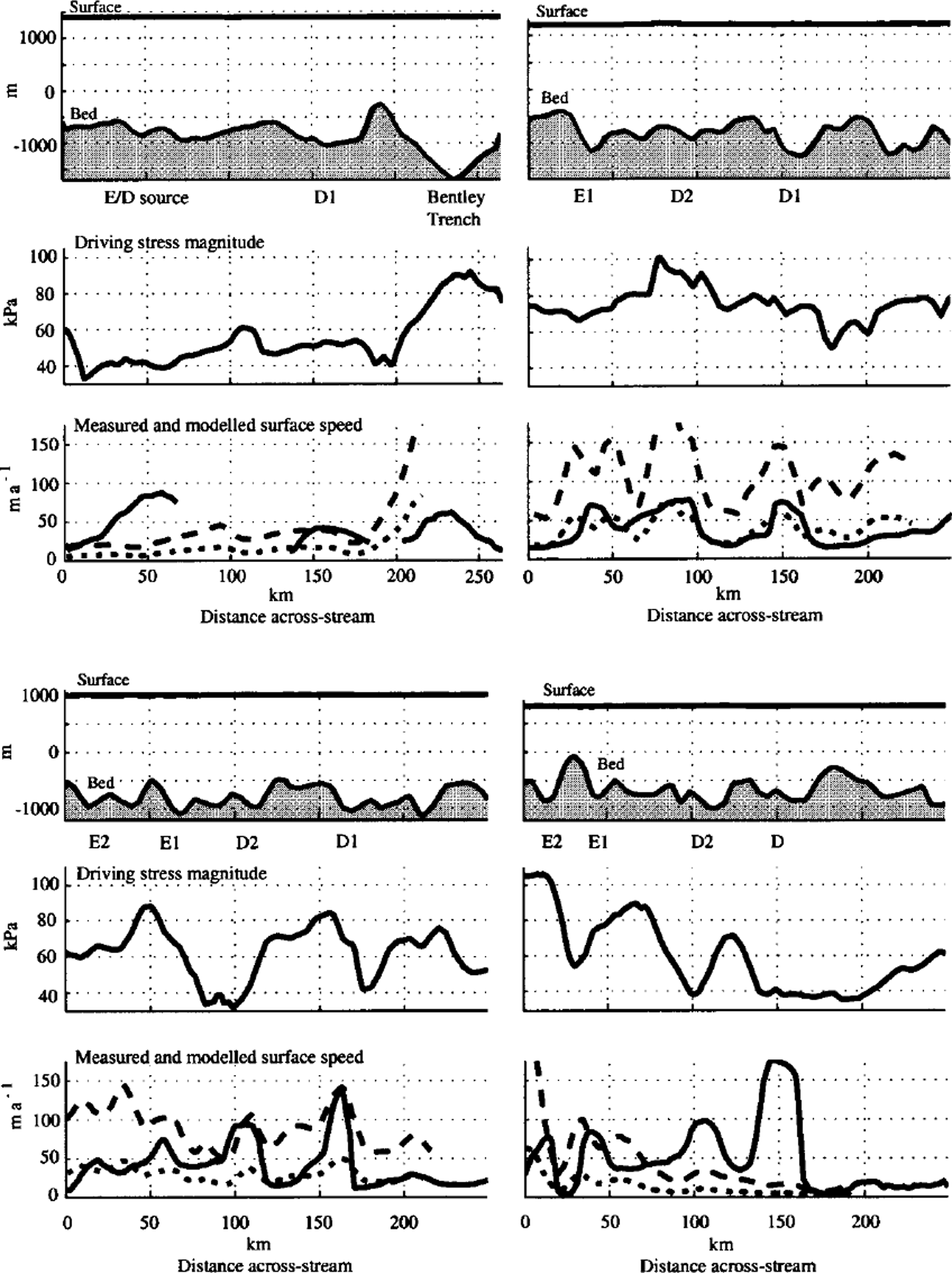
The pre-ice-stream tributaries tend to follow valleys in the basal topography Reference JoughinJoughin and others, 1999). This is sensible, as the greater ice thickness over subglacial valleys will yield faster internal deformation and thus faster ice flow (Fig. 3). However, not all subglacial valleys host fast-flowing tributaries. The Figure 3 cross-sections through several tributaries show intervening valleys that do not contain distinct concentrations of fast ice flow. Thus, it is likely that ice thickness is not the only contributor to the fast ice flow. Understanding the processes of tributary flow requires a combination of geophysical soundings (cf Reference Anandakrishnan, Blankenship, Alley and StoffaAnandakrishnan and others, 1998; Reference BellBell and others, 1998) and numerical modelling. We begin that effort with a series of forward models that evaluate the relative contributions of ice thickness and temperature, and by inference ice sliding, to the observed tributary flow.

Fig. 3.

Profiles that cross tributaries El, E2, Dl and D2, along four different surface-elevation contours, 1400,1200,1000 and 800 m, so that ice flow is toward the observer. Top panels show ice surface and bed elevation, middle panels show the magnitude of driving stress averaged over 20 ice thicknesses, and bottom panels show surface ice speed. Solid lines denote observed speed, and long and short dashed lines denote speed computed by the warm- and cold-ice models, respectively. Gaps in the observed surface speed along the 1400 m elevation contour correspond to gaps in the RADARSATdata coverage. Driving stress is computed as the product of ice density, the acceleration due to gravity, ice thickness and the sine of the surface slope.

Numerical Model

We simulate present-day ice flow using a quasi-three-dimensional thermodynamic/dynamic numerical model of the ice sheet. Ice velocity and temperature are computed using balance equations, embodied as piece-wise linear functions in a finite-element mesh. The model domain encompasses a network of associated tributaries flowing into Ice Stream D and the southern side of Ice Stream E (the outline of the domain is shown in Figure 4). The area of the model is limited so that its resolution can be fine enough to capture small-wavelength features of the bedrock topography. Its shape makes best use of a high-resolution ice-thickness dataset (D Blankenship, unpublished data). The model mesh contains 5872 horizontal triangular elements and 26 vertical layers, 5 of which represent the bedrock below the ice sheet. Horizontal resolution is about 5 km and the mean element area is about 12 km². Vertical resolution varies, being finest near the base of the ice sheet.

Fig. 4.

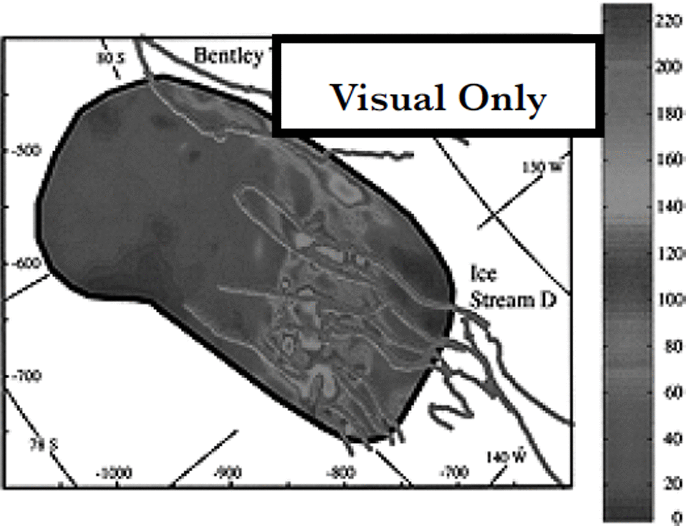
Ice-surface speed as computed by the warm-ice model. The exterior boundary of the model domain is marked by a heavy black line. Prominent tributary boundary contours from Figure 1 are marked with heavy grey lines. The boundaries may be used to identify the tributaries and as a reference for comparison with Figure 1. The map area, to which meridians and parallels have been added for help in locating the study area, is nearly the same as in Figure 1.

The stress-balance equations are similar to those employed by numerous authors (cf. Reference HuybrechtsHuybrechts, 1990). Their derivation makes use of the shallow-ice approximation, the assumption that ice is incompressible and Glen’s flow law for ice. For example, the expression for horizontal velocity, u, in one direction is:

where ω lies in the × direction of a Cartesian coordinate system, z is the vertical coordinate, the basal elevation, z_b is the difference between the top surface elevation, z_s, and the ice thickness, p is ice density, g is the acceleration due to gravity, A is the temperature-dependent rate factor for ice deformation by dislocation creep, and the flow-law exponent n is 3 (Reference HookeHooke, 1981). A similar expression is written for velocity in the other horizontal direction. Because the resolution of the model mesh is not very different from the ice thickness in the study area, the driving stress must be averaged over many ice thicknesses before it is used to compute ice velocity (Reference PatersonPaterson, 1994, p. 98–101). Here, the integral in Equation (1) is averaged over a radius often ice thicknesses, using a simple moving-mean calculation. We do not include a sliding parameterization, so that spatial variations in the physical setting are not obscured (in other whole-ice-sheet models, horizontal velocity is usually augmented where the ice/bed interface reaches the melt temperature; cf. Reference PaynePayne, 1995; Reference HulbeHulbe, 1998). The result is that mismatch between modelled and observed ice velocity can be used to infer ice sliding. Vertical velocity is computed according to ice divergence due to horizontal motion, the rate of new ice accumulation on the upper surface, melting at the bottom surface and flow along the bed slope. A full description of the equations is given in Reference HulbeHulbe (1998).

The stress-balance equations require ice-sheet surface elevation and thickness, vertical velocity conditions at the top and bottom boundaries and an estimate of the flow-law rate factor, A. Present-day surface elevation is interpolated to model mesh nodes from the digital elevation model of Reference Bamber and BindschadlerBamber and Bindschadler (1997), and smoothed by averaging over a radius often ice thicknesses. Ice thickness, and thus bedrock topography, is derived from a high-resolution airborne radar survey (D. Blankenship, unpublished data from Support Office for Aerogeophysical Research). The surface accumulation rate is specified using present-day observed accumulation rates compiled by the British Antarctic Survey (Reference Vaughan, Bamber, Giovinetto, Russell and CooperVaughan and others, 1999). The basal melting rate is computed according to heat continuity in the model domain. The magnitude of the flow-law rate factor is difficult to estimate because few measurements of ice temperature have been made in West Antarctica. A spatially constant rate factor can be used, assuming some standard value or a value derived from temperature measurements in the Byrd station ice core, the only measured ice temperature within the model domain. Alternatively, a thermodynamic model can be used to estimate ice temperature and thus a spatially variable rate factor. The third method is preferred, because it accounts for spatial variations in ice thickness and surface accumulation rates, both of which have a strong influence on ice temperature.

Temperature is computed according to heat balance in the ice and an underlying bedrock layer (cf Reference PaynePayne, 1995; Reference HulbeHulbe, 1998). The balance equations include advective and diffusive terms in the ice,

and a diffusive equation in the bedrock,

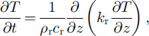
where T is temperature, t is time, c is heat capacity, k is heat conductivity, W is viscous heating due to ice flow, and the subscript "r" denotes a bedrock value. The bedrock equation is solved between the bedrock surface, z_τ, and a fixed depth, 750 m below that surface. A geothermal flux of 0.0669 W nT² (Reference Budd, Jenssen, Van der Veen and OerlemansBudd and Jenssen, 1987) is applied as a boundary condition at the base of the bedrock layer. The upper surface boundary condition is specified using temperature derived from infrared temperature (Reference ComisoComiso, 1994). The horizontal and vertical parts of Equation (2a) are solved separately (thus the model is ˚quasi-three-dimensional").

The limited extent of the model domain creates special considerations in selecting advective boundary conditions for the heat-balance equations. The domain is embedded within a complicated flow field, which depends in part on ice temperature. Thus, it is difficult to determine a priori horizontal-velocity boundary conditions. Additionally, vertical temperature conditions must be specified where ice advects into the model domain. Here we take advantage of the circumstance that in most locations where ice flow is into the domain, the rate of flow will be small, ω10 m a^–1, and set the velocity boundary condition to zero, obviating the need for a temperature boundary condition. This condition is most incorrect along the southwestern corner of the model domain, where warm, thick ice from the Bentley Trench flows into the domain and may cause the model to underestimate ice temperature there. In effect, at boundaries where horizontal ad-vection is ignored, the model will compute a temperature profile that balances vertical flux terms only.

Steady-state ice temperature for the selected model domain and boundary conditions is computed by iteration of the heat-balance portion of the model. The initial temperature condition is interpolated to the horizontal and vertical mesh nodes from the steady-state solution of a previous model experiment that encompassed the entire Ross Ice Stream catchment basin (Reference HulbeHulbe, 1998). An initial estimate of horizontal velocity, made using a constant rate factor A = 1 ×10–16Pa-3a–1⁶ , is used to compute advective terms. To reduce noise in the temperature fields resulting from poor knowledge of horizontal strain rates (Reference HulbeHulbe, 1998), early stages of the thermal spin-up use a vertical velocity, w, that includes only the surface accumulation rate and the basal melting rate. The iteration proceeds until the mean rate of change of temperature at any vertical node within the model domain is ω1 × 10^––4% a^–1. Comparison of model-computed and observed temperature near the site of the Byrd station borehole (at 80° S, 120° W; e.g. Reference WhillansWhillans, 1977) shows that the model overestimates temperature at mid-depth by as much as 5 K. The comparatively warmer temperatures arise from ice thickness at the selected model mesh node that is about 250 m greater than the measured borehole thickness, from the lack of cold-ice advection into the area from higher elevations, and from the tendency of the simple thermal spin-up to enhance the feedbacks among ice temperature, viscous heating and the deformation rate (Reference HulbeHulbe, 1998). However, the difference in temperature in the bottom 25% of the ice, where most of the shear deformation occurs, is small, ω1 K. The model is likely to overestimate ice temperature in some locations (especially where surface slope, and thus internal deformation, is large), but because our goal is simply to improve on the very limited knowledge of ice temperature in the area, we accept the error.

Numerical Experiments

We use the numerical model to compute two ice-flow fields. In the first, both surface slope and ice thickness influence ice flow, but the effect of ice temperature is minimized by assuming a constant rate factor of A = 1 × l0^–16 Pa^–3 a^–1. This is equivalent to assuming a uniform, cold ice temperature (we refer to this as the ˚cold" model). In the second experiment, we use a spatially varying, linear depth-average rate factor computed using the temperature field from the thermal spin-up of the model domain (the ˚warm" model). The depth-average value is used to mitigate errors in the vertical temperature distribution (as discussed above). The estimates of ice velocity provide a range in which ice thickness and temperature alone may be sufficient to cause the observed ice flow. Where measured velocity exceeds the modelled velocity, sliding at the ice/bed interface is indicated.

The two modelled flow fields differ in magnitude but have many common spatial characteristics. The result of the second (variable rate factor) model is shown in Figure 4. As can be anticipated from the driving-stress plots in Figure 2, the tributaries all contain velocity maxima that coincide with driving-stress maxima. The maxima follow an arc in surface slope (and thus driving stress) around the Ross Ice Stream catchment basin, that has been noted by several authors (Reference RoseRose, 1979; Reference BentleyBentley, 1987; Reference BellBell and others, 1998). Downstream of the maxima, model-computed ice speed decreases. That pattern agrees with the observed pattern along tributaries D2, El and E2, where ice slows and then speeds again, although the spatial agreement is only approximate. The speed increase farther downstream along D2, El and E2 is not reproduced. That failure of the inland equations suggests an increased role for longitudinal stresses with proximity to the ice-stream onset. Even less agreement exists along the main trunk of Ice Stream D. That is expected, as the standard inland ice-sheet dynamics is insufficient to simulate true ice-stream flow.

Sliding at the ice/bed interface is indicated where our model underestimates ice speed, because it assumes no contribution to ice flow from sliding. Surface speeds for both models are plotted along the downstream and across-stream profiles in Figures 2 and 3. Imprecision in the flow law for ice or errors in our selection of the rate factor must account for some disagreement between observation and calculation. Indeed, our temperature estimates are likely warmer than the real ice sheet, and result in overestimates of ice speed in some locations. Nevertheless, where observed ice speed is significantly larger than the modelled ice speed, sliding must play a dominant role in ice flow. Where our cold and warm models bracket the observed speed, sliding may make no contribution or some contribution to ice motion.

The contrast between the two tributaries flowing toward Ice Stream D is striking. In the far upstream reach of the Dl tributary, sliding is either absent or makes a small contribution to ice motion (0–125 km in Fig. 2, column 1). Nearer to the onset of Ice Stream D (125–215 km in Fig. 2, column 1) sliding becomes relatively more important. Note that the warm model probably overestimates temperature in this region because surface slope is relatively large. The model does not simulate fast ice-stream flow, so downstream of the onset, ice speed is underestimated. The pattern of change along the D2 tributary is quite different from the pattern along Dl. At the far upstream end of D2 (0–60 km in Fig. 2, column 2), in a source region shared with several tributaries to Ice Stream E, both the warm and cold models underestimate ice speed substantially (by up to 85%). Sliding is likely to be very large in that area. Farther downstream, the magnitude of sliding appears to vary, first decreasing (60–150 km in Fig. 2, column 2) and then increasing. Ice at the downstream end of the profile speeds suddenly as it enters the shear margin of Ice Stream D.

Profiles of observed and modelled surface speed across the tributaries demonstrate several features of tributary flow (Fig. 3). First, the contrast in the downstream pattern of sliding for the two tributaries leading to Ice Stream D is quite clear. The profile at 1400 m elevation crosses the upstream ends of Dl and the shared source region for several Ice Stream D and E tributaries. The models underestimate surface speed substantially in the Ice Stream E/D source area but provide better estimates for tributary Dl, implying substantial sliding in the former location and no sliding in the latter. Farther downstream, along the 1200 and 1000 m elevation profiles, the importance of sliding beneath Dl increases (the onset to Ice Stream D is just downstream of the 1000 m elevation contour; see Fig. 2; Reference Chen, Bindschadler and VornbergerChen, and others, 1998; Bindschadler, in press) while sliding at the base of D2 appears to first decrease and then increase with distance downstream. The tributaries to Ice Stream E also exhibit an irregular pattern of large and small motion from sliding. Second, while the tendency is for subglacial valleys to host fast-flowing tributaries, the across-flow profiles show that not all valleys induce tributary flow (e.g. the valleys at 70 km in Fig. 3, column 2, part 1, and at 40 km in Fig. 3, column 1, part 2). Third, driving stresses are relatively large where the profiles cross tributaries, an observation that influences our interpretation that tributary flow is distinct from ice-stream flow.

Discussion

Significant flow enhancement is suggested where the models underestimate ice speed. Basal melting rates, computed in the thermal spin-up of the model domain, are small throughout most of the Ice Stream D and E tributary region, with larger rates along some subglacial valleys (Fig. 5). The tops of ridges between valleys tend to freeze. Limitations inherent to the heat-balance calculation make the exact magnitudes of the melting rates meaningless (the mean melting rate is 1.9 mm a"¹), but the regional pattern of melting and freezing is robust, given limitations in knowledge of the geothermal flux (a discussion can be found in Reference HulbeHulbe, 1998). Where melting rates are large, abundant water may promote basal sliding by increasing basal water pressure if the water is stored (Reference Fowler and JohnsonFowler and Johnson, 1995), or perhaps by reducing the strength of the subglacial till (Reference TulaczykTulaczyk, 1998). The magnitude of the hydraulic potential gradient along the Ice Stream Dl and D2 tributaries is plotted in Figure 2 (calculated as the gradient of pgh + ρ_wgz_b, where ρ^w is the density of fresh water and h is the ice thickness). Where the gradient is large, basal water will tend to be driven down-gradient, while in areas where the gradient is small, the possibility exists for water storage (and thus ice sliding). In general, gradients are smaller in areas where the observed and modelled speeds differ most. For example, the magnitude of the hydraulic potential gradient along the upstream, probably sliding, end of the D2 tributary (0–50 km in Fig. 2, column 2) is about 40% smaller than the gradient farther downstream. The correlation is not conclusive, because downstream changes in subglacial rock type, valley width or bed roughness could also cause the observed flow pattern, but it does fit with our inferences from the ice-sheet model.

Fig. 5.

Map of the tendency toward basal melting or basal freezing, computed by the thermodynamic model. Areas in white tend to freeze, and areas in grey tend to melt, with darker colors representing greater melting rates. The mean melt rate in the model domain is 1.9 mm a’¹ . Contours are 1.0 mm a–₁. The most notable attribute of the basal melting field is the tendency toward freezing between pre-ice-stream tributaries. Those areas correspond to ridges in the subglacial topography.

Conclusion

A widespread network of tributaries flowing toward the recognized onsets of WAIS ice streams was recently discovered by means of RADARSAT interferometry (Joughin and others, in press). Our goal in developing the model described here was to determine if the tributaries are governed by inland or ice-stream-style dynamics and to explore the influence of physical attributes of the study area on tributary flow. We find no simple pattern of change in the ice flow with distance downstream, but instead a pattern of relatively more and less sliding that is likely related to the abundance of subglacial meltwater. Other possible contributions to the spatial variability of tributary flow, from variations in basal till or perhaps even ice-crystal fabric, cannot be eliminated by the analyses presented here. Basal properties may be better illuminated by inverse calculations, guided by insights from the present work. Inversion of the observed surface velocity and ice thickness has proved challenging, due to offsets between the kinematic center lines of tributaries and the thalwegs of some subglacial valleys and uncertainties in the ice temperature.

The observed flow variations are smoother than variations predicted by the standard inland ice-sheet stress-balance equations. That is, to some degree the stress-balance equations fail. Variations in basal properties or ice rheology may not be the only cause of mismatch between the observed and modelled flow. It is possible that tributary flow represents a long transition in which longitudinal stresses are relatively more important than in inland-style flow but less important than in ice-stream flow.