


1. Introduction
An important and well-developed class of stochastic control problems is related to optimal stopping time. The goal is to find times at which an underlying stochastic process Z should be stopped in order to optimize the values of some given functional of interest. Essentially, the optimal stopping time problem is completely described by the so-called supermartingale Snell envelope
 $$
\begin{equation}
S(t)\quad{\rm{: = }}\mathop {{\rm{ess sup}}}\limits_{_{\tau \ge t}} {\rm{ E}}[Z(\tau )\mid {{\cal F}_t}],\quad 0 \le t \le T,
\end{equation}
$$
written with respect to (w.r.t.) a given filtration
 $\mathbb{F}=(\mathcal{F}_t)_{0\le t\le
T}$
, where ess sup in (1) is computed over the class of all
 $\mathbb{F}$
stopping times located on [t,T]. The literature on probabilistic techniques in optimal stopping problems is vast. We refer, for instance, to the expositions of [Reference Carmona, Del Moral, Hu and Oudjane14, Reference Lamberton25] and other references therein for a broad overview of the techniques in this area.
One typical approach in solving an optimal stopping time problem is to discretize the Snell envelope (1) along a discrete time period
 $t_0, \ldots, t_p$
by means of Euler-type discretization schemes. The main obstacle is the obtention of continuation values (expressed as
 $\mathcal{F}_{t_i}$
-conditional expectations) in the dynamic programming algorithm. In this case, least-squares Monte Carlo methods can be employed by using non-parametric regression techniques based on a suitable choice of regression polynomials (see, e.g., [Reference Zanger33] and other references therein). Another popular approach is to make use of some available representations for conditional expectations in terms of a suitable ratio of unconditional expectations obtained by using Malliavin calculus (see, e.g., [Reference Bouchard and Touzi11]). These approaches work well as long as one may reduce the information flow
 $$({{\cal F}_{{t_i}}})_{i = 0}^p$$
by a finite-dimensional random vector
 $X(t_0), \ldots, X(t_p)$
. This is only possible if the state is Markovian. Otherwise, the computation of continuation values is a priori unfeasible from a computational point of view. A dual approach studied in [Reference Rogers31] has also been investigated by many authors (see, e.g., [Reference Belomestny5] and other references therein). In this approach the key step is to find the ‘optimal’ martingale, and the importance of the Markov property seems critical to obtain concrete basis functions to parameterize martingales (see, e.g., [Reference Belomestny5, Reference Schoenmakers, Zhang and Huang32]).
Beyond Markovian state processes, one approach consists in expressing the Snell envelope S as the unique solution of a reflected backward stochastic differential equation (BSDE). On one hand, at a representation level, the theory of reflected BSDEs characterizes the semimartingale structure of S in full generality. On the other hand, concrete methods to compute martingale representations are restricted to the Markovian case (see, e.g., [Reference Bally and Pagès2, Reference Bally and Pagès3, Reference Bouchard, Warin, Carmona, Del Moral, Hu and Oudjane12, Reference Bouchard and Chassagneux10]). More recent approaches based on path-dependent partial differential equations (PDEs; see, e.g., [Reference Ekren17]) yield differential representations of the Snell envelope (even in the fully nonlinear case) under pathwise regularity on the obstacles related to the reflected BSDE. We also emphasize the recent representation result in [Reference Fuhrman, Pham and Zeni20] for the Snell envelope in terms of true BSDEs, defined on an enlarged probability space, containing a jump part and involving sign constraints. We observe that the use of reflected BSDEs and path-dependent PDEs to solve concretely the optimal stopping problem beyond the Markovian case seems to be a very hard task. The key difficulty is that solving an optimal stopping time problem for a fully non-Markovian state is essentially a stochastic optimal control problem driven by an infinite-dimensional state.
Optimal stopping time problems based on reward path-dependent functionals of fully non-Markovian states arise in many applications and it remains a challenging task to design concrete ways of solving them. One typical example is the problem of pricing American options written on stochastic volatility models (X,V) where the volatility variable V is a functional of fractional Brownian motion (FBM) with long-range dependence (see, e.g., [Reference Chronopoulou and Viens15] and other references therein) or short-range dependence as recently observed by many works (see, e.g., [Reference Bayer, Friz and Gatheral4, Reference Forde and Zhang19, Reference Gatheral21] and other references therein). In this case one cannot interpret (X,V) as an ‘augmented’ finite-dimensional Markov process due to nontrivial correlations associated with FBM and hence a concrete solution of the related optimal stopping problem is very challenging. We stress that even optimal stopping problems based on finite-dimensional ‘augmented’ Markovian-type models (X,V) (e.g. Cox–Ingersoll–Ross-type models driven by Brownian motion) are not easy to solve (see, e.g., [Reference Agarwal, Juneja and Sircar1, Reference Rambharat and Brockwell30]). In practice, the volatility V is not directly observed so that it has to be approximated. If the volatility is estimated with accuracy, then standard Markovian methods can be fairly implemented to solve the control problem. Otherwise, the optimal stopping problem is non-Markovian.
The goal of this paper is to present a systematic method of constructing continuation regions and optimal values for optimal stopping problems based on arbitrary continuous reward processes Z. We are particularly interested in the non-Markovian case, i.e.
 $Z = F(X)$
where F is a path-dependent functional of an underlying non-Markovian continuous process X which is adapted to a filtration generated by a d-dimensional Brownian motion B. In our philosophy, the reward process Z is viewed as a generic non-anticipative functional of B, i.e.
 \begin{equation}
B\mapsto Z(B)
\label{eqn2}
\end{equation}
rather than X, and it may possibly be based on different kinds of states not reducible to vectors of Markov processes: solutions of path-dependent stochastic differential equations (SDEs), processes involving fractional Brownian motions and other singular functionals of Brownian motions.
The methodology is based on Leão and Ohashi [Reference Leão and Ohashi26] and Leão, Ohashi, and Simas [Reference Leão, Ohashi and Simas27], who showed very strong continuity/stability of a large class of Wiener functionals (2) w.r.t. continuous-time random walk structures
 ${\cal D}$
driven by suitable waiting times
 $T^k_n;\,\,n,k\ge 1$
(see (4) and (5)) which encode the evolution of the Brownian motion at small scales
 $\varepsilon_k\downarrow 0$
as
 $k\rightarrow +\infty$
. Here,
 $\varepsilon_k = \varphi(k)$
for a strictly decreasing function with inverse
 $\xi$
. The main idea is to reduce the dimension by discretizing the Brownian filtration at a given time t by
 $${\cal F}_t^k: = \{ \bigcup\limits_{j \ge 0} {{D_j}} \cap \{ T_j^k \le t < T_{j + 1}^k\} ;{\mkern 1mu} {\mkern 1mu} {D_j} \in \sigma ({\cal A}_j^k),j \ge 0\} ,$$
where
 $\sigma(\mathcal{A}^k_j);\,\,j\ge 1$
is a sequence of sigma-algebras generated by random vectors
 $$
\begin{align}
{\cal A}_j^k: = (\Delta T_1^k,\eta _1^k, \ldots ,\Delta T_j^k,\eta _j^k)
\end{align}
$$
taking values on a Cartesian product of a finite-dimensional discrete space (involving suitable signs
 $\smash{(\eta^k_j)_{j\ge 1}}$
of
 ${\cal D}$
) and times [0,T]. In contrast to previous discretization schemes, our method has to be interpreted as a space-filtration discretization scheme: (i) at random intervals
 $T^k_n \le t < T^k_n$
, the Brownian motion lies on open subsets with dyadic end points of the form
 $((\ell-1) \varepsilon_k , (\ell+1)\varepsilon_k)$
for
 $\ell\in \mathbb{Z}$
and
 $-n \le \ell \le n$
; (ii)
 $\mathcal{F}^k_t$
has the important property that
 $$
{\cal F}_t^k \cap \{ T_n^k \le t < T_{n + 1}^k\} = \sigma ({\cal A}_n^k) \cap \{ T_n^k \le t < T_{n + 1}^k\}, n \ge 0
$$
.
The structure
 ${\cal D}$
is constructed from
 $\{\mathcal{A}^k_n;\,\,k,n\ge 1\}$
and the first step is to evaluate the optimal stopping time problem imbedded into the structure
 ${\cal D}$
where all functionals of the Brownian motion are replaced by functionals of
 $\{\mathcal{A}^k_n;\,\,n,k\ge 1\}$
. Two classes of admissible stopping times are considered. The first class consists of all Brownian stopping times that take values in [0,T]. The second class further restricts the set of allowed values to the discrete grid
 $\{n;\,\,n=0,1, \ldots, e(k,T)\}$
where
 $e(k,T) = \lceil d\varepsilon^{-2}_k T\rceil$
is the relevant number of steps associated with a suitable discrete structure
 $((S^k)_{k\ge 1},{\cal D})$
for (1). The number of steps is determined by large deviation principles (see Lemma 2.2 in [Reference Khoshnevisan and Lewis24], Lemma 1, and (38)), and it only depends on the dimension d of the Brownian motion and the discretization level
 $\varepsilon_k$
. The structure
 $((S^k)_{k\ge 1},{\cal D})$
is typically constructed by means of Euler-type schemes driven by
 ${\cal D}$
. The optimal values at time
 $t=0$
for the two problems are denoted by S(0) and
 $V^k_0$
, respectively.
The advantage of our methodology in comparison to classical approaches lies in a concrete analysis of optimal stopping problems for non-Markovian states: First, recalling our philosophy of interpreting states (2) as Wiener functionals, the filtration
 $$
{({\cal F}_t^k)_{0 \le t \le T}}
$$
summarizes the whole Brownian history in such way that the (infinite-dimensional) information flow of the optimal stopping problem (1) can be reduced to the computation of conditional expectations w.r.t. random vectors (3) along the time grid
 $n=0, \ldots, e(k,T)$
. The non-Markovian states are then viewed as functionals of (3) and, in contrast to previous methods, continuation values associated with our approximating optimal stopping problem can be fairly computed by means of standard regression techniques based on a perfect simulation algorithm (Burq and Jones [Reference Burq and Jones13]) for the first time Brownian motion hits
 $\pm 1$
. This allows us to drastically reduce the dimension of the continuous-time non-Markovian problem in terms of a high-dimensional discrete-time dynamic programming algorithm. Second, the strong stability of Wiener functionals (2) w.r.t.
 ${\cal D}$
allows us to concretely treat non-Markovian states that are not within reach of the classical methods based on reflected BSDEs, path-dependent PDEs, and other discretization methods.
Theorems 1 and 2 present the abstract results for a generic optimal stopping time problem with generic states admitting an imbedded discrete structure in the language of [Reference Leão, Ohashi and Simas27]. As a test of relevance for our theory, Section 5 presents concrete examples based on path-dependent SDEs driven by fractional Brownian motion with parameter
 $\frac{1}{2}\le H < 1$
. Propositions 2 and 4 provide rates of convergence of
 $\smash{V^k_0}$
to S(0). More importantly, as explained in Section 5.3,
 $\smash{V^k_0}$
can be concretely computed by means of the classical discrete-time dynamic programming principle over
 $0\le n\le e(k,T)$
based on the information set generated by (3).
The amount of work (complexity) of the algorithm in a typical non-Markovian state driven by a fractional Brownian motion, for a given accuracy
 $\text{e}_1$
, is proportional to
 $O(\varepsilon^{1-2\lambda}_{k^*})$
for
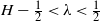 $H-\frac{1}{2}< \lambda < \frac{1}{2}$
and
 $\smash{k^* =\xi(\text{e}^{\frac{1}{1-2\lambda}}_1)}$
, which in turn implies
 $e(k^*,T) = \lceil d \varepsilon^{-2}_{k^*} T\rceil$
number of steps in the algorithm. The underlying state
 $\smash{\mathcal{A}^{k^*}_{e(k^*,T)}}$
lives in an
 $e(k^*,T)(d +1)$
-dimensional space. A concrete Monte Carlo scheme is developed in the companion paper by Bezerra et al. [Reference Bezerra, Ohashi, Russo and Souza7]. Lastly, we mention that there is no conceptual obstruction to computing sensitivities of S w.r.t. B (hedging strategies) by projecting the optimization problem onto the filtration
 $$
{({\cal F}_t^k)_{0 \le t \le T}}
$$
and working with the differential operators introduced in [Reference Leão, Ohashi and Simas27] which describe Doob–Meyer decompositions for test processes. This will be investigated in a future project.
This paper is organized as follows. In Section 2 we present the basic objects of our discretization scheme. In Section 3, we present the main results of the paper and we explain how the methodology can be concretely used to solve optimal stopping problems beyond the Markovian case. In Section 4 we present the proofs of Proposition 1 and Theorem 1. Section 5 illustrates the methodology with two examples. Section 5.3 explains how to operationalize the discrete-time dynamic programming principle in a concrete example.
2. Preliminaries
Throughout this article we are going to fix a d-dimensional Brownian motion
 $B = \{B^{1},\ldots,B^{d}\}$
on the usual stochastic basis
 $(\Omega, \mathbb{F}, \mathbb{P})$
, where
 $\Omega$
is the space
 $$
C([0,+\infty);\mathbb{R}^d) := \{f:[0,+\infty) \rightarrow
\mathbb{R}^d~\text{continuous}\}
$$
, equipped with the usual topology of uniform convergence on compact intervals.
 $\mathbb{P}$
is the Wiener measure on
 $\Omega$
such that
 $\mathbb{P}\{B(0) = 0\}=1 $
and
 $\mathbb{F}:=(\mathcal{F}_t)_{t\ge 0}$
is the usual
 $\mathbb{P}$
-augmentation of the natural filtration generated by the Brownian motion. In the following we recall the basic structure of the theory presented by [Reference Leão and Ohashi26, Reference Leão, Ohashi and Simas27], and we refer the reader to these works for all unexplained points.
For a fixed positive sequence
 $\{\varepsilon_k;\,\,k\ge 1\}$
such that
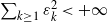 $\sum_{k\ge 1}\varepsilon^2_k< +\infty$
, and for each
 $j = 1, \ldots, d$
, we define
 $T^{k,j}_0 := 0$
almost surely (a.s.) and we set
 \begin{equation}
T^{k,j}_n := \inf\big\{T^{k,j}_{n-1}< t <\infty; |B^{j}(t) - B^{j}(T^{k,j}_{n-1})| = \epsilon_k\big\}, \quad n \ge 1.
\label{eqn4}
\end{equation}
For each
 $j\in \{1,\ldots,d \}$
, the family
 $
(T^{k,j}_n)_{n\ge 0}
$
is a sequence of
 $\mathbb{F}$
stopping times and the strong Markov property implies that the increments
 $\smash{\{T^{k,j}_n - T^{k,j}_{n-1};\,\,n\ge 1\}}$
are an independent and identically distributed sequence with the same distribution as
 $\smash{T^{k,j}_1}$
. Moreover,
 $\smash{T^{k,j}_1}$
is an absolutely continuous variable (see [Reference Borodin and Salminen9, Reference Leão, Ohashi and Simas27]).
From this family of stopping times, we define
 $A^{k}:=(A^{k,1},\ldots, A^{k,d})$
as the d-dimensional step process whose components are given by
 A^{k,j} (t) :=
\sum_{n=1}^{\infty}\epsilon_k~\sigma^{k,j}_n{1}_{\{T^{k,j}_n\leq t
\}};~t\ge0,
where
 \sigma^{k,j}_n:=\left\{\!\!
\begin{array}{rl}
1 & \hbox{if} \ B^{\:j} (T^{k,j}_n) - B^{\:j} (T^{k,j}_{n-1}) > 0, \\[4pt]
-1 & \hbox{if} \ B^{\:j} (T^{k,j}_n) - B^{\:j} (T^{k,j}_{n-1})< 0, \\
\end{array}
\right.
for
 $k,n\ge 1$
and
 $j=1, \ldots , d$
. Let
 $\mathbb{F}^{k,j} := \{ \mathcal{F}^{k,j}_t;\ t\ge 0 \} $
be the natural filtration generated by
 $\{A^{k,j}(t);\ t \ge 0\}$
. The multidimensional filtration generated by
 $A^k$
is naturally characterized as follows. Let
 $\mathbb{F}^{k} := \{\mathcal{F}^{k}_t ;\ 0 \leq t <\infty\}$
be the product filtration given by
 $\mathcal{F}^{k}_t := \mathcal{F}^{k,1}_t \otimes\mathcal{F}^{k,2}_t\otimes\cdots\otimes\mathcal{F}^{k,d}_t$
for
 $t\ge 0$
. Let
 $\mathcal{T}:=\{T^{k}_m;\ k,m\ge 0\}$
be the order statistics obtained from the family of random variables
 $\{T^{k,j}_\ell;\,\,\ell,k\ge 0 ;\,\,j=1,\ldots,d\}$
. That is, we set
 $T^{k}_0:= 0$
,
 \begin{equation}
T^{k}_1:= \inf_{1\le \kern1ptj\le d}\{T^{k,j}_1 \},\quad T^{k}_n:= \inf_{\substack {1\le \kern1ptj\le d\\ m\ge 1} } \{T^{k,j}_m ;\ T^{k,j}_m \ge T^{k}_{n-1}\}
\label{eqn5}
\end{equation}
for
 $n\ge 1$
.
The structure
 ${\cal D} :=\{\mathcal{T}, A^{k,j};\ 1\le \kern1ptj\le d, k\ge 1\}$
is a discrete-type skeleton for the Brownian motion in the language of [Reference Leão, Ohashi and Simas27] (see their Definition 2.1). Throughout this article we set
 \begin{equation}
\Delta T^{k}_n:= T^{k}_n - T^{k}_{n-1},\quad N^{k}(t):= \max\{n;\,\,T^{k}_n\le t\},\quad \bar{t}_k:=\max\{T^k_n;\,\,T^k_n \le t\};\,\,t\ge 0,
\label{eqn6}
\end{equation}
and
 \eta^{k,j}_n:=\left\{\!\!\!
\begin{array}{rl}
1 & \hbox{if} \ \Delta A^{k,j} (T^k_n)>0, \\
-1 & \hbox{if} \ \Delta A^{k,j} (T^k_n)< 0, \\
0 & \hbox{if} \ \Delta A^{k,j} (T^k_n)=0,
\end{array}
\right.
for
 $n\ge 1$
. Let us denote
 $\eta^k_n:=(\eta^{k,1}_n, \dots, \eta^{k,d}_n)$
,
 \mathbb{I}_k:=\Big\{ (i^k_1, \ldots, i^k_d); i^k_\ell\in \{-1,0,1\}~\forall
\ell \in \{1,\ldots, d\}~\text{and}~\sum_{j=1}^d|i^k_j|=1 \Big\}
and
 $\mathbb{S}_k:=(0,+\infty)\times \mathbb{I}_k$
for
 $k,n\ge 1$
. The n-fold Cartesian product of
 $\mathbb{S}_k$
is denoted by
 $\mathbb{S}_k^n$
and a generic element of
 $\mathbb{S}^n_k$
will be denoted by
 $
{b}^k_n := (s^k_1,\tilde{i}^k_1, \ldots, s^k_n, \tilde{i}^k_n)\in
\mathbb{S}^n_k
$
where
 $
(s^k_r,\tilde{i}^k_r)\in (0,+\infty)\times
\mathbb{I}_k
$
for
 $1\le r\le n$
. We also denote
 t^k_j:=\sum_{\ell=1}^j s^k_\ell,
for a given list
 $
(s^k_1, \ldots, s^k_j)\in (0,+\infty)^j
$
where
 $j\ge 1$
. The driving noise in our methodology is given by the following discrete-time process:
 \label{Aknvariable}
\mathcal{A}^k_n:= (\Delta T^k_1, \eta^k_1, \ldots, \Delta T^k_n, \eta^k_n)\in \mathbb{S}^n_k~\text{a.s.}
One should notice that
 $\mathcal{F}^k_{T^k_n} = (\mathcal{A}^k_n)^{-1}(\mathcal{B}(\mathbb{S}^n_k))$
up to
 $\mathbb{P}$
-null sets, where
 $\mathcal{B}(\mathbb{S}^k_n)$
is the Borel
 $\sigma$
-algebra generated by
 $\mathbb{S}^n_k;\,\,n\ge 1$
.
2.1. Transition probabilities
The law of the system will evolve according to the following probability measure defined on
 $$\mathbb{P}^k_n(E):=\mathbb{P}\{\mathcal{A}^k_n\in E\};\,\,E\in \mathcal{B}(\mathbb{S}^n_k), n\ge 1.$$
By its definition,
 $\mathbb{P}^k_{n}(\!\cdot\!) = \mathbb{P}^k_{r}(\!\cdot\!\times \mathbb{S}^{r-n}_k)$
for any
 $r> n\ge 1$
. By construction,
 $\mathbb{P}^k_{r}(\mathbb{S}^{n}_k\times\!\cdot\!)$
is a regular measure and
 $\mathcal{B}(\mathbb{S}_k)$
is countably generated, so it is well known that there exists (
 $\smash{\mathbb{P}^k_{n}}$
-a.s. unique) a disintegration
 $\nu^k_{n,r}\,:\, \mathcal{B}(\mathbb{S}^{r-n}_k)\times\mathbb{S}^{n}_k\rightarrow[0,1]$
that realizes
 $$
_r^k(D) = \int_{_k^n} {\int_{_k^{r - n}} {{{\bf{1}}_D}} } (b_n^k,q_{n,r}^k)\nu _{n,r}^k({\mkern 1mu} {\rm{d}}q_{n,r}^k\mid b_n^k)_n^k({\mkern 1mu} {\rm{d}}b_n^k),$$
for every
 $D\in \mathcal{B}(\mathbb{S}^{r}_k)$
, where
 $q^k_{n,r}$
is the projection of
 $$
b_r^k
$$
onto the last
 $(r-n)$
components, i.e.
 $q^k_{n,r} = (s^k_{n+1},\tilde{i}^k_{n+1}, \ldots,s^k_{r},\tilde{i}^k_{r} )$
for a list
 $
{b}^k_r = (s^k_1,\tilde{i}^k_1, \ldots, s^k_r,\tilde{i}^k_r)\in \mathbb{S}^r_k
$
. We sometimes denote
 $\nu^k_{0,r}:=\mathbb{P}^k_r$
for
 $r\ge 1$
. If
 $r=n+1$
, we denote
 $\nu^k_{n+1}:=\nu^k_{n,n+1}$
. For an explicit formula for this conditional probability we refer the reader to [Reference Leão, Ohashi and Souza29].
Let
 $
{B}^p(\mathbb{F})
$
be the space of continuous from the left with right limits (càdlàg)
 $\mathbb{F}$
-adapted processes Y such that
 $$\|Y\|^p_{{\textbf{B}}^p}:=\mathrm{E}\| Y\|^p_{\infty} < \infty,$$
where
 $\|Y\|_\infty:=\sup_{0\le t\le T}|Y(t)|$
,
 $1\le p< \infty$
, and
 $0 < T < +\infty$
is a fixed terminal time. In the following,
 $[\!\cdot, \cdot\!]$
is the
 $\mathbb{F}^k$
-quadratic variation operator. The following class of
 $\mathbb{F}^k$
-adapted processes whose underlying differential structure and asymptotics were studied in [Reference Leão, Ohashi and Simas27] will play a key role in this work.
Definition 1. We say that
 $\mathcal{Y} = ((X^k)_{k\ge 1},{\cal D})$
is an imbedded discrete structure for
 $X\in {\textbf{B}}^p(\mathbb{F})$
if
 $X^k$
is a sequence of
 $\mathbb{F}^k$
-adapted pure jump processes of the form
 $$
X^k(t) = \sum_{n=0}^\infty X^{k}(T^k_n)\mathbf{1}_{\{T^k_n\le t < T^k_{n+1}\}};,\quad 0\le t\le T,
\label{eqn7}$$
that has integrable quadratic variation
 $\mathrm{E}[X^k,X^k](T)< \infty,\ k\ge 1$
, and
 $$\lim_{k\rightarrow+\infty}\|X^k-X\|_{{\textbf{B}}^p}=0
\label{eqn8}$$
for some
 $p\ge 1$
.
3. Construction of an imbedded structure for S and near-optimal stopping times
For
 $t\le T$
, we denote
 $\mathcal{T}_t(\mathbb{F})$
as the set of all
 $\mathbb{F}$
stopping times
 $\tau$
such that
 $t\le \tau\le T$
a.s. For
 $n\geq 0$
, we denote
 $\mathcal{T}_{k,n}(\mathbb{F}):=\mathcal{T}_{t}(\mathbb{F})$
for
 $t=T^k_n$
. To shorten the notation, we set
 $\mathcal{T}_{k,n}:=\mathcal{T}_{k,n}(\mathbb{F})$
. Throughout this article we assume that the reward process Z is an
 $\mathbb{F}$
-adapted continuous process that satisfies the integrability regularity condition
 $$|Z|^p_{{\textbf{B}}^p}< \infty\ ~\forall
\text{for all}\ p\ge 1.\tag*{(A1)}$$
For a given reward process Z, let S be the Snell envelope associated with Z:
 $$S (t):= \text{ess} \sup_{\tau\in \mathcal{T}_t(\mathbb{F})} \mathbb{E} \left[ Z(\tau) \mid \mathcal{F}_t \right], \quad 0 \leq t \leq T.$$
We assume that S satisfies the following integrability condition:
 $$|S|^p_{{\textbf{B}}^p}< \infty\ ~\forall
\text{for all}\ p\ge 1.\tag*{(A2)}$$
Assumptions (A1) and (A2) are not essential in the sense that the range of integrability can be relaxed. In order to simplify the exposition, we then assume that (A1) and (A2) hold true. Since the optimal stopping time problem at hand takes place on the compact set [0,T], it is crucial to know the correct number of periods in our discretization scheme. For this purpose, let
 $\lceil x\rceil$
be the smallest natural number greater than or equal to
 $x\ge 0$
. We then denote
 $$e(k,T):= d\lceil \varepsilon^{-2}_k T\rceil,;
\quad k\ge 1.$$
Lemma 1. For any 0 < T < ∞,
 $$\mathbb{E}|T^{k}_{e(k,T)}- T|^2 \rightarrow 0$$
and
 $T^k_{e(k,T)}\rightarrow T$
a.s. as
 $k\rightarrow \infty$
.
Proof. Just notice that
 $$|T^k_{d\lceil \varepsilon_k^{-2}T \rceil} - T|\le \max\Big\{|\max_{1\le i\le d} T^{k,i}_{\lceil \varepsilon_k^{-2}T \rceil} - T|, \, |\min_{1\le i\le d}T^{k,i}_{\lceil \varepsilon_k^{-2}T \rceil} - T| \Big\}~a.s.$$
for every
 $k\ge 1$
. We then apply Lemma 2.2 in [Reference Khoshnevisan and Lewis24] to conclude the proof.
Due to this result we will reduce the analysis to the deterministic number of periods e(k,T). We denote
 $D^{k,m}_n$
as the set of all
 $\mathbb{F}^k$
stopping times of the form
 $$\tau = \sum_{i=n}^{m}T^k_i\mathbf{1}_{\{\tau = T^k_i\}},$$
where
 $\smash{\{\tau = T^k_i;\,\,i=n, \ldots, m\}}$
is a partition of
 $\Omega$
and
 $0\le n \le m$
. Let us denote
 $\smash{D^k_{n,T} :=}$
 $\smash{\{\eta\wedge T;\,\,\eta\in D^{k,\infty}_n\}}$
. We observe that
 $D^{k,\infty}_0$
is the set of all
 $\mathbb{F}^k$
totally inaccessible stopping times.
Let
 $\{Z^k;\,\,k\ge 1\}$
be a sequence of pure jump processes of the form (7) and let
 $\{S^k;\,\,k\ge 1\}$
be the associated value process given by
 $$S^k(t) := \sum_{n=0}^{\infty} S^k(T^k_n)\mathbf{1}_{\{T^k_n\le t \wedge T^k_{e(k,T)}< T^k_{n+1}\}},;
\quad 0\le t\le T,
\label{eqn9}$$
where for
 $0\le n\le e(k,T)$
we denote
 $${S^k}(T_n^k): = {\rm{ }}\mathop {{\rm{ess sup}}}\limits_{_{\tau \in D_n^{k,e(k,T)}}} [{Z^k}(\tau \wedge T)|{\cal F}_{T_n^k}^k]\quad {\rm{and}}\quad {U^{{\cal Y},k,p}}S(T_n^k): = [{{\Delta {S^k}(T_{n + 1}^k)} \over {_k^2}}|{\cal F}_{T_n^k}^k].$$
The following result shows the fundamental role played by the imbedded discrete structure driven by a skeleton
 ${\cal D} :=\{\mathcal{T}, A^{k,j};\,\,1\le \kern1ptj\le d,\ k\ge 1\}$
: it enables lifting the discrete structure into the Brownian filtration without losing
 $\mathbb{F}^k$
-adaptedness in the optimization problem. We postpone the proof of Proposition 1 to Section 4.
Proposition 1. Let Zk be a pure jump process of the form (7). For each n ≥ 0 and k ≥ 1, we have
 $$\mathop {{\rm{ess sup}}}\limits_{_{\tau \in D_{n,T}^k}} [{Z^k}(\tau )|{\cal F}_{T_n^k}^k] = {\rm{ }}\mathop {{\rm{ess sup}}}\limits_{_{\tau \in {{\cal T}_{k,n}}}} [{Z^k}(\tau )|{\cal F}_{T_n^k}^k]a.s.$$
3.1.
 $\varepsilon$
-optimal stopping times

The dynamic programming algorithm allows us to define the stopping and continuation regions as follows:
 $$\begin{align*}
{\textbf{{S}}}(i,k) & :=\{{\textbf{B}}^k_{i}\in \mathbb{S}^{i}_k;\,\,\mathbb{Z}^k_i({\textbf{B}}^k_i) = \mathbb{V}^k_i({\textbf{B}}^k_i) \}\quad \text{(stopping region)} \\
{\textbf{{D}}}(i,k) & :=\{{\textbf{B}}^k_{i}\in \mathbb{S}^{i}_k;\,\,\mathbb{V}^k_i({\textbf{B}}^k_i) > \mathbb{Z}^k_i({\textbf{B}}^k_i) \}\quad \text{(continuation region)}
\end{align*}
$$
where
 $0\le i\le e(k,T)$
, and
 $\mathbb{V}^k_n\,:\,\mathbb{S}^n_k\rightarrow\mathbb{R}$
and
 $\mathbb{Z}^k_n\,:\,\mathbb{S}^n_k\rightarrow\mathbb{R}$
are Borel functions that realize
 $$
S^{k}(T^k_n) = \mathbb{V}^k_n(\mathcal{A}^k_n)~\text{a.s.}\ \quad
\text{and}~Z^k(T^k_n\wedge T) = \mathbb{Z}^k_n(\mathcal{A}^k_n)~\text{a.s.},;
\quad n=0, \ldots, e(k,T).
\label{eqn10}$$
Let
 $Y^k(i):= Z^k(T^k_i\wedge T);\,\,i\ge 0$
. We set
 $J^{k,m}_n$
as the set of all
 $(\mathcal{F}^k_{T^k_i})^m_{i=0}$
stopping times taking values on
 $\{n,n+1, \ldots, m\}$
for a given
 $0\le n < m < \infty$
. Following the classical theory of discrete optimal stopping, the smallest
 $$({\cal F}_{T_i^k}^k)_{i = 0}^{e(k,T)}$$
-optimal stopping time w.r.t. the problem
 $$\sup_{\tau \in J^{e(k,T)}_0}\mathbb{E} \big[Y^k(\tau)\big]$$
is given by
 $$\begin{align}
\tau^{k} & := \min \{0\le \kern1ptj\le e(k,T);\,\, \mathcal{A}^k_{j}\in {\textbf{{S}}}(\kern1.5ptj,k)\} \nonumber \\
& \;= \min\{0\le \kern1ptj\le e(k,T);\,\,S^{k}(T^k_j) = Z^k(T^k_j \wedge T)\},
\label{eqn11}\end{align}
$$
which is finite a.s. by construction. Moreover,
 $$
\text{ess}~
\esssup_{\eta\in J^{k,e(k,T)}_n}\mathrm{E}[Y^k(\eta) \!\mid\! \mathcal{F}^{k}_{T^k_n}]=\!\esssup_{\tau\in D^{k,e(k,T)}_n}\mathrm{E}[Z^k(\tau\wedge T) \!\mid\! \mathcal{F}^{k}_{T^k_n}]~\text{a.s.}
\label{eqn12}$$
for each
 $0\le n \le e(k,T)$
. The dynamic programming principle can be written as
 $$
\left\{\!\!\begin{array}{ll}
\tau^{k}_{e(k,T)} & := e(k,T) , \\
\tau^{k}_{j} & := j \mathbf{1}_{G^k_j} + \tau^{k}_{j+1}\mathbf{1}_{(G^{k}_j)^c},\quad 0\le \kern1ptj \le e(k,T)-1,
\end{array}\right.
\label{eqn13}
$$
where
 G^k_j:= \{\mathbb{Z}^k_j (\mathcal{A}^k_j)\ge \mathrm{E}[\mathbb{Z}^k_{\tau^{k}_{j+1}}(\mathcal{A}^k_{\tau^{k}_{j+1}}) \,|\, \mathcal{A}^k_j]\}, \quad 0\le \kern1ptj\le e(k,T)-1,$$
and
 $\tau^{k}=\tau^{k}_0$
a.s. The sequence of functions
 ${\textbf{{U}}}^k_j\,:\,\mathbb{S}^j_k\rightarrow\mathbb{R}$
,
 $$
{\textbf{B}}^k_j\mapsto {\textbf{{U}}}^k_j({\textbf{B}}^k_j):=\mathrm{E}[\mathbb{Z}^k_{\tau^{k}_{j+1}}(\mathcal{A}^k_{\tau^{k}_{j+1}}) \,|\, \mathcal{A}^k_j={\textbf{B}}^k_j],\quad 0\le \kern1ptj\le e(k,T)-1 ,
\label{eqn14}
$$
are called continuation values and they play a key role in the obtention of the optimal value.
The value functional which gives the best payoff can be reconstructed by means of the dynamic programming principle over the e(k,T) steps which provides
 $$\sup_{\eta\in J^{k,e(k,T)}_0}\mathrm{E}[Y^k(\eta)] =\max\{\mathbb{Z}^k_0(\textbf{0});\,\,\mathrm{E}[\mathbb{V}^k_1 (\mathcal{A}^k_1)]\},$$
where
 $\mathrm{E}[\mathbb{V}^k_1 (\mathcal{A}^k_1)] = \mathrm{E}[\mathbb{Z}^k_{\tau^{k}_1}(\mathcal{A}^k_{\tau^{k}_1})]$
. Moreover,
 $$
\mathrm{E}[Y^k(\tau^k)]=\mathrm{E}[Z^k(T^k_{\tau^{k}}\wedge T)] = \sup_{\tau\in D^k_{0,T}} \mathrm{E}[Z^k(\tau \wedge T^k_{e(k,T)})]=\sup_{\tau\in \mathcal{T}_{0}(\mathbb{F})}\mathrm{E} [Z^k(\tau \wedge T^k_{e(k,T)})],
\label{eqn15}
$$
where the last fundamental equality in identity (15) is due to Proposition 1. Let us denote
 $$
V^k_0:= \sup_{\tau\in D^k_{0,T}}\mathrm{E}[Z^k(\tau\wedge T^k_{e(k,T)})],;
\quad k\ge 1.
\label{eqn16}
$$
We are now able to state the main results of this article. The proof of Theorem 1 is postponed to Section 4.
Theorem 1. Let S be the Snell envelope associated to a reward process Z satisfying assumptions (A1) and (A2). Let
 $\{Z^k;\,\,k\ge 1\}$
be a sequence of pure jump processes of the form (7) and let
 $\{S^k;\,\,k\ge 1\}$
be the associated value process given by (9). If
 $\mathcal{Z} = ( (Z^k)_{k\ge 1},{\cal D})$
is an imbedded discrete structure for Z where (8) holds for
 $p>1$
, then
 $\mathcal{S} =
((S^k)_{k\ge 1},{\cal D})$
is an imbedded discrete structure for S, where
 \lim_{k\rightarrow+\infty}\mathrm{E}\sup_{0\le t\le T}|S^k(t) - S(t)|=0.$$
Moreover,
 $ \{S^k;\,\,k\ge 1\}$
is the unique sequence of pure jump processes of the form (7) which satisfies the following variational inequality:
 $$\begin{align}
\max \{ U^{\mathcal{Y},k,{\textbf{{p}}}}S(T^k_i);\,\, Z^k(T^k_i\wedge T) - S^{k}(T^k_i) \} & = 0,\quad i=e(k,T)-1, \ldots, 0,~a.s. \label{eqn17}\end{align}
$$
 $$\begin{align}
\nonumber S^{k} (T^k_{e(k,T)}) & = Z^k (T^k_{e(k,T)}\wedge T)~a.s.
\end{align}
$$
Theorem 2. Let
 $\mathcal{Z} = ((Z^k)_{k\ge 1},{\cal D})$
be an imbedded discrete structure for the reward process Z and let
 $\tau^k$
be the optimal stopping time given by (11). Then
 $T^k_{\tau^{k}}\wedge T$
is an
 $\varepsilon$
-optimal stopping time in the Brownian filtration, i.e. for a given
 $\varepsilon>0$
,
 \sup_{\eta\in \mathcal{T}_0(\mathbb{F})}\mathrm{E}[Z(\eta)] -\varepsilon< \mathrm{E}[Z(T^k_{\tau^k}\wedge T)]$$
for every k sufficiently large. Moreover,
 $$
\big|\sup_{\tau\in \mathcal{T}_0(\mathbb{F})}\mathrm{E}[Z(\tau)] - V^k_0\big|\le \mathrm{E}\|Z^k(\!\cdot\!\wedge T^k_{e(k,T)}) - Z\|_\infty\rightarrow 0
\label{eqn18}
$$
as
 $k\rightarrow+\infty$
.
Proof. The imbedded discrete structure property, the path continuity of Z, and Lemma 1 yield
 $$\mathrm{E}\| Z^k(\!\cdot\!\wedge T^k_{e(k,T)}) - Z\|_\infty\rightarrow 0$$
as
 $k\rightarrow +\infty$
. This shows that
 $$\begin{equation}
|\sup_{\tau\in \mathcal{T}_0(\mathbb{F})}\mathrm{E}[Z^k(\tau \wedge T^k_{e(k,T)})] - \sup_{\tau\in \mathcal{T}_0(\mathbb{F})} \mathrm{E}[Z(\tau)]|\le\mathrm{E}\sup_{0\le t\le T}|Z^k(t\wedge T^k_{e(k,T)}) - Z(t)|\rightarrow 0
\label{eqn19}
\end{equation}
$$
as
 $k\rightarrow +\infty$
. By (15) (see also Proposition 1), (16), and (12), we conclude (18). Now, by using (15) and (19), for a given
 $\varepsilon>0$
we have
 $$\begin{equation}
\sup_{\tau\in \mathcal{T}_0(\mathbb{F})}\mathrm{E}[Z(\tau)] - \varepsilon< \sup_{\tau\in \mathcal{T}_0(\mathbb{F})} \mathrm{E}[Z^k(\tau \wedge T^k_{e(k,T)} \wedge T)] = \mathrm{E}[Z^k(T^k_{\tau^{k}}\wedge T)]
\label{eqn20}
\end{equation}
$$
for every k sufficiently large. The imbedded discrete structure property of
 $Z^k$
yields
 $\mathrm{E}[Z^k(T^k_{\tau^{k}}\wedge T)] <\mathrm{E}[Z(T^k_{\tau^{k}}\wedge T)] + \varepsilon $
for every k sufficiently large. This implies that
 $\sup_{\tau\in\mathcal{T}_0(\mathbb{F})}\mathrm{E}[Z(\tau)] - 2\varepsilon < \mathrm{E}[Z(T^k_{\tau^{k}}\wedge T)]$
for every k sufficiently large. It remains to show that
 $T^k_{\tau^k}$
is an
 $\mathbb{F}$
stopping time. Clearly,
 $T^k_{\tau^k}\,:\,\Omega\rightarrow \mathbb{R}_+$
is
 $\mathcal{F}$
-measurable. We claim that
 T^k_{\tau^k(\omega)}(\omega)\le t~\text{and}~\omega|_{[0,t]} = \omega'|_{[0,t]} %~\text{then}~
\implies T^k_{\tau^k(\omega)}(\omega) = T^k_{\tau^k(\omega')}(\omega').$$
Recall that
 $\tau^{k}(\omega)=\min \{0\le \kern1ptj\le e(k,T);\,\,\mathcal{A}^k_{j}(\omega)\in {\textbf{{S}}}(\kern1.5ptj,k)\}$
, and we notice that
 $\smash{T^k_{\tau^k(\omega)}(\omega)\le t}$
means that all the information that we need to compute
 $\smash{T^k_{\tau^k(\omega)}(\omega)}$
lies on the Brownian path
 $\omega|_{[0,t]}$
. This can be easily seen by the fact that each continuous-time random walk
 $A^{k,j};\,\,j=1, \ldots, d$
only (possibly) jumps at the stopping times
 $(T^k_n)_{n\ge 0}$
. In this case, if
 $\omega|_{[0,t]} = \omega'|_{[0,t]}$
and
 $T^k_{\tau^k(\omega)}(\omega)\le t$
, then we necessarily have
 $T^k_{\tau^k(\omega)}(\omega) = T^k_{\tau^k(\omega')}(\omega')$
. From Galmarino’s test (see [Reference Dellacherie and Meyer16] Nos. IV 94–103, pp. 145–152), we conclude that
 $T^k_{\tau^k}$
is an
 $(\widetilde{\mathcal{F}}_t)_{t\ge 0}$
stopping time, where
 $(\widetilde{\mathcal{F}}_t)_{t\ge 0}$
is the raw filtration generated by the Brownian motion on the Wiener space. This shows that
 $T^k_{\tau^k}\wedge T$
is an
 $\mathbb{F}$
stopping time and (20) allows us to conclude the proof.
Remark 1. The importance of imbedded discrete structures is already apparent in Theorem 2: Maximization along the discrete type filtration
 $(\mathcal{F}^k_{T^k_n})_{n=0}^{e(k,T)}$
is essentially equivalent to maximization along the Brownian filtration for k large enough. More importantly, the imbedded structure allows us to reduce the dimensionality of the optimal stopping problem (see Section 5.3 and Example 1).
4. Proofs of Proposition 1 and Theorem 1
In order to prove convergence, we need a subtle pathwise argument on the conditional expectations involved in the optimization problem. For a given pure jump process of the form (7), there exists a list of Borel functions
 $h^k_\ell\,:\,\mathbb{S}_k^\ell\rightarrow \mathbb{R}$
which realizes
 Z^k(t) = \sum_{\ell=0}^{\infty} h^k_\ell(\mathcal{A}^k_\ell)\mathbf{1}_{\{T^k_\ell \le t < T^k_{\ell+1}\}}~\text{a.s.},;
\quad 0\le t\le T.$$
In other words,
 $\mathbb{Z}^k_n(\mathcal{A}^k_n) = Z^k(T^k_n\wedge T)$
a.s., where
 $$\mathbb{Z}^k_n({\textbf{B}}^k_n)=\left\{\!\!
\begin{array}{rl}
h^k_n({\textbf{B}}^k_n) & \hbox{if} \ t^k_n\le T , \\
h^k_j({\textbf{B}}^k_j) & \hbox{if} \ T < t^k_n,\ t^k_j\le T < t^k_{j+1} \\
\end{array}
\right.$$
for
 $n\ge 0$
. In the following we fix two natural numbers
 $0\le n \le r$
. For a given
 $\tau\in D^{k,r}_n$
, there exists a list of Borel functions
 $g^k_\ell\,:\,\mathbb{S}_k^\ell\rightarrow \mathbb{R}$
that realizes
 $$\begin{equation}
\tau = \sum_{\ell=n}^r T^k_\ell g^k_\ell(\mathcal{A}^k_\ell)~\text{a.s.},
\label{eqn21}
\end{equation}
$$
where
 $g^k_\ell(\mathcal{A}^k_\ell) = \mathbf{1}_{\{\tau = T^k_\ell\}},\ n\le \ell \le r$
. The action space in our optimization problem is given by
 \mathbb{A}^j := \bigg\{x = (x_1,\ldots, x_j)\in \mathbb{N}^j;\,\,\sum_{\ell=1}^j x_\ell = 1\bigg\}, \quad j>1.$$
The elements of
 $\mathbb{A}^{r-n+1}\times \mathbb{S}^r_k$
will be denoted by
 {\textbf{{o}}}^{k,n,r}:=(a^k_n, \ldots, a^k_r, {\textbf{B}}^k_r).$$
For a given list of Borel functions
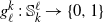 $g^k_\ell\,:\,\mathbb{S}_k^\ell\rightarrow \{0,1\}$
realizing (21), we define the map
 $\smash{\Xi^{k,g^k}_{n,r}\,:\,\mathbb{S}^r_k\rightarrow \mathbb{A}^{r-n +1}\times \mathbb{S}^r_k}$
given by
 \Xi^{k,g^k}_{n,r}({\textbf{B}}^k_r):= ( g^k_n({\textbf{B}}^k_n), \ldots, g^k_r({\textbf{B}}^k_r), {\textbf{B}}^k_r), %;~
\quad {\textbf{B}}^k_r\in \mathbb{S}^r_k.$$
We observe that we may choose
 $(g^k_\ell)_{\ell=n}^r$
in such a way that
 $(g^k_n({\textbf{B}}^k_n), \ldots, g^k_r({\textbf{B}}^k_r))\in\mathbb{A}^{r-n+1}$
for every
 ${\textbf{B}}^k_r\in \mathbb{S}^r_k$
. Moreover, there exists an explicit map
 $\gamma^k_{n,r}\,:\,\mathbb{A}^{r-n+1}\times \mathbb{S}^r_k\rightarrow\mathbb{R}$
such that
 $$\begin{equation}
Z^k(\tau \wedge T) = \gamma^k_{n,r}( \Xi^{k,g^k}_{n,r}(\mathcal{A}^k_r))~\text{a.s.},
\label{eqn22}
\end{equation}
$$
where
 $$\begin{align*}
\gamma^k_{n,r}({\textbf{{o}}}^{k,n,r}) & := \sum_{\ell=n}^r h^k_\ell({\textbf{B}}^k_\ell)\mathbf{1}_{\{1\}}(a^k_\ell)\mathbf{1}_{\{t^k_\ell \le T\}}({\textbf{B}}^k_\ell) \\
& \quad +\sum_{\ell=n}^r h^k_\ell({\textbf{B}}^k_\ell)\mathbf{1}_{\{t^k_\ell\le T < t^k_{\ell+1}\}}\bigg(\sum_{j=n}^r\mathbf{1}_{\{1\}}(a^k_j)\mathbf{1}_{\{t^k_j > T\}}({\textbf{B}}^k_j)\bigg).
\end{align*}
$$
We should also compute a pathwise representation of
 $Z^k(\tau\wedge T)$
but for a slightly more general class of stopping times. Let
 $\widetilde{\mathcal{T}}_{k,n,r}$
be the set of all
 $\mathbb{F}$
stopping times of the form
 \eta = \sum_{\ell=n}^r T^k_{\ell}\mathbf{1}_{\{\eta = T^k_\ell\}} ,$$
where
 $\smash{\{\eta = T^k_\ell\}\in \mathcal{F}_{T^k_\ell};\,\,n\le \ell\le r}$
. Of course,
 $D^{k,r}_n\subset \widetilde{\mathcal{T}}_{k,n,r}$
for every
 $0\le n \le r $
and
 $k\ge 1$
. Recall that
 $T^k_n < \infty$
a.s. for every
 $n\ge 0$
. In this case, it is known (see, e.g., Corollary 3.22 in [Reference He, Wang and Yan22]) that
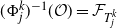 $(\Phi^k_j)^{-1}(\mathcal{O}) = \mathcal{F}_{T^k_j}$
, where
 $\mathcal{O}$
is the optional
 $\sigma$
-algebra on
 $\Omega\times \mathbb{R}_+$
and
 \Phi^k_j(\omega):= (\omega, T^k_j(\omega)),;
\quad \omega\in \Omega^*,~j\ge 1,$$
where
 $\mathbb{P}(\Omega^*)=1$
. To keep the notation simple we choose a version of
 $\Phi^k_j$
defined everywhere, and with a slight abuse of notation we write it as
 $\smash{\Phi^k_j}$
. Based on this fact, for a given
 $\smash{\eta\in\widetilde{\mathcal{T}}_{k,n,r}}$
there exists a list of Borel functions
 $\varphi^k_\ell\,:\,\Omega\times\mathbb{R}_+\rightarrow \{0,1\}$
that realizes
 $$\begin{equation}
\eta = \sum_{\ell=n}^r T^k_\ell \varphi^k_\ell (\Phi^k_\ell)~\text{a.s.}
\label{eqn23}
\end{equation}
$$
For a list of Borel functions
 $\varphi^k_\ell\,:\,\Omega\times\mathbb{R}_+\rightarrow\{0,1\}$
realizing (23), we then define the map
 $\Xi^{k,\varphi^k}_{n,r}\,:\,\Omega\times \mathbb{R}^{r-n+1}_+\rightarrow\mathbb{A}^{r-n+1}\times \mathbb{S}^r_k$
given by
 \Xi^{k,\varphi^k}_{n,r}(\omega, x_n, \ldots, x_r,{\textbf{B}}^k_r):= ( \varphi^k_n(\Phi^k_n(\omega,x_n)), \ldots, \varphi^k_r(\Phi^k_r(\omega,x_r)), {\textbf{B}}^k_r)$$
for
 $\omega\in \Omega, (x_n, \ldots, x_r)\in \mathbb{R}^{r-n+1}_+$
and
 ${\textbf{B}}^k_r\in \mathbb{S}^r_k$
. By construction, we have
 $$\begin{equation}
Z^k(\eta\wedge T) = \gamma^k_{n,r}(\Xi^{k,\varphi^k}_{n,r}( J^k_{n,r}))~\text{a.s.},
\label{eqn24}
\end{equation}
$$
where
 $J^k_{n,r}:=(\text{Id}, T^k_n, \ldots, T^k_r, \mathcal{A}^k_r)$
and
 $\text{Id}\,:\,\Omega\rightarrow\Omega$
is the identity map.
In the following,
 $H^k_{n,r}\,:\,\mathcal{B}(\Omega\times \mathbb{R}^{r-n+1}_{+})\times\mathbb{S}^r_k\rightarrow[0,1]$
is the disintegration of
 $\mathbb{P}\circ J^k_{n,r}$
w.r.t
 $\mathbb{P}^k_r$
and
 $\nu^k_{n,r}$
is the disintegration of
 $\mathbb{P}^k_r$
w.r.t.
 $\mathbb{P}^k_n$
for
 $r > n\ge 1$
. Recall the notation introduced in Section 2.
Lemma 2. Let
 $Z^k$
be a pure jump process of the form (7). For each
 $\tau\in D^{k,r}_n$
and
 $\eta\in \widetilde{\mathcal{T}}_{k,n,r}$
, for
 $0\le n < r$
, we have
 $$\mathrm{E}[Z^k(\tau \wedge T)|\mathcal{F}^k_{T^k_n}] =\int_{\mathbb{S}^j_k}\gamma^k_{n,r}(\Xi^{k,g^k}_{n,r}(\mathcal{A}^k_n, q^k_{n,r}))\nu^k_{n,r}(\!\,{\rm d} q^k_{n,r} \!\mid\! \mathcal{A}^k_n)~\text{a.s.}$$
and
 $$\begin{multline*}
\mathrm{E}[Z^k(\eta \wedge T) \!\mid\! \mathcal{F}^k_{T^k_n}] =\int_{\mathbb{S}^j_k}\int_{\Omega\times \mathbb{R}^j_{+}}\gamma^k_{n,r}(\Xi^{k,\varphi^k}_{n,r}(\omega,x_n,\ldots,x_r,\mathcal{A}^k_n, q^k_{n,r}))H^k_{n,r} \\ (\!\,{\rm d}\omega \,{\rm d} x_n\ldots \,{\rm d} x_r \!\mid\! \mathcal{A}^k_n, q^k_{n,r})\nu^k_{n,r}(\!\,{\rm d} q^k_{n,r} \!\mid\! \mathcal{A}^k_n)
\end{multline*}
$$
a.s. for
 $j=r-n$
, where
 $(g^k_\ell)_{\ell=n}^r$
and
 $(\varphi^k_\ell)_{\ell=n}^r$
are Borel functions associated with
 $\tau$
and
 $\eta$
, respectively.
Proof. The proof is a direct consequence of the representations in (22) and (24), so we omit the details.
We are now able to prove Proposition 1, which is the main ingredient in the proof of Theorem 1 and the estimate (18) in Theorem 2.
Proof of Proposition 1. For the moment, let us fix
 $r > n$
. We claim that
 $$\begin{equation}
\esssup_{\tau\in \widetilde{\mathcal{T}}_{k,n,r} }\mathrm{E}[Z^k(\tau\wedge T) \!\mid\! \mathcal{F}^k_{T^k_n}] = \esssup_{\tau\in \overline{\mathcal{T}}_{k,n,r}}\mathrm{E}[Z^k(\tau\wedge T) \!\mid\! \mathcal{F}^k_{T^k_n}]~\text{a.s.},
\label{eqn25}
\end{equation}
$$
where
 $\overline{\mathcal{T}}_{k,n,r}:=\{\tau~\text{is an}~\mathbb{F}~\text{stopping time};~T^k_n\le \tau \le T^k_r~\text{a.s.}\}$
. For a given
 $\tau\in \overline{\mathcal{T}}_{k,n,r}$
, let us define the
 $\mathbb{F}$
stopping time
 $Q(\tau) = \min\{T^k_p;\,\, T^k_p > \tau\}$
and
 \eta(\tau) = \sum_{\ell=n}^{r+1}T^k_{\ell-1}\mathbf{1}_{\{Q(\tau) = T^k_\ell\}}\in \widetilde{\mathcal{T}}_{k,n,r}.$$
We observe that
 $\mathbb{P}\{\eta(\tau) = T^k_{n-1}\}=0$
. Moreover, since
 $Z^k$
has càdlàg paths, we have
 $$Z^k(\tau \wedge T) =Z^k((Q(\tau)\wedge T) -)=Z^k(\eta(\tau)\wedge T)~\text{a.s.}$$
This proves (25). We now claim that
 $$\begin{equation}
\esssup_{\tau\in \widetilde{\mathcal{T}}_{k,n,r} }\mathrm{E}[Z^k(\tau\wedge T) \!\mid\! \mathcal{F}^k_{T^k_n}] = \esssup_{\tau\in D^{k,r}_{n}}\mathrm{E}[Z^k(\tau\wedge T) \!\mid\! \mathcal{F}^k_{T^k_n}]~\text{a.s.}
\label{eqn26}
\end{equation}
$$
In order to check (26), we make use of Lemma 2 as follows. Let us define the following objects:
 F^k_{n,r}({\textbf{B}}^k_n):=\max_{(a^k_n,\ldots,a^k_r)\in \mathbb{A}^{r-n+1}}G^k_{n,r}(a^k_n,\ldots,a^k_r,{\textbf{B}}^k_n),$$
where
 G^{k}_{n,r}(a^k_n,\ldots,a^k_r, {\textbf{B}}^k_n):=\int_{\mathbb{S}^{r-n}_k}\gamma^k_{n,r}(a^k_n,\ldots,a^k_r,{\textbf{B}}^k_n, q^k_{n,r})\nu^k_{n,r}(\!\,{\rm d} q^k_{n,r} \!\mid\! {\textbf{B}}^k_n)$$
and
 \widetilde{F}^k_{n,r}({\textbf{B}}^k_n):=\max_{(a^k_n,\ldots,a^k_r)\in \mathbb{A}^{r-n+1}}\widetilde{G}^k_{n,r}(a^k_n,\ldots,a^k_r, {\textbf{B}}^k_n),$$
with
 $$\begin{multline*}
\widetilde{G}^k_{n,r}(a^k_n,\ldots,a^k_r, {\textbf{B}}^k_n)
:=\int_{\mathbb{S}^{r-n}_k}\int_{\Omega\times \mathbb{R}^{r-n+1}_{+}}\gamma^k_{n,r}(a^k_n,\ldots,a^k_r,{\textbf{B}}^k_n, q^k_{n,r}) \\
H^k_{n,r}(\!\,{\rm d}\omega \,{\rm d} x_n\ldots \,{\rm d} x_r \!\mid\! {\textbf{B}}^k_n, q^k_{n,r})\nu^k_{n,r}(\!\,{\rm d} q^k_{n,r} \!\mid\! {\textbf{B}}^k_n)
\end{multline*}
$$
for each
 ${\textbf{B}}^k_n\in \mathbb{S}^k_n$
and
 $(a^k_n,\ldots,a^k_r)\in \mathbb{A}^{r-n+1}$
. Since, for each
 $E\in \mathcal{B}(\mathbb{S}^{r-n}_k))$
and
 $F\in\mathcal{B}(\Omega\times \mathbb{S}^{r-n+1}_k)$
, the disintegrations
 {\textbf{B}}^k_n\mapsto \nu^k_{n,r}(E \!\mid\! {\textbf{B}}^k_n)~\text{and}~ {\textbf{B}}^k_r\mapsto H^k_{n,r}(F \!\mid\! {\textbf{B}}^k_r)$$
are Borel functions, then we can safely state (see Prop 7.29 in [Reference Bertsekas and Shreve6]) that both
 $G^k_{n,r}$
and
 $\widetilde{G}^k_{n,r}$
are Borel functions. Therefore, Lemma 2 yields
 $$\begin{align*}
G^{k}_{n,r}(\text{Pr}_n\circ\Xi^{k,g^k}_{n,r}(\mathcal{A}^k_n)) & = \mathrm{E}[Z^k(\tau\wedge T) \!\mid\! \mathcal{F}^k_{T^k_n}], \\ %\quad
\widetilde{G}^k_{n,r}(\text{Pr}_n\circ\Xi^{k,\varphi^k}_{n,r}(\mathcal{A}^k_n)) & = \mathrm{E}[Z^k(\eta\wedge T) \!\mid\! \mathcal{F}^k_{T^k_n}]
\end{align*}
$$
a.s. for each
 $\tau\in D^k_{n,r}$
and
 $\eta\in \widetilde{\mathcal{T}}_{k,n,r}$
, where
 \text{Pr}_n\circ\Xi^{k,g^k}_{n,r}({\textbf{B}}^k_n) := ( g^k_n({\textbf{B}}^k_n), \ldots, g^k_r({\textbf{B}}^k_r), {\textbf{B}}^k_n)$$
is the projection of
 $\Xi^{k,g^k}_{n,r}({\textbf{B}}^k_r)$
onto
 $\mathbb{A}^{r-n+1}\times \mathbb{S}^n_k$
and
 \text{Pr}_n\circ\Xi^{k,\varphi^k}_{n,r}({\textbf{B}}^k_n):= ( \varphi^k_n(\Phi^k_n(\omega,x_n)), \ldots, \varphi^k_r(\Phi^k_r(\omega,x_r)), {\textbf{B}}^k_n)$$
is the projection of
 $\Xi^{k,\varphi^k}_{n,r}({\textbf{B}}^k_r)$
onto
 $\mathbb{A}^{r-n+1}\times \mathbb{S}^n_k$
. By construction,
 $$F^k_{n,r}(\mathcal{A}^k_n) = \esssup_{\tau\in D^{k,r}_{n}}\mathrm{E}[Z^k(\tau\wedge T) \!\mid\! \mathcal{F}^k_{T^k_n}]~\text{a.s.}$$
and
 $$\widetilde{F}^k_{n,r}(\mathcal{A}^k_n)=\esssup_{\tau\in \widetilde{\mathcal{T}}_{k,n,r} }\mathrm{E}[Z^k(\tau\wedge T) \!\mid\! \mathcal{F}^k_{T^k_n}]~\text{a.s.};$$
we notice that
 $F^k_{n,r} = \widetilde{F}^k_{n,r}$
, and hence the claim (26) holds true. The argument outlined above actually shows that (26) holds when
 $r=+\infty$
, namely
 $$\begin{equation}
\esssup_{\tau\in \widetilde{\mathcal{T}}_{k,n} }\mathrm{E}[Z^k(\tau\wedge T) \!\mid\! \mathcal{F}^k_{T^k_n}] = \esssup_{\tau\in D^{k,\infty}_{n}}\mathrm{E}[Z^k(\tau\wedge T) \!\mid\! \mathcal{F}^k_{T^k_n}]~\text{a.s.},
\label{eqn27}
\end{equation}
$$
where
 $\widetilde{\mathcal{T}}_{k,n}$
is the set of all
 $\mathbb{F}$
stopping times of the form
 \tau = \sum_{\ell=n}^{\infty} T^k_\ell\mathbf{1}_{\{\tau = T^k_\ell\}}$$
and
 $\{\tau = T^k_\ell\}\in \mathcal{F}_{T^k_\ell};\,\,\ell\ge n$
. This holds because the set of sequences of natural numbers
 $(x_i)_{i=n}^{\infty}$
such that
 $\sum_{j=n}^{\infty}x_j = 1$
is countable. Lastly, the argument to prove (25) actually shows that
 $$\begin{equation}
\esssup_{\tau\in \widetilde{\mathcal{T}}_{k,n} }\mathrm{E}[Z^k(\tau\wedge T) \!\mid\! \mathcal{F}^k_{T^k_n}] = \esssup_{\tau\in \overline{\mathcal{T}}_{k,n}}\mathrm{E}[Z^k(\tau\wedge T) \!\mid\! \mathcal{F}^k_{T^k_n}]~\text{a.s.},
\label{eqn28}
\end{equation}
$$
where
 $\overline{\mathcal{T}}_{k,n}:=\{\tau~\text{is an}~\mathbb{F}\ \text{stopping time};~T^k_n\le \tau \le +\infty~\text{a.s.}\}$
. The identities (27) and (28) allow us to conclude the proof.
Proof of Theorem 1. The variational inequality (17) is a straightforward consequence of the classical discrete-time dynamic programming principle so we shall omit this proof. Let us check the convergence. First, we observe that the Snell envelope S has continuous paths. Indeed, by assumption (A1), the reward process is a class D regular process and hence by applying Theorem 2.3.5 in [Reference Lamberton25] and assumption (A2), the associated Snell envelope is a D-regular process as well. Therefore, the Snell envelope S has continuous paths under assumptions (A1) and (A2). Let us define
 $$\delta^k S(t):= \sum_{n=0}^{\infty}\mathrm{E}[S(T^k_n) \!\mid\! \mathcal{F}^k_{T^k_n}]\mathbf{1}_{\{T^k_n\le t < T^k_{n+1}\}},;
\quad 0\le t\le T.$$
By Lemma 3.1 in [Reference Leão, Ohashi and Simas27] and assumption (A2), we may use uniform integrability to safely state that
 \lim_{k\rightarrow+\infty}\mathrm{E}\sup_{0\le t\le T}|\delta^kS(t) - S(t)|=0.$$
One can easily check that
 $\{\mathrm{E} [ Z(\tau) \!\mid\! \mathcal{F}_{T^k_n} ];\,\,\tau \in \mathcal{T}_{k,n}\}$
has the lattice property (see, e.g., Definition 1.1.2 in [Reference Lamberton25]). Therefore, the tower property of the conditional expectation and Proposition 1.1.4 in [Reference Lamberton25] yield
 $$\begin{align*}
\delta^k S (t) & = \sum_{n=0}^{\infty} \mathrm{E} [ S(T^k_n) \!\mid\! \mathcal{F}^k_{T^k_n} ]\mathbf{1}_{ \{T^k_n \leq t < T^k_{n+1} \} } \\
& = \sum_{n=0}^{\infty} % \text{ess}
\esssup_{\tau \in \mathcal{T}_{k,n}} \mathrm{E} [ Z(\tau) \!\mid\! \mathcal{F}^k_{T^k_n} ]\mathbf{1}_{ \{T^k_n \leq t < T^k_{n+1} \}}~\text{a.s.}
\end{align*}
$$
for
 $0 \leq t \leq T$
. On the other hand, from Proposition 1, we have
 $$\begin{align*}
S^k(t) & = \sum_{n=0}^{\infty} % \text{ess}
\esssup_{\tau \in D^k_{n,T}} \mathrm{E} [ Z^k (\tau\wedge T^k_{e(k,T)}) \!\mid\! \mathcal{F}^k_{T^k_n} ]\mathbf{1}_{ \{T^k_n \leq t < T^k_{n+1} \} }\\
% & &\\
& = \sum_{n=0}^{\infty} % \text{ess}
\esssup_{\tau \in \mathcal{T}_{k,n} } \mathrm{E} [ Z^k (\tau\wedge T^k_{e(k,T)} ) \!\mid\! \mathcal{F}^k_{T^k_n} ]\mathbf{1}_{ \{T^k_n \leq t < T^k_{n+1} \} }~\text{a.s.}
\end{align*}
$$
for
 $0\le t\le T$
. By applying the Doob maximal inequality in the closable discrete-time martingale
 $\mathrm{E}[\sup_{0\le t\le T}|Z(t)-Z^k(t\wedge T^k_{e(k,T)})| \,|\, \mathcal{F}^k_{T^k_n}];\,\,n\ge 0$
and Jensen’s inequality, we can find a positive constant C such that
 $$\begin{align}
\nonumber\mathrm{E}\sup_{0\le t\le T}|S^k (t) - \delta^k S(t)|^p & \le \mathrm{E}\sup_{n\ge 0}| \mathrm{E}\big[\sup_{0\le t\le T}|Z(t)-Z^k(t\wedge T^k_{e(k,T)})| \,\big|\, \mathcal{F}^k_{T^k_n} \big]\big|^p \mathbf{1}_{ \{T^k_n \leq T \}} \\& \le C \mathrm{E}\sup_{0\le t\le T}|Z(t)-Z^k(t\wedge T^k_{e(k,T)})|^p
\label{eqn29}\end{align}
$$
as
 $k\rightarrow \infty$
for some
 $p>1$
due to the imbedded discrete property. In order to prove that the right-hand side of (29) vanishes as
 $k\rightarrow\infty$
we just notice that Z has continuous paths; a simple triangle inequality argument jointly with Lemma 1 allows us to conclude the proof.
5. Examples of non-Markovian optimal stopping problems
In this section we show how Theorem 2 can be applied to concrete non-Markovian optimal stopping problems. To simplify the presentation we set
 $d=1$
. Throughout this section we make use of the following notation. Let
 $D([0,t];\,\,\mathbb{R})$
be the linear space of
 $\mathbb{R}$
-valued càdlàg paths on [0,t] and let
 $\Lambda:=\{(t,\omega(\!\cdot\!\wedge t));\,\,t\in [0,T];\,\,\omega\in D([0,T];\,\,\mathbb{R})\}$
be the set of stopped paths endowed with the distance
 d_{\beta}((t,\omega);\,\, (t',\omega')):= \sup_{0\le u\le T}|\omega(u\wedge t) - \omega'(u\wedge t')| + |t-t'|^{\beta},$$
where
 $0< \beta\le 1$
. We say that G is a non-anticipative functional if it is a Borel mapping and
 G(t,\omega) = G(t,\omega(\!\cdot\!\wedge t));\,\, (t,\omega)\in[0,T]\times D([0,T];\,\,\mathbb{R}).$$
The coefficients of the SDEs will satisfy the following regularity conditions:
Assumption I. The non-anticipative mappings
 $\alpha\,:\,\Lambda \rightarrow \mathbb{R}$
and
 $\sigma\,:\,\Lambda \rightarrow \mathbb{R}$
are Lipschitz continuous, i.e. there exists a constant
 $K_{\rm Lip}>0$
such that
 |\alpha(t,\omega) - \alpha(t',\omega')| + |\sigma(t,\omega) - \sigma(t',\omega')|\le K_{\rm Lip}d_{\theta} ((t,\omega);\,\, (t',\omega'))$$
for every
 $t,t'\in [0,T]$
and
 $\omega,\omega'\in D([0,T];\,\,\mathbb{R})$
, where
 $0 < \theta \le 1$
.
Assumption II. The reward process is given by
 $$\begin{equation}
Z(t) = F(t,X) ,
\label{eqn30}
\end{equation}
$$
where X satisfies (31) or (39) and
 $F\,:\,\Lambda \rightarrow\mathbb{R}$
is a non-anticipative Lipschitz functional, i.e. there exists a constant
 $\|F\|$
such that
 |F(t,\omega)- F(t',\omega')|\le \|F\|d_{\theta}((t,\omega);\,\,(t',\omega'))$$
for every
 $t,t'\in [0,T]$
,
 $\omega,\omega'\in D([0,T];\,\,\mathbb{R})$
, where
 $0 < \theta\le 1$
.
5.1. Non-Markovian SDE driven by Brownian motion
The underlying state process is the SDE
 $$\begin{equation}
X(t) = x + \int_0^t \alpha(s,X)\,{\rm d} s + \int_0^t \sigma(s,X)\,{\rm d} B(s),;
\quad 0\le t\le T,
\label{eqn31}
\end{equation}
$$
with a given initial condition
 $X(0)=x\in \mathbb{R}$
. One can easily check by routine arguments that the SDE (31) admits a strong solution in
 ${\textbf{B}}^p(\mathbb{F})$
for every
 $p\ge 1$
. The natural candidate for an imbedded discrete structure
 $((Z^k)_{k\ge1},{\cal D})$
w.r.t. Z is given by
 $$\begin{equation}
Z^k(t) := \sum_{n=0}^{\infty}F(T^k_n, X^k)\mathbf{1}_{\{T^k_n\le t < T^k_{n+1}\}},;
\quad 0\le t\le T ,
\label{eqn32}
\end{equation}
$$
where
 $X^k(0):= x$
and we define recursively
 \label{eulermaruyama}
X^{k}(T^k_{n}):= X^{k}(T^k_{n-1}) + \alpha(T^k_{n-1},X^{k})\Delta T^k_{n} + \sigma (T^k_{n-1},X^k)\Delta A^{k}(T^k_{n})$$
for
 $1\le n \le e(k,T)$
, where
 $X^k(t)=\sum_{n=0}^{\infty} X^k(T^k_n)\mathbf{1}_{\{T^k_n\le t \wedge T^k_{e(k,T)}< T^k_{n+1}\}},\ 0\le t\le T$
.
In the following, in order to simplify the presentation we set
 $T=1$
. Let
 $I^*$
be the Legendre transform of the hitting time
 $\inf\{t>0;\,\, |B(t)|=1\}$
(see, e.g., [Reference Borodin and Salminen9]) given by
 I^* (x) = \sup_{\lambda<0} \bigg[ \lambda x - \ln \bigg(\frac{1}{\text{cosh}(\sqrt{2|\lambda|})}\bigg) \bigg],;
\quad x<1.$$
Proposition 2. If Assumptions I and II hold true for
 $\theta=1/2$
and X satisfies (31), then
 $((Z^k)_{k\ge 1},{\cal D})$
given by (32) is an imbedded discrete structure for Z. More importantly, for each
 $\beta \in (0,1)$
and
 $\zeta>1$
, there exists a constant C that depends on
 $\alpha$
,
 $\sigma$
,
 $\beta$
, and
 $\zeta$
such that
 \label{rateBMex}
\big|V^k_0 - \sup_{\tau\in \mathcal{T}_0(\mathbb{F})}\mathrm{E}[Z(\tau)]|^2\le C( \varepsilon^{2\beta}_k + \exp[-\zeta^{-1}\varepsilon^{-2}_k I^* (1-\delta) ] + \delta \ln(2\delta^{-1}))$$
for every
 $k\ge 1$
and
 $\delta \in (0,1)$
.
Proof. Let us fix
 $0 < \beta < 1$
and
 $\zeta >1$
. A direct application of Corollary 6.1 in [Reference Leão, Ohashi and Souza28] jointly with Assumptions I and II and Lemma 2.2 in [Reference Leão, Ohashi and Simas27] yields
 $$\begin{equation}
\|Z^k - Z\|^2_{{\textbf{B}}^2}\le \|F\|^2C(\alpha,\sigma,\beta)\varepsilon^{2\beta}_k,;
\quad k\ge 1,
\label{eqn33}
\end{equation}
$$
for a constant
 $C(\alpha,\sigma,\beta)$
. In the following, C is a constant which may differ from line to line. The triangle inequality yields
 $$\begin{equation}
\mathrm{E}\|Z^k(\!\cdot\!\wedge T^k_{e(k,1)}) - Z\|^2_\infty\le 2\mathrm{E}\|Z^k(\!\cdot\!\wedge T^k_{e(k,1)}) - Z^{k}\|^2_\infty + 2\mathrm{E}\|Z^k - Z\|^2_\infty\,=\!:\,\,I^k_1 + I^k_2.
\label{eqn34}
\end{equation}
$$
By (18) in Theorem 2, we only need to estimate
 $I^k_1$
. We observe that
 $$\begin{align}
\begin{split}
I^k_1 & \le C\|F\|^2\mathrm{E}\big[\max_{T^k_{e(k,1)} < T^k_p \le T^k_{N^k(1)}}\big|X^{k}(T^k_{e(k,1)}) -X^{k}(T^k_p)\big|^2\mathbf{1}_{\{T^k_{e(k,1)} < 1\}}\big] \\
& \quad + C\mathrm{E}\big|1- T^k_{e(k,1)}\big|,;
\qquad k\ge 1.
\end{split}
\label{eqn35}
\end{align}
$$
We set
 $E_{k}= \{T^k_{e(k,1)} < T^k_{N^k(1)}\}$
, where we recall that
 $N^k(1)$
is given by (6). By using Lemma 6.2 in [Reference Leão, Ohashi and Souza28], Assumption I, Jensen, and Hölder’s inequality for
 $\zeta >2$
, we get
 $$\begin{equation}
\mathrm{E}\max_{p\ge 1}\bigg|\int_{T^k_{e(k,T)}}^{T^k_p}\alpha(\bar{s}_k,X^{k})\,{\rm d} s\bigg|^2\mathbf{1}_{E_{k}\cap G^k_p}\le C\|1 - T^k_{e(k,1)}\|_{L^\zeta},;
\quad k\ge 1,
\label{eqn36}
\end{equation}
$$
for a constant C that depends on
 $\alpha$
. Here,
 $G^k_p = \{T^k_{e(k,1)} < T^k_p\le T^k_{N^k(1)}\}$
and we recall that
 $\bar{s}_k$
is given by (6). For each
 $\delta>0$
and
 $k\ge 1$
, let us denote
 $$\begin{align*}
E^1_{k,\delta} & := \{T^k_{e(k,1)} < T^k_{N^k(1)}, T^k_{N^k(1)}-T^k_{e(k,1)} > \delta\}, \\
E^2_{k,\delta} & := \{T^k_{e(k,1)} < T^k_{N^k(1)}, T^k_{N^k(1)}- T^k_{e(k,1)} \le \delta\}.
\end{align*}
$$
For a given
 $\delta>0$
, we split
 $$\begin{align*}
\max_{p\ge 1}\bigg|\int_{T^k_{e(k,1)}}^{T^k_p} \sigma(\bar{s}_k,X^{k})\,{\rm d} B(s) \bigg|^2\mathbf{1}_{E_{k}\cap G^k_p} & =
\max_{p\ge 1}\bigg|\int_{T^k_{e(k,1)}}^{T^k_p} \sigma(\bar{s}_k,X^{k}) \,{\rm d} B(s) \bigg|^2\mathbf{1}_{E^1_{k,\delta}\cap G^k_p}\\
% & &\\
& \quad + \max_{p\ge 1}\bigg|\int_{T^k_{e(k,1)}}^{T^k_p} \sigma(\bar{s}_k,X^{k})\,{\rm d} B(s) \bigg|^2\mathbf{1}_{E^2_{k,\delta}\cap G^k_p}\\
% & &\\
& \,=\!:\,\, J^k_1(\delta) + J^k_2(\delta).
\end{align*}
$$
By the additivity of the stochastic integral, we apply the Burkholder–Davis–Gundy and Hölder inequalities jointly with Lemma 6.2 in [Reference Leão, Ohashi and Souza28] to get a constant C that depends on
 $\sigma$
such that
 $$\begin{equation}
\mathrm{E}J^k_1(\delta)\le C (\mathbb{P}\{\delta+T^k_{e(k,1)}< T^k_{N^k_1}\})^{\frac{1}{\zeta}}\le C (\mathbb{P}\{\delta+T^k_{e(k,1)}< 1\})^{\frac{1}{\zeta}}
\label{eqn37}
\end{equation}
$$
for any
 $\zeta >2$
,
 $k\ge 1$
, and
 $\delta\in (0,1)$
. In order to estimate
 $J^k_{2}(\delta)$
, we need to work with the modulus of continuity of the stochastic integral,
 m_{k}(h) := \sup_{t,s\in [0,1], |t-s|\le h}\bigg| \int_{s}^{t} \sigma(s,X^{k})\,{\rm d} B(s) \bigg|$$
for
 $h>0$
. We notice that
 $J^k_2(\delta)\le m^2_{k}(\delta)$
a.s. for every
 $k\ge 1$
and
 $\delta>0$
. By applying Theorem 1 in [Reference Fischer and Nappo18] jointly with Assumption I and Lemma 6.2 in [Reference Leão, Ohashi and Souza28], we arrive at the following estimate:
 \label{tail5}
\mathrm{E}J^k_{2}(\delta)\le C \delta\ln \Big(\frac{2}{\delta}\Big)$$
for every
 $k\ge 1$
and
 $\delta >0$
, where C is a constant that only depends on
 $(\alpha,\sigma)$
. Finally, since
 $e(k,1)=\varepsilon^{-2}_k$
and
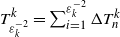 $\smash{T^k_{\varepsilon^{-2}_k}=\sum_{i=1}^{\varepsilon^{-2}_k}\Delta T^k_n}\vphantom{\int^{{A}^{A}}}$
is an independent and identically distributed sum of random variables with mean
 $\varepsilon^2_k$
, we shall use classical large deviations techniques to find, for each
 $q\ge 1$
, a constant C (depending only on q) such that
 $$\begin{equation}
\mathbb{P}\{\delta + T^k_{\varepsilon^{-2}_k} < 1\}\le \exp(-\varepsilon^{-2}_k I^* (1-\delta)),\quad \mathrm{E}|T^k_{\varepsilon^{-2}_k}-1|^q \le C \varepsilon^{2q}_k
\label{eqn38}
\end{equation}
$$
for every
 $k\ge 1$
and
 $\delta\in (0,1)$
. Now, we just need to use (38) into (35), (36), and (37). By observing the estimates (33) and (34), we then conclude the proof.
5.2. Non-Markovian SDE driven by fractional Brownian motion
In this section we analyze Theorem 2 when the reward process
 $Z=F(X)$
is driven by the SDE
 $$\begin{equation}
X(t) = x+ \int_0^t\alpha(s,X)\,{\rm d} s + B_H(t) ,
\label{eqn39}
\end{equation}
$$
where
 $\alpha$
is a bounded non-anticipative functional satisfying Assumption I and
 $B_H$
is the one-dimensional fractional Brownian motion (henceforth abbreviated by FBM) over the interval [0,T] for
 $\frac{1}{2}< H < 1$
. By Theorem 3.4 in [Reference Hu23], we shall represent
 $$B_H(t) = \int_0^t \rho_H(t,s)B(s)\,{\rm d} s,;
\quad 0\le t\le T,$$
where
 $\rho_H(t,s):=\partial_s K_H(t,s)$
and
 $K_H(t,s):= d_Hs^{\frac{1}{2}-H}\int_s^t u^{H-\frac{1}{2}}(u-s)^{H-\frac{3}{2}}\,{\rm d} u$
,
 $0< s < t\le T$
, is the classical square-integrable Volterra kernel that represents FBM. In order to construct an imbedded discrete structure for Z, we need a structure
 $B^k_H$
for
 $B_H$
that converges in
 ${\textbf{B}}^1$
; the natural candidate is
 $$B^k_{H}(t):= \int_0^{\bar{t}_k}\rho_H(\bar{t}_k,s)A^k(s)\,{\rm d} s,;
\quad 0\le t\le T,$$
where we recall that
 $\bar{t}_k$
is given by (6). Due to singularity of the kernel
 $\rho_H$
jointly with the appearance of random times and the piecewise constant process
 $A^k$
, it is not obvious that
 $B^k_H$
fulfills this requirement. The proof of the next result is postponed to the Appendix.
Proposition 3. If
 $\frac{1}{2} < H < 1$
and
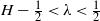 $H-\frac{1}{2} < \lambda < \frac{1}{2}$
, there exists a constant C that depends on H, T, and
 $\lambda$
such that
 \mathrm{E}\sup_{0\le t\le T}|B^k_H(\bar{t}_k) - B_H(t)|\le C\varepsilon_k^{1-2\lambda}$$
for every
 $k\ge 1$
.
The natural candidate for an imbedded discrete structure
 $((Z^k)_{k\ge1},{\cal D})$
w.r.t. (30) is given by
 $$\begin{equation}
Z^k(t) := \sum_{n=0}^{\infty}F(T^k_n, X^k)\mathbf{1}_{\{T^k_n\le t < T^k_{n+1}\}},;
\quad 0\le t\le T ,
\label{eqn40}
\end{equation}
$$
where
 $X^k(0):= x$
and we define recursively
 $$X^{k}(T^k_{n}):= X^{k}(T^k_{n-1}) + \alpha(T^k_{n-1},X^{k})\Delta T^k_{n} +\Delta B^k_{H}(T^k_{n})$$
for
 $1\le n\le e(k,T)$
. We are now able to state the main result of this section. To simplify the presentation we set
 $T=1$
.
Proposition 4. If Assumptions I and II hold for
 $\theta=1$
, X satisfies (39) with
 $\frac{1}{2} < H < 1$
, and
 $\alpha$
is bounded, then
 $((Z^k)_{k\ge 1},{\cal D})$
given by (40) is an imbedded discrete structure for Z. More importantly, for every
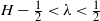 $H-\frac{1}{2} < \lambda < \frac{1}{2}$
, there exists a constant C that depends on
 $\alpha$
, H, and
 $\lambda$
such that
 \label{rateFBMex}
\big|V^k_0 - \sup_{\tau\in \mathcal{T}_0(\mathbb{F})}\mathrm{E}[Z(\tau)]\big| \le C \varepsilon_k^{1-2\lambda}$$
for every
 $k\ge 1$
.
Proof. Let us fix
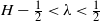 $H-\frac{1}{2} < \lambda < \frac{1}{2}$
. By repeating the same argument presented in Proposition 6.2 in [Reference Leão, Ohashi and Souza28] jointly with the Lipschitz property of F, one can easily check that there exists a constant
 $C(\alpha,\beta,H,\lambda)$
such that
 $$\|Z^k - Z\|_{{\textbf{B}}^1}\le \|F\|C(\alpha,\beta,H,\lambda)\varepsilon^{1-2\lambda}_k$$
for every
 $k\ge 1$
and
 $\beta\in (0,1)$
. By arguing just like the proof of Proposition 2, we have
 $$\big|V^k_0 - \sup_{\tau\in \mathcal{T}_0(\mathbb{F})}\mathrm{E}[Z(\tau)]\big| \le \|F\|C(\alpha,\beta,H,\lambda) \varepsilon^{1-2\lambda}_k + \|F\| \sup_{0\le t\le 1}|X(t\wedge T^k_{e(k,1)}) - X(t)|$$
for every
 $k\ge 1$
. We observe that
 \sup_{0\le t\le 1}|X(t\wedge T^k_{e(k,1)}) - X(t)|\le C(1+ \|X^\eta\|_\infty) |1-T^k_{e(k,1)}| + \sigma \|B_H(\!\cdot\!\wedge T^k_{e(k,1)}) - B_H\|_\infty,$$
where
 $\mathrm{E}\|X\|^{2p}_{\infty}\le C(1+|x_0|^{2p})\exp(C)$
with
 $p\ge 1$
for a constant C depending on
 $B_H$
. For every
 $\varepsilon>0$
, it is well known that there exists
 $G_{\varepsilon}\in \bigcap_{q\ge 1}L^q(\mathbb{P})$
and a deterministic constant C such that
 |B_H(t) - B_H(s)|\le C |t-s|^{(H-\varepsilon)}G_{\varepsilon}~\text{a.s.}$$
for every
 $t,s\in [0,1]$
. Therefore,
 \sup_{0\le t\le 1}|B_H(t) - B_H(t\wedge T^k_{e(k,1)})|\le C |1 - T^k_{e(k,1)}|^{(H-\varepsilon)}G_{\varepsilon}~\text{a.s.}$$
By using (38) and the Cauchy–Schwarz inequality, for every
 $0 < \gamma < H$
there exists a constant C such that
 \mathrm{E}\|B_H(\!\cdot\!\wedge T^k_{e(k,1)}) - B_H\|_\infty\le C \varepsilon_k^{2\gamma}.$$
Taking
 $\gamma + \lambda > \frac{1}{2}$
, we then conclude the proof.
5.3. How to compute optimal values?
It is instructive to end this section with some guidelines on how to concretely produce optimal values in a given (possibly non-Markovian) optimal stopping time problem over a given interval [0,T]. For simplicity of exposition, the dimension of the underlying Brownian motion will be set equal to
 $d=1$
. At first, we recall that the key objects of our methodology are given by (13), (14), and (16), where each random element
 $\mathcal{A}^k_n$
induces an image probability measure
 $\rho^k_n:=\mathbb{P}^k_n$
on
 $\mathbb{S}^n_k$
,
 $n\ge 1$
, where
 $\rho_0$
is just the Dirac concentrated on
 $\textbf{0}$
.
Let
 $\mathbb{Z}^k=\{\mathbb{Z}^k_n;\,\, n=0, \ldots, e(k,T)\}$
be a list of Borel functions that realizes (10). Recall that
 $\mathbb{Z}^k$
must be interpreted as the payoff functional composed with a pathwise version of an imbedded discrete structure (see Definition 1) for a given state that is typically an Euler-type approximation driven by
 $A^k$
. See [Reference Bezerra, Ohashi, Russo and Souza7, Reference Leão, Ohashi and Souza28] for further details. We assume that
 $\mathbb{Z}^k_n\,:\,\mathbb{S}^n_k\rightarrow \mathbb{R} \in L^2(\mathbb{S}^n_k,\rho^k_n)$
for every
 $n=0, \ldots, e(k,T)$
. Let us now select a subset
 $\smash{\{\skew3\widehat{{\textbf{{U}}}}^{\:k}_j;\,\,j=0, \ldots e(k,T)-1 \}}$
of functions such that
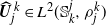 $\smash{\skew3\widehat{{\textbf{{U}}}}^{\:k}_j\in L^2(\mathbb{S}^{j}_k,\rho^k_j)}$
for each
 $j=0, \ldots, e(k,T)-1$
. For each choice of functions, we inductively set
 \label{DPST1}
\left\{\!\!\begin{array}{ll}
\widehat{\tau}^{\:k}_{e(k,T)} & := e(k,T), \\[4pt]
\widehat{\tau}^{\:k}_{j} & := j {1}_{\widehat{G}^k_j} + \tau^{k}_{j+1}{1}_{(\widehat{G}^{k}_j)^c},;
\quad 0\le \kern1ptj \le e(k,T)-1,
\end{array}\right.$$
where
 $\widehat{G}^k_j := \{\mathbb{Z}^k_j (\mathcal{A}^k_j)\ge \widehat{{\textbf{{U}}}}^{k}_j(\mathcal{A}^k_j)\}$
,
 $0\le \kern1ptj\le e(k,T)-1$
, and
 $\widehat{\tau}^{\:k}=\widehat{\tau}^{\:k}_0$
. Here,
 $\skew3\widehat{{\textbf{{U}}}}^{\:k}_j(\!\cdot\!)$
should be interpreted as a suitable approximation of
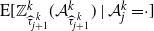 $\mathrm{E}[\mathbb{Z}^k_{\widehat{\tau}^{\:k}_{j+1}}(\mathcal{A}^k_{\widehat{\tau}^{\:k}_{j+1}}) \!\mid\! \mathcal{A}^k_j=\!\cdot]$
for each
 $j=0, \ldots, e(k,T)-~1$
.
The set
 $\{\widehat{\tau}^{\:k}_j;\,\,0\le \kern1ptj \le e(k,T)\}$
induces a set of conditional expectations
 \mathrm{E}[Y^k(\widehat{\tau}^{\:k}_{j+1}) \!\mid\! \mathcal{A}^k_{j}]= \mathrm{E}[\mathbb{Z}^k_{\widehat{\tau}^{\:k}_{j+1}}(\mathcal{A}^k_{\widehat{\tau}^{\:k}_{j+1}})\!\mid\!\mathcal{A}^k_j],;
\quad j=0, \ldots, e(k,T)-1,$$
so that one can postulate
 \max\{\mathbb{Z}^k_0(\textbf{0});\,\, \widehat{{\textbf{{U}}}}^{k}_0(\textbf{0})\}$$
as a possible approximation for (16). Having said that, we are now able to produce a Longstaff–Schwartz-type Monte Carlo scheme as demonstrated in [Reference Bezerra, Ohashi, Russo and Souza7], which we briefly outline here. For further details we refer the reader to [Reference Bezerra, Ohashi, Russo and Souza7].
Given any positive integer N, select
 $\mathcal{H}^k_{N,0}\subset \mathbb{R}$
. For each
 $j=1, \ldots, e(k,T)-1$
, select
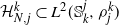 $\smash{\mathcal{H}^k_{N,j}\subset L^2(\mathbb{S}^j_k, \rho^k_j)}$
. The sets
 $\mathcal{H}^k_{N,j}$
,
 $0\le \kern1ptj\le e(k,T)$
(the so-called approximation architectures) possibly depend on N, and their choice is dictated by some a priori information that one possibly has about the continuation values (14). From
 $(\mathcal{A}^k_\ell;\,\,0\le \ell \le e(k,T))$
, generate N independent samples
 \mathcal{A}^k_{0,i}, \mathcal{A}^k_{1,i}, \ldots, \mathcal{A}^k_{e(k,T),i},;
\quad i=1, \ldots, N.$$
This step can be implemented by means of the perfect simulation algorithm developed in [Reference Burq and Jones13]. For a concrete implementation in the context of hedging for European-type options, see [Reference Bonetti, Leão, Ohashi and Siqueira8]. For each
 $\ell=0, \ldots ,e(k,T)$
, let us denote
 {\textbf{{A}}}^k_{\ell N}:=(\mathcal{A}^k_{\ell,1},\mathcal{A}^k_{\ell,2}, \ldots, \mathcal{A}^k_{\ell,N};\,\, \ldots;\,\, \mathcal{A}^k_{e(k,T), 1},\mathcal{A}^k_{e(k,T), 2}, \ldots, \mathcal{A}^k_{e(k,T),N} )$$
with
 $(e(k,T)-\ell+1)N$
factors.
For
 $j=e(k,T)-1$
, we set
 $\widehat{\tau}^{\:k}_{j+1} := \widehat{\tau}^{\:k}_{j+1}({\textbf{{A}}}^k_{(\kern1.5ptj+1)N}) := e(k,T)$
and generate
 \{ (\mathcal{A}^k_{j,i}, (\mathbb{Z}^k_{\widehat{\tau}^{\:k}_{j+1}})_i);\,\,1\le i\le N\},$$
where we define
 $(\mathbb{Z}^k_{\widehat{\tau}^{\:k}_{j+1}})_i:=\mathbb{Z}^k_{e(k,T)}(\mathcal{A}^k_{e(k,T),i})$
,
 $1\le i\le N$
. We then select
 $$\begin{equation}
\skew3\widehat{{\textbf{{U}}}}^{\:k}_{j} := \text{arg min}_{g\in \mathcal{H}^k_{N,j}}\frac{1}{N}\sum_{i=1}^N ((\mathbb{Z}^k_{\widehat{\tau}^{\:k}_{j+1}})_i - g(\mathcal{A}^k_{j,i}) )^2.
\label{eqn41}
\end{equation}
$$
One should notice that
 $\skew3\widehat{{\textbf{{U}}}}^{\:k}_{j}$
is a functional of
 ${\textbf{{A}}}^k_{j N}$
, and we assume the existence of a minimizer (see Remark 4.4 in [Reference Bezerra, Ohashi, Russo and Souza7])
 \label{minimizerMC}\skew3\widehat{{\textbf{{U}}}}^{\:k}_{j}\,:\,\mathbb{S}^{j}_k\times (\mathbb{S}^{j}_k)^N \times\!\cdots\!\times (\mathbb{S}^{e(k,T)}_k)^N\rightarrow \mathbb{R}$$
of (41), which possibly depends on N. With
 $\skew3\widehat{{\textbf{{U}}}}^{\:k}_j$
at hand, we compute
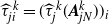 $\widehat{\tau}^{\:k}_{ji} = ( \widehat{\tau}^{\:k}_j ( {\textbf{{A}}}^k_{jN} ) )_i$
, the value that
 $\smash{\widehat{\tau}^{\:k}_{j} =\widehat{\tau}^{\:k}_{j}( {\textbf{{A}}}^k_{jN} )} $
assumes based on the ith sample according to (13). In this case, we set
 $$\begin{equation}
(\mathbb{Z}^k_{\widehat{\tau}^{\:k}_j})_i:=\left\{\!\!
\begin{array}{ll}
\mathbb{Z}^k_j(\mathcal{A}^k_{j,i}) & \hbox{if} \ \widehat{\tau}^{\:k}_{ji}=j , \\[4pt]
\mathbb{Z}^k_{\widehat{\tau}^{\:k}_{(\kern1.5ptj+1)i}}(\mathcal{A}^k_{\widehat{\tau}^{\:k}_{(\kern1.5ptj+1)i},i}) & \hbox{if} \ \widehat{\tau}^{\:k}_{ji} = \widehat{\tau}^{\:k}_{(\kern1.5ptj+1)i} , \\
\end{array}
\right.
\label{eqn42}
\end{equation}
$$
where
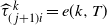 $\widehat{\tau}^{\:k}_{(\kern1.5ptj+1)i}=e(k,T)$
for
 $1\le i\le N$
.
Based on (41) and (42), we then repeat this procedure inductively,
 $j=e(k,T)-2, \ldots, 1, 0$
, to get
 ( \widehat{\tau}^{\:k}_{ji}, \skew3\widehat{{\textbf{{U}}}}^{\:k}_{j}, (\mathbb{Z}^k_{\widehat{\tau}^{\:k}_{j}})_i ),;
\quad 0\le \kern1ptj\le e(k,T),\ 1\le i\le N.$$
For
 $j=0$
, we set
 \widehat{V}_0({\textbf{{A}}}^k_{0N}) := \text{max}\{\mathbb{Z}^k_0(\textbf{0}), \skew3\widehat{{\textbf{{U}}}}^{\:k}_0({\textbf{{A}}}^k_{0N})\}.$$
The above procedure is consistent with the limiting optimal stopping time problem as demonstrated by the following result. It is an immediate consequence of Theorem 4.1 in [Reference Bezerra, Ohashi, Russo and Souza7] and Propositions 2 and 4. In the following, vc denotes the Vapnik–Chervonenkis dimension of a subset.
(H1) For each
 $k\ge 1$
, suppose that
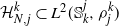 $\mathcal{H}^k_{N,j}\subset L^2(\mathbb{S}^j_k, \rho^k_j)$
and there exists
 $\nu_k$
such that
 $vc(\mathcal{H}^k_{N,j})\le \nu_k < +\infty$
for every
 $j=1, \ldots, e(k,T)-1$
and for every
 $N\ge 2$
.
(H2) For each
 $k\ge 1$
, there exists
 $B_k$
such that
 $\sup\{\|\kern1ptf\|_\infty;\,\, f\in \mathcal{H}^k_{N,j}\}\le B_k < +\infty$
for every
 $j=0, \ldots, e(k,T)-1$
and
 $N\ge 2$
.
By applying Propositions 2 and 4 and Theorem 4.1 in [Reference Bezerra, Ohashi, Russo and Souza7], we arrive at the following result.
Corollary 1. Assume (A1), (A2), (H1), (H2), and the hypotheses of Propositions 2 and 4 hold true. Let us assume the architecture spaces
 $\mathcal{H}^k_{N,j}$
are dense subsets of
 $L^2(\rho^k_j)$
for each
 $j=1, \ldots, e(k,T)-1$
, for each positive integer
 $N\ge 2$
, and
 $k\ge 1$
. Then, for every
 $k\ge 1$
sufficiently large,
 \label{a.sconv2}
\lim_{N\rightarrow +\infty}|\widehat{V}^k_0({\textbf{{A}}}^k_{0N}) - S(0)|= 0~a.s.,$$
where
 $S(0) = \sup_{\tau\in \mathcal{T}_0(\mathbb{F})}\mathrm{E}[Z(\tau)]$
and Z is given by (30).
In order to compute a precise number of steps in our scheme, we just need to apply Propositions 2 and 4 combined with Corollary 4.1 in [Reference Bezerra, Ohashi, Russo and Souza7]. In this case, similar to the classical Markovian case, smoothness of the continuation values
 ${\textbf{{U}}}^{k}_j$
,
 $j=0,\ldots, e(k,T)-1$
, is crucial for choosing approximation spaces to get the most favorable rate of convergence by properly balancing the approximation error and the sample error.
Example 1. For simplicity of exposition let X be the state process given in Section 5.2, where the terminal time, the level of discretization
 $\varepsilon_k$
, the drift, and the payoff are defined, respectively, by
 T=1, \quad \varepsilon_k=\varphi(k),\quad \alpha (s,\eta) = b(\eta(s)),\quad F\,:\,\Lambda\rightarrow \mathbb{R};\,\,\eta \mapsto F(\eta):= h(\eta(1)),$$
for each
 $\eta \in D([0,1];\,\,\mathbb{R})$
and
 $s\in [0,1]$
, where b and h are Lipschitz bounded functions and
 $\varphi\,:\,[0,\infty)\rightarrow [0,\infty)$
is a strictly decreasing function (with inverse
 $\xi$
) such that
 $\sum_{k\ge 1} \varphi^2(k)< \infty$
. We fix
 $\frac{1}{2}< H < 1$
and
 $\lambda$
as described in Proposition 4.
Next, we investigate the global numerical error
 ${\textbf{{e}}} = \text{e}_1+ \text{e}_2$
that may occur in a concrete fully non-Markovian example. The error
 ${\textbf{{e}}}$
can be decomposed as the sum of two terms: the first one (
 $\text{e}_1$
), which we study in this paper, is the discrete-type filtration approximation error; the second one (
 $\text{e}_2$
), which we study in [Reference Bezerra, Ohashi, Russo and Souza7], is related to the numerical approximation of the conditional expectations associated with the continuation values. By using the fact that
 $\alpha$
and F only depend on the present, and performing a similar computation to the one described in the proof of Theorem 5.1 in [Reference Bezerra, Ohashi, Russo and Souza7],
 ${\textbf{B}}^k_n \mapsto {\textbf{{U}}}^k_n({\textbf{B}}^k_n)$
is Lipschitz from
 $\widetilde{\mathbb{S}}^n_k$
to
 $\mathbb{R}$
, where
 $\widetilde{\mathbb{S}}^n_k:= ((0,+\infty)\times B_r(0)) \times\!\cdots\!\times ((0,+\infty)\times B_r(0))$
(n-fold Cartesian product) and
 $B_r(0)$
is an open set centered at the origin with radius
 $r>1$
. We apply Corollary 4.1 in [Reference Bezerra, Ohashi, Russo and Souza7] and Proposition 4 to state that
 $$\begin{align}
\mathrm{E}|\widehat{V}_0({\textbf{{A}}}^k_{0N}) - V^k_0| & = O(\text{log}(N)N^{\frac{-2}{2+e(k,1)-1}}), \label{eqn43}\end{align}
$$
 $$\begin{align}
% \end{equation}
% \begin{equation}
|V^k_0 - S(0)| & = O (\varepsilon_k^{1-2\lambda} ).
\label{eqn44}\end{align}
$$
With the estimates (43) and (44) at hand, we are now able to infer the amount of work (complexity) to recover the optimal value for a given level of accuracy
 ${\textbf{{e}}}$
. Indeed, let us fix
 $0 < \text{e}_1 < 1$
. Equation (44) allows us to find the necessary number of steps related to the discretization as follows. We observe that
 $\smash{\varepsilon^{1-2\lambda}_k \le {\rm e}_1 \Longleftrightarrow k \ge \xi(\text{e}^{\frac{1}{1-2\lambda}}_1)}$
, and with this information at hand we shall take
 $\smash{k^* = \xi(\text{e}^{\frac{1}{1-2\lambda}}_1)}\vphantom{\int^{{A}^{A}}}$
. This produces
 e(k^*,1) = \bigg\lceil \frac{1}{\varphi^{2}(k^*)}\bigg\rceil$$
number of steps associated with the discretization procedure. For instance, if
 $\varphi(k) = 2^{-k}$
,
 $\text{e}_1 = 0.40$
,
 $H=0.6$
, then we shall take
 $\lambda=0.15$
and
 $k^*=-\frac{\text{log}_2~0.40}{0.70}=1.88$
. This produces
 $e(k^*,1)= \lceil 2^{2\times 1.88}\rceil=14$
steps. Of course, as
 $\text{e}_1 \downarrow 0$
, the number of steps
 $e(k^*,1)\uparrow +\infty$
, e.g. if
 $\text{e}_1 = 0.2$
, then
 $k^*=-\frac{\text{log}_2~0.2}{0.70}=3.31$
,
 $e(k^*,1) = 99$
, and so on. For a given prescribed error
 $0 < \text{e}_2 < 1$
and
 $k^{*}$
, (43) allows us to find the necessary number N for the Monte Carlo scheme in such a way that
 $\mathrm{E}|\widehat{V}_0({\textbf{{A}}}^{k^*}_{0N}) - V^{k^*}_0|=O(\text{e}_2)$
.
Appendix A. Proof of Proposition 3. In the following, C is a constant that may differ from line to line. Let us denote
 $$\begin{align*}
\rho_{H,1}(t,s) & = t^{(H-\frac{1}{2})}s^{(\frac{1}{2}-H)}(t-s)^{(H-\frac{3}{2})}, \\ % \quad
\rho_{H,2}(t,s) & = s^{(-H-\frac{1}{2})}\int_s^tu^{(H-\frac{3}{2})}(u-s)^{(H-\frac{1}{2})}\,{\rm d} u
\end{align*}
$$
for
 $ 0 < s <t$
. Clearly, there exists a constant C that depends on T such that
 $$\begin{equation}
|\rho_H(t,s)|\le C \{\rho_{H,1}(t,s) + \rho_{H,2}(t,s)\}
\label{eqn45}
\end{equation}
$$
for
 $ 0 < s <t$
. The triangle inequality and the Hölder property of FBM yield
 $$\begin{equation}
\sup_{0\le t\le T}|B^k_H(\bar{t}_k) - B_H(t)|\le\sup_{0\le t\le T}|B^k_H(\bar{t}_k) - B_H(\bar{t}_k)| + \|B_H\|_{H-\eta} \bigg(\bigvee_{n=1}^{N^k(T)} \Delta T^k_n\bigg)^{H-\eta}~\text{a.s.}
\label{eqn46}
\end{equation}
$$
for every
 $0 < \eta < H$
, where
 $\|\cdot\|_{\theta}$
denotes the Hölder norm for
 $0 < \theta \le 1$
. Clearly,
 $$\begin{equation}
\sup_{0\le t\le T}\int_0^{\bar{t}_k} \rho_{H,1}(\bar{t}_k,s)|A^k(s) - B(s)|\,{\rm d} s\le \varepsilon_k T^{H-\frac{1}{2}}~\text{a.s.}
\label{eqn47}
\end{equation}
$$
The delicate component is
 $\int_0^{\bar{t}_k} \rho_{H,2}(\bar{t}_k,s)|A^k(s) - B(s)|\,{\rm d} s$
. Let us fix
 $p>1$
such that
 $$\begin{equation}
\frac{1}{2} + \frac{1}{p} > \frac{1}{2} > \lambda > \frac{1}{p} + H -\frac{1}{2} , % .
\label{eqn48}
\end{equation}
$$
so that we must have
 $p > \frac{1}{1-H}> 2$
. Let
 $q>1$
be a conjugate exponent such that
 $(-\frac{1}{2}-H+\lambda)q + 1 >0$
. The choice (48) implies that
 \mathrm{E}\bigg\{\int_0^u s^{-\lambda p}|A^k(s)-B(s)|^p\,{\rm d} s\bigg\}^{\frac{1}{p}}< \infty$$
for every
 $0\le u\le T$
. We observe that
 $$\begin{align*}\label{inn1}
\sup_{0\le t\le T}\int_0^{\bar{t}_k}\rho_{H,2}(\bar{t}_k,s)|A^k(s)-B(s)|\,{\rm d} s & \le C \int_0^{T}u^{\lambda -1+ \frac{1}{q}}(d_k(u))^{\frac{1}{p}}u^{H-\frac{3}{2}}\mathbf{1}_{\{N^k(u)>0\}}\,{\rm d} u\\
% & &\\
& \quad + C \int_0^{T}u^{\lambda-1+\frac{1}{q}}(d_k(u))^{\frac{1}{p}}u^{H-\frac{3}{2}} \mathbf{1}_{\{N^k(u)=0\}} \,{\rm d} u,
\end{align*}
$$
where C only depends on H, and
 $$d_k(u):= \int_0^u s^{-\lambda p}|A^k(s)-B(s)|^p\,{\rm d} s.$$
To shorten the notation, let us denote
 J^k(u) = \mathrm{E}\bigg[\int_0^{T^k_{N^k(u)+1}} s^{-\lambda p}|A^k(s)-B(s)|^p\,{\rm d} s\bigg]\mathbf{1}_{\{N^k(u)>0\}}.$$
We observe that
 d_k(u)\mathbf{1}_{\{N^k(u)=0\}}\le \|B\|^p_{\lambda}u{1}_{\{N^k(u)=0\}},\quad d_k(u)\mathbf{1}_{\{N^k(u)>0\}}\le J^k(u)$$
a.s. for every
 $u\in [0,T]$
. Let us now estimate
 $J^k(u)$
for a given
 $u\in (0,T]$
. A lengthy but straightforward calculation based on the strong Markov property of the shifted Brownian motion over the stopping times
 $T^k_n$
yields
 $$\begin{align*}
\mathrm{E}[J^k(u)] & \le \mathrm{E}\bigg[\sum_{n=1}^{2N^k(u)}\int_{0}^{\Delta T^k_n}|v+T^k_{n-1}|^{-\lambda p}|B(v+T^k_{n-1})-B(T^k_{n-1})|^p\,{\rm d} v\bigg] \\
% & &\\
& = C \mathrm{E}[[A^k](u)]\varepsilon_k^{2(-\lambda p+ \frac{p}{2})}\\
% & &\\
& \le C\mathrm{E}[\sup_{0\le \ell \le u}|B(\ell)|^2]\varepsilon_k^{2(-\lambda p+ \frac{p}{2})}\le Cu\varepsilon_k^{2(-\lambda p+ \frac{p}{2})}
\end{align*}
$$
for a constant C that depends only on H. Then,
 $$\mathrm{E}(d_k(u))^{\frac{1}{p}}\le C u^{\frac{1}{p}}\varepsilon_k^{2(-\lambda+\frac{1}{2})} + (\mathrm{E}\|B\|^{\gamma p}_\lambda)^{\frac{1}{p\gamma}} \mathbb{P}^{\frac{1}{\beta p}}\{N^k(u)=0\} u^{\frac{1}{p}}$$
for a constant C that depends on
 $(\lambda,p)$
, where
 $\gamma,\beta>1$
are conjugate exponents. Moreover,
 \mathbb{P}^{\frac{1}{p\beta}}\{N^k(u)=0\}\le C u^{-\frac{1}{p\beta}}\varepsilon_k^{\frac{2}{p\beta}},;
\quad u >0,\ p\beta >2,$$
for a constant C that depends only on
 $p\beta$
. This implies that
 $$\begin{equation}
\mathrm{E}\sup_{0\le t\le T}\int_0^{\bar{t}_k}\rho_{H,2}(\bar{t}_k,s)|A^k(s)-B(s)|\,{\rm d} s\le C T^{H-\frac{1}{2}+\lambda}\varepsilon_k^{2(-\lambda+\frac{1}{2})} + C\varepsilon_k^{\frac{2}{p\beta}}T^{H-\frac{1}{2}+\lambda-\frac{1}{p\beta}}
\label{eqn49}
\end{equation}
$$
by adjusting
 $\frac{1}{p\beta} < \lambda < \frac{1}{2}$
. Summing up the steps (45), (46), (47), and (49), and using Fernique’s theorem, Lemma 2.2 in [Reference Leão, Ohashi and Simas27], and Hölder’s inequality, there exists a constant
 $C = C(\theta,H,a,b,\lambda,\beta,\eta)$
such that
 $$\mathrm{E}\sup_{0\le t\le T}|B^k_H(\bar{t}_k) - B_H(t)|\le C(\theta,H,a,b,\lambda,\beta,\eta)(\varepsilon_k^{2(H-\eta)-\frac{2}{b}(1-\theta)} + \varepsilon^{1-2\lambda}_k + \varepsilon^{\frac{2}{p\beta}}_k)$$
for every
 $a,b >1$
conjugate exponents,
 $\theta\in (0,1)$
,
 $(\lambda,p)$
satisfying (48),
 $\beta>1$
, and
 $\eta \in (0,H)$
. Finally, we can choose
 $(\eta,\theta,b)$
in such a way that
 1 > 2\lambda>2\eta +\frac{2}{b}(1-\theta),$$
and since
 $2H > 1$
, we then have
 $1-2\lambda < 2H - ( 2\eta +\frac{2}{b}(1-\theta))$
. We can also choose
 $(\kern1ptp,\beta)$
in such a way that
 \frac{1}{2}> \lambda > \frac{1}{2}-\frac{1}{p\beta}> \frac{1}{p} + H-\frac{1}{2},$$
and in this case
 $1-2\lambda < \frac{2}{p\beta}$
. This concludes the proof.
Acknowledgements
Alberto Ohashi and Francesco Russo acknowledge the financial support of Math Amsud grant 88887.197425/2018-00. Alberto Ohashi acknowledges ENSTA ParisTech for their hospitality and CNPq-Bolsa de Produtividade de Pesquisa grant 303443/2018-9. The authors would like to thank the referees for the careful reading and suggestions which considerably improved the presentation of this paper.


