


1. Introduction
The multi-scale nature of particle-laden flows gives rise to rich and complex physics that have significant impact on natural and industrial processes. Particularly, inertial particle motion at moderate to high mass loadings is intimately coupled to the carrier fluid flow (Elgobashi Reference Elgobashi, Balachandar and Prosperetti2006). Eulerian–Lagrangian (EL) methods (also referred to in the literature as computational fluid dynamics–discrete element modelling or point particle methods) have gained substantial traction for modelling such strongly coupled particle-laden flows due to a balance between speed and resolution (see Cundall & Strack Reference Cundall and Strack1979; Tsuji, Kawaguchi & Tanaka Reference Tsuji, Kawaguchi and Tanaka1993; van der Hoef et al. Reference van der Hoef, van Sint Annaland, Deen and Kuipers2008; Capecelatro & Desjardins Reference Capecelatro and Desjardins2013). Since EL methods do not resolve the boundary layer around each particle, they enable grid spacings of the order of or larger than the particle diameter. The reduced resolution in EL methods requires a model for the fluid–particle force (i.e. drag), which generally depends upon the undisturbed fluid velocity. In many cases, two-way coupling can lead to self-induced disturbances (Ireland & Desjardins Reference Ireland and Desjardins2017; Horwitz & Mani Reference Horwitz and Mani2018; Balachandar, Liu & Lakhote Reference Balachandar, Liu and Lakhote2019) or neighbour-induced disturbances (Akiki, Jackson & Balachandar Reference Akiki, Jackson and Balachandar2017) that affect the observed accuracy of an EL method. By contrast, particle-resolved direct numerical simulation (PR–DNS) does not require a model for the interphase force since the detailed flow around each particle is captured. For strongly coupled flows with inertial particles, increasing the quantitative agreement between EL methods and PR–DNS requires critical assessment of the drag force model. Existing drag force closures developed for EL methods typically capture the mean fluid–particle force experienced by an assembly of particles. Therefore, the variance in drag force, arising from neighbour-induced, sub-grid fluid velocity fluctuations (referred to as pseudo-turbulent kinetic energy; PTKE), is generally ignored. However, recent works have highlighted the importance of PTKE in particle-laden flows; see the closed-form model in Mehrabadi et al. (Reference Mehrabadi, Tenneti, Garg and Subramaniam2015) and transport equations in Shallcross, Fox & Capecelatro (Reference Shallcross, Fox and Capecelatro2020). Establishing connections between the drag force fluctuations and particle fluctuations (granular temperature and mean-square displacement) creates a platform for development of an EL drag framework that may be informed by the local PTKE.
When comparing EL and PR–DNS, Kriebitzsch, van der Hoef & Kuipers (Reference Kriebitzsch, van der Hoef and Kuipers2013) highlighted that the mean drag and drag variance were under-predicted by EL methods. More recently, Tenneti, Mehrabadi & Subramaniam (Reference Tenneti, Mehrabadi and Subramaniam2016) demonstrated that EL methods with a mean drag force closure are incapable of capturing the steady granular temperature observed in PR–DNS with freely evolving particles. Numerous works with PR–DNS have since emphasized that flow past a collection of monodisperse spheres will yield drag forces that are normally distributed (Akiki, Jackson & Balachandar Reference Akiki, Jackson and Balachandar2016; Esteghamatian et al. Reference Esteghamatian, Bernard, Lance, Hammouti and Wachs2017; Huang et al. Reference Huang, Wang, Zhou and Li2017). Akiki et al. (Reference Akiki, Jackson and Balachandar2016) demonstrated that significant lift forces are generated by neighbour-induced pressure asymmetry. They found that, for static particle assemblies, the lift forces are also normally distributed and the variance in lift is similar in magnitude to the variance in drag. Results obtained by Esteghamatian et al. (Reference Esteghamatian, Bernard, Lance, Hammouti and Wachs2017), with freely evolving particles, also indicated that large ‘drift’ forces were present in the transverse direction of their fluidized bed simulations. It has thus become increasingly clear that the variance of the drag force distribution, arising from fluid disturbances by neighbouring particles, provides a source for fluctuating particle velocity and dispersion in EL methods. While the emphasis here is placed on EL methods, it is noted that sources to granular temperature resulting from interphase drag fluctuations also play a crucial role in Euler–Euler (EE) methods for gas–solids flows; see kinetic theories derived in Koch (Reference Koch1990); Koch & Sangani (Reference Koch and Sangani1999) and Garzó et al. (Reference Garzó, Tenneti, Subramaniam and Hrenya2012).
Previous efforts to account for the drag force distribution in EL methods may be broadly grouped into deterministic and stochastic approaches. In the former, the drag force experienced by a given particle is directly mapped to its pairwise neighbour interactions (Akiki et al. Reference Akiki, Jackson and Balachandar2017), requiring that the relative position of each particle be known when computing the drag force. It is worth noting that the aforementioned information is available in an EL framework but not in an EE framework where the solids are treated as a continuum. By contrast, stochastic approaches aim to capture the particle statistics (granular temperature and dispersion) resulting from neighbour-induced drag force fluctuations. Similar to pioneering works with turbulent single-phase flows (Haworth & Pope Reference Haworth and Pope1986; Sawford Reference Sawford1991; Pope Reference Pope1994, Reference Pope2002), stochastic approaches for multiphase flows often employ simple Langevin equations (Iliopoulos, Mito & Hanratty Reference Iliopoulos, Mito and Hanratty2003; Pozorski & Apte Reference Pozorski and Apte2009; Pai & Subramaniam Reference Pai and Subramaniam2012; Tenneti et al. Reference Tenneti, Mehrabadi and Subramaniam2016). However, the random increments in a stochastic approach may be introduced into the particle properties at various ‘levels’ (position, velocity or force), leading to different dynamical responses for the granular temperature and dispersion.
In general, position Langevin (PL) equations are utilized for non-inertial tracer particles where the relaxation of the particle velocity due to drag is not resolved; see Papavassiliou & Hanratty (Reference Papavassiliou and Hanratty1997) and Na, Papavassiliou & Hanratty (Reference Na, Papavassiliou and Hanratty1999) for single-phase and Metzger, Rahli & Yin (Reference Metzger, Rahli and Yin2013) and Lattanzi, Yin & Hrenya (Reference Lattanzi, Yin and Hrenya2020) for multiphase examples. However, a variety of velocity Langevin (VL) approaches have been employed for inertial particles. When examining dilute particles in isotropic turbulence, Pozorski & Apte (Reference Pozorski and Apte2009) considered a Langevin equation for the fluctuating fluid velocity that is closed with the sub-grid kinetic energy and sub-grid fluid time scale. By contrast, for moderate solids loading and Reynolds number, Tenneti et al. (Reference Tenneti, Mehrabadi and Subramaniam2016) considered a Langevin equation for the fluctuating particle velocity and related the model inputs to PR–DNS statistics. To appropriately capture the interphase turbulent kinetic energy transfer in dilute particle-laden turbulent flows, Pai & Subramaniam (Reference Pai and Subramaniam2012) developed a coupled system of Langevin equations for the fluctuating fluid velocity and the fluctuating particle velocity. When applying a random force contribution, referred to here as a force Langevin (FL), fewer considerations have been given. Andrews, Loezos & Sundaresan (Reference Andrews, Loezos and Sundaresan2005) considered a fluctuating force Langevin in coarse-grid EE simulations of a vertical riser and informed the model inputs (force time scale and variance) with fine-grid EE simulations. Esteghamatian et al. (Reference Esteghamatian, Euzenat, Hammouti, Lance and Wachs2018) implemented a Langevin model for the fluctuating drag coefficient into their EL framework and utilized PR–DNS to obtain model closure. For liquid–solid beds with homogeneous fluidization, improved predictions with the stochastic drag coefficient model were reported. However, for gas–solid beds with heterogeneous fluidization, Esteghamatian et al. (Reference Esteghamatian, Euzenat, Hammouti, Lance and Wachs2018) suggest that the EL method already captures dynamic coherent structures (e.g. clusters or bubbles) and the stochastic force formulation offers little benefit. The stochastic drag model of Esteghamatian et al. (Reference Esteghamatian, Euzenat, Hammouti, Lance and Wachs2018) was also utilized by Rao & Capecelatro (Reference Rao and Capecelatro2019) for EL simulations of a dense particle bed subject to fluid shearing (sub-aqueous sedimentary flow). Similar to Esteghamatian et al. (Reference Esteghamatian, Euzenat, Hammouti, Lance and Wachs2018), Rao & Capecelatro (Reference Rao and Capecelatro2019) reported improved predictions for bed height when the flow was near the onset of erosion, but minor benefit was observed at higher flow rates.
Some ambiguity has persisted in the particle-laden flow literature when selecting a Langevin framework. Particularly, FL approaches have admittedly been ad hoc proposals. For single-phase turbulent flows, seminal contributions have been made to acceleration Langevin approaches (Sawford Reference Sawford1991). As a result, such frameworks have been placed on a much firmer theoretical foundation and are capable of reproducing statistics obtained from single-phase DNS (Yeung & Pope Reference Yeung and Pope1989). With an ultimate goal of model development for EL methods, we present a rigorous derivation of the particle velocity variance (granular temperature) and dispersion (mean-square displacement) resulting from a PL, VL and FL equation. Solutions derived herein provide a basis for comparison with PR–DNS results and allow an informed decision to be made as to which Langevin equation is appropriate for a given flow. Analytical solutions are verified against numerical integration of the corresponding stochastic differential equation (SDE). We start with Stokes drag, collisionless particles and an isotropic diffusion tensor. However, it is emphasized that the assumptions allow closed-form solutions to be obtained that highlight similarities and differences between the methods, and are not inherent restrictions of any of the Langevin equations.
In § 3 it is shown that random increments on the particle position (PL) leads to dispersion behaviour that follows simple diffusion and gives no direct control of the granular temperature. In § 4 we consider random increments on the particle velocity (VL) and show that it leads to dispersion behaviour with a ballistic and diffusive regime. If the particles are initialized with a Maxwellian velocity distribution whose variance matches the steady velocity variance, then the ballistic regime follows the classic result of Taylor (Reference Taylor1922). However, if the particles are initialized with zero velocity, then additional time scales are introduced into the ballistic regime that act to inhibit particle dispersion due to the temporal growth of granular temperature. In contrast to PL, VL allows for direct control of the velocity variance since sources (neighbour-induced force fluctuations) and dissipation (due to drag) are present in the granular temperature balance; see discussion in Tenneti et al. (Reference Tenneti, Mehrabadi and Subramaniam2016). However, VL treats the fluctuating drag force, due to the presence of neighbouring particles, as a zero memory process. By contrast, the fluctuating drag force experienced by a given particle may persist for finite time scales in some systems. Random increments on the particle force (FL) are considered in § 5 and it is shown that FL allows for fluctuating drag forces with finite memory. Additionally, random increments in FL physically correspond to the fluctuating drag force extracted from PR–DNS, which have been shown to be well approximated by a Gaussian distribution (Akiki et al. Reference Akiki, Jackson and Balachandar2016; Esteghamatian et al. Reference Esteghamatian, Bernard, Lance, Hammouti and Wachs2017; Huang et al. Reference Huang, Wang, Zhou and Li2017). The ratio of the Stokes response time,  $\tau _p$, to the force time scale,
 $\tau _F$, defines a Stokes number for the fluctuating force given by
 $St_F=\tau _p/\tau _F$. At large
 $St_F$, FL converges to VL. For small
 $St_F$, FL leads to larger velocity variances and dispersion due to the persistence of force–velocity correlations. Both the velocity variance and dispersion may be controlled with the FL framework and the inputs have physical connections to force statistics available in PR–DNS.
2. System under consideration
Three types of Langevin equations are discussed in the following sections and the evolution equations for velocity variance and dispersion are derived. The present study considers dispersion from a line source in a statistically homogeneous flow (mean particle velocity is homogeneous). We motivate the case study by considering particles in an EL method, where unresolved fluid velocity fluctuations (PTKE) give rise to drag force fluctuations that induce velocity variance and particle dispersion. In all cases, we consider an initial impulse of particles centred at  $x=0$ and uniformly distributed in the y-direction. The particle velocities are initialized as either (i) all initially static i.e.
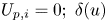 $U_{p,i}=0; \ \delta (u)$ or (ii) a Maxwellian velocity distribution
 $\mathcal {N}[0,\sigma ^2]$; where
 $\mathcal {N}$ is a normal distribution with zero mean and variance
 $\sigma ^2$.
Analytical solutions derived here are compared to results obtained from numerical solutions of the Langevin equations. In the present study, numerical integration of the Langevin equations is considerably more straightforward than deriving the exact solution. For this reason, simulation results are considered less error prone and included here as a confirmation of the analytical results. The SDEs are integrated with an Euler–Maruyama method (Kloeden & Platen Reference Kloeden and Platen1992) with  $10^{5}$ particles, and the smallest time scale of the system is resolved by 25 time steps. We do not consider particle collisions in the present work, and thus, the two relevant time scales are those associated with mean drag defined as
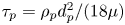 $\tau _p = \rho _p d_p^2/(18 \mathrm {\mu })$ and the fluctuating drag force
 $\tau _F$; where
 $\rho _p$ is the particle density,
 $d_p$ is the particle diameter and
 $\mathrm {\mu }$ is the fluid dynamic viscosity. The computational domain is a doubly periodic rectangular grid with aspect ratio of 6. Probability distributions for the particle phase were obtained by decomposing the length of the domain into 501 bins and computing the particle number density within each bin. It is worth noting that particle dispersion here is one-dimensional in nature and particles do not interact with the periodic
 $x$-direction boundaries. The two-dimensional domain merely allows for more intuitive visualization; see figure 1 for example.
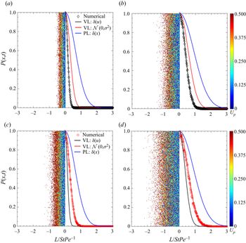
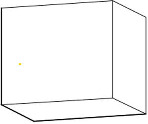
(a,b) Analytical and numerical predictions for particle dispersion with the VL framework and an impulse velocity condition. (c,d) Analytical and numerical predictions for particle dispersion with the VL framework and a Maxwellian velocity condition. In all cases,  $St = 5$,
 $Pe = 2$ and the particles (left half of images) are coloured by the magnitude of their velocity in the
 $x$-direction.
 $(a{,}c)\,\, t = 0.500, (b{,}d)\,\, t = 1.000.$

As noted above, the theory here treats particles as collisionless and emphasis is placed on hydrodynamic force fluctuations. For inelastic granular flows, a Chapman–Enskog expansion shows that the granular temperature follows a hydrodynamic equation where acceleration is balanced by generation due to shear work, diffusion and dissipation from inelastic collisions (Garzó & Dufty Reference Garzó and Dufty1999). Extending the kinetic theory to account for fluid phase effects shows that additional source and sink terms arise from hydrodynamic forces (Koch & Sangani Reference Koch and Sangani1999; Garzó et al. Reference Garzó, Tenneti, Subramaniam and Hrenya2012). For a homogeneous flow of elastic particles, the granular temperature balance only retains the hydrodynamic source and sink terms (Tenneti et al. Reference Tenneti, Mehrabadi and Subramaniam2016). It is this fluctuation dissipation relation that we probe via stochastic methods. In regard to dispersion, collisions will affect particle migration and the closures derived here should be viewed as upper bounds that are more appropriate for dilute flows. While not considered here, the method outlined by Pai & Subramaniam (Reference Pai and Subramaniam2009) would provide a path for including the effect of a uniform shear flow.
3. Position Langevin
Evolution of a particle's position follows from the definition of its velocity
 \begin{equation} \frac{\textrm{d} \boldsymbol{X}_{p,i}}{\textrm{d} t} = \boldsymbol{U}_{p,i}, \end{equation}
where  $\boldsymbol {X}_{p,i}$ is the position of particle
 $i$ and
 $\boldsymbol {U}_{p,i}$ is the velocity of particle
 $i$. Introducing random fluctuations into (3.1) leads to the following SDE
 \begin{equation} \mathrm{d}\boldsymbol{X}_{p,i} = \boldsymbol{U}_{p,i}\, \mathrm{d}t + {\bar{\boldsymbol{\mathsf{b}}}}(\boldsymbol{X},t)\, \mathrm{d}\boldsymbol{W}_t, \end{equation}
where  ${\bar {\boldsymbol{\mathsf{b}}}}(\boldsymbol {X},t)$ is the diffusion tensor and
 $\mathrm {d}\boldsymbol {W}_t$ is a Wiener process increment. Utilizing Itô calculus, (3.2) corresponds to the following Fokker–Planck (FP) equation (detailed derivations of the Fokker–Planck equation are not provided here but the interested reader is referred to chapter 4 of Risken & Frank (Reference Risken and Frank1996).)
 \begin{equation} \frac{\partial P(\boldsymbol{u},\boldsymbol{x};t|\boldsymbol{v},\boldsymbol{y},s)}{\partial t} + \sum_{i=1}^{N}\frac{\partial u_i P}{\partial x_i} = \sum_{i=1}^{N} \sum_{j=1}^{M}\frac{\partial D_{ij}P}{\partial x_i x_j}, \end{equation}
where  $P(\boldsymbol {u},\boldsymbol {x};t|\boldsymbol {v},\boldsymbol {y},s)$ is the probability distribution conditioned on the initial condition for velocity
 $\boldsymbol {v}$, position
 $\boldsymbol {y}$ and time
 $s$,
 $u_i$ is the particle velocity and
 ${\bar {\boldsymbol{\mathsf{D}}}}={\bar {\boldsymbol{\mathsf{b}}}}{\bar {\boldsymbol{\mathsf{b}}}}^{\boldsymbol{\mathsf{T}}}/{2}$. For a constant diffusivity tensor
 ${\bar {\boldsymbol{\mathsf{D}}}}$, (3.3) follows an advection–diffusion equation.
Here, we consider the particle diameter  $d_p$, Stokes response time
 $\tau _p$ and terminal velocity
 $V_T=\tau _p g(1- \rho _f/\rho _p)$ as reference scales, where
 $\rho _f$ is the fluid density. From these scales, we define the Stokes number
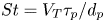 $St = V_T \tau _p/d_p$ and Péclet number
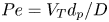 $Pe = V_T d_p/D$. Taking
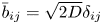 $\bar {b}_{ij} = \sqrt {2D}\delta _{ij}$, we obtain a dimensionless form for (3.2)
 \begin{equation} \mathrm{d}\boldsymbol{X}_{p,i} = St\, \boldsymbol{U}_{p,i} \,\mathrm{d}t +\sqrt{2 St\,Pe^{-1}} \,\mathrm{d}\boldsymbol{W}_t \end{equation}
that leads to the following Fokker–Planck equation
 \begin{equation} \frac{\partial P}{\partial t} + St\, \boldsymbol{\nabla} \boldsymbol{\cdot} (\boldsymbol{u} P) = St\,Pe^{-1} \Delta(P). \end{equation}
In general, the Fokker–Planck equation poses a significant challenge to analytical methods. However, closed-form solutions are highly instructive when possible. For one dimension and constant velocity, a change of reference frame ( $\eta = x - St\, u t$) yields the diffusion equation
 \begin{equation} \frac{\partial P}{\partial t} = St\,Pe^{-1}\frac{\partial^{2} P}{\partial \eta^{2}}. \end{equation}
An initial impulse at the origin,  $\delta (x)$, leads to the classic heat kernel solution
 \begin{equation} P(\eta;t) = \frac{1}{\sqrt{4{\rm \pi} St\,Pe^{-1} t}}\exp\left(-\frac{\eta^2}{4St\,Pe^{-1}t}\right), \end{equation}
or  $\mathcal {N}[0, 2 St\,Pe^{-1}t]$ for shorthand. Equation (3.6) will serve as the starting point in the following subsections and connections will be made to (3.7).
3.1. Fluctuating velocity (PL)
Since random increments are introduced at the particle position level, the PL framework does not provide a direct source or sink to granular temperature in the homogeneous mean velocity cases considered here. However, we note that granular temperature may be generated indirectly by utilizing a PL method in conjunction with a soft-sphere contact model (commonly employed within EL frameworks) or by kinetic streaming of particles within inhomogeneous flows. Specifically, random displacements are unaware of the net force vector exerted on a particle; and thus, particle overlap may be induced by position fluctuations, thereby leading to artificially high restorative forces during a collision. The indirect generation of velocity fluctuations with a soft-sphere contact model is non-physical and quantifying this phenomenon is not considered here. Therefore, we do not consider the role of velocity variance in a PL framework.
3.2. Dispersion (PL)
The variance in position given by  $\mathrm {Var}(x) = \langle (x - \langle x \rangle )^2 \rangle$ is utilized here to characterize particle dispersion, for which the first two moments
 $\langle x \rangle; \ \langle x^2 \rangle$ are of great significance. The
 $\langle \cdot \rangle$ notation employed here indicates an ensemble average over all the particles and at each instance in time, although different definitions for the mean may be adopted depending upon the solution method. Higher dimension distributions will arise in subsequent sections, leading to conditional averages – e.g.
 $\langle x \langle u|x\rangle \rangle$ reads as the ensemble average of the product of position and velocity conditioned on position. When computing moments of the Fokker–Planck equation, the following relations are useful
 \begin{gather} \int x^n \frac{\partial P}{\partial t} \,\textrm{d}x = \frac{\textrm{d} \langle x^n \rangle}{\textrm{d} t}, \end{gather}
 \begin{gather} \int x^n \frac{\partial P}{\partial x} \,\textrm{d}x \equiv \int \left[\frac{\partial x^nP}{\partial x} - nx^{n-1}P\right] \,\textrm{d}x = -n\langle x^{n-1} \rangle, \end{gather}
 \begin{gather} \int x^n \frac{\partial^{2} P}{\partial x^{2}} \,\textrm{d}x \equiv \int \left[\frac{\partial }{\partial x}\left(x^n \frac{\partial P}{\partial x}\right) - n\frac{\partial x^{n-1}P}{\partial x} + n(n-1)x^{n-2}P\right] \,\textrm{d}x = n(n-1)\langle x^{n-2} \rangle, \end{gather}
where integration is performed over the real line and the last equalities in (3.8b) and (3.8c) are obtained with integration by parts and decay of the distribution function ( $\lim _{x\rightarrow \pm \infty } x^n P = 0$). (Similar approaches are employed when taking moments of the Boltzmann equation; see chapter 9 of Vincenti & Kruger (Reference Vincenti and Kruger1975). Additionally, the Gaussian functions obtained here can be shown to decay faster than a polynomial of order
 $n$.) Utilizing (3.8a)–(3.8c), the first and second moments of (3.6) follow
 \begin{gather} \frac{\textrm{d} \langle x \rangle}{\textrm{d} t} = 0, \end{gather}
 \begin{gather} \frac{\textrm{d} \langle x^2 \rangle}{\textrm{d} t} = 2St\,Pe^{-1}. \end{gather}
Employing the impulse initial condition when integrating (3.9a)–(3.9b) allows for evaluation of the position variance
 \begin{equation} \langle \left(x - \langle x \rangle \right)^2 \rangle =2St\,Pe^{-1}t. \end{equation}
Equation (3.10) shows that the dispersion obtained with a PL treatment is consistent with the known solution in (3.7) – i.e. random increments in particle position yield a diffusion process. Equation (3.10) connects the mean-squared displacement to diffusion in one dimension but will be multiplied by the dimensionality  $d$ for isotropic diffusion in higher dimensions.
Returning (3.10) to dimensional form may be completed in a straightforward manner. We first note that  $St\,Pe^{-1} = D \tau _p/d_p^2$. Multiplying the right-hand side of (3.10) by
 $d_p^2$ and replacing
 $t$ with
 $t/\tau _p$, we obtain the classic result:
 $\mathrm {Var}(x) = 2Dt$.
4. Velocity Langevin
Since collisions are not considered here, the relevant forces acting on the particle are due to interphase drag,  $\boldsymbol {F}_{{d},i}$. In general, the drag force is proportional to the slip velocity
 $\boldsymbol {F}_{{d},i} = f(\phi ,Re_m) (\boldsymbol {u}_f - \boldsymbol {U}_{p,i})$, where
 $f(\phi ,Re_m)$ is a function of the solids volume fraction
 $\phi$ and particle Reynolds number
 $Re_m=((1-\phi ) d_p \rho _f |u_f - U_{p,i}|)/\mathrm {\mu }$. Established correlations for the drag force at varying Reynolds number and solids loading may be found in Gidaspow (Reference Gidaspow1994), Hill, Koch & Ladd (Reference Hill, Koch and Ladd2001), Beetstra, van der Hoef & Kuipers (Reference Beetstra, van der Hoef and Kuipers2007), Tenneti, Garg & Subramaniam (Reference Tenneti, Garg and Subramaniam2011) and Rubinstein, Derksen & Sundaresan (Reference Rubinstein, Derksen and Sundaresan2016). For Stokes flow, the system of SDEs for position and velocity is
 \begin{gather} \mathrm{d}\boldsymbol{X}_{p,i} = \boldsymbol{U}_{p,i}\,\mathrm{d}t, \end{gather}
 \begin{gather} \mathrm{d}\boldsymbol{U}_{p,i} = \frac{\boldsymbol{u}_f - \boldsymbol{U}_{p,i}}{\tau_p} \mathrm{d}t + {\bar{\boldsymbol{\mathsf{b}}}}(\boldsymbol{V},\boldsymbol{X};t) \mathrm{d}\boldsymbol{W}_t.\end{gather}
In the absence of collisions, the velocity SDE in (4.1b) contains a restoring force that relaxes the particle velocity towards the fluid velocity  $\boldsymbol {F}_{{d},i}/m_{p,i} = (\boldsymbol {u}_f-\boldsymbol {U}_{p,i})/\tau _p$ and a random fluctuation
 ${\bar {\boldsymbol{\mathsf{b}}}}\,\mathrm {d}\boldsymbol {W}_t$.
When defining the driving force for drag, we utilize the instantaneous particle velocity  $\boldsymbol {U}_{p,i}$, which is resolved in an EL method. When considering a VL approach, Tenneti et al. (Reference Tenneti, Mehrabadi and Subramaniam2016) utilized the mean particle velocity
 $\left \langle \boldsymbol {U}_{p}\right \rangle$ to define the driving force for mean drag. By doing so, Tenneti et al. (Reference Tenneti, Mehrabadi and Subramaniam2016) was able to introduce a different time scale for the relaxation of particle velocity fluctuations
 $\gamma$. This new time scale implies that the viscous dissipation of particle velocity fluctuations is fundamentally different than the drag force for mean particle velocity. Similarly, the dissipation of granular temperature due to viscous effects has been probed via multi-pole (Sangani & Mo Reference Sangani and Mo1996) and lattice Boltzmann simulations (Wylie, Koch & Ladd Reference Wylie, Koch and Ladd2003). These works also suggest that the viscous dissipation of particle velocity fluctuations can depart from mean drag and will scale with solids volume fraction and Reynolds number
 $Re_T=(\rho _f d_p \sqrt {T})/\mathrm {\mu }$ based on granular temperature
 $T$ (see
 $R_{{diss}}(\phi )$ in Sangani et al. Reference Sangani, Mo, Tsao and Koch1996; Koch & Sangani Reference Koch and Sangani1999; Wylie et al. Reference Wylie, Koch and Ladd2003). Here, we decompose the instantaneous particle velocity into a mean and fluctuating component
 $\boldsymbol {U}_{p,i} = \left \langle \boldsymbol {U}_{p}\right \rangle + \boldsymbol {U}_{p,i}^{\prime }$ and substitute into the drag force correlation. The process employed here is consistent with treatments employed by EL methods but requires that the velocity fluctuations inherit the mean drag time scale. The dissipation time scale obtained via direct substitution
 $1/\tau _p$ will be compared to results with the time scale of Sangani et al. (Reference Sangani, Mo, Tsao and Koch1996) and Tenneti et al. (Reference Tenneti, Mehrabadi and Subramaniam2016) in § 6;
 $R_{{diss}}(\phi )/\tau _p$ and
 $\gamma$ respectively.
For a reference frame moving with the average particle velocity (similar to § 3), the drag force term in (4.1b) becomes  $-\boldsymbol {U}_{p,i}/\tau _p\, \mathrm {d}t$, where we drop the
 $(\cdot )^{\prime }$ notation for the sake of readability and it is understood that the variables are fluctuating quantities. Taking the diffusion tensor to be
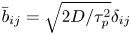 $\bar {b}_{ij} = \sqrt {2D/\tau _p^2} \delta _{ij}$, the dimensionless system of SDEs is given by
 \begin{gather} \mathrm{d}\boldsymbol{X}_{p,i} = St \boldsymbol{U}_{p,i}\,\mathrm{d}t, \end{gather}
 \begin{gather} \mathrm{d}\boldsymbol{U}_{p,i} = -\boldsymbol{U}_{p,i}\, \mathrm{d}t + \sqrt{2\left(Pe\,St \right)^{-1}}\, \mathrm{d}\boldsymbol{W}_t. \end{gather}
The corresponding Fokker–Planck equation is
 \begin{equation} \frac{\partial P(\boldsymbol{u},\boldsymbol{x};t|\boldsymbol{v},\boldsymbol{y},s)}{\partial t} + St \boldsymbol{\nabla}_{x} \boldsymbol{\cdot} \left(\boldsymbol{u}P\right) - \boldsymbol{\nabla}_{u} \boldsymbol{\cdot} (\boldsymbol{u}P) =(Pe\,St)^{-1}\Delta_{u}(P), \end{equation}
where the subscripts on the differential operators denote the coordinates of phase space that the derivatives are taken with respect to (position or velocity). Integration of (4.3) over the spatial coordinate yields the Fokker–Planck equation for the marginal velocity distribution. In one dimension, the equation is given by
 \begin{equation} \frac{\partial P(u;t|v,s)}{\partial t} - \frac{\partial \left(uP\right)}{\partial u} = \left(Pe\,St \right)^{-1}\frac{\partial^{2} P}{\partial u^{2}}. \end{equation}
Given an impulse initial condition for the particle velocity  $\delta (u-V_0)$, the solution to (4.4) may be obtained via Fourier transform and method of characteristics (Risken & Frank Reference Risken and Frank1996; Pope Reference Pope2000; Gardiner Reference Gardiner2009)
 \begin{equation} P(u;t) = \frac{1}{\sqrt{2{\rm \pi} (Pe\,St)^{-1} [1 - \exp(-2t)]}}\exp\left(-\frac{( u - V_0\exp(-t) )^2 }{2 (Pe\,St )^{-1}[1 - \exp(-2t)]}\right), \end{equation}
or  $\mathcal {N}[V_0\exp (-t), (Pe\,St )^{-1} [1 - \exp (-2t)]]$ for shorthand. We note that the restoring force in the Ornstein–Uhlenbeck process yields a bounded Gaussian distribution for velocity in the long time limit (
 $t \gg \tau _p$) with variance of
 $(Pe\,St )^{-1}$; as opposed to the unbounded variance for position obtained for the diffusion process in (3.10).
4.1. Fluctuating velocity (VL)
Applying the moment relations in § 3.2 to the Fokker–Planck equation given in (4.4) leads to
 \begin{gather} \frac{\textrm{d} \langle u \rangle}{\textrm{d} t} = - \langle u \rangle, \end{gather}
 \begin{gather} \frac{\textrm{d} \langle u^2 \rangle}{\textrm{d} t} = -2 \langle u^2 \rangle + 2\left(Pe\,St \right)^{-1}. \end{gather}
Equation (4.6b) is the one-dimensional analogue to the granular temperature balance obtained by Koch & Sangani (Reference Koch and Sangani1999) and Tenneti et al. (Reference Tenneti, Mehrabadi and Subramaniam2016). The first term on the right-hand side is the velocity dissipation, defined as  $\varGamma _{{vis}}=2R_{{diss}}(\phi )T/\tau _p$ by Koch & Sangani (Reference Koch and Sangani1999) and directly modelled from PR-DNS data by Tenneti et al. (Reference Tenneti, Mehrabadi and Subramaniam2016). Due to the non-dimensionalization here, the
 $1/\tau _p$ cancels on our dissipation term, and thus, the difference between our dissipation and that of Koch & Sangani (Reference Koch and Sangani1999) can be attributed to
 $R_{{diss}}(\phi )$. The second term is the source due to drag fluctuations, which VL models as a Wiener process increment. With a
 $V_0$ initial condition, integration of (4.6a) and (4.6b) yields
 \begin{gather} \langle u \rangle = V_0 \exp(-t),\end{gather}
 \begin{gather} \langle u^2 \rangle = (Pe\,St)^{-1} + (V_0^2 - (Pe\,St)^{-1} )\exp(-2t). \end{gather}
The time evolution of the velocity variance is then given by
 \begin{equation} \langle (u - \langle u \rangle )^2 \rangle = (Pe\,St)^{-1}[1 - \exp(-2t)], \end{equation}
which is again consistent with the known solution given in (4.5).
Following the arguments given at the end of § 3.2, (4.5) may be cast in dimensional form by replacing  $(Pe\,St )^{-1}$ with
 $D/(V_T^2\tau _p)$, multiplying by
 $V_T^2$ and setting
 $t = t/\tau _p$. We note that the diffusion tensor for an Ornstein–Uhlenbeck process is often set as
 $\sqrt {2\sigma _v^2/\tau _p}$, rather than
 $\sqrt {2D/\tau _p^2}$ as is done here; where
 $\sigma _v^2$ is a specified velocity variance. We set the diffusion tensor such that a canonical form is obtained for the dispersion solutions, thereby allowing straightforward comparison across different frameworks (PL, VL and FL). If one wishes to employ a diffusion tensor of
 $\sqrt {2\sigma _v^2/\tau _p}$ for the VL framework, then the variance solutions (4.8) and (4.12a) may be converted to dimensional form by substituting
 $\sigma _v^2\tau _p$ in place of
 $D$ – i.e. in dimensional variables, the steady granular temperature in (4.8) would be directly set by
 $\sigma _v^2$.
4.2. Dispersion (VL)
The spatial marginal distribution (integration of (4.3) over velocity space) leads to
 \begin{equation} \frac{\partial P(\boldsymbol{x};t|\boldsymbol{y},s)}{\partial t} + St \boldsymbol{\nabla}_{x} \boldsymbol{\cdot} (\langle u | x \rangle P) = 0, \end{equation}
where  $\langle u|x \rangle$ is the average velocity conditioned on position. Taking the first and second spatial moments of (4.9) leads to
 \begin{gather} \frac{\textrm{d} \langle x \rangle}{\textrm{d} t} = St \langle u \rangle, \end{gather}
 \begin{gather} \frac{\textrm{d} \langle x^2 \rangle}{\textrm{d} t} = 2 St \langle x \langle u | x \rangle \rangle, \end{gather}
 \begin{gather} \frac{\textrm{d} \langle (x - \langle x \rangle)^2 \rangle}{\textrm{d} t} \equiv 2 St (\langle x \langle u | x \rangle \rangle - \langle x \rangle \langle u \rangle) = 2 St \int_0^{s_2} K_{uu}(s_1,s_2) \, \mathrm{d}s_1, \end{gather}
where  $K_{uu}=Pe^{-1} \{\exp (-(s_2 - s_1)) - \exp (-(s_2 + s_1)) \}$ is the velocity autocovariance function. Obtaining the second equality in (4.10c) is non-trivial and the detailed derivation is given in appendix A.1. Integrating (4.10c), we arrive at the evolution equation for position variance.
An important simplification to the present derivation may be observed for the case of a constant velocity variance – i.e. if the particle velocity is initialized with a Maxwellian distribution  $\mathcal {N}[0, (Pe\,St )^{-1}]$ ((4.5) at steady state). For the Maxwellian initial condition, the velocity variance is independent of time and the autocovariance may be written in terms of a single time lag
 $K_{uu}(s_1) = (Pe\,St )^{-1} \exp (-s_1)$; leading to different dispersion behaviour at early times (see derivation in appendix A.2 and discussion in § 4.3). Evaluating the integral for mean position (4.10a) leads to
 \begin{equation} \langle x \rangle = V_0 St [1 - \exp(-t)], \end{equation}
while the integral for position variance (A 5) gives
 \begin{gather} \langle (x - \langle x \rangle)^2 \rangle = 2 St\,Pe^{-1} \left\{t - 2\mathbb{E}_1 + \frac{1}{2}\mathbb{E}_2\right\}, \end{gather}
 \begin{gather} \mathbb{E}_1 = [1 - \exp(-t)], \end{gather}
 \begin{gather} \mathbb{E}_2 = [1 - \exp(-2t)]. \end{gather}
4.3. Preliminary discussion
Comparing the position variance arising from PL and VL (Maxwellian and impulse initial condition), viz.
 \begin{gather} \langle (x - \langle x \rangle)^2 \rangle = 2 St\,Pe^{-1} t, \end{gather}
 \begin{gather} \langle (x - \langle x \rangle)^2 \rangle = 2 St\,Pe^{-1} \{ t - \mathbb{E}_1\}, \end{gather}
 \begin{gather} \langle (x - \langle x \rangle)^2 \rangle = 2 St\,Pe^{-1} \left\{ t - 2\mathbb{E}_1 + \frac{1}{2}\mathbb{E}_2\right\}, \end{gather}
demonstrates the canonical form prefaced in § 4.1. Namely, PL gives pure diffusion while VL gives diffusion in addition to exponential time scales  $\mathbb {E}_i$ that arise from the drag force and the initial condition. At sufficiently long times, VL dispersion converges to pure diffusion. If the particle velocities are initialized with the steady Maxwellian distribution in VL, then the velocity variance has no time dependence and the velocity autocovariance function depends upon a single time lag
 $s_1$. As a direct result, the integral in (A 5) simplifies and the classic ballistic–diffusive solution of Taylor (Reference Taylor1922) is recovered; see (4.13b). By contrast, if the particles are initialized with zero velocity, then the granular temperature evolves in time and additional time scales are introduced into the ballistic regime that act to suppress dispersion; see (4.13c). Thus, the solution in (4.13c) demonstrates the impact of a temporally evolving velocity variance on particle dispersion with the VL framework. Since ballistic dispersion terms scale with
 $\tau _p^2$, they are most significant for highly inertial particles.
The solutions given in (4.13b) and (4.13c) are first verified against numerical integration of (4.2a) and (4.2b) with  $St=5$ and
 $Pe=2$. Specifically, the analytical distribution
 $P(x;t) = \mathcal {N}[0,\sigma ^2]$, with
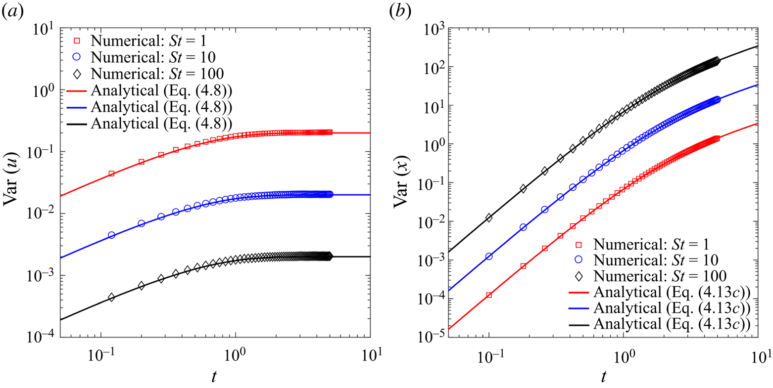
 $\sigma ^2$ given in (4.13a)–(4.13c) is compared to distributions obtained on the binned computational domain; see figure 1. Strong agreement is observed between the analytical solutions and numerical results for both the impulse (figure 1a,b) and Maxwellian (figure 1c,d) velocity conditions. Additionally, the ensemble averaged velocity variance and position variance, at
 $Pe=5$ and
 $St = 1, 10, 100$, are compared to (4.8) and (4.13c) in figure 2. As the Stokes number is reduced, particles behave more like fluid tracers and their velocity fluctuations undergo rapid relaxation, thereby yielding reduced dispersion. The classic ballistic
 $(t \leq 1)$ and diffusive
 $(t \geq 5)$ regimes may be seen in the dispersion curves in figure 2.
 $(a)$ Analytical and numerical predictions for velocity variance with the VL framework and an impulse velocity condition.
 $(b)$ Analytical and numerical predictions for position variance with the VL framework and an impulse velocity condition.
 $Pe=5$ for each Stokes number.

5. Force Langevin (FL)
As noted in § 1, force Langevin treatments are far less pervasive within the particle-laden flow literature; the works by Esteghamatian et al. (Reference Esteghamatian, Euzenat, Hammouti, Lance and Wachs2018) and Andrews et al. (Reference Andrews, Loezos and Sundaresan2005) being noted exceptions. Since the application of FL schemes has been empirical in nature, the velocity variance and dispersion resulting from such a framework has not been emphasized in the literature. While not a force Langevin, the fluctuating fluid velocity model of Pozorski & Apte (Reference Pozorski and Apte2009) has some interesting analogies to the FL scheme. Specifically, an additional SDE is introduced for the fluctuating fluid velocity which is commonly taken to follow an Ornstein–Uhlenbeck process. We consider a similar approach for the force Langevin, motivated by the Gaussian drag forces reported by PR–DNS studies. While we do not consider the task here, solutions obtained within this section for FL may be readily adapted to fluid VL schemes.
For the FL treatment we begin by splitting the total drag force into a mean and fluctuating component  $\boldsymbol {F}_{d,i} = \left \langle \boldsymbol {F}_{d}\right \rangle + \boldsymbol {F}^{\prime }_{d,i}$ (Esteghamatian et al. Reference Esteghamatian, Euzenat, Hammouti, Lance and Wachs2018). Random increments introduced on the particle force lead to
 \begin{gather} \mathrm{d}\boldsymbol{X}_{p,i} = \boldsymbol{U}_{p,i}\,\mathrm{d}t \end{gather}
 \begin{gather} \mathrm{d}\boldsymbol{U}_{p,i} = -\frac{1}{\tau_p} \boldsymbol{U}_{p,i}\,\mathrm{d}t + \frac{\boldsymbol{F}_{d,i}}{m_{p,i}}\,\mathrm{d}t, \end{gather}
 \begin{gather} \mathrm{d}\boldsymbol{F}_{d,i} = -\frac{1}{\tau_F} \boldsymbol{F}_{d,i}\,\mathrm{d}t + \hat{\boldsymbol{b}}\, \mathrm{d}\boldsymbol{W}_t, \end{gather}
where the  $(\cdot )^{\prime }$ notation is again omitted for readability. In order to keep the fluctuating force distribution bounded, a restorative component must be present in the force SDE. Similar to Pozorski & Apte (Reference Pozorski and Apte2009) and Esteghamatian et al. (Reference Esteghamatian, Euzenat, Hammouti, Lance and Wachs2018), we consider an Ornstein–Uhlenbeck process with relaxation time scale
 $\tau _F$. Setting the diffusion tensor as
 $\bar {b}_{ij} = \sqrt {2Dm_{p,i}^2/\tau _p^2 \tau _F^2} \delta _{ij}$, we arrive at a dimensionless form of
 \begin{gather} \mathrm{d}\boldsymbol{X}_{p,i} = St \boldsymbol{U}_{p,i}\,\mathrm{d}t, \end{gather}
 \begin{gather} \mathrm{d}\boldsymbol{U}_{p,i} = -\boldsymbol{U}_{p,i}\,\mathrm{d}t + \boldsymbol{F}_{d,i}\,\mathrm{d}t, \end{gather}
 \begin{gather} \mathrm{d}\boldsymbol{F}_{d,i} = -St_F \boldsymbol{F}_{d,i}\,\mathrm{d}t + \sqrt{2 St_F^2\left(Pe\,St \right)^{-1}}\,\mathrm{d}\boldsymbol{W}_t, \end{gather}
where  $St_F = \tau _p/\tau _F$ relates the Stokes response time to the integral time scale of the fluctuating drag force. For large fluctuating Stokes numbers
 $St_F$, the fluctuating drag forces have a short lifespan in comparison to the particle response time. Under these conditions, one would expect the FL treatment to be similar to the VL treatment, where the fluctuating drag force contains no memory; see (4.1b). In the opposite limit of small
 $St_F$, the fluctuating forces persist for time scales larger than the Stokes response time and significant departure from the VL treatment should be expected. The corresponding one-dimensional Fokker–Planck equation is given by
 \begin{equation} \frac{\partial P}{\partial t} + St \frac{\partial }{\partial x} (uP) + \frac{\partial }{\partial u} [(\,f - u)P] - St_F \frac{\partial }{\partial f} (\,f P)= St_F^2(Pe\,St)^{-1} \frac{\partial^{2} P}{\partial {f}^{2}}. \end{equation}
Details derived for the Ornstein–Uhlenbeck process in § 4 ((4.6a)–(4.8)) may be directly applied to the fluctuating force – i.e. a mean of  $f_0\exp (-St_F t)$ and variance of
 $St_F(Pe\,St )^{-1}[1 - \exp (-2St_F t)]$.
In the limit of stationary particle assemblies, previous works have shown that a drag force distribution with characteristic variance will be present; see cited works in § 1. For this reason, we take the fluctuating force to be fully developed  $\mathcal {N}[0,St_F(Pe\,St )^{-1}]$ and do not consider the temporal growth of its variance. Thus, in the present derivation, the fluctuating force distribution is stationary with a constant variance and relaxation time. In general, FL is not restricted to a constant variance or relaxation time, and previous results with particle-resolved simulations suggest that these parameters will vary within a general multiphase flow (Koch & Sangani Reference Koch and Sangani1999; Huang et al. Reference Huang, Wang, Zhou and Li2017; Esteghamatian et al. Reference Esteghamatian, Euzenat, Hammouti, Lance and Wachs2018). Connections between the solutions derived here and PR–DNS are made in § 7, with emphasis being given to how the model coefficients may be informed.
For the sake of completeness, we note that the diffusion tensor has again been set to yield the canonical form for dispersion. If the diffusion tensor is set in the manner discussed at the end of § 4.1 $\sqrt {2\sigma _F^2/ \tau _F}$, then
 $\sigma _F^2$ characterizes the steady variance in fluctuating force. For this case, the solutions derived in this section may be cast in dimensional form by replacing
 $D$ with
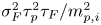 $\sigma _F^2\tau _p^2\tau _F/m_{p,i}^2$.
5.1. Fluctuating velocity (FL)
Integrating (5.3) over the spatial  $(x)$ and fluctuating force
 $(\,f)$ coordinates allows the marginal velocity distribution to be obtained
 \begin{equation} \frac{\partial P(u;t|v,s)}{\partial t} + \frac{\partial }{\partial u} [(\langle\, f|u\rangle - u)P] = 0. \end{equation}
The first two moments of (5.4) are given by
 \begin{gather} \frac{\textrm{d} \langle u \rangle}{\textrm{d} t} = - \langle u \rangle + \langle\langle\, f|u\rangle\rangle, \end{gather}
 \begin{gather} \frac{\textrm{d} \langle u^2 \rangle}{\textrm{d} t} = -2 \langle u^2 \rangle + 2\langle u\langle\, f|u\rangle\rangle. \end{gather}
Comparing the granular temperature balance with FL (5.5b) to VL (4.6b) shows that the functional form is unaltered but the source term is described by the force–velocity covariance with FL. This is a direct result of modelling the force statistics via FL as well as the substitution of the instantaneous particle velocity into Stokes drag. Since the fluctuating force is defined to be stationary with variance 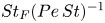 $St_F(Pe\,St )^{-1}$, the unconditional mean of force
 $\langle \langle\, f|u \rangle \rangle$ is zero, leading to zero mean velocity
 $\langle u \rangle$. We quickly recognize that
 $\langle u\langle\, f|u \rangle \rangle$ must be handled via Lagrangian variables in a similar manner to
 $\langle x \langle u | x \rangle \rangle$ in § 4.2. Starting with Newton's second law in dimensionless form
 \begin{equation} \frac{\textrm{d} U_{p,i}}{\textrm{d} t} = -U_{p,i} + F_{p,i}, \end{equation}
the particle velocity with time is given by
 \begin{equation} U_{p,i}(t) = \exp(-t) \int_0^t \exp(t^{\prime}) F_{p,i}(t^{\prime}) \, \mathrm{d}t^{\prime}, \end{equation}
leading to
 \begin{equation} \langle u\langle\, f|u\rangle\rangle = \exp(-t) \int_0^t \exp(t^{\prime}) \langle F_{p,i}(t^{\prime}) F_{p,i}(t) \rangle \, \mathrm{d}t^{\prime}. \end{equation}
Since the fluctuating force is fully developed, the two-time Lagrangian force correlation  $\left \langle F_{p,i}(t^{\prime })F_{p,i}(t) \right \rangle$ only depends upon a single time lag
 $K_{uu}(s_1) = St_F (Pe\,St )^{-1}$
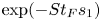 $\exp (-St_F s_1)$;
 $s_1 = t - t^{\prime }$. Therefore, the source term in (5.5b) follows
 \begin{equation} \langle u\langle\, f|u\rangle\rangle = St_F(Pe\,St )^{-1}\exp(-t) \int_0^t \exp(t^{\prime})\exp(-St_F(t-t^{\prime})) \, \mathrm{d}t^{\prime}. \end{equation}
Integrating (5.9), we arrive at
 \begin{equation} \langle u\langle\, f|u\rangle\rangle = (Pe\,St )^{-1} \frac{St_F}{St_F + 1} [1 - \exp(-(St_F + 1) t) ]. \end{equation}
Substituting (5.10) into (5.5b) allows an integrating factor solution for  $\langle u^2 \rangle$ to be found
 \begin{gather} \langle u^2 \rangle = 2 (Pe\,St)^{-1} \frac{St_F}{St_F + 1} \left\{ \frac{1}{2} \mathbb{E}_2 + \frac{1}{St_F - 1} (\mathbb{E}_2 - \mathbb{E}_3 ) \right\}, \end{gather}
 \begin{gather} \mathbb{E}_3 = [ 1 - \exp(-(St_F + 1) t)]. \end{gather}
For the special case that  $St_F = 1$ (
 $\tau _F = \tau _p$), the integrating factor for (5.5b) exactly offsets the exponential term in (5.10) and a simplified solution is obtained
 \begin{equation} \langle u^2 \rangle = (Pe\,St)^{-1} \left\{ \frac{1}{2} \mathbb{E}_2 - t\exp(-2t) \right\}. \end{equation}
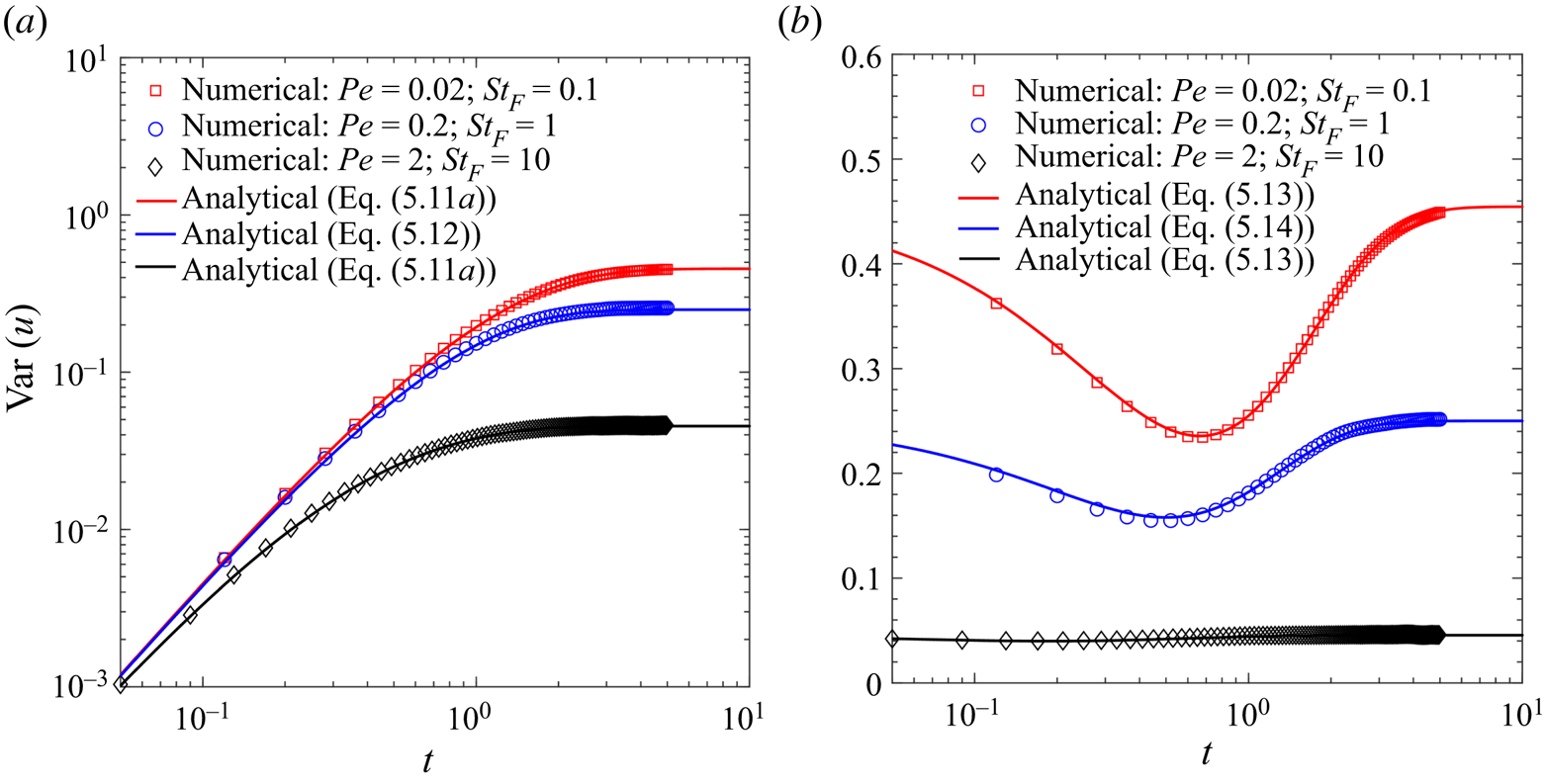
Granular temperatures computed from simulations with the FL scheme ((5.2a)–(5.2c)) are in excellent agreement with (5.11a)–(5.12); see figure 3(a). In figure 3(a) the Stokes number is held fixed while the fluctuating Stokes number and Péclet number are varied. For demonstration purposes, the Péclet numbers are chosen such that the force variance is conserved in all three simulations, thereby allowing the effect of the force memory,  $St_F$, to be probed. Reducing
 $St_F$, at a fixed force variance, causes the force fluctuations to decay at a slower rate and ultimately giving rise to enhanced granular temperatures. Therefore, fluctuating drag forces with significant inertia are characterized by small
 $St_F$. It is important to note that the VL scheme inherently assumes that the fluctuating drag force is non-inertial, just as the PL scheme assumes the particles themselves are non-inertial. This hierarchy further motivates the Stokes number analogy employed for the fluctuating force and allows a connection to be drawn to the VL scheme. Specifically, FL predicts larger granular temperatures as the fluctuating forces become more inertial, smaller
 $St_F$, just as the VL scheme predicts greater dispersion as the particles become more inertial, larger
 $St$.
 $(a)$ Analytical and numerical prediction for transient growth in the velocity variance with the FL framework and a
 $\delta (u)$ initial condition.
 $(b)$ Analytical and numerical predictions for the same system but with particle velocities initialized as a Maxwellian. In all cases,
 $St=10$.

It is important to note that the solution obtained in (5.11a) converges to a steady velocity variance of  $\langle u^2 \rangle _{\infty } = (Pe\,St )^{-1} St_F /(St_F + 1)$. However, the FL framework yields a time dependent granular temperature even if the system is initialized with the steady velocity variance. By contrast, the VL framework yields a constant granular temperature if the system is initialized with the steady velocity variance; see (4.8) with an initial condition of
 $(Pe\,St )^{-1}$. To emphasize this point, we consider imposing an IC of
 $\langle u^2 \rangle _{\infty }$ when solving (5.5b) to obtain
 \begin{equation} \langle u^2 \rangle = 2 \left(Pe\,St \right)^{-1} \frac{St_F}{St_F + 1} \left\{ \frac{1}{2} - \frac{1}{St_F - 1} (\mathbb{E}_2 - \mathbb{E}_3) \right\}, \end{equation}
and for the case  $St_F=1$
 \begin{equation} \langle u^2 \rangle = (Pe\,St)^{-1} \left\{ \frac{1}{2} - t\exp(-2t) \right\}. \end{equation}
Comparing (5.13) to numerical results shows the time dependence of the granular temperature; see figure 3(b). At long times, the system converges to a velocity variance of  $(Pe\,St )^{-1} St_F /(St_F + 1)$. However, an initial reduction in granular temperature is observed, due to the
 $\mathbb {E}_3$ time scale (force–velocity covariance), and the recovery time depends upon the fluctuating Stokes number (competition between
 $\mathbb {E}_3$ and
 $\mathbb {E}_2$ terms).
The aforementioned results may be physically understood by recognizing that the Maxwellian distributions employed for the fluctuating force and particle velocity are sampled independently when the system is initialized. Therefore, the fluctuating forces, which drive the granular temperature, are not correlated with the particle velocities when the system begins evolving. Since the force–velocity correlations develop over time scales associated with the fluctuating Stokes number, the effect of the initial force condition persists longer as  $St_F$ is decreased and leads to the accentuated dips in figure 3(b). We stress that the initial reduction in granular temperature, due to force–velocity covariances, is indeed physical and was observed in the PR–DNS simulations of Tenneti et al. (Reference Tenneti, Mehrabadi and Subramaniam2016) with freely evolving particles (see green curve in figure 5a of Tenneti et al. Reference Tenneti, Mehrabadi and Subramaniam2016). As we increase the fluctuating Stokes number, dips in granular temperature are less prominent; and at sufficiently large
 $St_F$, the granular temperature remains constant. This behaviour is consistent with what would be obtained by a VL framework, which treats the fluctuating forces as non-inertial. In summary, the fluctuating Stokes number characterizes the inertia of the fluctuating drag force and gauges the departure of FL from VL. The potential dependencies of
 $St_F$ and connections with various types of flows are discussed in greater detail in § 6.
5.2. Dispersion (FL)
Integrating (5.3) over the fluctuating force  $f$ and velocity
 $u$ coordinates allows the marginal spatial distribution to be obtained
 \begin{equation} \frac{\partial P(x;t|y,s)}{\partial t} + St \frac{\partial }{\partial x} [ \langle u|x \rangle P ] = 0. \end{equation}
The first two moments of (5.15) are given by
 \begin{gather} \frac{\textrm{d} \langle x \rangle}{\textrm{d} t} = St \langle\langle u|x\rangle\rangle, \end{gather}
 \begin{gather} \frac{\textrm{d} \langle x^2 \rangle}{\textrm{d} t} = 2St \langle x\langle u|x\rangle\rangle. \end{gather}
The unconditional velocity  $\langle \langle u|x\rangle \rangle$ was shown to be zero in § 5.1 (stationary distribution for
 $f$), and thus, the mean position will also be zero. The
 $\left \langle x\left \langle u|x\right \rangle \right \rangle$ term is addressed in the same manner as appendix A.1 and the details are given in appendix A.3. Additionally, for the sake of completeness, the velocity autocovariance function for a fully developed velocity distribution is derived in appendix A.4. Integration of the velocity autocovariance function gives a closed-form solution for position variance
 \begin{equation} \langle x^2\rangle = 2 St\,Pe^{-1}\{ t - C_1 \mathbb{E}_1 + C_2 \mathbb{E}_2 - C_3 \mathbb{E}_3 + C_4 \mathbb{E}_4\}, \end{equation}
where  $\mathbb {E}_4 = [1 - \exp (-St_F t ) ]$ and the constants
 $(C_i)$ are given by
 \begin{gather} C_1 = \frac{2 St_F - 1}{St_F - 1}, \end{gather}
 \begin{gather} C_2 = \frac{St_F}{2(St_F - 1)}, \end{gather}
 \begin{gather} C_3 = \frac{1}{(St_F + 1)(St_F - 1)}, \end{gather}
 \begin{gather} C_4 = \frac{1}{St_F(St_F-1)}. \end{gather}
Repeating the process for  $St_F=1$ leads to
 \begin{equation} \langle x^2\rangle = 2 St\,Pe^{-1} \left\{ t - 3 \mathbb{E}_1 + \frac{3}{4} \mathbb{E}_2 + t \exp(-t) - \frac{1}{2} t \exp(-2t) \right\}. \end{equation}
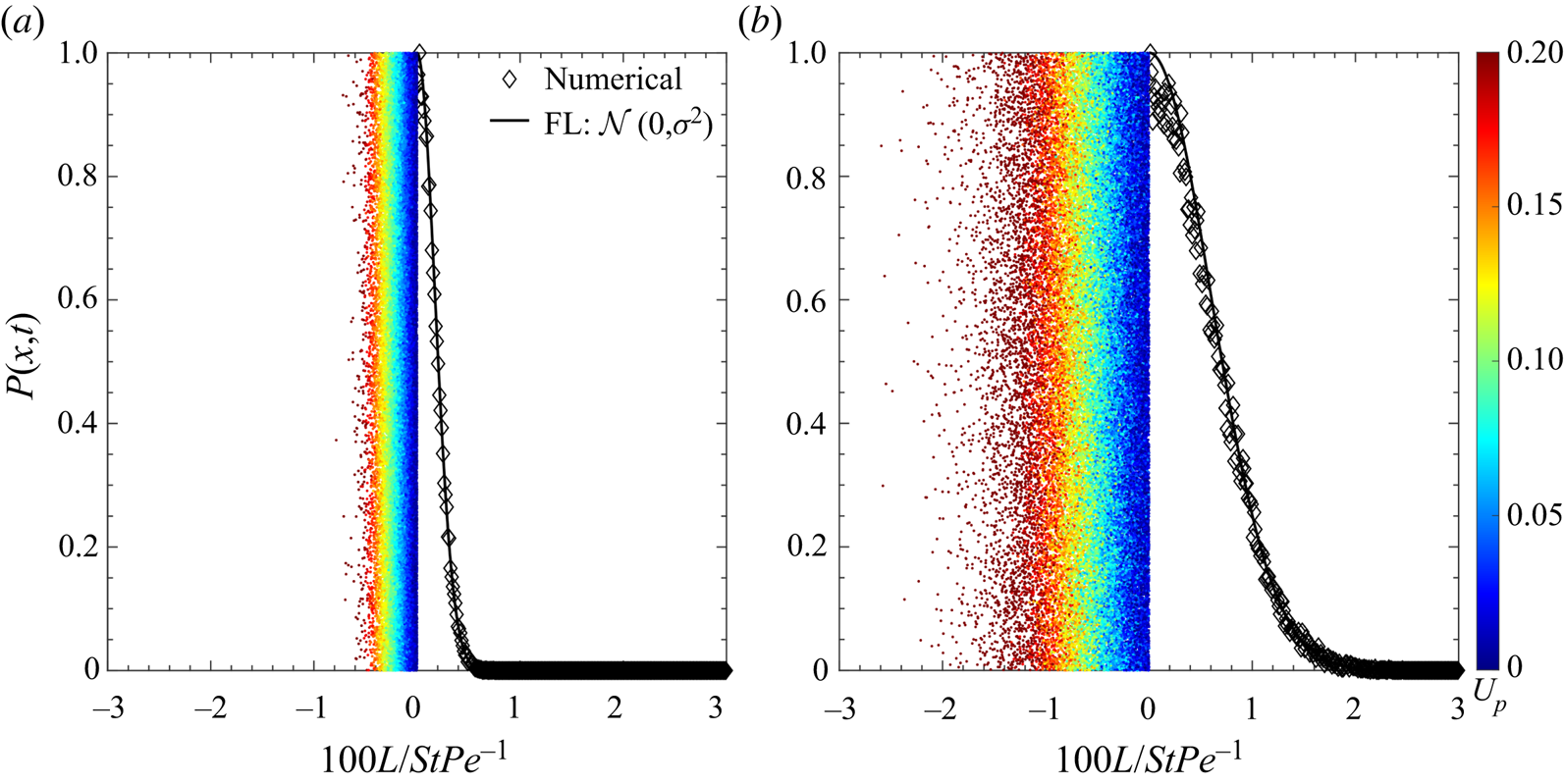
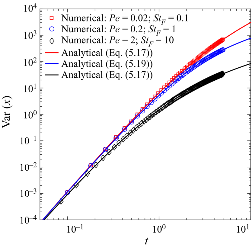
The analytical solution for dispersion, Gaussian distribution  $P(x;t) = \mathcal {N}[0,\sigma ^2]$ with the variance specified by (5.17), is in strong agreement with numerical results; see figure 4. The conditions in figure 4 are given by:
 $St=100$,
 $Pe=0.1$, and
 $St_F=0.3$. Ensemble averaging of the position variances, at the same conditions considered in figure 3 (constant force variance), yields the curves in figure 5. Examination of figures 5 and 3 shows that, for a constant force variance, smaller
 $St_F$ lead to larger granular temperature and greater dispersion. Furthermore, it becomes clear that the force variance and the relaxation time scale allow the FL framework to control the granular temperature and dispersion. By contrast, the VL framework with a mean drag closure only allows for control of the granular temperature (dispersion is a result of the specified velocity variance), and the PL framework only allows for control of the long time diffusion behaviour.
(a,b) Analytical and numerical predictions for particle dispersion with the FL framework. An impulse velocity condition was utilized in all cases and the conditions are given by  $St = 100$,
 $Pe = 0.1$,
 $St_F=0.3$. Particles (left half of images) are coloured by the magnitude of their velocity in the
 $x$-direction.
 $(a)\,\, t = 0.500, (b)\,\, t = 1.000.$

Analytical and numerical predictions for dispersion with the FL framework. An impulse velocity condition was utilized in all cases and  $St=10$.

6. Discussion
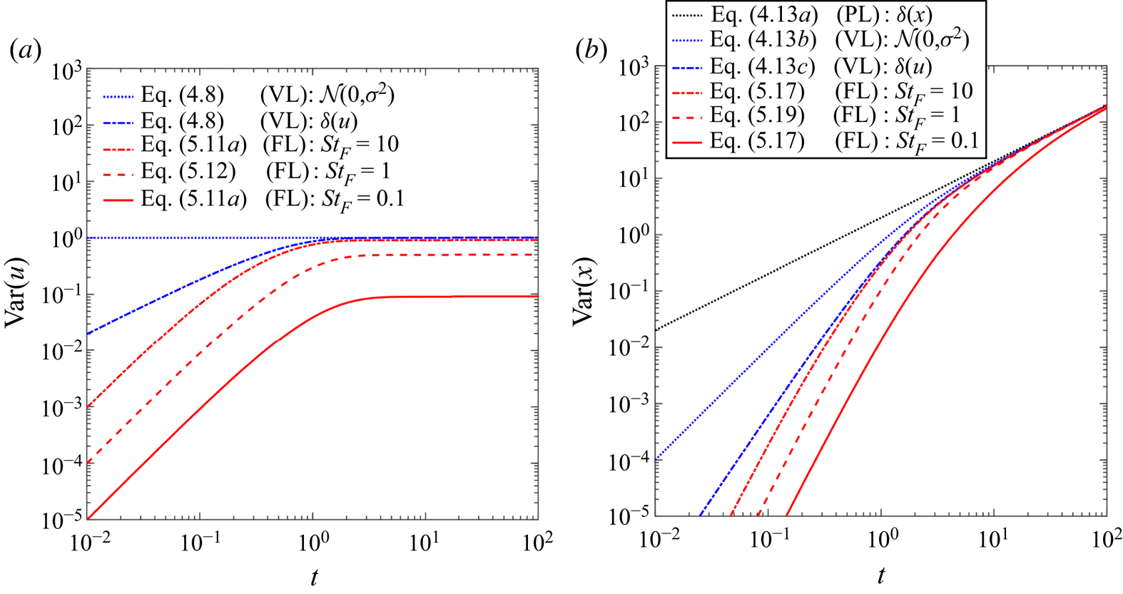
Comparing dispersion with FL (5.17), VL (4.12a) and PL (3.10) illustrates that the functional form remains unaltered (long time diffusion and short time exponential expansion); see figure 6. From a physical point of view, the curves in figure 6 may be interpreted as the velocity variance required by a method to obtain a specified diffusion coefficient. We note that velocity variance is an input to VL and an output of FL. Therefore, the FL framework allows for the most complex behaviour since it may attain a desired level of dispersion at different granular temperatures. To further demonstrate this, we consider the behaviour of the FL scheme at large and small  $St_F=\tau _p/\tau _F$. As
 $St_F$ increases, the fluctuating drag becomes less inertial (short force memory) and the treatment employed by the VL framework is approached. Considering the limit
 $St_F \rightarrow \infty$ on (5.18a)–(5.18d), we formally show convergence of FL dispersion to VL dispersion (4.13c). Similarly, the same limit may be considered on (5.11a) to show convergence of FL granular temperature to VL granular temperature (4.8). As
 $St_F$ is reduced, FL schemes predict larger velocity variances (figure 3a) and greater dispersion (figure 5), due to the persistence of force–velocity covariances. Therefore, FL schemes are more appropriate for small fluctuating Stokes numbers since they account for the inertia of the drag force fluctuations.
 $(a)$ Granular temperature obtained with VL and FL,
 $(b)$ dispersion behaviour obtained with PL, VL and FL with
 $St=1$ and
 $Pe=1$.

It is not known a priori how the fluctuating Stokes number will behave in a general particle-laden flow. However, some qualitative expectations are instructive. For flows with elevated granular temperature, the particle structure rapidly rearranges and the interactions between particles and fluid wakes may be short lived (large  $St_F$). By contrast, at lower granular temperature, particles may reside in the fluid wake of their neighbours for appreciable time (small
 $St_F$). Similarly, Koch & Sangani (Reference Koch and Sangani1999) considered the role of the force autocorrelation as a source to granular temperature and suggest that significant changes to the particle structure will occur over time scales of
 $d_p/T^{1/2}$. For the force time scale of Koch & Sangani (Reference Koch and Sangani1999), a general multiphase flow may experience a range of fluctuating Stokes numbers (local and time varying) where regions with high granular temperature are appropriately approximated by a VL scheme but regions of low granular temperature could require a FL scheme.
Practically speaking, it is desirable to obtain the correct granular temperature and dispersion in an EL framework. Therefore, we consider the position and velocity variance obtained with VL, FL, the model of Tenneti et al. (Reference Tenneti, Mehrabadi and Subramaniam2016) and adapting the theory of Koch & Sangani (Reference Koch and Sangani1999) to VL. Details regarding the implementation of Koch & Sangani (Reference Koch and Sangani1999) are given in appendix C.1. We specify the steady velocity variance  $\sigma _v^2$ in VL with the granular temperature correlation of Tenneti et al. (Reference Tenneti, Mehrabadi and Subramaniam2016). Therefore, VL and the model of Tenneti et al. (Reference Tenneti, Mehrabadi and Subramaniam2016) must obtain the same steady velocity variance regardless of differences in their velocity dissipation time scale
 $\gamma$ versus
 $1/\tau _p$. However, differences in the velocity dissipation will affect the resulting dispersion. The FL solutions obtained here require that the force time scale
 $\tau _F$ and force variance
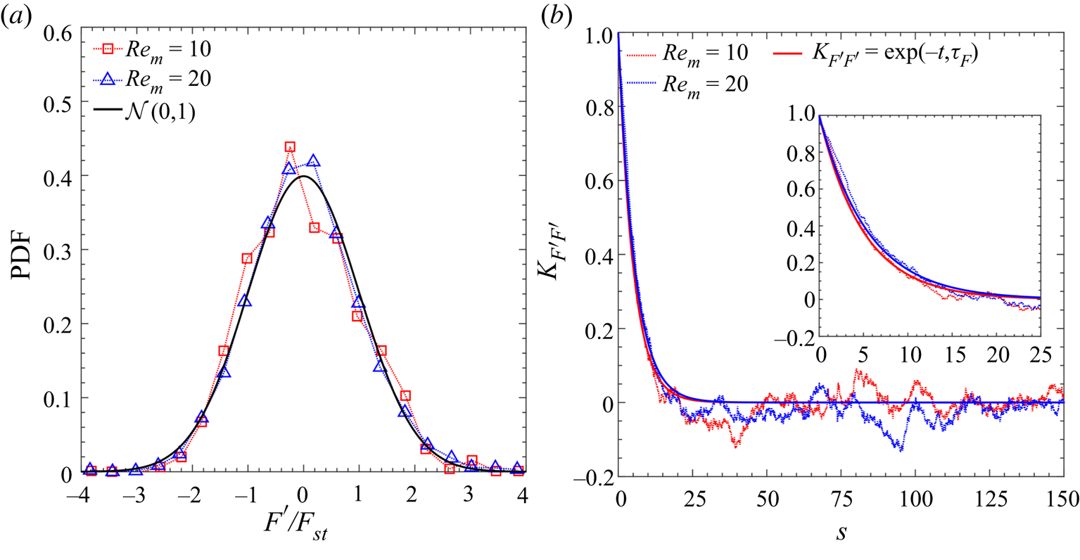
 $\sigma _F^2$ be specified. These terms were extracted from the PR–DNS of Tavanashad et al. (Reference Tavanashad, Passalacqua, Fox and Subramaniam2019) in the direction of mean slip; see discussion in appendix B. The normalized drag fluctuations are well approximated by a Gaussian distribution with variance
 $\sigma _F^2 / F_{st}^2 = 1$, where
 $F_{st}^2 = (3 {\rm \pi} \mathrm {\mu } d_p (1-\phi ) V_T)^2$ represents Stokes drag. The particle diameter
 $d_p = 500 \times 10^{-6} \ \mathrm {m}$, particle density
 $\rho _p = 100 \ \mathrm {kg}\,\mathrm {m}^{-3}$, fluid viscosity
 $\mathrm {\mu } = 1.0 \times 10^{-5} \ \mathrm {Pa}\,\mathrm {s}$, fluid density
 $\rho _f = 1.0 \ \mathrm {kg}\,\mathrm {m}^{-3}$ and solids volume fraction
 $\phi = 0.1$ were held fixed in all cases. The force time scales
 $\tau _F$ are normalized by
 $d_p/V_T$, where
 $V_T$ is determined by the mean Reynolds number
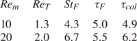
 $Re_m = 10, \ 20$. Other relevant properties are summarized in table 1.
Parameters for comparison of FL and VL. The force time scale  $\tau _F$ and mean-free time scale
 $\tau _{col}$ are non-dimensionalized by
 $d_p/V_T$, where
 $V_T$ is the slip velocity specified by the Reynolds number. All cases correspond to
 $\rho _p/\rho _f =100$ and
 $\phi =0.1$.

Since FL predicts the velocity variance, rather than taking it as an input, care must be taken with this method. At the conditions considered here, Stokes flow will not adequately describe the dissipation of velocity fluctuations. To account for finite  $Re_m$ and
 $\phi$, we employ the drag correlation of Tenneti et al. (Reference Tenneti, Garg and Subramaniam2011) to define an effective dissipation time scale
 $\tau _{p,{eff}}$ for FL; see appendix C.2. The selected drag correlation is motivated by the discussion in the second paragraph of § 4 where it was noted that particle velocity fluctuations inherit the mean drag time scale when an instantaneous particle velocity is utilized. Therefore, the treatment is intended to be consistent with an EL method that utilizes the drag correlation of Tenneti et al. (Reference Tenneti, Garg and Subramaniam2011) and an instantaneous particle velocity. We note that a similar approach is utilized for the adaptation of Koch & Sangani (Reference Koch and Sangani1999), where
 $R_{{diss}}(\phi )$ is utilized to approximate
 $\tau _{p,{eff}}$. Therefore, the fluctuating Stokes numbers reported in table 1 are computed as
 $St_F = \tau _{p,{eff}}/\tau _F$. Additionally, the PR–DNS simulations exhibit anisotropy in the velocity variance. Specifically, the velocity variance in the mean slip direction is
 ${\sim }2{\times }$ that in the transverse directions (Tavanashad et al. Reference Tavanashad, Passalacqua, Fox and Subramaniam2019). Since FL solutions only use statistics from the mean slip direction, we account for anisotropy by taking the granular temperature to be 2/3 the predicted velocity variance.
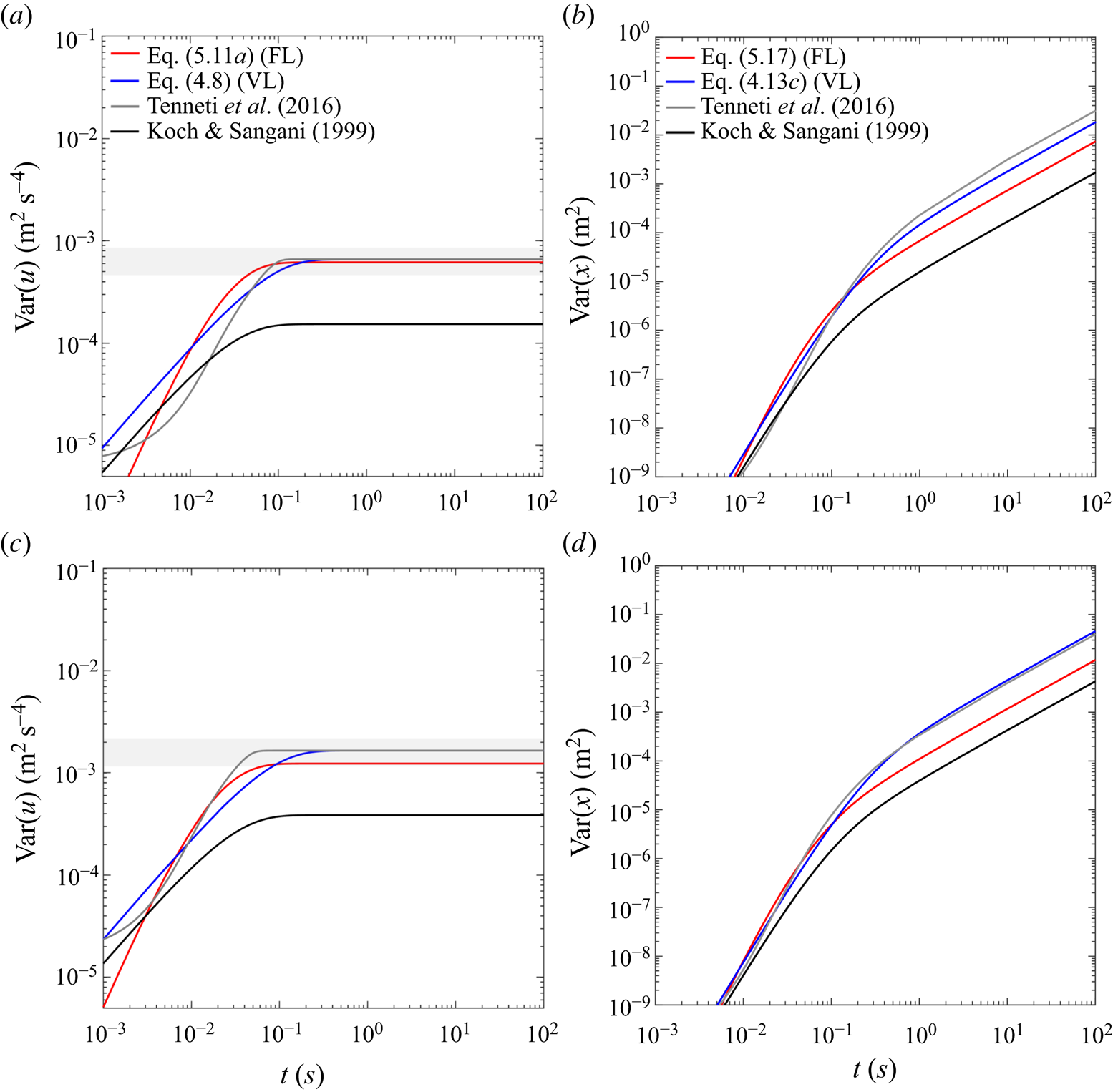
The dimensional granular temperature and dispersion curves are visualized in figure 7. The theory of Koch & Sangani (Reference Koch and Sangani1999) is obtained for Stokes flow and yields lower granular temperatures than the other methods. As a direct consequence of the smaller velocity variance, dispersion obtained with Koch & Sangani (Reference Koch and Sangani1999) is also the lowest. While VL and the model of Tenneti et al. (Reference Tenneti, Mehrabadi and Subramaniam2016) must obtain the same steady granular temperature, the dispersion resulting from each method need not match. The dispersion curves in figure 7(b,d) for VL and Tenneti et al. (Reference Tenneti, Mehrabadi and Subramaniam2016) imply that  $\gamma$ must be similar to or less than
 $1/\tau _p$ at the conditions considered here. Thus, in the model of Tenneti et al. (Reference Tenneti, Mehrabadi and Subramaniam2016), velocity fluctuations are dissipated much slower than the mean drag correlation of Tenneti et al. (Reference Tenneti, Garg and Subramaniam2011) or the
 $R_{{diss}}(\phi )$ closure of Koch & Sangani (Reference Koch and Sangani1999). The slow dissipation of velocity fluctuations by Tenneti et al. (Reference Tenneti, Mehrabadi and Subramaniam2016) results in larger dispersion.
The granular temperature behaviour obtained at  $(a)$
 $Re_m=10$ and
 $(c)$
 $Re_m=20$ with VL, FL, the model of Tenneti et al. (Reference Tenneti, Mehrabadi and Subramaniam2016) and adapting the closures of Koch & Sangani (Reference Koch and Sangani1999) to VL. Dispersion curves resulting from the aforementioned models at
 $(b)$
 $Re_m=10$ and
 $(d)$
 $Re_m=20$ . The grey regions correspond to
 ${\pm }30\,\%$ about the granular temperature correlation of Tenneti et al. (Reference Tenneti, Mehrabadi and Subramaniam2016).

Accounting for anisotropy, as well as  $Re_m$ and
 $\phi$ effects, in FL yields outputs for granular temperature that agree with the correlation of Tenneti et al. (Reference Tenneti, Mehrabadi and Subramaniam2016). Dispersion with FL is significantly lower than that obtained with VL or Tenneti et al. (Reference Tenneti, Mehrabadi and Subramaniam2016). This behaviour can be attributed to the rapid dissipation of velocity fluctuations in FL with the correlation of Tenneti et al. (Reference Tenneti, Garg and Subramaniam2011). Namely, the
 $St_F$ values are not sufficiently large that the velocity dissipation
 $\tau _{p,{eff}}$ and force dissipation
 $\tau _F$ exhibit a complete separation of time scales. Therefore, FL, to some degree, overcomes the increase in velocity dissipation with finite memory forces to obtain the same granular temperature as VL and Tenneti et al. (Reference Tenneti, Mehrabadi and Subramaniam2016). It is worth noting that a VL model could be constructed with the
 $\tau _{p,{eff}}$ time scale utilized for FL. Doing so would emphasize the force memory effects on dispersion, since both VL and FL would obtain the same granular temperature. Completing this task, we observe a dispersion coefficient with FL that is
 ${\sim }15\,\%$ larger than VL.
7. Model development for Euler–Lagrange methods
In general, FL requires closure of two model parameters: (i) the drift vector (integral time scale of fluctuating force;  $\tau _F$) and (ii) the diffusion tensor (force variances;
 $\sigma _F^2$). Examining the fluid–particle force statistics within PR–DNS of freely evolving particles allows both parameters to be probed. The relaxation time scale(s) may be examined via the two-time force autocovariance; see appendix B here and equation (28) in Esteghamatian et al. (Reference Esteghamatian, Euzenat, Hammouti, Lance and Wachs2018). Preliminary examinations of the force autocovariance have been made by Esteghamatian et al. (Reference Esteghamatian, Bernard, Lance, Hammouti and Wachs2017), but correlations for this quantity are not readily available in the literature. Similarly, the drag force variance has been reported in a variety of PR–DNS works (Koch & Sangani Reference Koch and Sangani1999; Wylie et al. Reference Wylie, Koch and Ladd2003; Akiki et al. Reference Akiki, Jackson and Balachandar2016; Huang et al. Reference Huang, Wang, Zhou and Li2017), but again, correlations for this quantity are not well established. Since force time scales extracted from PR–DNS may lead to small fluctuating Stokes numbers, where differences between FL and VL occur, it appears that the FL framework may have a significant impact on certain multiphase flows. Therefore, well characterized inputs to the FL framework, obtained from statistical analysis of the drag forces present in freely evolving suspensions, would be useful.
There are a variety of means by which the present analysis may be extended. For large Stokes numbers, Koch & Sangani (Reference Koch and Sangani1999) approximate the time scale for the drag force with the mean-free time between successive collisions (Chapman, Cowling & Burnett Reference Chapman, Cowling and Burnett1970)
 \begin{equation} \tau_{col} = \frac{d_p}{24 \phi \chi} \sqrt{\frac{{\rm \pi}}{T}}, \end{equation}
where  $\chi$ is the radial distribution function (RDF) at contact. The mean-free time
 $\tau _{col}$, computed with the correlation of Tenneti et al. (Reference Tenneti, Mehrabadi and Subramaniam2016) and the RDF of Ma & Ahmadi (Reference Ma and Ahmadi1988), is observed to be in good agreement with the
 $\tau _F$ time scales extracted from PR–DNS; see table 1. It is worth noting that
 $\tau _{col}$ is
 ${\sim }13\,\%$ larger than
 $\tau _F$ for the
 $Re_m=20$ case and actually improves agreement between FL theory and the correlation of Tenneti et al. (Reference Tenneti, Mehrabadi and Subramaniam2016). Therefore, taking
 $\tau _{col} \approx \tau _F$ and correlating the force variances
 $\sigma _F^2$ in static particle assemblies may constitute an appropriate model for large Stokes numbers. Physically, larger granular temperatures will lead to rapid alteration of particle structuring and shorter force memories. While the data in table 1 only constitute two points, values of
 $St_F$ are observed to increase with increasing
 $Re_T$. Informing the force time scale with the granular temperature would provide valuable connections between the velocity and force equations, which are presently one-way coupled. Since the steady, fluid-mediated, granular temperature is defined by the
 $(\rho _f/\rho _p, \ \phi , \ Re_m )$ triple point (Tenneti et al. Reference Tenneti, Mehrabadi and Subramaniam2016), an implicit relation between the flow conditions and FL inputs is expected. Under this modelling paradigm, space–time locality should also be explored since variation in the flow conditions will lead to variation in the FL inputs. Additionally, sub-grid, pseudo-turbulent fluid velocity fluctuations (Mehrabadi et al. Reference Mehrabadi, Tenneti, Garg and Subramaniam2015) may prove useful for informing the drag variance. Specifically, the use of rotation matrices, as in Peng et al. (Reference Peng, Kong, Zhou, Sun, Passalacqua, Subramaniam and Fox2019), may allow for anisotropic behaviour. For this case, fluctuating forces in a body-fixed coordinate system aligned with the slip velocity would be constructed and then rotated back to the laboratory reference frame. Such a framework could account for stochastic forces in the direction of mean slip, as well as the transverse directions.
8. Conclusions
In the context of application to EL frameworks, three stochastic methods for neighbour-induced drag force fluctuations were discussed. Stochastic methods correspond to Langevin equations for the particle position, particle velocity and the fluctuating drag force. Analytical solutions for the dispersion and velocity variance were derived under the assumptions of Stokes drag and collisionless particles. Dispersion and velocity variance solutions were verified against numerical results on a doubly periodic rectangular grid. The solutions derived herein demonstrate that the system of Langevin equations (PL, VL, FL) form a hierarchy in terms of the physics they are capable of resolving. Specifically, PL only allows for control of the particle dispersion and does not provide a means for controlling granular temperature. VL allows for control of the granular temperature, but the dispersion is a consequence of the dissipation time scale for velocity fluctuations. FL allows for control of the granular temperature and dispersion, but requires the statistics of the neighbour-induced fluctuating drag force be specified (variance and integral time scale), which are not classically correlated quantities. Formal convergence of the FL scheme to the VL scheme is shown in the limit of large fluctuating Stokes numbers  $St_F$ – i.e. the integral time scale of the fluctuating force is much smaller than the Stokes response time. In the opposite limit, the fluctuating drag forces have non-negligible memory and the FL scheme predicts greater dispersion than VL at the same granular temperature. Quantifying inputs to the FL framework is most appropriately addressed via particle-resolved direct numerical simulations with freely evolving particles. In this spirit, connections between the force variance and the pseudo-turbulent Reynolds stresses may prove valuable.
In contrast to deterministic approaches that attempt to map the effect of neighbour-induced velocity fluctuations directly to each particle (Akiki et al. Reference Akiki, Jackson and Balachandar2017), the present method is formulated to capture such effects on the statistics of an assembly of particles (particle velocity variance and mean displacement). It should be noted that such an approach is not appropriate for cases in which precise details of individual particle trajectories are needed, especially for small particle assemblies like in the classic example of drafting, kissing and tumbling. The stochastic framework developed here acts as the foundation for improved EL methods where the neighbour-induced flow, changing over length scales comparable or smaller than the particle diameter, is not resolved. Near-future work will consider quantification of FL inputs as well as implementation of the FL method within an EL framework. Additionally, FL theory leads to fluid-mediated source and sink terms in the granular temperature balance. A long term goal of the present work is to develop closures for these sink and source terms for use in EE frameworks.
Acknowledgements
This material is based upon work supported by the National Science Foundation under grant no. CBET-1904742 and grant no. CBET-1438143.
Declaration of interests
The authors report no conflict of interest.
Appendix A. Supporting derivations
A.1. Velocity Langevin:  $\delta (u)$

The moments in (4.10a)–(4.10c) are taken over all of phase space (position and velocity coordinates) and thus should be equal to ensemble averaging of the Lagrangian particles. Therefore, we seek to relate the unconditional mean of position and velocity to two-time Lagrangian statistics. Utilizing the fact that particle position is the integral of velocity  $x = St \int u$, we obtain
 \begin{gather} \langle x \langle u | x \rangle \rangle \equiv \left\langle St \int_0^t U_{p,i}(t^{\prime}) \, \mathrm{d}t^{\prime} \ U_{p,i}(t) \right\rangle = St \int_0^t \langle U_{p,i}(t^{\prime})U_{p,i}(t) \rangle \, \mathrm{d}t^{\prime}, \end{gather}
 \begin{gather} \langle x \rangle \langle u \rangle \equiv \left\langle St \int_0^t U_{p,i}(t^{\prime}) \, \mathrm{d}t^{\prime} \right\rangle \langle U_{p,i}(t) \rangle = St \int_0^t \langle U_{p,i}(t^{\prime}) \rangle \langle U_{p,i}(t) \rangle \, \mathrm{d}t^{\prime}, \end{gather}
where  $\left \langle U_{p.i} \right \rangle$ is an ensemble average of the particle velocity. The last equality in (A 1a) may be identified as the Lagrangian autocorrelation function. The autocorrelation function is closed by splitting the joint velocity distribution into its conditional and marginal components
 $P(u_2,u_1;t_2,t_1) = P(u_2;t_2|u_1,t_1)P(u_1;t_1)$ and then taking the moments
 \begin{gather} \int \left[\int u_2 P(u_2;t_2|u_1,t_1) \, \mathrm{d}u_2 \right] u_1 P(u_1;t_1)\, \mathrm{d}u_1 = \langle u_1(t_1)^2 \rangle \exp (-(t_2 - t_1)), \end{gather}
 \begin{gather} \left[\int u_2 P(u_2;t_2|u_1,t_1) \, \mathrm{d}u_2 \right] \int u_1 P(u_1;t_1)\, \mathrm{d}u_1 = \langle u_1(t_1) \rangle^2 \exp(-(t_2 - t_1)), \end{gather}
where  $u_1$ denotes the velocity at time
 $t_1$ and
 $u_2$ denotes the velocity at time
 $t_2$. The last equalities in (A 2a) and (A 2b) are obtained by noting that the bracketed integral is the average given in (4.7a) given an initial condition of
 $u_1$ at
 $t_1$. In (A 2a) and (A 2b), the times
 $t_1$ and
 $t_2$ may vary and thus yield different time lags (
 $t_2 - t_1$). To this end, for
 $t_1 > 0$, the marginal distribution
 $P(u_1;t_1)$ will be conditioned on the earlier times and leads to
 \begin{gather} \int u_1^2 P(u_1;t_1|V_0,t_0)\, \mathrm{d}u_1 = (Pe\,St )^{-1} + (V_0^2 - (Pe\,St )^{-1} )\exp(-2(t_1-t_0)), \end{gather}
 \begin{gather} \int u_1 P(u_1;t_1|V_0,t_0)\, \mathrm{d}u_1 = V_0\exp (-(t_1-t_0)), \end{gather}
for a deterministic initial condition of  $\delta (u-V_0)$ at
 $t_0$. Note that the averages obtained in (A 3a) and (A 3b) were already derived in (4.6a) and (4.6b). Substituting (A 3a) into (A 2a) and (A 3b) into (A 2b), then taking the difference between (A 2a) and (A 2b) and noting the autocorrelation integral is multiplied by
 $St$ (A 1a) and (A 1b), we obtain the expression for the velocity covariance function (
 $K_{uu}$; (4.10c))
 \begin{equation} K_{uu}(s_1,s_2) = Pe^{-1} \{\exp (-(s_2 - s_1)) - \exp (-(s_2 + s_1)) \}, \end{equation}
where  $s_1 = t_1 - t_0$ and
 $s_2 = t_2 - t_0$. Noting that
 $s_2 > s_1$, the evolution of the position variance is given by
 \begin{equation} \langle (x - \langle x \rangle)^2 \rangle = 2 St\,Pe^{-1} \int_0^t \int_0^{s_2} \exp (-(s_2 - s_1)) - \exp (-(s_2 + s_1)) \, \mathrm{d}s_1\,\mathrm{d}s_2. \end{equation}
A.2. Velocity Langevin: $\mathcal {N}[0,\sigma ^2]$

For particle velocities initialized according to the steady Maxwellian distribution ((4.5) at long times), the velocity variance is constant. Therefore,  $\langle u_1(t_1)^2 \rangle = (Pe\,St )^{-1}$ in (A 2a), or
 $\sigma _v^2$ in dimensional variables, where
 $\sigma _v^2$ is the specified steady velocity variance. For this case, the
 $s_2$ lag does not arise in the autocovariance function since the velocity variance is fully developed and not a time dependent quantity. Therefore, we obtain an autocovariance function of
 \begin{equation} K_{uu}(s_1) = Pe^{-1} \left\{\exp \left(-s_1\right) \right\}, \end{equation}
and an evolution for position variance of
 \begin{equation} \langle (x - \langle x \rangle)^2 \rangle = 2 St\,Pe^{-1} \int_0^t \int_0^{s_2} \exp (-s_1) \, \mathrm{d}s_1\,\mathrm{d}s_2. \end{equation}
A.3. Force Langevin: $\delta (u)$

Following the process in appendix A.1, we require the mean particle velocity at time  $t_2$, given its state at time
 $t_1$ (bracketed integral in (A 3a)). Considering a particle with velocity
 $u_1$ and fluctuating force
 $f_1$ at time
 $t_1$, the particle velocity for
 $t>t_1$ follows
 \begin{equation} \frac{\textrm{d} u_2}{\textrm{d} t} = -u_2 + f_1\exp(-St_F(t-t_1)), \end{equation}
where the source term in (A 8) is  $\langle\, f \rangle$ given
 $f_1$ at
 $t_1$, which is known from (4.7a) for an Ornstein–Uhlenbeck process. The solution to (A 8) at time
 $t_2$ is given by
 \begin{equation} u_2 = u_1 \exp( -(t_2 - t_1)) - f_1\frac{1}{St_F - 1}\{ \exp( -St_F(t_2 - t_1)) - \exp( -(t_2 - t_1)) \}. \end{equation}
Taking the moment of (A 9) with respect to  $u_1$ (second operation in (A 3a)) and noting that the
 $\langle u_1^2 \rangle$ and
 $\langle u_1f _1 \rangle$ terms have been already been derived (see (5.11a) and (5.10); respectively), allows the velocity autocovariance function to be obtained. Noting again that the velocity autocovariance integral will be multiplied by
 $St$ (
 $x = St \int u$), we close the source term in (5.16b), viz.
 \begin{align} St \langle x \langle u | x \rangle \rangle &= St\,Pe^{-1} \frac{St_F}{St_F + 1} \int_0^{s_2} \mathbb{A}_1(s_1,s_2) - \frac{1}{St_F - 1}\mathbb{A}_2(s_1,s_2) \, \mathrm{d}s_1, \end{align}
 \begin{align} \mathbb{A}_1(s_1,s_2) &= \left\{ \exp (-(s_2 - s_1) ) - \frac{St_F + 1}{St_F - 1} \exp (-(s_2 + s_1) ) \right.\nonumber\\ &\left.\quad + \frac{2}{St_F - 1} \exp(-s_2)\exp(-St_F s_1) \right\}, \end{align}
 \begin{align} \mathbb{A}_2(s_1,s_2) &= \{ \exp( -St_F(s_2 - s_1)) - \exp( -(s_2 - s_1)) \nonumber\\ &\quad - \exp(-St_F s_2)\exp(-s_1) + \exp(-s_2)\exp(-St_F s_1) \}. \end{align}
Here,  $\mathbb A_1(s_1,s_2)$ corresponds to the interaction between granular temperature and the time scale for mean particle drag. By contrast,
 $\mathbb {A}_2(s_1,s_2)$ corresponds to the interaction between the force–velocity covariance and the time scales for the fluctuating force and mean particle drag. Substituting (A 10a) into (5.16b) and integrating
 $s_2$ from
 $0$ to
 $t$, we obtain the solution for the particle dispersion given in (5.17).
A.4. Force Langevin: $\mathcal {N}[0,\sigma ^2]$

At long times, the velocity variance  $\langle u_1^2 \rangle$ and force–velocity covariance
 $\langle u_1f _1 \rangle$ considered in appendix A.3 will be fully developed with no time dependence. For this case, we consider
 $\lim _{t\rightarrow \infty }$ on (5.11a) and (5.10) to yield
 $\langle u^2 \rangle _{\infty } = \langle uf \rangle _{\infty } = (Pe\,St )^{-1} St_F /(St_F + 1)$. Similar to appendix A.2, the velocity autocovariance function will only depend upon a single time lag. Substituting the steady granular temperature and force–velocity covariance into (A 10a) yields a normalized velocity autocovariance function of
 \begin{equation} K_{uu}(s_1) = \exp( -s_1) - \frac{1}{St_F - 1}\{ \exp( -St_F s_1) - \exp( -s_1) \}. \end{equation}
Integration of the velocity autocovariance function over all of time yields the integral time scale for velocity fluctuations  $T_u$
 \begin{equation} T_u \equiv \int_0 ^{\infty} K_{uu}(s_1) \ \mathrm{d}s_1= 1 + St_F^{-1}. \end{equation}
An important result from (A 12) is that the integral velocity scale grows from the velocity dissipation time scale when  $St_F \ll 1$ (inertial drag; large
 $\tau _F$) but yields the velocity dissipation time scale in the opposite limit. Furthermore, (A 12) shows that FL obtains an exponential velocity autocovariance at steady state, which was observed in the PR–DNS of Tenneti et al. (Reference Tenneti, Mehrabadi and Subramaniam2016).
Appendix B. PR–DNS force statistics
The PR–DNS simulations utilized here to quantify statistical inputs to FL theory match those described in Tavanashad et al. (Reference Tavanashad, Passalacqua, Fox and Subramaniam2019). Five simulations with different initial particle configurations were completed at the conditions given in table 1. The simulations were run well into the statistical steady regime (time invariant granular temperature) with a total of five flow through times. At steady state, the fluctuating drag forces in the direction of mean slip were utilized to compute the autocovariance and probability distribution; see figure 8. Both statistics were ensemble averaged over the 200 particles and five simulations. For completeness, we restate the normalized fluctuating force autocovariance
 \begin{equation} K_{F^{\prime}F^{\prime}}(s) = \frac{\left\langle F_i^{\prime}(t+s)F_i^{\prime}(t)\right\rangle}{\left\langle F_i^{\prime}(t)F_i^{\prime}(t)\right\rangle}, \end{equation}
and integral time scale
 \begin{equation} \tau_F = \int_0 ^{\infty} K_{F^{\prime}F^{\prime}}(s) \, \mathrm{d}s. \end{equation}
 $(a)$ Fluctuating drag force probability distribution extracted from PR–DNS simulation of freely evolving particles at the conditions given in table 1.
 $(b)$ Fluctuating drag force autocovariance
 $K_{F^{\prime }F^{\prime }}$ extracted from PR–DNS simulation of freely evolving particles at the conditions given in table 1 compared to the autocovariance function predicted by the Langevin model.

Appendix C. Model closure
C.1. VL: Koch & Sangani (Reference Koch and Sangani1999)
For elastic particles in a gas–solid flow, Koch & Sangani (Reference Koch and Sangani1999) derive the steady granular temperature as
 \begin{equation} \frac{\sigma_v^2}{V_T^2} = \left[ \frac{R_s}{6 {\rm \pi}^{1/2} St R_{{diss}}} \right]^{2/3}, \end{equation}
where
 \begin{equation} R_s = \frac{1}{\chi (1 + 3.5\phi^{1/2} + 5.9\phi)}, \end{equation}
and
 \begin{align} R_{{diss}}(\phi) &= 1 + 3\sqrt{\phi/2} + (135/64) \phi \ln \phi \nonumber\\ &\quad + 11.26\phi (1-5.1\phi + 16.57\phi^2-21.77\phi^3) - \phi\chi \ln \epsilon_m. \end{align}
In the above equations  $R_{{diss}}(\phi )$ is the viscous dissipation,
 $\chi$ is the value of the radial distribution function at contact and
 $\epsilon _m = 0.01$ is the lubrication breakdown length. The theory of Koch & Sangani (Reference Koch and Sangani1999) has a viscous sink to granular temperature
 $R_{{diss}}(\phi )$ that may be inverted to define an effective time scale for the dissipation of velocity fluctuations
 \begin{equation} \tau_{p,{eff}} = \frac{\tau_p}{R_{{diss}}(\phi)}. \end{equation}
The dissipation time scale in (C 4) and steady granular temperature in (C 1) define a VL model; see last paragraph of § 4.1 and replace  $\tau _p$ with
 $\tau _{p,{eff}}$.
C.2. FL velocity dissipation
To account for finite  $Re_m$ and
 $\phi$ effects in FL theory, we consider the drag correlation of Tenneti et al. (Reference Tenneti, Garg and Subramaniam2011)
 \begin{equation} \frac{\boldsymbol{F}_{d,i}\left(Re_m, \phi \right)}{m_{p,i}} = \left( \frac{f_{{isol}}}{(1-\phi)^2} + f_{\phi} + f_{\phi,Re_m} \right) \frac{(1-\phi)(\boldsymbol{u}_f - \boldsymbol{U}_{p,i})}{\tau_p}, \end{equation}
where
 \begin{gather} f_{{isol}} = 1 + 0.15 Re_m^{0.687}, \end{gather}
 \begin{gather} f_{\phi} = \frac{5.81 \phi}{(1-\phi)^2} + 0.48\frac{\phi^{1/3}}{(1-\phi)^3}, \end{gather}
 \begin{gather} f_{\phi,Re_m} = \phi^3 (1-\phi) Re_m \left( 0.95 + \frac{0.61 \phi^3}{(1-\phi)^2}\right). \end{gather}
To approximate the dissipation time scale for velocity fluctuations, we evaluate (C 6a)–(C 6c) at the mean  $Re_m$ values in table 1 to obtain
 \begin{equation} \tau_{p,{eff}} = \frac{\tau_p}{(1-\phi)\left( \dfrac{f_{{isol}}}{(1-\phi)^2} + f_{\phi} + f_{\phi,Re_m} \right)}. \end{equation}