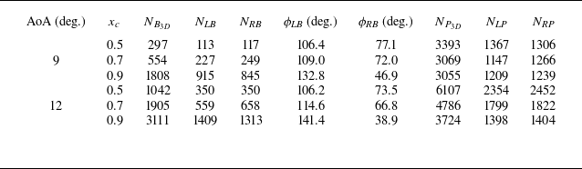
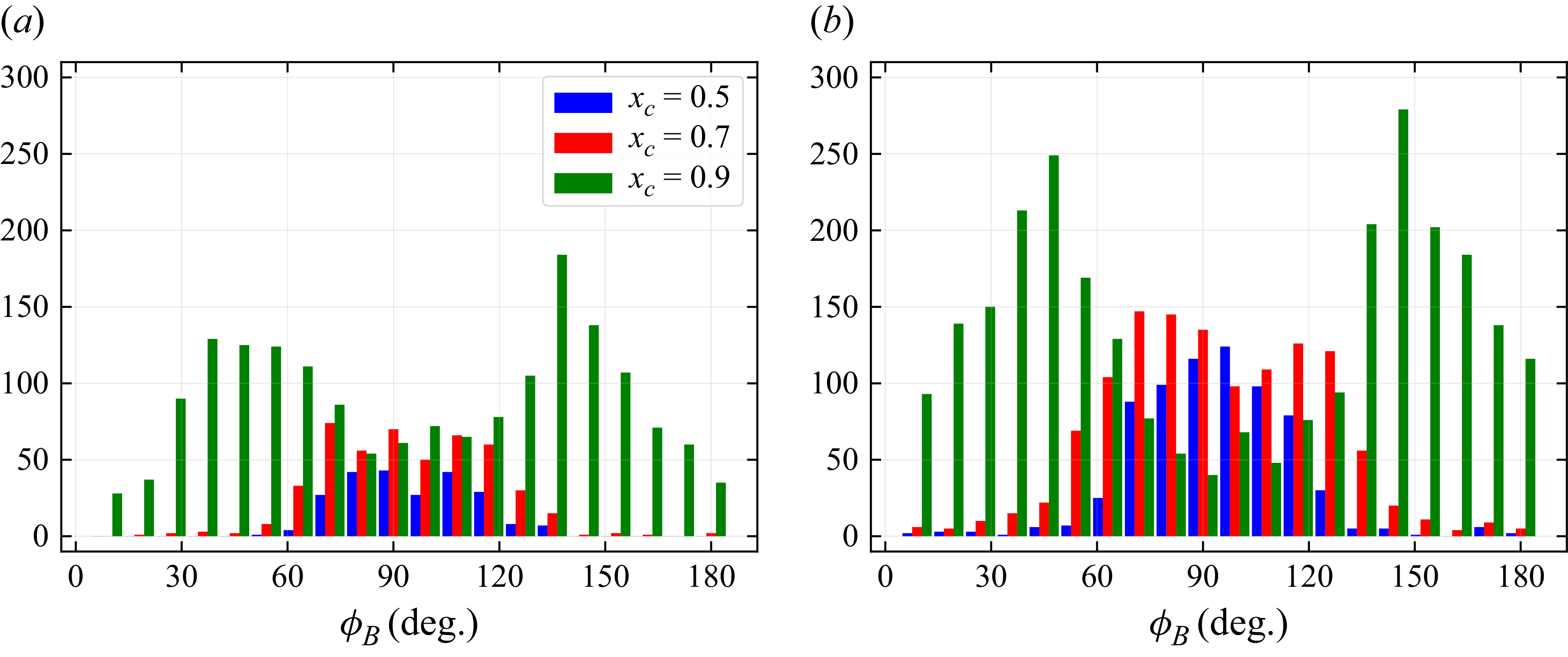
1. Introduction
Turbulent boundary layers (TBLs) play a central role in the field of fluid mechanics. Their dynamics strongly affects the performance of aerodynamic and marine devices, pipelines, ducts and turbomachinery, besides also exerting a major influence on environmental flows in the ocean and atmosphere. Despite the inherent chaotic nature of turbulence, coherent motions are commonly observed in TBLs (Robinson Reference Robinson1991), where they play a key role in the transfer of turbulent kinetic energy (TKE) between the inner and outer layers. These motions often exhibit intermittent features, commonly associated with bursting events, recognised as important contributors to TKE production in the near-wall region. Such events also impact the transition to turbulence and momentum transfer, leaving footprints on the wall shear stress, and hence, impacting drag production.
The dynamics of TBLs was investigated in an earlier study by Kline et al. (Reference Kline, Reynolds, Schraub and Runstadler1967), who conducted experiments in an open water channel with particular emphasis on the near-wall region. By combining flow visualisation and measurements, the authors analysed the coherent motions in TBLs developing under various pressure gradients. They concluded that the dynamics of the streak breakup, beginning with its formation, lift-up, oscillation, bursting and ejection, plays an important role in the entire TBL, being a dominant process in the energy transfer between the inner and outer regions. The authors also observed that, in the presence of adverse pressure gradients (APGs), bursting events exhibited greater intensity, whereas under favourable pressure gradients (FPGs), this mechanism was attenuated. Corino & Brodkey (Reference Corino and Brodkey1969) employed flow visualisation techniques to characterise fluid motions in the vicinity of a pipe wall. Their work highlighted the importance of ejections, particularly how their interaction with the mean shear contributes to the maintenance of turbulence. These previous studies drew attention to the significance of coherent motions, contributing to subsequent analyses of the mechanisms governing TKE production and the wall shear stress.
The role of coherent motions in the Reynolds shear stress was investigated by Wallace, Eckelmann & Brodkey (Reference Wallace, Eckelmann and Brodkey1972) through experiments in turbulent channel flows. The authors analysed the individual contributions of streamwise and wall-normal velocity fluctuations, concluding that ejection events had a dominant effect on the Reynolds stress and TKE distributions. In the same year, Willmarth & Lu (Reference Willmarth and Lu1972) employed conditional sampling analysis to identify intense bursting events that exhibited large contributions to Reynolds stresses and TKE. Such extreme events corresponded to ejection motions. The studies by Wallace et al. (Reference Wallace, Eckelmann and Brodkey1972) and Willmarth & Lu (Reference Willmarth and Lu1972) were the precursors of quadrant analysis, a technique that classifies streamwise and wall-normal velocity fluctuations within a Cartesian plane, where the second and fourth quadrants correspond to ejections and sweeps, respectively, and the first and third quadrants represent outward and inward interactions. Although the previous references have emphasised the role of ejections, Offen & Kline (Reference Offen and Kline1974) investigated the relationship between bursts and sweeps in a TBL using dye injection and bubble wire visualisation. Their observations revealed that the bursting phenomenon follows a cycle, beginning with a sweep originating in the logarithmic region, which generates disturbances that ultimately trigger a burst. This finding led to the model of the aforementioned bursting ‘quasi-cycle’ process (Offen & Kline Reference Offen and Kline1975).
Beyond the visualisation techniques used to understand the dynamics of sweeps and ejections in TBLs, conditional analysis from hot-wire probe measurements has also been employed (Wallace et al. Reference Wallace, Eckelmann and Brodkey1972; Willmarth & Lu Reference Willmarth and Lu1972). Morrison, Subramanian & Bradshaw (Reference Morrison, Subramanian and Bradshaw1992) applied conditional sampling techniques to isolate the contributions of sweeps and ejections in zero-pressure-gradient (ZPG) boundary layers developing over smooth and rough-to-smooth walls. A complete description of the behaviour of sweeps and ejections in both inner and outer layers revealed that both types of motion exhibited high spatial coherence, efficiently transporting momentum, supporting the hypothesis that they form part of a large-scale inertial structure.
Previous investigations have primarily focused on elucidating the dynamics of coherent motions and their role in momentum transport and TKE production. It was shown that these motions are crucial for the near-wall dynamics (Jiménez & Pinelli Reference Jiménez and Pinelli1999), directly impacting the wall shear stress. This aspect was studied by Orlandi & Jiménez (Reference Orlandi and Jiménez1994), who performed simulations of a simplified two-dimensional model of a plane transversal to the flow, combined with the minimal flow unit methodology (Jiménez & Moin Reference Jiménez and Moin1991). The numerical model consisted of a pair of counter-rotating vortices embedded in a uniform streamwise shear field. The results showed that the longitudinal velocity profile was lifted at the centre of the vortex pair, producing a low-speed streak, while the outer regions were forced toward the wall, generating regions of high wall shear. The latter mechanism was associated with a sweep motion that transported high-speed fluid from the outer layer to the near-wall region.
Understanding the physical process related to wall shear stress provides the foundation for developing flow control strategies. Moreover, such analysis offers insights into drag generation mechanisms in cases of positive stress, and reverse-flow dynamics in cases of negative stress, the latter being related to local boundary-layer separation (Simpson Reference Simpson1989). In addition, patterns of instantaneous wall shear stress reveal the footprints of near-wall streaks, whose modulations reflect the influence of large-scale outer-layer structures (Abe, Kawamura & Choi Reference Abe, Kawamura and Choi2004). Special attention should be given to the study of extreme wall shear-stress events, as they significantly contribute to skin-friction drag and local separation. Understanding their dynamics is essential for advancing turbulence modelling and developing strategies for drag reduction.
When considering the generation of extreme positive wall shear-stress events, a mechanism similar to that described by Orlandi & Jiménez (Reference Orlandi and Jiménez1994) is observed. Sheng, Malkiel & Katz (Reference Sheng, Malkiel and Katz2009) performed channel flow experiments at friction Reynolds number
 $\textit{Re}_\tau = 1470$
using digital holographic microscopy to simultaneously measure both wall shear-stress components and the three-dimensional velocity field. Their analysis showed that regions of large wall shear-stress magnitude are typically associated with single or paired quasi-streamwise vortices that induce a sweep motion and spanwise momentum transport. The authors also found that regions of low skin friction were related to paired streamwise vortices that promoted ejection motions. Subsequently, Hutchins et al. (Reference Hutchins, Monty, Ganapathisubramani, H.C.H. and Marusic2011) conducted experiments in a high-Reynolds-number TBL (
 $\textit{Re}_\tau = 14\,150$
) using hot-film shear-stress sensors together with a traversing hot-wire to conditionally sample high and low skin-friction events. They reported that high-speed structures associated with high positive skin friction have an important role in the modulation of small-scale activity near the wall, whereas this activity diminishes away from the wall. The opposite trend was observed for low-speed structures, which are associated with low skin-friction events and exhibit greater intensity in the modulation of small scales away from the wall.
The relative contributions of small- and large-scale structures (LSSs) to Reynolds shear stress were investigated by Gomit, de Kat & Ganapathisubramani (Reference Gomit, de Kat and Ganapathisubramani2018) through particle image velocimetry together with wall shear-stress sensors in a high-Reynolds-number TBL experiment with
 $\textit{Re}_\tau \approx 4000$
. In their study, the LSSs were defined as motions with characteristic lengths greater than the boundary-layer thickness
 $\delta$
, whereas small-scale structures corresponded to scales ranging from approximately 100 wall units up to
 $\delta$
. They decomposed the probability density function (PDF) histogram of the friction velocity fluctuations into four quartiles, each one containing
 $25\,\%$
of the events. The first two quartiles corresponded to the negative portion of the distribution, whereas the remaining two quartiles were associated with positive fluctuation events. Their findings revealed that extreme events associated with low and high instantaneous speeds, depicted respectively in the first and last quartiles, are predominantly associated with large and small scales, respectively, both contributing substantially to the total Reynolds shear stress.
The topic of extreme wall shear-stress events was further examined by Pan & Kwon (Reference Pan and Kwon2018), who analysed snapshots from a direct numerical simulation (DNS) dataset of a TBL developing over a smooth wall at
 $\textit{Re}_\tau = 1500$
. They assessed the role of outer-layer LSSs in both extreme positive and negative wall shear events. It was found that extreme positive events are linked to sweep motions that transport high-momentum fluid from the outer layer towards the wall, in a mechanism similar to a splatting process. More recently, Guerrero, Lambert & Chin (Reference Guerrero, Lambert and Chin2020) performed DNS of turbulent pipe flows across a range of Reynolds numbers (
 $170 \leqslant \textit{Re}_\tau \leqslant 2003$
) to investigate the mechanisms underlying extreme positive and negative wall shear-stress events. Their conditional analysis demonstrated that extreme positive events are related to strong quasi-streamwise vortices in the buffer region, which transport high streamwise momentum from the overlap and outer layers towards the wall.
Negative wall shear-stress events can also occur in wall-bounded turbulent flows, despite early claims that such events would not exist (Eckelmann Reference Eckelmann1974). Subsequent experimental and numerical investigations have demonstrated that these events, although rare, are indeed present in turbulent flows, being associated with the occurrence of backflows. Lenaers et al. (Reference Lenaers, Li, Brethouwer, Schlatter and Örlü2012) performed DNS of turbulent channel flows at
 $180 \leqslant \textit{Re}_\tau \leqslant 1000$
, to quantify the characteristics of backflow events. They observed a Reynolds-number dependence where backflow events become more frequent and occur farther away from the wall, as the friction Reynolds number increases. Their results also demonstrated that backflow regions exhibit an average diameter of 20 viscous units, and are caused by an oblique vortex located outside the viscous sublayer. Using images of flexible micropillars, Brücker (Reference Brücker2015) demonstrated the presence of backflows in a ZPG TBL over a flat plate. This previous work showed that backflow regions coincide with areas of large spanwise gradients of wall shear stress due to splatting. The presence of backflow events was also verified experimentally by Willert et al. (Reference Willert2018) in a ZPG TBL developing over a flat plate. Particle image velocimetry measurements were conducted for
 $800 \leqslant \textit{Re}_\tau \leqslant 2400$
, showing that the average reverse-flow region measured approximately 30 wall units in length and 5 wall units in height, in agreement with the findings of Lenaers et al. (Reference Lenaers, Li, Brethouwer, Schlatter and Örlü2012). More recently, Cardesa et al. (Reference Cardesa, Monty, Soria and Chong2019) analysed DNS datasets of turbulent channel flow at friction Reynolds numbers
 $550 \leqslant \textit{Re}_\tau \leqslant 2000$
, and characterised regions with negative streamwise velocity to investigate the dynamics of backflow events. They found that backflow structures result from complex interactions between regions of high and low spanwise vorticity away from the wall. It was also shown that these structures become more elongated in the spanwise direction at higher wall-normal positions.
Guerrero et al. (Reference Guerrero, Lambert and Chin2020) examined extreme negative wall shear-stress events associated with backflows and reported that their formation can be associated either with a single strong oblique vortex, or with a pair of counter-rotating vortices that transport momentum from the wall toward the outer layer. In a follow-up study of pipe flows, Guerrero, Lambert & Chin (Reference Guerrero, Lambert and Chin2022) observed that backflow events are often preceded by the asymmetric collision of two LSSs of high and low speed, with streamwise length of approximately three times the pipe radius. The result of this interaction is a vortex that generates the negative wall shear stress and triggers the breakdown of the low-speed LSS. In such cases, high momentum from the high-speed structure is transported from the outer region towards the wall, intercepting the low-speed structure located near the wall, engulfing a small portion of the latter. The authors associated this phenomenon with the near-wall self sustaining process of TBLs.
The influence of APGs on backflow events was examined by Vinuesa, Örlü & Schlatter (Reference Vinuesa, Örlü and Schlatter2017) through analysis of a DNS dataset of a NACA4412 airfoil. The authors focused on the TBL developing on the suction side, which exhibits an increasing APG in the streamwise direction and a maximum friction Reynolds number of
 $\textit{Re}_\tau = 373$
. They reported backflow levels of
 $30\,\%$
near the trailing edge, where a very strong APG condition is reached. Conditional analysis based on extreme wall shear-stress events indicated that, under strong APG conditions, the wall shear-stress orientation has a higher probability of aligning either with or against the free-stream direction. More recently, Bross, Fuchs & Kähler (Reference Bross, Fuchs and Kähler2019) investigated the interaction of coherent flow structures in an APG TBL at
 $\textit{Re}_\tau = 2500$
using particle tracking velocimetry. Their findings indicate that backflow events are triggered when a low-momentum LSS interacts with and decelerates an existing low-speed streak. The mechanism described by the authors differs from those reported by Guerrero et al. (Reference Guerrero, Lambert and Chin2020) and Guerrero et al. (Reference Guerrero, Lambert and Chin2022), highlighting the uncertainty regarding the influence of APGs on the generation of both positive and negative extreme wall shear-stress events.
When considering APG TBLs, several studies have examined how APGs affect the turbulence statistics, for instance, the energisation of outer-layer structures and the amplification of large-scale motions (Monty, Harun & Marusic Reference Monty, Harun and Marusic2011; Harun et al. Reference Harun, Monty, Mathis and Marusic2013). Although the fundamental energy transfer mechanisms remain broadly similar to those in ZPG flows (Gungor, Maciel & Gungor Reference Gungor, Maciel and Gungor2022; Deshpande & Vinuesa Reference Deshpande and Vinuesa2024), their intensity is substantially modified by the presence of an APG. Recent work has also demonstrated that a FPG upstream of an APG can strongly influence the inner-layer dynamics, while exerting a weaker effect on the outer region (Parthasarathy & Saxton-Fox Reference Parthasarathy and Saxton-Fox2023). Moreover, studies of airfoils at high angles of attack (AoA) revealed that the resulting strong APGs affect not only the Reynolds stresses but also the TKE production mechanisms and the anisotropy along the TBL (Silva & Wolf Reference Silva and Wolf2024). While these studies focused on fundamental turbulence statistics of APG TBLs, they did not address the occurrence of extreme events or their associated coherent motions.
To advance the understanding of how APGs influence the near-wall coherent structures responsible for momentum transport and wall shear-stress generation, the present work examines the effect of increasing APGs on the turbulent structures responsible for extreme positive and backflow events. Particular attention is given to the spatial support and dynamics of sweep and ejection motions, and their interactions with near-wall streaks and vortical structures. To this end, wall-resolved large eddy simulations (LES) are performed for a NACA0012 airfoil at AoA of
 $9$
and
 $12^{\circ}$
, focusing on the development of the TBL along the suction side. The simulations are conducted at a chord-based Reynolds number of
 $\textit{Re} = 4 \times 10^5$
and a free-stream Mach number of
 $M = 0.2$
. Despite the relatively high AoA, no mean flow separation is observed. Further details of the flow configurations analysed, as well as the theoretical formulation and numerical methods employed, are presented in § 2. The characterisation of the mean flow, including the Rotta–Clauser pressure-gradient parameter, a study of momentum balances and the decomposition of the Reynolds shear stress, is discussed in § 3. Section 4 investigates the occurrence of extreme wall shear-stress events under mild and strong APGs. This analysis is supported by a statistical characterisation of events using PDFs and space–time correlations (§ 4.1); conditional statistics of extreme events, focusing on the evolution of mean flow profiles and the contribution of individual Reynolds shear-stress quadrants (§ 4.2); and the examination of the coherent structures responsible for backflow and extreme positive event dynamics (§ 4.3). Finally, the main conclusions regarding the role of APGs in extreme shear-stress events and their associated coherent structures are summarised in § 5.
2. Theoretical and numerical methodology
Wall-resolved LES are conducted to solve the compressible mass, momentum and energy balance equations written in general curvilinear coordinates
 $(\xi ^i \mbox{, } i=1,2,3)$
, in which the velocity vector is represented in the contravariant
 $(U^i)$
form. The balance equations are expressed as
 \begin{equation} \frac {\partial \rho }{\partial t} + \big(\rho U^j\big)_{,j} = 0, \end{equation}
 \begin{equation} \frac {\partial \rho U^i}{\partial t} +\big (\rho U^iU^j\big )_{,j} = - \big (g^{ij}p\big )_{,j} + \tau ^{ij}_{,j} \end{equation}
and
 \begin{equation} \frac {\partial E}{\partial t} +\big [(E+p)U^j \big ]_{,j} = -q^j_{j} + \big (\tau ^{ij}g_{ik}U^k\big )_{,j}, \end{equation}
where time, density and pressure are denoted by
 $t, \rho $
and
 $p$
, respectively. The contravariant and covariant metric tensors are represented by
 $g^{ij}$
and
 $g_{ij}$
, respectively, and subscripts preceded by comma
 $(.)_{,j}$
indicate covariant derivatives (see Appendix A and Aris Reference Aris1989 for more details). The Einstein summation convention applies for repeated indices.
The equations are solved in a non-dimensional form using the free-stream properties and the airfoil chord
 $L$
. Further details regarding the non-dimensionalisation procedure are provided by Lui et al. (Reference Lui, Ricciardi, Wolf, Braun, Rahbari and Paniagua2022). Additionally, considering a Newtonian fluid that obeys Fourier’s law, the viscous stress tensor
 $\tau ^{ij}$
, heat flux
 $q^j$
and total energy
 $E$
are described, respectively, by
 \begin{equation} \tau ^{ij} = \mu \dfrac {M}{\textit{Re}}\left (g^{jk}U^i_{,k} + g^{ik}U^j_{,k} -\dfrac {2}{3}g^{ij}U^k_{,k}\right )\!, \end{equation}
 \begin{equation} q^j = -\dfrac {M}{\textit{RePr}}\mu g^{ij}T_{,i} \end{equation}
and
 \begin{equation} E = \dfrac {p}{\gamma -1}+\dfrac {1}{2}\rho g_{ij}U^iU^j . \end{equation}
Here,
 $\textit{Re}$
is the Reynolds number based on the airfoil chord and free-stream velocity,
 $M$
is the free-stream Mach number,
 $\textit{Pr}$
is the Prandtl number and
 $T$
is the temperature. Assuming a calorically perfect gas, the system of equations is closed by the equation of state
 \begin{equation} p = \dfrac {(\gamma -1)}{\gamma }\rho T, \end{equation}
where
 $\gamma$
is the ratio of specific heats. The dynamic viscosity
 $\mu$
is computed by Sutherland’s law, expressed by
 \begin{equation} \mu = \left [(\gamma -1)T\right ]^{\frac {3}{2}}\dfrac {1+S_\mu }{T(\gamma -1)+S_\mu }, \end{equation}
where
 $S_\mu$
is the non-dimensional Sutherland constant.
The computational domain is constructed using an overset grid approach, in which an O-type grid, conforming to the airfoil surface, is embedded within a background Cartesian H-type grid. The present O-grid is built using a hyperbolic grid generator that enforces orthogonality near the airfoil surface. A fine grid point distribution along the suction side maintains orthogonal grid lines throughout the TBL, as confirmed by the near-zero metric tensor component
 $g_{12}$
(more details provided as supplementary material). Hence, along the entire suction side, grid lines
 $\xi ^1$
and
 $\xi ^2$
are tangent and normal to the airfoil surface, respectively. In order to facilitate notation, properties evaluated in these directions are written with subscripts
 $t$
and
 $n$
. Throughout this work, the instantaneous velocity components in contravariant form are denoted by
 $U^1 = U_t$
,
 $U^2 = U_n$
and
 $U^3 = W$
, representing the wall-tangential, wall-normal and spanwise components, respectively, with respect to the curvilinear coordinates
 $\xi ^1$
,
 $\xi ^2$
and
 $\xi ^3$
. When needed, instantaneous velocities in the Cartesian coordinate system are written as
 $U, V$
and
 $W$
with respect to the
 $x$
,
 $y$
and
 $z$
directions, respectively. It is important to highlight that, for the present simulations with spanwise homogeneous flows,
 $\xi ^3 = z$
.
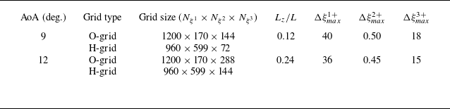
Grid details and near-wall resolution in wall units for
 $9$
and
 $12^{\circ}$
AoA.

The spatial derivatives of the governing equations are discretised using a sixth-order compact finite-difference scheme implemented on a staggered grid (Nagarajan, Lele & Ferziger Reference Nagarajan, Lele and Ferziger2003). The communication between the overlapping zones of the O- and H-grids is ensured using a fourth-order compact interpolation scheme (Bhaskaran & Lele Reference Bhaskaran and Lele2010). To suppress numerical instabilities caused by grid stretching and interpolation across grid interfaces, a sixth-order compact filter (Lele Reference Lele1992) is applied away from the airfoil wall, as shown by Silva & Wolf (Reference Silva and Wolf2024). The temporal integration of the governing equations is performed using a hybrid implicit–explicit approach. An implicit second-order scheme is employed on the O-grid, whereas an explicit third-order Runge–Kutta scheme is applied on the Cartesian mesh. Characteristic boundary conditions based on Riemann invariants are applied in the far field, together with a sponge layer that prevents reflections of acoustic waves. At the airfoil surface, no-slip adiabatic conditions are imposed and in the spanwise direction periodic boundary conditions are applied. The present numerical framework has been validated in previous studies of compressible flows over airfoils for different conditions (Wolf et al. Reference Wolf, Azevedo and Lele2012a , Reference Wolf, Lele, Jothiprasad and Cheungb ; Ricciardi & Wolf Reference Ricciardi and Wolf2022; Lui et al. Reference Lui, Ricciardi, Wolf, Braun, Rahbari and Paniagua2022; Miotto et al. Reference Miotto, Wolf, Gaitonde and Visbal2022). Further details about the numerical methodology can be found in Nagarajan et al. (Reference Nagarajan, Lele and Ferziger2003), Bhaskaran & Lele (Reference Bhaskaran and Lele2010) and Wolf (Reference Wolf2011).
The simulations are performed for a NACA0012 airfoil at
 $9$
and
 $12^{\circ}$
angle of attack, with free-stream Mach number
 $M = 0.2$
and chord-based Reynolds number
 $\textit{Re} = 4 \times 10^5$
. The airfoil trailing edge is rounded at
 $99\,\%$
of the chord with a curvature radius of
 $0.0015L$
to obtain smooth metric tensors. Table 1 presents the number of grid points
 $ (N_{\xi ^1} \times N_{\xi ^2} \times N_{\xi ^3} )$
for the individual grids, as well as the respective spatial resolution in terms of wall units for both simulations. The present simulations meet the requirements for wall-resolved LES as recommended by Georgiadis, Rizzetta & Fureby (Reference Georgiadis, Rizzetta and Fureby2010). The airfoil spanwise length
 $L_z$
is also presented in table 1. The present values of this parameter are chosen to resolve at least 5 times the length of the boundary-layer displacement thickness at the trailing edge in order to minimise the effects of spanwise periodic boundary conditions. As shown by Silva & Wolf (Reference Silva and Wolf2024), the spanwise two-point correlations of velocity fluctuations decay significantly along the span for various positions along the entire airfoil chord.
A numerical tripping is applied on the suction side of the airfoils in the region
 $0.04 \leqslant x_c \leqslant 0.09$
to promote bypass transition and prevent the formation of Tollmien–Schlichting waves, where
 $x_c$
is the position measured along the airfoil chord, as shown in figure 1. The tripping consists of a random spanwise and streamwise disturbance, introduced with minimal amplitude to trigger transition without introducing excessive perturbations to the flow. As a consequence of tripping and the APG, a TBL develops along the suction side of the airfoils, whereas the pressure side maintains a laminar boundary layer. Figures 1(a) and 1(c) present snapshots for the
 $9$
and
 $12^{\circ}$
angle of attack simulations, respectively, illustrating the presence of fine-scale turbulent structures. Figures 1(b) and 1(d) present the mean flow fields, where the insets provide an enlarged view of the trailing-edge region demonstrating that, despite the high angle of attack, the mean flow remains attached upstream of the trailing edge. More details about the flow conditions, tripping set-up and grid resolution can be found in Silva & Wolf (Reference Silva and Wolf2024).
Simulation results presented for
 $9$
and
 $12^{\circ}$
angle of attack in the top and bottom rows, respectively. Iso-surfaces of
 $Q$
-criterion coloured by the
 $U$
velocity component normalised by the free-stream velocity
 $U_\infty$
are presented in (a) and (c). Mean flow fields (
 $U/U_\infty$
) are depicted in (b) and (d) using the same contour levels of the left column plots.

3. Mean flow characterisation
This section presents the mean flow characterisation of the investigated TBLs. The results are expressed using a Reynolds decomposition, where the velocity components are written as
 $U^i = \langle U^i\rangle + u^i$
. Here, the angle brackets denote the combined temporal and spanwise average, while the lowercase letters represent the corresponding fluctuations. Similarly, scalar variables are expressed as
 $f = \langle f\rangle + f'$
, with the primed quantities denoting fluctuations.
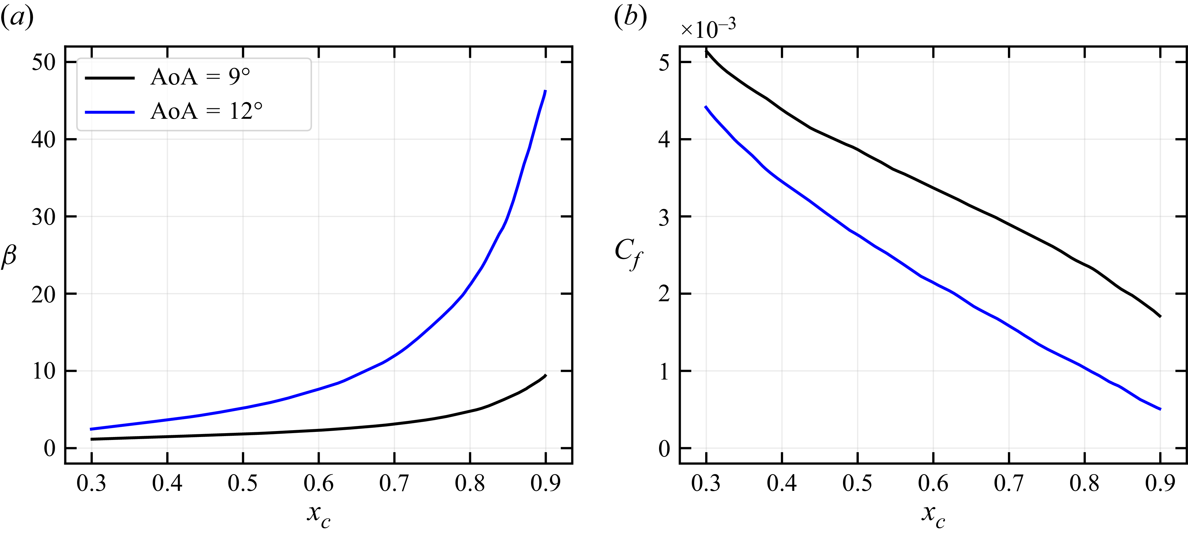
Evolution of the (a) Rotta–Clauser pressure-gradient parameter
 $\beta$
and (b) skin-friction coefficient
 $C_f$
along the airfoil chord.

Due to the high AoA, the TBLs develop over increasing APGs that can be locally quantified by the Rotta–Clauser pressure-gradient parameter
 $\beta = (\delta ^*/\langle \tau _w\rangle )\mathrm{d}\langle p\rangle /\mathrm{d}x_t$
. Here,
 $\delta ^*$
is the displacement thickness,
 $\tau _w = \mu (\langle U^1\rangle )_{,2}$
is the wall shear stress and
 $\mathrm{d}\langle p\rangle /\mathrm{d}x_t= (\langle p\rangle )_{,1}$
is the wall pressure gradient in the direction tangential to the airfoil surface. Figure 2 presents the chordwise distribution of
 $\beta$
and the friction coefficient
 $C_f = 2\langle \tau _w\rangle /\rho _\infty U_\infty ^2$
for the
 $9$
and
 $12^{\circ}$
AoA. In these figures, we present the results starting from the position
 $x_c = 0.30$
to avoid the influence of the tripping region. Figure 2(a) shows that differences in angle of attack produce significant changes in the pressure gradient, particularly near the trailing edge, where the
 $12^{\circ}$
case exhibits a pronounced increase. Moreover, the angle of attack directly influences the rate of change of the pressure gradient, thereby affecting the boundary-layer evolution through flow-history effects. In figure 2(b) the chordwise evolution of the friction coefficient
 $C_f$
reflects the APG effect, where an increasing APG is associated with a reduction in
 $C_f$
. In order to further investigate the effects of mild, moderate and strong APG conditions, the subsequent analyses will place particular emphasis on the airfoil chord positions
 $x_c = 0.5, 0.7$
and
 $0.9$
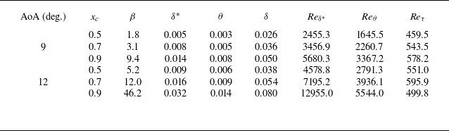
. The integral properties of these specific positions are presented in table 2 for both simulations. As one would expect, all quantities present an increase towards the most downstream location analysed, except for the friction Reynolds number (
 $\textit{Re}_\tau$
). This trend arises because the friction velocity reduces under the increasing APG more rapidly than the boundary-layer thickness grows, as shown by Silva & Wolf (Reference Silva and Wolf2024).
Properties of the TBLs at selected chordwise positions, including the pressure-gradient parameter
 $\beta$
; the displacement, momentum and boundary-layer thicknesses (
 $\delta ^*$
,
 $\theta$
and
 $\delta$
); the Reynolds numbers based on displacement and momentum thicknesses (
 $\textit{Re}_{\delta ^*}$
and
 $\textit{Re}_\theta$
); and the friction Reynolds number
 $\textit{Re}_\tau$
. Boundary-layer integral parameters are normalised by the chord length.

An analysis of the mean momentum balance equations is conducted to elucidate the influence of the APG on the individual terms comprising the balance. As discussed in § 2, the Navier–Stokes equations are solved in general curvilinear coordinates using contravariant vector components, which require the use of covariant derivatives. This approach enables a direct evaluation of the flow properties along the tangential and wall-normal directions. Within this framework, the mean momentum equations can be expressed in the tangential and wall-normal directions, respectively, as
 \begin{equation} \big \langle U^j\big \rangle \big (\big \langle U^1\big \rangle \big )_{,j} + \frac {1}{\left \langle \rho \right \rangle } \big(g^{1j}\left \langle p\right \rangle \big)_{,j} + \big \langle u^1 u^j\big \rangle _{,j} - \frac {1}{\left \langle \rho \right \rangle }\big \langle \tau ^{1j} \big \rangle _{,j} = 0, \end{equation}
and
 \begin{equation} \big \langle U^j\big \rangle \big (\big \langle U^2\big \rangle \big )_{,j} + \frac {1}{\left \langle \rho \right \rangle } \big(g^{2j}\left \langle p\right \rangle \big)_{,j} + \big \langle u^2 u^j\big \rangle _{,j} - \frac {1}{\left \langle \rho \right \rangle }\big \langle \tau ^{2j} \big \rangle _{,j} = 0. \end{equation}
Prior to computing the balances, all terms in the equations are expressed in physical components. This procedure involves the use of metric tensors to compute unitary covariant basis vectors (Aris Reference Aris1989), as shown in Appendix A. The individual terms of the mean tangential momentum equation (3.1) and mean wall-normal momentum equation (3.2) are presented in figures 3 and 4, respectively. In these figures, solid lines denote the total contribution obtained by summation over the repeated index
 $j$
, while the dashed and dot-dashed lines represent the individual contributions from the
 $j = 1$
and
 $j = 2$
components, respectively. The top row shows the results for the
 $9^{\circ}$
simulation, while the bottom row depicts those for the
 $12^{\circ}$
case. The analysis is performed for chordwise positions
 $x_c = 0.5$
,
 $0.7$
and
 $0.9$
. All terms are expressed in non-dimensional form using the inner scaling
 $u_\tau ^3/\nu$
, where
 $u_\tau$
is the friction velocity and
 $\nu$
is the kinematic viscosity. For the
 $9^{\circ}$
case, a constant y-axis scale is used across different chordwise positions to facilitate direct comparison of the balance terms as the APG increases. For the
 $12^{\circ}$
case, the y-axis scale is modified at
 $x_c = 0.9$
to improve visualisation, since most terms appearing in the balance have considerably higher values due to the inner scaling (Maciel et al. Reference Maciel, Wei, Gungor and Simens2018).
Analysis of figure 3 indicates that the pressure-gradient component
 $\langle \rho \rangle ^{-1}(g^{1j}\langle p\rangle )_{,j}$
remains nearly constant in the wall-normal direction across both simulations and at all chordwise locations, consistent with boundary-layer theory. This pressure gradient is solely dominated by the wall-tangential contribution
 $\langle \rho \rangle ^{-1}(g^{11}\langle p\rangle )_{,1}$
, which reflects the pressure variation along the airfoil surface. At the wall, a balance is established between pressure and viscous forces. Within the buffer layer, the viscous term
 $\langle \tau ^{1j} \rangle _{,j}$
, together with the pressure gradient, is counteracted by the gradient of the Reynolds stresses
 $\langle u^1 u^j\rangle _{,j}$
. As expected, both the viscous and Reynolds stresses are primarily constituted by their wall-normal components
 $\langle \tau ^{12} \rangle _{,2}$
and
 $\langle u^1 u^2\rangle _{,2}$
, respectively. In the buffer layer and logarithmic region, particularly at downstream positions where the APG intensifies, the mean tangential convection term
 $\langle U^j\rangle (\langle U^1\rangle )_{,j}$
becomes increasingly significant in the momentum balance. Its contribution, however, is more pronounced in the outer layer, where it is primarily counterbalanced by the pressure gradient and, to a lesser extent, by the Reynolds-stress term.
Individual terms of the wall-tangential mean momentum equation at chordwise positions
 $x_c = (\textit {a,d})\,0.5$
, (b,e)
 $0.7$
and (c,f)
 $0.9$
. Solid lines denote the total contribution obtained by summation over the repeated index
 $j$
in (3.1), whereas dashed and dot-dashed lines represent the individual contributions from the
 $j=1$
and
 $j=2$
components, respectively. Top and bottom rows show results for AoA
 $9$
and
 $12^{\circ}$
, respectively. All terms are non-dimensionalised by
 $u_\tau ^3/\nu$
.

The terms involving the divergence of the Reynolds-stress tensor characterise the exchange of momentum between the fluctuating and mean velocity flow fields (Kitsios et al. Reference Kitsios, Sekimoto, Atkinson, Sillero, Borrell, Gungor, Jiménez and Soria2017). Positive values correspond to momentum transfer from the fluctuations to the mean flow, whereas negative values indicate the opposite. The predominance of the
 $ \langle u^1 u^2\rangle _{,2}$
component highlights the central role of the Reynolds shear stress in the momentum transfer across layers. In the inner layer, the negative peak reflects intense transfer from the mean field to the fluctuations, while in the outer layer a positive peak emerges, indicating the reversed trend. The wall-normal contribution of the mean tangential convection
 $\langle U^2\rangle (\langle U^1\rangle )_{,2}$
becomes increasingly relevant in the outer layer as the APG intensifies. Nevertheless, the tangential component
 $\langle U^1\rangle (\langle U^1\rangle )_{,1}$
, which exhibits a more pronounced peak, remains the dominant contribution. This behaviour reflects the fact that boundary-layer deceleration is primarily driven by the APG, thereby shaping the overall structure of the mean tangential convection. At
 $x_c = 0.9$
in the
 $12^{\circ}$
case, a strong APG develops, as shown in figure 3(f). At this location, the pressure-gradient term overcomes the peak of the viscous term in the buffer layer, differently from the other chordwise positions. Moreover, in the outer layer, the mean tangential convection plays a more prominent role due to both the wall-normal velocity as well as the flow deceleration, which are significantly increased in magnitude compared with all previous cases.
Individual terms of the wall-normal mean momentum equation at chordwise positions (a,d)
 $x_c = 0.5$
, (b,e)
 $0.7$
and (c,f)
 $0.9$
. Solid lines denote the total contribution obtained by summation over the repeated index
 $j$
in (3.2), whereas dashed and dot-dashed lines represent the individual contributions from the
 $j=1$
and
 $j=2$
components, respectively. Top and bottom rows show results for AoA
 $9$
and
 $12^{\circ}$
, respectively. All terms are non-dimensionalised by
 $u_\tau ^3/\nu$
.

Figure 4 exhibits the individual terms of the mean momentum equation in the wall-normal direction, expressed as (3.2). It is observed that the Reynolds-stress
 $\langle u^2 u^j\rangle _{,j}$
and pressure-gradient
 $\langle \rho \rangle ^{-1}(g^{2j}\langle p\rangle )_{,j}$
terms dominate the balance, particularly within the inner layer. In this region, these terms display positive and negative peaks, respectively, with the wall-normal components (
 $j=2$
) providing the largest contribution. In the outer layer, a small negative peak is observed for the Reynolds stress, while a positive peak arises for the pressure-gradient component. The presence of the wall-normal convective term
 $\langle U^j\rangle (\langle U^2\rangle )_{,j}$
is also noticed in the outer layer. For mild APGs, this latter term is negative due to the tangential component
 $\langle U^1\rangle (\langle U^2\rangle )_{,1}$
, whereas for the strong APG case shown in figure 4(f), it becomes positive due to the contributions of both tangential and wall-normal components. A wall-normal convection effect has been observed for TBLs under strong APGs (Vinuesa et al. Reference Vinuesa, Negi, Atzori, Hanifi, Henningson and Schlatter2018). Here, we show that two mechanisms compete: the mean flow convection exchanges energy with
 $\langle u^2 u^2\rangle _{,2}$
and, near the edge of the boundary layer, a mild wall-normal FPG provides an outward acceleration of the mean flow.
The present findings are consistent with those reported by Kitsios et al. (Reference Kitsios, Sekimoto, Atkinson, Sillero, Borrell, Gungor, Jiménez and Soria2017), who conducted DNS of TBLs developing over a flat plate with far-field boundary conditions set to develop different pressure gradients. These authors examined boundary layers with ZPG as well as with mild (
 $\beta = 1$
) and strong
 $(\beta = 39)$
APGs, the latter closely resembling the conditions investigated in the current work for
 $12^{\circ}$
, near the trailing edge. However, unlike their case, the present study considers non-equilibrium boundary layers arising from streamwise-varying pressure gradients and upstream flow-history effects. Kitsios et al. (Reference Kitsios, Sekimoto, Atkinson, Sillero, Borrell, Gungor, Jiménez and Soria2017) showed that the APG increases the convective terms due the rise in mean velocity gradients, thereby enhancing the production of turbulent fluctuations. They also reported a net transfer of streamwise momentum from the mean flow to the fluctuating field in the inner layer, with the opposite trend in the outer layer, reflected by the divergence of the Reynolds stresses. To clarify the mechanisms governing this momentum transfer, we perform a quadrant analysis to isolate the contributions of ejections (
 $Q2$
), sweeps (
 $Q4$
), and outward and inward interactions (
 $Q1$
and
 $Q3$
, respectively).
Decomposition of the wall-normal derivative of the Reynolds shear stress into quadrant contributions at chordwise positions (a,d)
 $x_c = 0.5$
, (b,e)
 $0.7$
and (c,f)
 $0.9$
. The top and bottom rows present results for
 $9$
and
 $12^{\circ}$
AoA, respectively. All quantities are non-dimensionalised by
 $u_\tau ^3/\nu$
.

As shown in figure 3, the dominant contributor to the divergence of the Reynolds-stress tensor in the tangential momentum balance is the shear term
 $\langle u^1 u^2\rangle _{,2}$
. Figure 5 presents a quadrant decomposition of this term, detailing the individual contributions to momentum transfer. All quantities are non-dimensionalised using the inner scaling
 $u_\tau ^3/\nu$
. The analysis is performed at the same chordwise positions considered previously: the upper panels correspond to an angle of attack of
 $9^{\circ}$
, and the lower panels to
 $12^{\circ}$
. Sweeps and ejections emerge as the primary mechanisms for transferring momentum from the mean flow to the fluctuating field, dominating the total shear-stress term. In contrast, inward and outward interactions contribute to momentum transfer in the opposite sense. Sweeps dominate in the viscous sublayer, while ejections prevail in the buffer layer, except for the higher-pressure-gradient case, where sweeps and ejections exhibit comparable influence within the buffer region. The prominence of sweeps and ejections increases with the APG, with sweep intensities near the wall rising more rapidly than those of ejections. In the outer layer, momentum transfer reverses direction, occurring from the fluctuating to the mean field, as indicated by the positive peak in the total shear-stress term. This process results from the combined action of sweeps and ejections. Outward and inward interactions contribute similarly along the boundary layer under weaker APGs. However, outward interactions become more dominant as the APG strengthens. Although such events contribute less than sweeps and ejections overall, their influence in the viscous sublayer and buffer region increases with stronger APG.
4. Extreme wall shear-stress events under adverse pressure gradients
In this section, we characterise the occurrence of negative and positive extreme wall shear-stress events, and examine their connection with coherent motions within the TBL. As noted by Farazmand & Sapsis (Reference Farazmand and Sapsis2017), extreme events leave detectable signatures that can be identified by statistical methods. We therefore begin with a statistical analysis based on PDFs to characterise the occurrence of extreme wall shear-stress events as a function of the APGs. Next, we compute space–time correlations to examine their spatio-temporal support, followed by conditional statistics to assess the impact of extreme positive and backflow events on the mean velocity and Reynolds shear-stress profiles. Finally, we investigate the spatial and temporal evolution of the turbulent structures responsible for generating extreme wall shear stress.
4.1. Characterisation of extreme wall shear-stress events
Figures 6(a) and 6(b) present PDFs of the inner-scaled wall shear stress,
 $\tau _w^+$
, at chordwise positions
 $x_c = 0.5$
,
 $0.7$
and
 $0.9$
for AoA
 $9$
and
 $12^{\circ}$
, respectively. It can be observed from these figures that the PDFs are more skewed toward positive values of
 $\tau _w^+$
, in agreement with previous findings (Lenaers et al. Reference Lenaers, Li, Brethouwer, Schlatter and Örlü2012; Guerrero et al. Reference Guerrero, Lambert and Chin2020). This positive skewness is more pronounced at upstream locations, where the APG is weaker. In contrast, the emergence of a negative tail reflects intermittent backflow events, whose occurrence increases with the strength of the APG (Vinuesa et al. Reference Vinuesa, Örlü and Schlatter2017). Under the strongest APG condition investigated, at
 $x_c = 0.9$
and
 $12^{\circ}$
, the PDF becomes more symmetric about the mean, as seen in figure 6(b).
Probability density functions of the inner-scaled wall shear stress
 $\tau _w^+$
computed at chordwise positions
 $x=0.5$
,
 $0.7$
and
 $0.9$
for (a)
 $9$
and (b)
 $12^{\circ}$
AoA, and (c) results of the wall shear-stress fluctuations normalised by their r.m.s. value
 $\tau '_w/\tau _{w_\textit{rms}}$
. The vertical black dashed lines in (c) mark
 $\tau _w'/\tau _{w_{\textit{rms}}} = \pm 2$
, which will serve as a threshold for identifying extreme positive and backflow events.

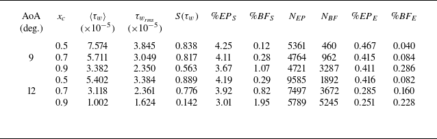
To further characterise the wall shear stress under varying APGs, table 3 reports the mean and root-mean-square (r.m.s.) values,
 $\langle \tau _w \rangle$
and
 $\tau _{w_{\textit{rms}}}$
, respectively, at different chordwise positions. The skewness values,
 $S(\tau _w)$
, are also included and corroborate the trends observed in figure 6. Specifically, skewness decreases with increasing APG, confirming that the PDFs become progressively more symmetric. As also shown in the table, the mean wall shear stress diminishes with stronger APGs, consistent with an increased likelihood of local instantaneous flow separation. Similarly, the r.m.s. values also decrease. The PDFs of the wall shear-stress fluctuations normalised by their respective r.m.s. values are presented in figure 6(c). These distributions reveal that larger negative fluctuations become more probable at chordwise positions subjected to stronger APGs, whereas positive fluctuations remain comparable up to
 $\tau _w'/\tau _{w_{\textit{rms}}} \approx 5$
. Beyond this value, stronger APGs promote larger positive deviations.
The characterisation of extreme wall shear-stress events requires the definition of a threshold. Different choices of this parameter have been adopted in previous studies. Guerrero et al. (Reference Guerrero, Lambert and Chin2020) classified any backflow event as extreme, since this criterion was appropriate for their pipe flow configuration that does not exhibit streamwise pressure-gradient variations. Vinuesa et al. (Reference Vinuesa, Örlü and Schlatter2017) investigated a TBL developing over an airfoil with a spatially varying pressure gradient. These authors used a threshold of
 $\pm 1 \tau _{w_{\textit{rms}}}$
to identify extreme wall shear-stress events. However, their negative bound did not necessarily isolate only negative wall shear-stress events.
Statistics of wall shear stress for different AoA and chordwise locations, with corresponding counts and percentages of extreme events. The mean, r.m.s. and skewness of
 $\tau _w$
are represented by
 $\langle \tau _w \rangle$
,
 $ \tau _{w_\textit{rms}}$
, and
 $S(\tau _w)$
, respectively. The percentage of samples above or below the threshold
 $\tau _w' = \pm 2 \tau _{w_{\textit{rms}}}$
is given by
 $\% \textit{EP}_{{S}}$
and
 $\% \textit{BF}_{{S}}$
. The parameters
 $N_{\textit{EP}}$
and
 $N_{\textit{BF}}$
represent the number of EP and BF realisations tracked in the temporal signals, as indicated by blue and red dots marked in figure 7. The percentages of EP and BF events are finally indicated by
 $\% \textit{EP}_{{E}}$
and
 $\% \textit{BF}_{{E}}$
, respectively.

To characterise the extreme positive (EP) and backflow (BF) events in the present flows, we first analyse the PDFs of
 $\tau _w$
, together with the temporal signals obtained at each spanwise grid point for chordwise positions
 $x_c = 0.5$
,
 $0.7$
and
 $0.9$
in both simulations. Based on these analyses, a threshold of
 $\pm 2 \tau _{w_{\textit{rms}}}$
was selected to define extreme events, which are represented by the dashed lines in figure 6(c). The selected threshold guarantees a consistent and physically meaningful definition of EP and negative (BF) events across all flow conditions considered. It corresponds to approximately 95 % separation in a normal distribution and depends only on the statistical properties of the signal. In addition, it ensures that the lower threshold always corresponds to negative wall shear-stress values, even at the chordwise location with the weakest APG, namely
 $x_c = 0.5$
of the
 $9^{\circ}$
angle of attack case, where the pressure-gradient parameter is
 $\beta = 1.8$
. As can be seen in table 3, the percentage of BF samples (
 $\textit{BF}_{{S}}$
) is lower than
 $2\,\%$
. For EP samples (
 $\textit{EP}_{{S}}$
), the criterion leads to fewer than
 $5\,\%$
of the total samples, i.e. the number of events exceeding the specified threshold.
To illustrate the temporal variation of the wall shear stress under the weakest and strongest APGs analysed, figures 7(a) and 7(b) show the time signals of
 $\tau _w^+$
at
 $x_c = 0.5$
for the
 $9^{\circ}$
angle of attack case and at
 $x_c = 0.9$
for the
 $12^{\circ}$
case, respectively. The results are presented for a single point along the span, with time normalised using convective scales. In these figures, blue and red dots mark EP and BF events. It should be noted that each dot in the figure corresponds to a single extreme event (
 $\textit{EP}_{{E}}$
or
 $\textit{BF}_{{E}}$
) in the statistics reported in table 3. The associated coloured lines delimit the temporal windows selected for each event, which span a dimensionless convective time interval
 $\Delta t_W = 0.202$
. This time window is selected to be centred on the event, not only when it exceeds the specified threshold, and is also large enough to capture its entire evolution. Specifically, the event lifespan is defined as the time interval during which the wall shear-stress signal departs from its local baseline level, reaches its extreme value and returns to the baseline level. Inspection of the signals showed that
 $\Delta t_W = 0.202$
consistently captures this complete evolution at all chordwise positions and for both AoA. Shorter windows truncate either the growth or decay phases of several events, while longer windows do not reveal additional event-related dynamics, and instead include uncorrelated fluctuations.
Examples of inner-scaled wall shear-stress signals over the full simulation duration, where (a) represents a probe at
 $x_c = 0.5$
for
 $9^{\circ}$
angle of attack and (b) represents a probe at
 $x_c = 0.9$
for
 $12^{\circ}$
angle of attack. Blue and red dots mark EP and extreme negative (BF) events, respectively, while the corresponding coloured lines represent the temporal windows of length
 $\Delta t_W = 0.202$
used to track their evolution.

After identifying the extreme events along the spanwise direction at each chordwise position, we quantify both their absolute number of occurrences and relative percentage with respect to the total number of samples collected during the simulation. The results are summarised in table 3 for both simulations at the chordwise positions under consideration. The percentage of BF samples increases with the APG, whereas the opposite trend is observed for EP samples. The highest percentage of BF samples occurs at
 $x_c = 0.9$
in the
 $12^{\circ}$
case. A similar trend is found for the number of BF events (
 $N_{\textit{BF}}$
) and EP events (
 $N_{\textit{EP}}$
). However, the percentage of BF events (
 $\% \textit{BF}_{{E}}$
) at
 $x_c = 0.9$
in the
 $12^{\circ}$
simulation is lower than that at the same chordwise position in the
 $9^{\circ}$
case, which can be related to different factors. The first concerns the deceleration of the TBL induced by the stronger APG, which substantially reduces the mean wall shear stress
 $\langle \tau _w \rangle$
, as shown in table 3. This deceleration weakens the near-wall turbulence activity (Skåre & Krogstad Reference Skåre and Krogstad1994; Maciel et al. Reference Maciel, Wei, Gungor and Simens2018), which in turn results in smaller wall shear-stress fluctuations, as reflected by the r.m.s. values
 $\tau _{w_\textit{rms}}$
also reported in table 3.
In addition, we observe that BF events exhibit longer persistence at locations subject to stronger APGs. Consequently, although the percentage of BF events identified at
 $x_c = 0.9$
is lower in the
 $12^{\circ}$
case compared with the
 $9^{\circ}$
case, the absolute number of samples exceeding the threshold parameter is larger. This finding is further supported by the space–time correlation analysis between the wall shear-stress fluctuation
 $\tau _w'$
and the velocity fluctuation components
 $u^i$
, both computed considering the threshold defining extreme events, described by
 \begin{equation} R^i(x_c, r, \Delta t_0) = \frac {\left \langle \tau _w'(x_c, t_0) u^i(x_c + r, t_0 + \Delta t_0)\right \rangle }{\tau _{w_\textit{rms}}(x_c, t_0)U^i_{\textit{rms}}(x_c + r, t_0 + \Delta t_0)} . \end{equation}
Here,
 $r$
denotes the spatial offset defined to vary within
 $-0.025 \leqslant r \leqslant 0.025$
,
 $x_c$
is the chordwise position under analysis,
 $t_0$
is the time instant of the selected event and
 $\Delta t_0$
is the time window centred on the event, defined to vary within
 $-0.5\Delta t_W \leqslant \Delta t_0 \leqslant 0.5\Delta t_W$
. Figure 8 presents the space–time correlations for the BF events. The first and second columns correspond to the
 $9^{\circ}$
angle of attack case, whereas the third and fourth columns show the results for the
 $12^{\circ}$
case. The first, second and third lines display results at the chordwise positions
 $x_c = 0.5$
,
 $0.7$
and
 $0.9$
, respectively.
The correlations
 $R^1$
and
 $R^2$
are computed for the wall-tangential velocity component fluctuation
 $u^1 = u_t$
(first and third columns), and the wall-normal velocity component fluctuation
 $u^2 = u_n$
(second and fourth columns), respectively. These components are sampled at a wall-normal position of
 $y^+ = 2.5$
, which lies within the viscous sublayer and is therefore strongly coupled to the wall shear. The slope of the correlation represents the mean convection velocity of the events, which decreases as the APG increases. Additionally, the correlation amplitudes grow with increasing APG, a trend that can be attributed to the reduction in r.m.s. values.
Space–time correlations of BF events computed with the wall-tangential velocity fluctuation
 $u^1 = u_t$
displayed in the first and third columns, and with the wall-normal velocity fluctuation
 $u^2=u_n$
depicted in the second and fourth columns. Results for the
 $9^{\circ}$
angle of attack case are presented in the first two columns, while those for the
 $12^{\circ}$
case are presented in the last two columns. The correlations shown in the first, second and third rows represent results computed at
 $y^+=2.5$
for chordwise positions
 $x_c = 0.5$
,
 $0.7$
and
 $0.9$
, respectively.

To investigate the dynamics of BF events, it is necessary to examine the tangential (
 $u_t = u^1$
) and wall-normal (
 $u_n = u^2$
) velocity fluctuations simultaneously. For a broader perspective, attention is focused on the strongest APG condition, at
 $x_c = 0.9$
in the
 $12^{\circ}$
angle of attack case, which corresponds to the most pronounced BF events. The corresponding results are shown in figures 8(k) and 8(l). In these calculations, the wall shear-stress fluctuation
 $\tau _w'$
is fixed; during BF events,
 $\tau _w'$
assumes negative values. Following the horizontal dashed line at
 $x_c = 0.9$
in figure 8(k) and starting from
 $\Delta t_0 \approx -0.06$
, the positive correlation indicates that
 $u_t$
is negative in the wall-tangential direction, consistent with
 $\tau _w' \lt 0$
. At
 $\Delta t_0 \approx -0.03$
, a positive correlation emerges in
 $u_n$
as shown in figure 8(l), corresponding to a velocity directed towards the wall. The combined action of these two components is consistent with an inward motion that drives fluid into the near-wall region and decelerates the flow.
As time advances, the correlation
 $R^1$
increases, reflecting an increase in magnitude of
 $u_t$
and signalling the onset of BF. At
 $\Delta t_0 = 0.0$
,
 $R^1$
reaches its maximum while
 $R^2$
vanishes, indicating that the flow dynamics is dominated by the wall-tangential velocity component
 $u_t$
, which is oriented backward. Subsequently, the correlation
 $R^2$
becomes negative, implying wall-normal motion away from the wall, while the correlation
 $R^1$
remains positive. This combination reveals that the BF event is followed by an ejection. With further time progression, the correlation
 $R^1$
decreases, although it remains positive. The correlation
 $R^2$
remains negative, sustaining an ejection motion. A similar inspection of the other cases, spanning different chordwise positions and APG strengths, demonstrates that a similar fundamental mechanism persists: a low-speed structure in the inner layer is further decelerated by the wall-normal influence of a coherent motion. The primary differences appear in the phase that precedes the deceleration. While stronger APGs exhibit inward motion for
 $\Delta t_0 \lt 0$
, weaker APGs are characterised by ejections. This behaviour is evident in the visualisations of
 $R^2$
, which show increasingly negative correlations for weaker APGs at
 $\Delta t_0 \lt 0$
.
Space–time correlations of EP events computed with the wall-tangential velocity fluctuation
 $(u^1 = u_t)$
displayed in the first and third columns, and with the wall-normal velocity fluctuation (
 $u^2=u_n$
) depicted in the second and fourth columns. Results for the
 $9^{\circ}$
angle of attack case are presented in the first two columns, while those for the
 $12^{\circ}$
case are presented in the last two columns. The correlations shown in the first, second and third rows represent results computed at
 $y^+=2.5$
for chordwise positions
 $x_c = 0.5$
,
 $0.7$
and
 $0.9$
, respectively.

The same analysis is carried out for the EP case, with the results presented in figure 9, following the same format as in the previous figure. In EP events, the wall shear-stress fluctuation
 $\tau _w'$
is positive. For a more comprehensive view, attention is directed to position
 $x_c = 0.5$
of the
 $9^{\circ}$
angle of attack case, shown in figures 9(a) and 9(b). At this location, the APG is weaker, making EP events more frequent (see table 3). Following the dashed horizontal line at
 $x_c = 0.5$
, the tangential velocity fluctuation
 $u_t$
exhibits a positive correlation with
 $\tau _w'$
, indicating that the flow is oriented downstream. As the time progresses, this correlation increases, reflecting stronger
 $u_t$
fluctuations. At the same time, the correlation
 $R^2$
decreases and becomes negative, corresponding to a velocity directed toward the wall. The combined behaviour of these two components characterises a sweep motion originating in the near-wall region. The correlation
 $R^1$
continues to grow, reaching its maximum at
 $\Delta t_0 = 0.0$
, after which it declines, marking the weakening of the event. This onset mechanism of EP events is observed consistently across the other cases analysed, as shown in figure 9. However, at
 $x_c = 0.9$
for a
 $12^{\circ}$
angle of attack, the correlation
 $R^2$
shows a small positive region preceding the event (figure 9
l). This suggests the presence of a weak outward interaction that anticipates the sweep motion.
4.2. Conditional statistics of extreme events
This section examines the temporal evolution of the wall-tangential
 $U^1$
and wall-normal
 $U^2$
velocity profiles, together with the Reynolds shear stress
 $\langle u^1 u^2 \rangle$
, during EP and BF events. The profiles are obtained through conditional averaging of the events using the characteristic time scales extracted from the space–time correlations presented in figures 8 and 9. Results are reported in non-dimensional form based on inner scaling. The conditional averaging procedure is defined as
 \begin{equation} \widetilde {f}_\textit{EP}(x_c,y_n,t_0 + \Delta t_0) = \left \langle f(x_c,y_n,\Delta z_\textit{EP},t_0 + \Delta t_0) \quad | \quad \tau _w' \geqslant 2\tau _{w_\textit{rms}} \right \rangle\!, \end{equation}
and
 \begin{equation} \widetilde {f}_\textit{BF}(x_c,y_n,t_0 + \Delta t_0) = \left \langle f(x_c,y_n,\Delta z_\textit{BF},t_0 + \Delta t_0) \quad | \quad \tau _w' \leqslant -2\tau _{w_\textit{rms}} \right \rangle \!, \end{equation}
for EP and BF events, respectively. Here,
 $\widetilde {(\boldsymbol{\cdot })}$
denotes the conditional mean of the variable
 $f$
at a fixed chordwise position
 $x_c$
, calculated along the wall-normal direction
 $y_n$
. The averaging is carried out in the spanwise direction over the extent of the extreme event,
 $\Delta z$
. To capture temporal evolution, the conditional mean is computed as an ensemble average at different convective time lags
 $\Delta t_0$
relative to the reference event time
 $t_0$
. The positions
 $x_c = 0.5$
for the
 $9^{\circ}$
angle of attack and
 $x_c = 0.9$
of the
 $12^{\circ}$
case are selected to represent the results of the analysis, as they correspond to the weakest and strongest APG effects, respectively (see table 3). Inspection of other chordwise positions (presented as supplementary material) revealed qualitatively similar behaviour for both EP and BF events.
Temporal evolution of conditional statistics for BF events. (a,c) Conditional mean velocity profiles of the wall-tangential (
 $\widetilde {U}^1$
, solid black line) and wall-normal (
 $\widetilde {U}^2$
, dashed black line) components, compared with the corresponding total mean profiles (blue solid and dashed lines). (b,d) Conditional Reynolds shear-stress profiles (
 $\widetilde {u^1u^2}$
, black), together with the quadrant decomposition contributions: outward interactions (
 $Q1$
, green), ejections (
 $Q2$
, blue), inward interactions (
 $Q3$
, magenta) and sweeps (
 $Q4$
, red). The total mean Reynolds shear stress is shown in grey. Results in figures (a,b) correspond to the chordwise position
 $x_c = 0.5$
of the
 $9^{\circ}$
angle of attack case, while figures (c,d) correspond to
 $x_c = 0.9$
for the
 $12^{\circ}$
case.

Figures 10(a) and 10(c) show the evolution of the wall-tangential and wall-normal conditional velocity profiles for BF events, plotted as solid and dashed black lines, respectively. For reference, the mean flow velocity profiles, obtained through temporal and spanwise averaging of the entire dataset, are shown in blue. This comparison highlights the differences between the conditional profiles of the extreme events and the mean flow field. In the top panels, the velocity profiles are normalised by the velocity at the edge of the boundary layer,
 $U_e$
, while the bottom panels provide a detailed view of the near-wall region normalised by the friction velocity,
 $u_\tau$
. Together, these figures capture the conditional mean velocity dynamics during BF events across both the inner and outer layers. In a similar manner, figures 10(b) and 10(d) present the evolution of the conditional Reynolds shear stress during BF events, shown by black lines. For reference, the mean Reynolds shear-stress profile, obtained from the full dataset, is depicted by the grey line. To further characterise the dynamics, a quadrant splitting analysis (Wallace et al. Reference Wallace, Eckelmann and Brodkey1972; Willmarth & Lu Reference Willmarth and Lu1972) is applied to the conditional averages, enabling the identification of the relative contributions of sweeps (
 $Q4$
), ejections(
 $Q2$
), inward (
 $Q3$
) and outward (
 $Q1$
) interactions throughout the BF event evolution.
It can be observed from figure 10(a) that, for the
 $9^{\circ}$
angle of attack case at chordwise position
 $x_c = 0.5$
, the BF event begins with the tangential velocity component
 $\widetilde {U}^1$
being lower than the local mean in the inner layer. Additionally, a small positive value of the wall-normal component
 $\widetilde {U}^2$
is present, indicating a slight ejection. This interpretation is supported by figure 10(b), which shows that the Reynolds shear stress
 $\widetilde {u^1u^2}$
in the inner layer is initially dominated by ejections, although their intensity diminishes over time. This also confirms the space–time correlation results shown in figures 8(a) and 8(b) that presents an ejection preceding the event. At the time lag
 $\Delta t_0 = -0.008$
, figure 10(b) indicates the onset of a sweep around
 $y^+ \approx 90$
, characterised by a small negative
 $\widetilde {U}^2$
component. This implies a downward transport of fluid toward the wall, as also indicated by the directional arrows in figure 10(a). Notably, an inward interaction
 $Q3$
event becomes apparent in the viscous sublayer and buffer region, as shown in the lower panel of figure 10(b). This suggests that the extreme BF event is driven by a combination of inward interactions and ejections in the viscous sublayer and buffer region. This mechanism intensifies up to the moment of BF occurrence at
 $\Delta t_0 = 0.000$
. Following this point, ejections predominate near the wall, surpassing the sweeps, which eventually weakens away from the wall. Simultaneously, a small outward interaction develops in the log region, positioned above the ejection peak. The wall-normal velocity component
 $\widetilde {U}^2$
, which was negative before the event, progressively transitions to small positive values in the inner layer, indicating a reversal in the direction of vertical transport.
The results for the
 $12^{\circ}$
AoA case at chordwise position
 $x_c = 0.9$
are shown in figures 10(c) and 10(d). Under this strong APG condition, the BF event enhances the conditional tangential velocity
 $\widetilde {U}^1$
near the wall, which exceeds the mean velocity in the log region, as can be seen from the comparison between the solid black and blue lines in the top panels of figure 10(c). This increase arises from the sweep motion across the boundary layer, which dominates the Reynolds shear-stress profiles in figure 10(d) as the BF event develops. For negative time lags, as the extreme event intensifies, sweeps become increasingly dominant near the wall, while inward interactions also strengthen within the viscous sublayer, corroborating the findings presented in figures 8(k) and 8(l). Their influence is reflected in the wall-normal velocity component
 $\widetilde {U}^2$
, which becomes progressively more negative near the wall, and in the tangential component
 $\widetilde {U}^1$
in the viscous sublayer (bottom panels of figure 10
c). This trend culminates at the onset of BF (
 $\Delta t_0 = 0.000$
), when
 $\widetilde {U}^1$
reaches its most negative value at
 $y^+ \approx 2.5$
, leading to a more intense BF event compared with the lower APG case previously analysed. After the event, the Reynolds shear stress near the wall is governed mainly by ejections and outward interactions, replacing the earlier combination of sweeps and inward interactions. This transition indicates that, for positive time lags, the flow moves away from the wall, as also described by the space–time correlations. The bottom panel of figure 10(c) confirms this outward motion where
 $\widetilde {U}^2$
presents positive values near the wall, emphasised by the arrows in the figure. Subsequently, the flow gradually returns to the mean state.
From a broad perspective encompassing both APG cases, a BF event is initiated by a sweep motion originating in the log region, which transports fluid toward the wall. This motion is accompanied by inward interactions very close to the wall, as shown in the bottom panels of figures 10(b) and 10(d), preceding the onset of BF. The BF itself produces a local deceleration in the viscous sublayer, visible in the bottom panels of figures 10(a) and 10(c) at
 $y^+\lt 5$
, until the extreme event reaches full development. Subsequently, the wall-directed interactions are replaced by ejections and outward motions, driving fluid away from the wall. In both cases, the largest departures from the total mean profiles are confined to the inner layer, indicating that the mechanisms governing BF events, as well as their impact on the TBL, are localised within this region, consistent with the observations of Hutchins et al. (Reference Hutchins, Monty, Ganapathisubramani, H.C.H. and Marusic2011). The main difference between the two APG conditions lies in the Reynolds shear-stress quadrant dynamics, aside from the distinct intensities of the tangential velocity during the event. In the
 $9^{\circ}$
case, a strong ejection arises at the onset of the BF, briefly exceeding the sweep contribution at
 $y^+ \approx 30$
. During the event, the sweeps dominate the Reynolds shear stress in the logarithmic region but, in the viscous sublayer, inward interactions are dominant, being later overtaken by ejections. In contrast, for the
 $12^{\circ}$
case, sweeps remain dominant during the BF onset along the inner layer, followed by inward interactions near the wall. Only after the event do ejections become slightly more pronounced, but this effect is confined to the region very close to the wall.
Temporal evolution of conditional statistics for EP events. (a,c) Conditional mean velocity profiles of the wall-tangential (
 $\widetilde {U}^1$
, solid black line) and wall-normal (
 $\widetilde {U}^2$
, dashed black line) components, compared with the corresponding total mean profiles (blue solid and dashed lines). (b,d) Conditional Reynolds shear-stress profiles (
 $\widetilde {u^1u^2}$
, black), together with the quadrant decomposition contributions: outward interactions (
 $Q1$
, green), ejections (
 $Q2$
, blue), inward interactions (
 $Q3$
, magenta) and sweeps (
 $Q4$
, red). The total mean Reynolds shear stress is shown in grey. Results in figures (a,b) correspond to the chordwise position
 $x_c = 0.5$
of the
 $9^{\circ}$
angle of attack case, while figures (c,d) correspond to
 $x_c = 0.9$
for the
 $12^{\circ}$
case.

The statistics of EP wall shear-stress events are also examined in relation to the temporal evolution of velocity profiles and Reynolds shear stress. The corresponding results are presented in figure 11, following the same procedure applied to the BF cases. Figures 11(a) and 11(b) show the evolution of statistics for the
 $9^{\circ}$
angle of attack case at the chordwise position
 $x_c = 0.5$
. The event is initiated by a negative wall-normal velocity component
 $\widetilde {U}^2$
in the inner layer and an enhanced tangential velocity
 $\widetilde {U}^1$
relative to the total mean profiles indicated by the blue lines. This behaviour suggests that the fluid is being accelerated toward the wall, as illustrated by the arrows in figure 11(a), which is consistent with the sweep motion observed in the Reynolds shear-stress profile in figure 11(b). In addition to the dominant sweep contribution, a small inward interaction
 $Q3$
is also present, although its influence remains significantly weaker within the same region. As time progresses, the sweep motion becomes increasingly confined to the near-wall region, further accelerating the flow in the viscous sublayer until the extreme event occurs at
 $\Delta t_0=0.000$
. Following the event, the sweep intensity diminishes and approaches that of the ejections along the inner layer. This evolution is reflected in the straightening of the velocity profile shown in figure 11(a), which gradually returns to its mean value.
Figures 11(c) and 11(d) show the statistics of EP events for the
 $12^{\circ}$
case at the chordwise position
 $x_c = 0.9$
. Similar to the previous case with weaker APG, the event initiates with a sweep motion originating in the near-wall region, as depicted in figure 11(d). However, in contrast to the
 $9^{\circ}$
case at
 $x_c = 0.5$
, a substantial contribution from outward interactions
 $Q1$
is also observed along the inner layer. As shown in figure 11(c), the tangential velocity component
 $\widetilde {U}^1$
exceeds the total mean profile at
 $y^+\lt 100$
, while a small negative wall-normal velocity component
 $\widetilde {U}^2$
appears within the same region, indicating a high-speed fluid motion directed toward the wall. Although sweeps remain the dominant mechanism (approximately three times stronger than outward interactions), the interplay between these two motions influences the intensity of the EP events. After the event, the flow gradually relaxes toward the mean state and the sweep weakens near the wall as shown in the bottom panels of figure 11(d), yet it continues to dominate across the inner layer. This evolution is reflected in figure 11(c), where
 $\widetilde {U}^2$
progressively approaches its mean value while maintaining a downward flow direction, and
 $\widetilde {U}^1$
decelerates but also remains above the mean profile. In both configurations analysed, the initiation, development and decay of EP events occur within a confined region in the inner layer.
4.3. Inspection of coherent turbulent structures associated with extreme events
To investigate the turbulence structures responsible for the extreme wall shear-stress events and their mutual interactions, we perform a conditional analysis similar to that described in the previous section, but extended here to the three-dimensional space. Once a specific event is identified, it is centred within a domain of spanwise extent of
 $\Delta z = 0.034$
. This value was chosen to encompass at least three times the maximum width of the wall shear-stress events observed across all cases analysed. Previous studies by Sheng et al. (Reference Sheng, Malkiel and Katz2009) and Guerrero et al. (Reference Guerrero, Lambert and Chin2020) have shown that EP and BF events either originate from or generate flow structures exhibiting a preferential side orientation. Such asymmetry could be distorted by conditional averaging if not properly accounted for, and the influence of this effect on the conditional averages is discussed in Appendix B. Following these considerations, the BF and EP events are classified according to their defining characteristics, as schematically illustrated in figure 12.
Schematic representation of vortical structures used for the definition of (a) BF and (b) EP events.

Figure 12(a) presents a schematic representation of the BF event definition. The isometric view illustrates a vortical structure defined by the
 $Q$
-criterion, which emerges during the evolution of a BF event (Guerrero et al. Reference Guerrero, Lambert and Chin2022). To track this structure, a
 $\xi ^1 - \xi ^2$
plane is positioned at the event centre with a spatial window of size
 $\Delta \xi ^1 \times \Delta \xi ^{2^+} \approx 0.025 \times 20$
. Within this window, the location of the maximum positive
 $Q$
-criterion is identified, as indicated by the red line marking the position
 $\xi ^2_p$
in figure 12(a). Once this reference point is determined, a constant
 $\xi ^2$
plane coincident with
 $\xi ^2_p$
is defined, with dimensions
 $\Delta \xi ^1 \times \Delta \xi ^3 \approx 0.025 \times 0.013$
. This plane provides a top view of the structure, which is identified by extracting a closed isocontour of the
 $Q$
-criterion that delineates its core region. An ellipse is then fitted to this isocontour to obtain a smooth geometric representation of the structure. The orientation angle
 $\phi _B$
is defined as the angle between the major axis of the fitted ellipse and the
 $\xi ^3$
axis passing through the event centre. Turbulent structures with orientation angles
 $0 \lt \phi \leqslant \pi /2$
are classified as right-side structures, while those with
 $\pi /2 \lt \phi \leqslant \pi$
, such as the one shown in figure 12(a), are categorised as left-side structures.
The definition of EP events is represented schematically in figure 12(b). According to Sheng et al. (Reference Sheng, Malkiel and Katz2009) and Guerrero et al. (Reference Guerrero, Lambert and Chin2020), these events are predominantly associated with a single streamwise vortex oriented either to the left or right of the event centre, or less frequently, with a pair of asymmetric counter-rotating streamwise vortices. To characterise this turbulent structure, a spatial window is defined on a constant
 $\xi ^1$
plane centred at the event location, with dimensions
 $\Delta \xi ^{2^+} \times \Delta \xi ^3 \approx 60 \times 0.013$
. Within this window, the structures located to the left and right of the centreline are separated and conditionally averaged. In addition, for both event types, a region of positive
 $Q$
-criterion with a negative pressure condition is required in the selected
 $\xi ^1$
plane to ensure that the identified flow feature corresponds to a vortex.
After applying this procedure, the identified structures are conditionally averaged according to their respective characteristics and the results are presented in the following sections. For the BF events, the orientation angle of each structure is also computed to provide insights into its evolution. Table 4 summarises the total number of three-dimensional events (
 $N_{{B}_{3D}}$
,
 $N_{{P}_{3D}}$
) identified using the present methodology, along with the number of events classified on the left (
 $N_{\textit{LB}}$
,
 $N_{\textit{LP}}$
) and right (
 $N_{\textit{RB}}$
,
 $N_{\textit{RP}}$
) sides. Here, the subscripts
 $(B)$
and
 $(P)$
denote BF and EP events, respectively, and the mean orientation angle of the BF events,
 $\phi _B$
, is also reported in the table. As can be noticed, approximately
 $20\,\%$
of the detected events do not meet the classification criteria. A closer inspection of these unclassified events revealed that they correspond either to structures slightly displaced from the spatial window or to complex interactions between outer-layer structures that directly influence the inner layer in the case of BF events. For EP events, the unclassified cases were similarly associated with interactions involving outer-layer structures that affect the near-wall region, or in some cases, with absence of a negative pressure fluctuation at the vortex core. Moreover, table 4 shows that the mean orientation angle tends to decrease with an increasing APG. This trend indicates that the turbulent structures originated from the evolution of BF events become more two-dimensional, or spanwise aligned, under stronger APG conditions, reflecting enhanced interactions among turbulence structures directly influenced by the pressure gradient.
Statistics of three-dimensional extreme wall shear-stress events, including the total number of events (
 $N_{{B}_{3D}}$
,
 $N_{{P}_{3D}}$
), and the number of events classified on the left (
 $N_{\textit{LB}}$
,
 $N_{\textit{LP}}$
) and right (
 $N_{\textit{RB}}$
,
 $N_{\textit{RP}}$
) sides. Subscripts B and P denote BF and EP events, respectively. The mean orientation angle
 $\phi _B$
of the structures generated during the BF event evolution is also reported.

4.3.1. Dynamics of coherent structures associated with backflow events
To further examine the turbulence structures involved in the evolution of BF events, figure 13 presents conditionally averaged results for the
 $12^{\circ}$
angle of attack case at chordwise position
 $x_c = 0.9$
, where the boundary layer is subject to a strong APG. Five representative time instants are shown to illustrate the complete temporal development of the event. Isosurfaces of constant tangential velocity fluctuation are plotted to identify the coherent structures, and all quantities are normalised by the free-stream velocity. The first column provides a perspective view of the three-dimensional structures, while the second column shows their corresponding top view. In these panels, the red isosurface is plotted with
 $\widetilde {u}_t = 0.02$
, showing a high-speed LSS, whereas the blue isosurface, plotted with
 $\widetilde {u}_t = -0.02$
, highlights a low-speed streak. A vortical structure generated during the event is visualised using the
 $Q$
-criterion, rendered in green. The third column displays a constant
 $z$
plane located at the mid-span of the event, where the background colours represent the tangential velocity fluctuation
 $\widetilde {u}_t$
, and the overlaid isolines correspond to the wall-normal velocity fluctuation
 $\widetilde {u}_n$
. In this figure and the subsequent ones, spatial and temporal scales are expressed in convective and viscous units, enabling a direct comparison of coherent structures across different APGs.
Three-dimensional evolution of the conditionally averaged coherent structures associated with the BF event for the
 $12^{\circ}$
angle of attack case at chordwise position
 $x_c=0.9$
. The first column shows a three-dimensional perspective, while the second column presents a top view of the event dynamics. Red and blue isosurfaces correspond to regions of tangential velocity fluctuations of
 $\widetilde {u}_t=0.02$
and
 $\widetilde {u}_t=-0.02$
, respectively, highlighting a high-speed LSS approaching a low-speed streak. A vortex structure is visualised using a
 $Q$
-criterion isosurface coloured in green. The third column shows a constant
 $z$
plane passing through the event centre, where the background contours represent the tangential velocity fluctuations
 $\widetilde {u}_t$
and the overlaid isolines denote the wall-normal velocity fluctuations
 $\widetilde {u}_n$
. Movie 1 is provided as supplementary material showing the evolution of coherent structures and their interactions for this case.

In figure 13(a), the initiation of the event is shown, where a high-speed LSS approaches a low-speed streak located near the wall. The inspection of the constant
 $z$
plane reveals that this LSS also has a negative wall-normal velocity fluctuation, indicating a sweep motion directed toward the low-speed streak. Subsequently, in figure 13(b), an inclined vortex structure emerges as a result of the interaction between these two turbulence structures. The sweep motion associated with the LSS continues to push the flow toward the wall, enhancing its interaction with the low-speed streak. In the rear portion of the streak, a positive wall-normal velocity fluctuation develops, demonstrating that this interaction also induces an ejection motion. At the time instant corresponding to the maximum BF magnitude (
 $\Delta t_0 = 0.000$
), shown in figure 13(c), the LSS disrupts the tail of the low-speed streak, while both sweep and ejection motions intensify, as evidenced by the
 $u_n$
isolines. The vortex structure also exhibits an inclination toward the streamwise direction, consistent with the observations of Guerrero et al. (Reference Guerrero, Lambert and Chin2022). Following this stage, the low-speed streak and the sweep motion of the LSS weaken in figure 13(d), while the vortex structure continues to tilt in the streamwise direction before dissipating, as shown in figure 13(e).
The results for
 $9^{\circ}$
angle of attack are presented in figure 14 for the airfoil chord position
 $x_c=0.5$
, which corresponds to a location with a low APG magnitude. The visualisation follows the same representation as used in figure 13, but with the velocity fluctuation thresholds for the red and blue structures set to
 $\widetilde {u}_t = 0.035$
and
 $\widetilde {u}_t = -0.07$
, respectively. At the onset of the event, shown in figure 14(a), a large-scale low-speed streak is flanked on both sides by high-speed streaks. In addition, a high-speed structure appears above the streak region. Although smaller than in the previous case, this structure also exhibits a negative wall-normal velocity fluctuation, indicating a sweep motion toward the wall, as confirmed by the constant
 $z$
plane visualisation. In the following instant, shown in figure 14(b), the high-speed structure interacts with the low-speed streak, generating a vortex structure inclined in the streamwise direction, highlighted by the green
 $Q$
-criterion isosurface. At
 $\Delta t_0 = 0.000$
, figure 14(c) shows that the high-speed structure penetrates deeper into the low-speed streak, producing a distinct ejection on its tail, as seen in the constant
 $z$
plane. Meanwhile, the vortex structure becomes further inclined and stretched in the streamwise direction, a process that continues to be accentuated in the following stages (figure 14
d). Eventually, the high-speed structure disrupts the low-speed streak and becomes weaker, as shown in figure 14(e).
Three-dimensional evolution of the conditionally averaged coherent structures associated with the BF event for the
 $9^{\circ}$
angle of attack case at chordwise position
 $x_c=0.5$
. The first column shows a three-dimensional perspective, while the second column presents a top view of the event dynamics. Red and blue isosurfaces correspond to regions of tangential velocity fluctuations of
 $\widetilde {u}_t=0.035$
and
 $\widetilde {u}_t=-0.07$
, respectively, highlighting a local sweep motion approaching a low-speed streak. A vortex structure is visualised using a
 $Q$
-criterion isosurface coloured in green. The third column shows a constant
 $z$
plane passing through the event centre, where the background contours represent the tangential velocity fluctuations
 $\widetilde {u}_t$
and the overlaid isolines denote the wall-normal velocity fluctuations
 $\widetilde {u}_n$
. Movie 2 is provided as supplementary material showing the evolution of coherent structures and their interactions for this case.

Histogram of the vortex orientation angle generated during BF events at chordwise positions
 $x_c =0.5$
,
 $0.7$
and
 $0.9$
. Results are shown for AoA of (a)
 $9^{\circ}$
and (b)
 $12^{\circ}$
, respectively.

The interaction between high-speed structures and low-speed streaks was investigated by Brandt & de Lange (Reference Brandt and de Lange2008), who analysed both symmetric and asymmetric collisions of these structures. They observed that in the symmetric case, a lambda-vortex formed within the interaction region due to the shear layer induced by both structures. In contrast, the asymmetric collision generated a quasi-streamwise vortex along the interaction region, also driven by the strong shear layer. This latter mechanism closely resembles our observations, where an intense shear zone produced by the interaction between a high-speed structure and a low-speed streak results in a quasi-streamwise vortex that becomes stretched and tilted as the event evolves. This sequence of processes demonstrates that the interaction between high-speed structures and low-speed streaks acts as the primary triggering mechanism for the event. In the context of BF events, a similar mechanism was also reported by Guerrero et al. (Reference Guerrero, Lambert and Chin2022) in a turbulent pipe flow, and the resulting vortical structures were also identified by Lenaers et al. (Reference Lenaers, Li, Brethouwer, Schlatter and Örlü2012) and Cardesa et al. (Reference Cardesa, Monty, Soria and Chong2019) in turbulent channel flows. Notably, the overall mechanism responsible for the BF event does not appear to be influenced by the presence of an APG. However, stronger APGs enhance the role of the LSS associated with the sweeping motion that intercepts the low-speed streak. Consequently, the orientation angle of the quasi-streamwise vortex generated during the event is strongly affected by the magnitude of the APG.
To assess this effect, the orientation angle is computed for all cases analysed, and the results are presented in figure 15. As the APG magnitude increases, the vortical structures tend to further align with the spanwise direction. This behaviour can be attributed to the size differences between the high-speed structure and the low-speed streak under varying APG conditions. As shown in figure 13, the high-speed structure in the stronger APG case is larger compared with the weaker APG case shown in figure 14; conversely, the low-speed streak exhibits the opposite trend. Inspection of other chordwise positions for both AoA (summarised in Appendix B) confirms that this tendency persists with an increasing APG magnitude. The resulting size disparity between the interacting structures likely alters their interplay dynamics, thereby affecting the vortex orientation angle. For weaker APGs, the flanking high-speed streaks surrounding and overriding the low-speed streak tend to generate more streamwise-oriented vortices due to lateral shearing effects, as shown in figure 14. In contrast, the large-scale sweeping structures induced by stronger APGs engulf the tail of the low-speed streak from all sides, as shown in figure 13, resulting in more spanwise-oriented vortical structures during BF.
4.3.2. Dynamics of coherent structures associated with extreme positive events
The conditionally averaged turbulent structures driving EP events are examined in figure 16. This figure presents the temporal evolution of the three-dimensional conditionally averaged structures corresponding to events identified predominantly on the left side of the
 $9^{\circ}$
angle of attack case at chordwise position
 $x_c = 0.5$
. The selected time instants capture the complete development of the event. The first and second columns show, respectively, a three-dimensional perspective view and a top view of the coherent structures. In these visualisations, the red and blue isosurfaces represent high- and low-speed streaks, denoted by tangential velocity fluctuations
 $\widetilde {u}_t = 0.035$
and
 $\widetilde {u}_t = -0.035$
. The green isosurfaces highlight vortical structures identified using the
 $Q$
-criterion. The third column in the figure displays a
 $z^+-y^+$
plane passing through the event location (
 $x_c=0.5$
), where the background contours represent the tangential velocity fluctuations, while the isolines depict the wall-normal velocity fluctuations. The arrows in the plots indicate the conditionally averaged velocity vectors composed of the spanwise
 $\widetilde {W}$
and wall-normal
 $\widetilde {U}_n$
velocity components, as defined in (4.2).
Three-dimensional evolution of the conditionally averaged coherent structures associated with the EP event for the
 $9^{\circ}$
angle of attack case at chordwise position
 $x_c=0.5$
. The first column shows a three-dimensional perspective, while the second column presents a top view of the event dynamics. Red and blue isosurfaces correspond to regions of tangential velocity fluctuations of
 $\widetilde {u}_t=0.035$
and
 $\widetilde {u}_t=-0.035$
, respectively, highlighting a high-speed streak flanked by low-speed streaks. A vortex structure is visualised using a
 $Q$
-criterion isosurface coloured in green. The third column shows a
 $z^+-y^+$
plane passing through the event centre, where the background contours represent the tangential velocity fluctuations
 $\widetilde {u}_t$
and the overlaid isolines denote the wall-normal velocity fluctuations
 $\widetilde {u}_n$
. Movie 3 is provided as supplementary material showing the evolution of coherent structures and their interactions for this case.

Three-dimensional evolution of the conditionally averaged coherent structures associated with the EP event for the
 $12^{\circ}$
angle of attack case at chordwise position
 $x_c=0.9$
. The first column shows a three-dimensional perspective, while the second column presents a top view of the event dynamics. Red isosurfaces correspond to regions of tangential velocity fluctuations of
 $\widetilde {u}_t=0.08$
, highlighting a short high-speed streak. Vortex structures are visualised using a
 $Q$
-criterion isosurface coloured in green. The third column shows a constant
 $x$
plane passing through the event centre, where the background contours represent the tangential velocity fluctuations
 $u_t$
and the overlaid isolines denote the wall-normal velocity fluctuations
 $\widetilde {u}_n$
. Movie 4 is provided as supplementary material showing the evolution of coherent structures and their interactions for this case.

Figure 16(a) shows that the event initiates with the formation of a high-speed streak flanked by two low-speed streaks, the left one being longer than the right. Visualisation of the
 $z^+-y^+$
plane in figure 16(b) reveals a region of negative wall-normal velocity fluctuation at the centre of the high-speed streak, indicating a strong sweep motion. Owing to mass conservation, the mean flow is deflected in the spanwise direction, giving rise to a secondary motion. At
 $\Delta t_0 = 0.000$
, when the EP event reaches its maximum amplitude, figure 16(c) shows that the asymmetric low-speed streaks generate intense shear layers between themselves and the high-speed streak. Concurrently, a left-side vortex strengthens, exhibiting positive streamwise vorticity that drives fluid toward the wall within the high-speed streak region and away from the wall within the adjacent low-speed region, as evidenced by the
 $z^+-y^+$
plane visualisation. On the right side, a secondary streamwise vortex develops through a similar mechanism, but it remains weaker and plays a lesser role in the overall dynamics. It is noteworthy that the event originates not only from a strong sweep motion toward the wall but also from a pronounced spanwise motion in the near-wall region, consistent with the observations of Sheng et al. (Reference Sheng, Malkiel and Katz2009). In the subsequent stages, the vortices sustaining the event gradually decay in intensity, whereas the high-speed streak persists.
The temporal evolution of the EP event for the
 $12^{\circ}$
angle of attack case at chordwise position
 $x_c=0.9$
is presented in figure 17. The visualisation follows the same format as the previous figure; however, the red isosurfaces represent regions of tangential velocity fluctuation
 $\widetilde {u}_t = 0.08$
, while the green isosurfaces identify vortical regions extracted using the
 $Q$
-criterion, generated by flow interactions during the event. A key difference from the
 $9^{\circ}$
case is immediately evident: low-speed streaks are not observed. In figure 17(a), a high-speed streak is clearly visible, although it is significantly shorter than in the lower APG case. As shown in the
 $z^+-y^+$
plane, this structure is accompanied by a negative wall-normal velocity fluctuation at its centre, indicating a strong sweeping motion. The plane centred on the event further reveals that this sweep motion induces a spanwise velocity component in the near-wall region, while positive wall-normal velocity fluctuations appear along the streak flanks. As shown in figure 17(b), the interaction between the spanwise and wall-normal motions generates small vortical structures on both sides of the high-speed streak. Subsequently, figure 17(c) shows that the right-hand vortex lifts away from the wall and rapidly dissipates, whereas the left-hand vortex remains attached and active throughout the event, sustained by the intensification of the sweep and strengthening of the induced spanwise motion. This asymmetric evolution indicates that the observed dynamics depends on the orientation of the most intense streamwise vortex, which governs the persistence of near-wall activity and the overall development of the event. At the event peak, a quasi-spanwise vortex forms at the rear of the high-speed streak, leaving a distinct footprint in the space–time correlation shown in figure 9(l). This structure induces a positive wall-normal velocity that contributes to the local reduction of wall shear stress immediately after the event. Finally, figure 17(d,e) shows that the vortical structures gradually weaken, while the high-speed streak persists, marking its dominant role in the overall event dynamics.
A comparison between figures 16 and 17 reveals that the APG strongly influences the dynamics of the EP events. A key difference is the absence of low-speed streaks flanking the high-speed streak in the
 $12^{\circ}$
case. Guerrero et al. (Reference Guerrero, Lambert and Chin2020) reported that, in turbulent pipe flows, EP events typically arise from the side-by-side interaction of low- and high-speed streaks. This behaviour is consistent with the
 $9^{\circ}$
case shown in figure 16, where the flow experiences only a mild APG. Analysis of the other chordwise positions for both AoA, shown in Appendix B, confirms that the contribution of the low-speed streaks to the event dynamics progressively diminishes as the APG increases. This trend is associated with changes in the coupling between wall-normal and spanwise velocities (Sheng et al. Reference Sheng, Malkiel and Katz2009), as evidenced by the
 $z^+-y^+$
plane visualisations for both cases. In the strongest APG condition investigated, the spanwise velocity component becomes increasingly relevant in the overall dynamics. This feature likely explains the more spread out PDF of the wall shear-stress orientation observed by Silva, Wolf & Vinuesa (Reference Silva, Wolf and Vinuesa2024) for the present flow configurations, also consistent with the findings of Vinuesa et al. (Reference Vinuesa, Örlü and Schlatter2017).
5. Conclusions
Adverse-pressure-gradient turbulent boundary layers are investigated with emphasis on the dynamics of extreme wall shear-stress events. The flow configurations analysed correspond to a NACA0012 airfoil at AoA of 9 and
 $12^{\circ}$
, for which varying streamwise APGs develop along the suction side. The datasets are obtained from wall-resolved LES performed at a chord-based Reynolds number of
 $\textit{Re}_c = 4\times 10^5$
. Due to the high AoA, the TBLs develop over progressively stronger APGs. Different chordwise locations are examined corresponding to mild, moderate and strong APG conditions. The strongest APG occurs near the trailing edge of the
 $12^{\circ}$
case, for which the pressure gradient rises sharply. Despite the high AoA, the mean flow remains attached along the airfoil suction side.
A quadrant decomposition of the Reynolds shear stress shows that sweeps and ejections are the dominant mechanisms responsible for momentum exchange between the mean flow and the turbulent fluctuations. The contributions of these motions increase with the APG in both the inner and outer layers. In the inner layer, momentum is transferred from the mean flow to the fluctuation field, whereas the opposite is observed in the outer layer, near the edge of the boundary layer. We also observe that sweeps are more prominent near the wall, and intensify more rapidly with the APG than ejections. The APG also affects the inward and outward interactions of the Reynolds shear stress, which become more pronounced for stronger APGs. These terms are responsible for transferring energy from the fluctuation field to the mean flow, being more relevant in the inner layer.
Differently from Lenaers et al. (Reference Lenaers, Li, Brethouwer, Schlatter and Örlü2012) and Guerrero et al. (Reference Guerrero, Lambert and Chin2020), who investigate BFs in turbulent channel and pipe flows at different friction Reynolds numbers, here we study TBLs with mild variations in
 $\textit{Re}_\tau$
and large variations of APG. These authors find that higher
 $\textit{Re}_\tau$
lead to an increased frequency of BFs through visualisation of PDFs of wall shear stress, with non-symmetric profiles. In the present work, PDFs of the wall shear stress indicate that the frequency of BF events increases with the strength of the APGs. The distributions are skewed toward positive wall shear events, but become more symmetric as the APG intensifies.
Space–time correlations between the wall shear-stress fluctuations and velocity fluctuations in the viscous sublayer reveal that a fundamental BF mechanism persists: a near-wall low-speed structure is decelerated by the wall-normal influence of a coherent motion. The APG primarily affects the phase preceding this deceleration, with stronger APGs exhibiting inward motions, whereas weaker APGs are characterised by ejections. Extreme positive wall shear-stress events are examined using a similar analysis, which shows that sweeps constitute the dominant mechanism. In these cases, stronger APGs exhibit an outward interaction anticipating the sweep motion.
Conditional averages of velocity components and Reynolds-stress profiles are computed to examine the temporal evolution of the coherent motions associated with the extreme events along the boundary layer. The results show that BFs are initiated by a sweep motion originating in the log layer, which transports high-momentum fluid toward the wall. This motion is accompanied by inward interactions near the wall that precede the onset of BF, leading to a local deceleration within the viscous sublayer. As the event develops, the wall-directed motions are replaced by ejections and outward interactions. The latter become increasingly more important near the wall with the APG. Although the overall dynamics of BF events is similar across conditions, the strength of the APG affects the onset dynamics of Reynolds shear-stress components. In weak APG conditions a strong ejection arises at the onset of the BF exceeding the sweep contribution in the buffer region. On the other hand, sweeps remain dominant during the BF onset along the entire inner layer for stronger APGs. A similar analysis of EP events shows that sweeps are the dominant mechanism. However, as the APG increases, outward interactions become more prominent, modulating the intensity of EP events.
The interplay between the coherent turbulent structures associated with EP and BF events is investigated using conditional flow field analysis. Backflows are initiated by high-speed coherent structures from the inner layer that interact with near-wall low-speed streaks through a sweep motion that intercepts the tail of the streaks. In the rear portion of the streak, a positive wall-normal velocity fluctuation develops, inducing an ejection motion. These interactions generate vortical structures that stretch and tilt as the extreme event evolves. Following this stage, the low-speed streak and the sweep motion of the high-speed structure weaken, while the vortex structure tilts in the streamwise direction before dissipating. The analyses for mild and strong APGs indicate that the fundamental mechanisms governing the BF dynamics remain essentially unchanged with the APG intensity. Under stronger APGs, the high-speed structure that intercepts the low-speed streak in the sweep motion grows in size, whereas the low-speed streak becomes shorter. On the other hand, under weaker APGs, the low-speed streak is flanked by high-speed streaks. Consequently, the orientation angle of the quasi-streamwise vortex generated during the event is strongly affected by the magnitude of the APG. For weaker APGs, the flanking high-speed streaks surrounding and overriding the low-speed streak tend to generate more streamwise-oriented vortices due to lateral shearing effects. In contrast, the large-scale sweeping structure induced by stronger APGs engulfs the tail of the low-speed streak from all sides, resulting in a more spanwise-oriented vortical structure during BF.
Extreme positive events are also strongly influenced by the APG. Under weak pressure gradients, these events are initiated with the formation of a high-speed streak flanked by low-speed streaks. A sweep motion drives the high-speed streak toward the wall, and mass conservation deflects the flow in the spanwise direction, generating a secondary motion. The sideline low-speed streaks are typically of unequal size, producing an asymmetric interaction with the high-speed streak. This interaction generates asymmetric, streamwise-oriented vortices that gradually weaken, while the high-speed streak persists. Under strong APG conditions, however, EP events no longer exhibit flanking low-speed streaks. Moreover, the streamwise vortices are smaller and tend to merge forming a spanwise vortical structure, which induces a positive wall-normal velocity, locally reducing the wall shear stress immediately after the event. In this regime, the high-speed streaks are considerably shorter, and the associated sweep motions generate spanwise velocities that play an increasingly important role in the near-wall dynamics, influencing the orientation of the wall shear stress.
The present results provide a detailed characterisation of the mechanisms underlying extreme wall shear-stress events in APG TBLs, enabling the identification of coherent structures associated with both BFs and EP events. The temporal evolution of these structures is described in detail for different APG conditions, including their onset, development and decay. Recent studies in data-driven causal inference could offer a complementary framework to further investigate cause–effect relationships in turbulent flows from the viewpoint of the flow dynamics (e.g. Camps-Valls et al. Reference Camps-Valls, Gerhardus, Ninad, Varando, Martius, Balaguer-Ballester, Vinuesa, Diaz, Zanna and Runge2023; Martínez-Sánchez et al. Reference Martínez-Sánchez, López, Le Clainche, Lozano-Durán, Srivastava and Vinuesa2023; Lopez-Doriga et al. Reference Lopez-Doriga, Atzori, Vinuesa, Bae, Srivastava and Dawson2024). While the application of such approaches to APG TBLs lies outside the scope of the present study, it represents a promising direction for future work.
Supplementary material and movies
Supplementary material and movies are available at https://doi.org/10.1017/jfm.2026.11624.
Acknowledgements
The authors thank the Centre for Computing in Engineering and Sciences at Unicamp for providing computational resources through the Coaraci Supercomputer.
Funding
This work was supported by Fundação de Amparo à Pesquisa do Estado de São Paulo (FAPESP) under grant nos. 2021/06448-0, 2024/09969-9 and 2019/17874-0. Support from the Centre for Computing in Engineering and Sciences at Unicamp through FAPESP grant no. 2013/08293-7 is also acknowledged.
Declaration of interests
The authors report no conflict of interest.
Data availability statement
The data that support the findings of this study can be made available upon request.
Author contributions
L.S.: conceptualisation, methodology, software, validation, investigation, data curation, writing, visualisation; W.W.: conceptualisation, methodology, investigation, writing, supervision, project administration, funding acquisition.
Appendix A. Tensor calculus and generalised curvilinear coordinates
In the present work, the flow governing equations are written in generalised curvilinear coordinates (
 $\xi ^j, j = 1,2,3$
). In this form, the variation of the basis vectors is accounted for in the covariant derivative (Aris Reference Aris1989), which defines a derivative along the tangent vectors of a manifold. This is obtained by applying the product rule to a vector represented by contravariant components, as follows:
 \begin{equation} \begin{aligned} \partial _{\!j}\boldsymbol{A} &= \partial _{\!j}(A^i\boldsymbol{E}_i)\\ &= \boldsymbol{E}_i\partial _{\!j}A^i + A^i\partial _{\!j}\boldsymbol{E}_i \quad &\text{(product rule)}\\ &= \boldsymbol{E}_i\partial _{\!j}A^i + A^i\varGamma _{ij}^k\boldsymbol{E}_k\quad &\text{ (where } \partial _{\!j}\boldsymbol{E}_i = \varGamma _{ij}^k\boldsymbol{E}_k\text{)} \\ &= \boldsymbol{E}_i\partial _{\!j}A^i + A^k\varGamma _{kj}^i\boldsymbol{E}_i\quad &\text{(relabelling indices $i$ and $k$)} \\ &= (\partial _{\!j}A^i + A^k\varGamma _{kj}^i)\boldsymbol{E}_i \\ &= (A^i)_{,j}\boldsymbol{E}_i . \end{aligned} \end{equation}
Here,
 $A^i$
is the contravariant component of vector
 $\boldsymbol{A}$
, expressed as
 $A^i = A_{\!j}({\partial \xi ^i}/{\partial x^j})$
. The covariant basis vector is
 $\boldsymbol{E}_i = ({\partial \boldsymbol{x}}/{\partial \xi ^i})$
, and
 $\varGamma _{kj}^i$
is the Christoffel symbol of the second kind, defined as
 \begin{equation} \varGamma _{jk}^i = \dfrac {g^{il}}{2}(\partial _kg_{jl} + \partial _{\!j}g_{kl} -\partial _lg_{jk}) . \end{equation}
The covariant and contravariant metric tensors are given by
 $g_{ij} = ({\partial x^k}/{\partial \xi ^i}) ({\partial x^k}/{\partial \xi ^j})$
and
 $g^{ij} = ({\partial \xi ^i}/{\partial x^k}) ({\partial \xi ^j}/{\partial x^k})$
, respectively. As shown by Aris (Reference Aris1989), the covariant derivative of a contravariant tensor of arbitrary order can be written as
 \begin{equation} A^{ij\ldots k}_{,q} = \partial _qA^{ij\ldots k} +\varGamma _{aq}^iA^{aj\ldots k} + \varGamma _{aq}^jA^{ia\ldots k} +{\cdots} +\varGamma _{aq}^kA^{ij\ldots a} . \end{equation}
The flow governing equations are obtained by writing their components in contravariant form along with their respective basis vectors. This is followed by the evaluation of the covariant derivatives, as shown in (A1). Once this procedure is completed, the vector components can be rewritten in terms of their physical representation as
 $\hat {A}^i = \sqrt {g_{ii}}A^i$
. It is worth noting that, for mutually orthogonal covariant basis vectors, the metric tensor diagonal satisfies
 $g^{ii} = 1/g_{ii}$
. Below, the covariant derivatives of first- and second-order tensors are presented for the mass and momentum fluxes, as they appear in (2.1) and (2.2)
 \begin{equation} (\rho U^j)_{,j} = \partial _{\!j}(\rho U^j) +\varGamma _{kj}^j\rho U^k, \end{equation}
 \begin{equation} (\rho U^iU^j)_{,j} = \partial _{\!j}(\rho U^iU^j) +\varGamma _{kj}^i\rho U^kU^j +\varGamma _{kj}^j\rho U^iU^k . \end{equation}
Appendix B. Side-orientation dependence of conditionally averaged coherent structures
As discussed in § 4.3 and also reported by Sheng et al. (Reference Sheng, Malkiel and Katz2009), extreme wall shear-stress events exhibit a preferential side orientation. An inspection of the instantaneous fields confirms the same tendency. If this preferential orientation is not taken into account, the results obtained from conditional averaging may lead to misleading interpretations. In this section, we examine the impact of the conditional averaging procedure and highlight the tendencies described in § 4.3. Figure 18 presents the results for the coherent structures associated with BFs at chordwise positions
 $x_c = 0.5$
,
 $0.7$
and
 $0.9$
for AoA of
 $9^{\circ}$
(panels a–c) and
 $12^{\circ}$
(panels d–f). The first and second columns correspond to conditional averages of events classified on the left and right sides, respectively, while the third column shows the average of all events without any distinction. The red and blue isosurfaces represent regions of positive and negative tangential velocity fluctuations
 $\widetilde {u}_t$
, respectively, and the green isosurfaces display vortical structures identified by the
 $Q$
-criterion. The tendencies discussed in § 4.3.1 are clearly observed: as the APG intensity increases downstream, the low-speed streak reduces in size, while the high-speed sweeping structure over the streak grows. The vortex orientation also becomes increasingly aligned with the spanwise direction with the APG. If all events are averaged without separating their orientation, the resulting flow topology resembles a
 $\varLambda$
-vortex structure, which does not accurately reflect the actual coherent structure responsible for the BF and its flow dynamics.
Top view of coherent structures associated with BF events at
 $\Delta t_0 = 0.0$
for chordwise positions (a,d)
 $x_c = 0.5$
, (b,e)
 $0.7$
and (c, f)
 $0.9$
. The first three rows present the results for the
 $9^{\circ}$
angle of attack case, while the last three rows show the results for
 $12^{\circ}$
. Red and blue isosurfaces correspond to regions of positive and negative tangential velocity fluctuations
 $\widetilde {u}_t$
, respectively. Vortex structures are visualised by green isosurfaces using the
 $Q$
-criterion.

Figure 19 presents the results for the EP events, using the same visualisation approach as in the previous figure. The results reveal a clear tendency for the flanking low-speed streaks to weaken and for the high-speed streak and vortex structures responsible for the event to decrease in size as the APG magnitude increases. As discussed in § 4.3.2, these events are predominantly associated with a dominant quasi-streamwise vortex located either on the left or right side of the high-speed streak. However, when all occurrences are conditionally averaged without distinguishing their orientation (third column of figure 19), the resulting flow topology suggests the presence of two interacting counter-rotating vortices that sweep high-speed fluid toward the wall.
Top view of coherent structures associated with EP events at
 $\Delta t_0 = 0.0$
for chordwise positions (a,d)
 $x_c = 0.5$
, (b,e)
 $0.7$
and (c, f)
 $0.9$
. The first three rows present the results for the
 $9^{\circ}$
angle of attack case, while the last three rows show the results for
 $12^{\circ}$
. Red and blue isosurfaces correspond to regions of positive and negative tangential velocity fluctuations
 $\widetilde {u}_t$
, respectively. Vortex structures are visualised by green isosurfaces using the
 $Q$
-criterion.