


1. Introduction
Recent agreements reached at COP30 have reinforced participating countries’ commitment to reducing greenhouse gas emissions in order to meet the objectives of the Paris Agreement (i.e. maintaining global temperature increases within 2 rcC above pre-industrial levels). This commitment is motivated by a broad scientific consensus regarding the adverse effects of climate change on real and financial activity (Benmir et al. Reference Benmir, Jaccard and Vermandel2020; D’Orazio and Popoyan Reference D’Orazio and Popoyan2019, among others). To mitigate these effects on banking system stability, financial regulators and researchers have proposed the implementation of green prudential regulations.
Among these proposals, D’Orazio and Popoyan (Reference D’Orazio and Popoyan2019) suggest the use of counter-cyclical capital buffers based on the cycle of carbon-intensive credit (i.e. brown credit). Other regulations aim to influence banks’ Capital Adequacy Ratio (CAR) more directly. For instance, the European Banking Federation (EBF) and the High-Level Expert Group on Sustainable Finance (HLEG) propose the introduction of a Green Supporting Factor (GSF), which applies a discount to the regulatory risk weight of green assets (EBF 2018; HLEG 2018). This discount directly affects Risk-Weighted Assets (RWA) and, consequently, banks’ capital requirements. As noted by Dombrovskis (Reference Dombrovskis2017), the GSF would encourage banks to finance green projects, as such lending would be less costly in terms of regulatory capital.
However, the GSF proposal is not unanimously supported among financial stakeholders. Some argue that it would underestimate the true financial risks associated with green assets (Matikainen Reference Matikainen2017; Van Lerven and Ryan-Collins Reference Van Lerven and Ryan-Collins2018). In addition, D’Orazio and Popoyan (Reference D’Orazio and Popoyan2019) point out that the GSF may be unable to absorb additional risks stemming from high-risk green assets. As an alternative, several regulators and researchers advocate the introduction of a Brown Penalizing Factor (BPF), which consists of increasing the regulatory risk weight of brown assets (D’Orazio and Popoyan Reference D’Orazio and Popoyan2019; Villeroy de Galhau Reference Villeroy de Galhau2018). The main advantage of the BPF is that it forces banks to hold more capital regardless of the risk level of green assets. However, the increase in capital requirements induced by the BPF may exacerbate banking (and financial) instability in the short run, which is consistent with the transitional financial effects of green transition policies identified by Duntz et al. (Reference Dunz, Naqvi and Monasterolo2021). Moreover, other studies indicate that, in the absence of complementary green policies, both the GSF and the BPF have a quantitatively limited impact on reducing global warming and physical climate-related financial risks (Dafermos and Nikolaidi Reference Dafermos and Nikolaidi2021) and may fail to sufficiently incentivize banks to finance the green transition (Oehmke and Opp Reference Oehmke and Opp2022).
Beyond the aforementioned pros and cons of the GSF and the BPF, the design of both instruments overlooks two crucial aspects. The first concerns the determination of an “adequate” level for the discount (penalizing) factor applied under the GSF (BPF). The second relates to the scope of application, namely whether the GSF (BPF) should apply exclusively to risk weights estimated under the Internal Ratings-Based (IRB) approach.Footnote 1
The main contribution of our paper is to propose an alternative green prudential policy that addresses the limitations of the GSF and the BPF. This alternative consists in differentiating green asset risk within the application of a key prudential regulation introduced in the Basel III finalization framework, namely the output floor. The output floor requires banks to impose a lower bound on RWA estimated under the IRB approach. This lower bound is set at 72.5% of RWA calculated under the standardized approach (BCBS 2017a). As stated in the Basel III finalization, the output floor aims at reducing unwarranted RWA variability, which translates into more stable regulatory RWA density (i.e., RWA to total asset ratio) and CAR (BCBS 2017b, EBA 2018).
Consequently, by excluding green RWA from the output floor-i.e. by implementing a “brown” output floor-financial regulators can implicitly define both discount and penalizing factors for green and brown asset risk. Moreover, the brown output floor applies exclusively to RWA estimated under the IRB approach, thereby limiting the scope of the associated prudential constraint.
Accordingly, the aim of this paper is to examine in a general equilibrium framework whether the brown output floor can preserve its main prudential discipline objective-that is to stabilize the volatility of CAR and RWA density in our framework- while improving the environmental outcomes of the standard output floor (i.e., floor uniformly applied to green and brown RWA).
To address this question, we develop an environmental general equilibrium model featuring a banking sector that provides credit to both polluting (brown) and non-polluting (green) activities, with endogenous default risk and regulatory risk weights consistent with the output floor framework. We compare the marginal effect of the two regulatory designs across business and financial cycles: a standard output floor applied uniformly to green and brown RWA, and a brown output floor that constrains only brown RWA.
Our results show that the standard output floor effectively dampens the procyclicality of total credit and RWA following both productivity and green financial shocks, thereby fulfilling its primary prudential objective of stabilizing banks’ capital adequacy and RWA density. However, this stabilization comes with no significant environmental benefits. By contrast, the brown output floor delivers only limited additional environmental gains and introduces a trade-off between prudential discipline and environmental performance.
In particular, following a positive productivity shock, the brown output floor reduces CAR volatility relative to the standard output floor, but at the cost of higher volatility in RWA density. This asymmetric prudential outcome reflects non-proportional adjustments in green and brown regulatory risk weights, which affect banks’ leverage decisions and break the near-neutrality of the green premium channel with respect to aggregate variables identified by Ferrari and Nispi-Landi (Reference Ferrari and Landi2024). As a result, the standard output floor remains more effective at preserving overall prudential discipline in this scenario.
Following a negative green premium shock, the brown output floor generates moderate environmental improvements but simultaneously amplifies fluctuations in CAR and RWA density, further weakening prudential discipline.
These dynamics translate into limited and shock-dependent welfare gains relative to the standard output floor, highlighting the central role of the green premium channel in shaping the welfare and macro-financial effects of climate-related adjustments to the output floor.
We further show that complementing the brown output floor with either an emissions tax or a green Quantitative easing (QE) policy does not alleviate this trade-off, nor does it improve welfare outcomes relative to the standard output floor.
Finally, exploring an alternative “climate” output floor-combining a standard floor for green RWAs with a higher floor for brown RWAs-we show that increasing the capital stringency on carbon-intensive exposures strengthens the reallocation of credit toward green activities. While deactivating the green floor can amplify this reallocation in some states of the economy, it does so at the cost of weaker prudential discipline. By contrast, maintaining the green floor active delivers a more balanced policy outcome, preserving prudential discipline while supporting environmental outcomes, especially under the negative green premium shock.
The remainder of the paper is organized as follows. Section 2 reviews the literature on green finance, prudential regulation, and environmental general equilibrium frameworks. Section 3 presents the key features of the model used to analyze the implications of the standard and brown output floors. Section 4 compares the marginal effects of the standard and brown output floors across business and financial cycles. Section 5 examines the role of emissions taxation and green QE in shaping the outcomes associated with the standard and brown output floors. Section 6 assesses the climate output floor design and compares its outcomes with and without the green floor activation. Section 7 concludes.
2. Related literature
The paper relates to several strands of the literature. First, it contributes to the growing body of work on climate-related issues in DSGE models. Climate-related and environmental DSGE (E-DSGE) models depart from Integrated Assessment Models, such as the DICE/RICE framework developed by Nordhaus (Reference Nordhaus2018), by incorporating richer economic and financial features. Early DSGE contributions addressing environmental issues include Fischer and Springborn (Reference Fischer and Springborn2011) and Heutel (Reference Heutel2012), who introduce environmental policies within a real business cycle (RBC) framework. As emphasized by Minesso and Pagliari (Reference Minesso and Pagliari2023), Heutel (Reference Heutel2012) is the first DSGE model to explicitly include emissions externalities in order to analyze optimal environmental policy over the business cycle. Moving beyond standard RBC models, Annicchiarico and Di Dio (Reference Annicchiarico and Di Dio2015) and Economides and Xepapadeas (Reference Economides and Xepapadeas2018) adopt New Keynesian frameworks to assess how price rigidities affect the efficiency of environmental policies.
Regarding the design of environmental policies in baseline climate-related and E-DSGE models, Barrage (Reference Barrage2020) studies the interaction between monetary policy and carbon taxation, while Benmir et al. (Reference Benmir, Jaccard and Vermandel2020) analyze the optimal design of carbon taxes when pollution directly reduces households’ utility. The contribution of Dietrich et al. (Reference Dietrich, Müller and Schoenle2021) focuses on the expectations channel of climate change, namely the ability of central banks to adjust monetary policy in order to mitigate the economic costs arising from agents’ expectations of future climate-related disasters.
However, unlike our contribution, the studies mentioned above do not incorporate an explicit banking sector with advanced features such as financial frictions and prudential regulation. Our paper therefore belongs to the literature that embeds a financial dimension within climate-related and E-DSGE models. The work of Chen et al. (Reference Chen, Cúrdia and Ferrero2012) introduces financial market segmentation in a DSGE framework to assess the effects of central bank asset purchase programs on output and inflation. Building on this approach, Ferrari and Nispi-Landi (Reference Ferrari and Landi2024) analyze the role of green QE in fostering the green transition. While their analysis focuses on the quantitative dimension of green QE, Giovanardi et al. (Reference Giovanardi, Kaldorf, Radke and Wicknig2022) examine its qualitative dimension by studying the preferential treatment of green bonds within central bank collateral frameworks.
With respect to prudential regulation in environmental DSGE models, Benmir and Roman (Reference Benmir and Roman2022), Carattini et al. (Reference Carattini, Heutel and Melkadze2023) and Diluiso et al. (Reference Diluiso, Annicchiarico, Kalkuhl and Minx2021) show that macroprudential policies can mitigate transition risks associated with ambitious environmental policies. Focusing more specifically on green prudential regulation, Punzi (Reference Punzi2019) and Giovanardi and Kaldorf (Reference Giovanardi and Kaldorf2023) analyze differentiated capital requirements for green and conventional firms. These studies are closely related to the analysis of the GSF and the BPF developed by Dafermos and Nikolaidi (Reference Dafermos and Nikolaidi2021) and Oehmke and Opp (Reference Oehmke and Opp2022). In line with our contribution, Diluiso et al. (Reference Diluiso, Annicchiarico and Carli2023) and Garcia-Villegas and Martorell (Reference Garcia-Villegas and Martorell2024) examine how changes in capital requirements affect agents’ welfare when carbon pricing policies (emissions taxes) are implemented.
Nevertheless, these studies do not explicitly address the differentiation of green asset risk within prudential regulation, and in particular within newly introduced prudential instruments such as the output floor, which is the focus of our paper. Moreover, the literature on this instrument remains limited due to its recent implementation in advanced economies (the output floor enters into force in January 2025 in European countries).Footnote 2 Despite this limitation, several econometric and theoretical contributions provide initial insights into the potential effects of the output floor.
From an econometric perspective, Pop and Pop (Reference Pop and Pop2025) conduct a counterfactual analysis of the output floor using data on loans to small and medium-sized French firms held in banks’ portfolios. They find that the effectiveness of the output floor tends to diminish when the standardized approach closely approximates the in-house credit assessment systems used by certain national central banks. In addition, Stewart (Reference Stewart2021) highlights the potential adverse effects of the output floor on the optimal allocation of bank capital, a result that may be driven by its negative impact on banks’ profitability, as documented by Neisen and Schulte-Mattler (Reference Neisen and Schulte-Mattler2021). Other studies show that the output floor would require IRB banks to hold additional capital (Binder and Lehner Reference Binder and Lehner2020), thereby strengthening their resilience (EBA 2018; Pfeifer and Hodula Reference Pfeifer and Hodula2021).
On the theoretical side, only a limited number of studies analyze the macro-financial and macroeconomic effects of the output floor within structural models. Acosta-Smith et al. (Reference Acosta-Smith, Bassanin and Sabuga2021) extend the DSGE model of Gambacorta and Karmakar (Reference Gambacorta and Karmakar2018) and estimate it for the United Kingdom economy. Their results indicate that the output floor reallocates bank lending toward assets with risk levels close to those imposed by the regulation. Despite these portfolio adjustments, the authors conclude that the output floor enhances banking stability. However, their model does not feature endogenous default probabilities, preventing the implementation of an IRB framework fully consistent with Basel regulation. In contrast, our framework introduces endogenous default risk, allowing for a Basel-consistent IRB approach and a realistic output floor calibration.
In addition to DSGE-based analyses, Roussel (Reference Roussel2025) investigates the effectiveness of the Output Floor within an agent-based credit network model. The study shows that the output floor enhances the homogeneity of risk distribution across banks, thereby confirming the ability of this prudential instrument to reduce cross-bank variability in RWA and RWA density. The paper also finds that an accommodative monetary policy weakens this stabilizing effect, highlighting the need for careful coordination between monetary and prudential policies by financial regulators.
Nonetheless, existing theoretical contributions do not account for environmental considerations when assessing the effectiveness of the output floor. To the best of my knowledge, this paper is the first to analyze the financial, macroeconomic, and environmental implications of a standard, climate-related output floor within a environmental general equilibrium framework.
3. The model
To assess the marginal effect of the standard and brown output floor, on banking sector, real activity and environment, the paper builds on the DSGE model developed by Ferrari and Nispi-Landi (Reference Ferrari and Landi2024). With the exception of the firm and banking sectors, the remainder of the model closely follows their framework. Households consume, supply deposits to banks, and work for green and brown (i.e. polluting) firms in exchange for wages. In the production sector, the physical capital of green and brown firms is financed by green and brown entrepreneurs, respectively. Using physical capital and labor supplied by households as inputs, green and brown firms produce goods that are sold to intermediary firms. These intermediary firms are subject to price adjustment frictions and aggregate green and brown goods into composite intermediate goods, which are then sold to final-good firms. Final-good producers use intermediate goods to produce final output and sell it to consumers. Capital producers purchase final output and the non-depreciated capital stock of green and brown firms to produce new physical capital.
In addition, production by brown firms generates carbon emissions, which contribute to the accumulation of a pollution stock. In turn, higher pollution adversely affects the productivity of both green and brown firms, thereby influencing overall production performance. The public sector consists of a government that fully finances public expenditure using tax revenues, and a central bank that conducts monetary policy according to a Taylor rule.
Furthermore, beyond the financial friction à la Gertler and Karadi (Reference Gertler and Karadi2011) between depositors and banks present in the model of Ferrari and Nispi-Landi (Reference Ferrari and Landi2024), we introduce an additional financial accelerator between banks and entrepreneurs, following Poutineau and Vermandel (Reference Poutineau and Vermandel2017). The financial friction between depositors and banks operates as a credit-supply-driven financial accelerator (i.e. driven by banks). Incorporating a second accelerator between banks and entrepreneurs allows the model to capture credit-cycle amplification mechanisms arising from both credit supply (banks) and credit demand (entrepreneurs). These two financial accelerators are central to assessing the effectiveness of the standard and brown output floor, as the dynamics of credit risk are closely linked to credit-cycle amplification mechanisms driven by both lenders and borrowers (Bernanke et al. Reference Bernanke, Gertler and Gilchrist1999; Gertler and Karadi Reference Gertler and Karadi2011).
The remainder of this section provides further details on the modified and extended components of the model—mainly the firm and banking sectors—that are required to analyze the implications of both a standard and a brown output floor within the regulatory capital framework. The remaining elements of the model are described in the online technical appendix.
3.1. Firms sector
The firms sector consists of green and brown firms, intermediate firms, and final firms. Outputs produced by green and brown firms are used as inputs by intermediate firms. In turn, the output of intermediate firms is aggregated by final firms to produce final goods.
3.1.1. Green and brown firms
Competitive green and brown firms use capital and labor as inputs to generate output. In the baseline model, the main distinction between green and brown firms lies in the fact that production by brown firms generates pollution emissions.
Green firms produce goods
 $y^G_t$
according to a Cobb–Douglas production function:
 \begin{equation} y^G_t = A_t \left ( k^G_{t-1} \right )^\alpha \left ( h^G_t \right )^{1-\alpha } \end{equation}
where
 $k^G_{t-1}$
and
 $h^G_t$
denote, respectively, the stock of physical capital and labor employed in green production. Capital used in period
 $t$
corresponds to capital purchased in the previous period, capturing a standard “time-to-build” feature. The variable
 $A_t$
represents total factor productivity (TFP), which depends on a stochastic shock and on the aggregate stock of pollution in the economy.Footnote 3 The parameter
 $\alpha$
denotes the capital share in production.
Capital expenditures of green firms are financed by green entrepreneurs at the real interest rate
 $r^G_{E,t}$
. At the end of the production process, green firms repay entrepreneurial funding at this rate. Green firms purchase capital from capital producers, who in turn buy back the non-depreciated capital stock. As a result, in each period
 $t$
, green firms maximize the following profit function:
 \begin{equation} \Pi ^G_t = p^G_t y^G_t - w_t h^G_t - r^G_{E,t} q_{t-1} k^G_{t-1} + (1-\delta ) q_t k^G_{t-1} \end{equation}
where
 $p^G_t$
is the price of green goods,
 $w_t$
denotes the wage paid to households,
 $q_t$
is the price of capital determined by capital producers, and
 $\delta$
is the capital depreciation rate.
The first-order conditions with respect to labor and capital are given by:
 \begin{align} & w_t h^G_t = (1-\alpha ) p^G_t y^G_t \\[-10pt] \nonumber \end{align}
 \begin{align} & k^G_{t-1} \left ( r^G_{E,t} q_{t-1} - (1-\delta ) \right ) = \alpha p^G_t y^G_t \\[10pt] \nonumber \end{align}
In the baseline model, brown firms are characterized by analogous equations:
 \begin{align} & y^B_t = A_t \left ( k^B_{t-1} \right )^\alpha \left ( h^B_t \right )^{1-\alpha } \\[-10pt] \nonumber\end{align}
 \begin{align} & w_t h^B_t = (1-\alpha ) p^B_t y^B_t \\[-10pt] \nonumber\end{align}
 \begin{align} & k^B_{t-1} \left ( r^B_{E,t} q_{t-1} - (1-\delta ) \right ) = \alpha p^B_t y^B_t \\[2pt] \nonumber\end{align}
3.1.2. Intermediate firms
There is a continuum of monopolistically competitive intermediate firms indexed by
 $i$
, each producing a differentiated intermediate good
 $y^I_t(i)$
using an aggregate of green and brown goods as inputs. The aggregation technology follows a CES function:
 \begin{equation} y^I_t(i) = \left [ (1-\zeta )^{\frac {1}{\xi }} \left ( y^G_t(i) \right )^{\frac {\xi -1}{\xi }} + \zeta ^{\frac {1}{\xi }} \left ( y^B_t(i) \right )^{\frac {\xi -1}{\xi }} \right ]^{\frac {\xi }{\xi -1}} \end{equation}
where
 $\zeta \in [0,1]$
denotes the share of brown goods in intermediate inputs, and
 $\xi$
measures the elasticity of substitution between green and brown goods.
Each intermediate firm
 $i$
chooses its optimal combination of inputs by solving the following intratemporal problem:
 \begin{align} \max _{y^G_t(i),, y^B_t(i)} \ & \left [ (1-\zeta )^{\frac {1}{\xi }} \left ( y^G_t(i) \right )^{\frac {\xi -1}{\xi }} + \zeta ^{\frac {1}{\xi }} \left ( y^B_t(i) \right )^{\frac {\xi -1}{\xi }} \right ]^{\frac {\xi }{\xi -1}} \\[-10pt] \nonumber \end{align}
 \begin{align} \text{s.t. :} \ & p^G_t y^G_t(i) + p^B_t y^B_t(i) = p^I_t y^I_t(i) \\[10pt] \nonumber \end{align}
where
 $p^I_t$
denotes the price of intermediate goods. The first-order conditions yield the demand functions for green and brown inputs:
 \begin{align} y^G_t(i) &= (1-\zeta ) \left ( \frac {p^G_t}{p^I_t} \right )^{-\xi } y^I_t(i) \\[-10pt] \nonumber\end{align}
 \begin{align} & y^B_t(i) = \zeta \left ( \frac {p^B_t}{p^I_t} \right )^{-\xi } y^I_t(i) \\[10pt] \nonumber \end{align}
Using these demand functions together with the cost constraint implies the CES price index for intermediate goods:
 \begin{equation} p^I_t = \left [ (1-\zeta ) \left ( p^G_t \right )^{1-\xi } + \zeta \left ( p^B_t \right )^{1-\xi } \right ]^{\frac {1}{1-\xi }} \end{equation}
Intermediate firms operate under monopolistic competition and set prices subject to demand from final firms (see equation (19) below). Price adjustment is costly: each intermediate firm incurs a quadratic nominal cost when adjusting prices relative to a benchmark inflation rate
 $\overline {\pi }$
. Taking into account this nominal rigidity and treating
 $p^I_t$
as real marginal cost, each intermediate firm solves:
 \begin{align} \max _{\left \lbrace p_t(i) \right \rbrace ^\infty _{t=0}} \mathbb{E}_0 \left \lbrace \sum ^\infty _{t=0} \Lambda _t \left [ \left ( \frac {p_t(i)}{p_t} \right )^{-\varepsilon } \left ( \frac {p_t(i)}{p_t} - p^I_t \right ) y_t - \frac {\kappa _P}{2} \left ( \frac {p_t(i)}{p_{t-1}(i)} - \overline {\pi } \right )^2 y_t \right ] \right \rbrace \end{align}
where
 $\varepsilon$
denotes the elasticity of substitution across intermediate goods,
 $y_t$
and
 $p_t$
are final output and the aggregate price level, and
 $\kappa _P$
measures the degree of price adjustment costs. Households own intermediate firms, implying that profits are discounted using the stochastic discount factor
 $\Lambda _t$
.Footnote 4
Assuming a symmetric equilibrium, the first-order condition yields the New Keynesian Phillips Curve:
 \begin{align} \pi _t \left ( \pi _t - \overline {\pi } \right ) = \mathbb{E}t \left [ \Lambda _{t+1} \pi _{t+1} \left ( \pi _{t+1} - \overline {\pi } \right ) \frac {y_{t+1}}{y_t} \right ] + \frac {\varepsilon }{\kappa _P} \left ( p^I_t - \frac {\varepsilon -1}{\varepsilon } \right ) \end{align}
3.1.3. Final firm
Finally, the firms sector includes a representative, competitive final firm that aggregates intermediate goods using a CES technology to produce final output
 $y_t$
:
 \begin{equation} y_t = \left [ \int ^1_0 \left ( y^I_t(i) \right )^{\frac {\varepsilon - 1}{\varepsilon }} di \right ]^{\frac {\varepsilon }{\varepsilon - 1}} \end{equation}
The final firm chooses the optimal bundle of intermediate inputs by solving:
 \begin{align} \max _{y^I_t(i)} \ & p_t y_t - \int ^1_0 p_t(i) y^I_t(i) di \\[-10pt] \nonumber \end{align}
 \begin{align} \text{s.t. :} \ & y_t = \left [ \int ^1_0 \left ( y^I_t(i) \right )^{\frac {\varepsilon - 1}{\varepsilon }} di \right ]^{\frac {\varepsilon }{\varepsilon - 1}} \\[10pt] \nonumber\end{align}
The solution yields the demand function for intermediate good
 $i$
:
 \begin{equation} y^I_t(i) = \left ( \frac {p_t(i)}{p_t} \right )^{-\varepsilon } y_t \end{equation}
3.2. Entrepreneurs
The physical capital of green and brown firms is financed by green and brown entrepreneurs, respectively. In period
 $t$
, a green (brown) entrepreneur
 $e$
manages a set of heterogeneous green (brown) investment projects with a total value equal to
 $q_t k^G_t(e)$
(
 $q_t k^B_t(e)$
). Green (brown) entrepreneurs finance these projects using their net wealth
 $N^G_{E,t}(e)$
(
 $N^B_{E,t}(e)$
) and bank loans
 $b^G_t(e)$
(
 $b^B_t(e)$
). The balance sheet of each entrepreneur is given by:
 \begin{equation} q_t k^h_t(e) - N^h_{E,t}(e) = b^h_t(e) \quad \text{with} \hspace {0.1cm} h \in \left \lbrace G ; \, B \right \rbrace \end{equation}
Following Bernanke et al. (Reference Bernanke, Gertler and Gilchrist1999), entrepreneurial projects are risky and yield an individual gross return equal to
 $\omega ^h_t r^h_{E,t}$
. The variable
 $\omega ^h_t$
captures idiosyncratic project-level risk, while
 $r^h_{E,t}$
denotes the aggregate gross return on entrepreneurial capital. In line with Darracq-Paries et al. (Reference Darracq-Paries, Kok and Rancoita2019) and Mendicino et al. (Reference Mendicino, Nikolov, Suarez and Supera2018), the idiosyncratic risk
 $\omega _{h,t}$
is assumed to follow a log-normal distribution with mean
 $\mu _{\ln (\omega _h)}$
and standard deviation
 $\sigma _{\ln (\omega _h)}$
.
The variable
 $\omega _{h,t}$
is i.i.d. over time, with cumulative distribution function
 $F(\omega _{h,t})$
satisfying standard regularity conditions.Footnote 5 The mean of the idiosyncratic risk is set to
 $\mu _{\ln (\omega _h)} = -0.5 \sigma ^2_{\ln (\omega _h)}$
to ensure that
 $\mathbb{E}_t (\omega _{h,t+1}) = 1$
in every period.
A project is profitable when its return exceeds a threshold
 $\omega ^C_{h,t}$
. Conditional on profitability, the expected return of a project is given by
 $\overline {\omega }_{h,t}(e) = \mathbb{E} \big( \omega _{h,t} \mid \omega _{h,t} \geq \omega ^C_{h,t}(e) \big)$
. Aggregating across all projects, the profit function of entrepreneur
 $e$
is:
 \begin{equation} \Pi ^{h,E}_{t}(e) = \mathbb{E}_t \big\{ \overline {\omega }_{h,t+1}(e) r^h_{E,t+1} q_{t} k^h_{t}(e) - r^h_{t+1} b^h_{t}(e) \big\} \quad \text{with} \hspace {0.1cm} h \in \left \lbrace G ; \, B \right \rbrace \end{equation}
where
 $r^h_{t+1}$
denotes the interest rate on bank loans.
Unlike Bernanke et al. (Reference Bernanke, Gertler and Gilchrist1999), entrepreneurs do not observe the ex ante value of
 $\overline {\omega }_{h,t}(e)$
(i.e. prior to the realization of
 $\omega$
). Imposing a zero-profit condition implies that the ex post default threshold must satisfy:
 \begin{equation} \omega ^C_{h,t+1} r^h_{E,t+1} q_{t} k^h_{t}(e) = r^h_{t+1} b^h_{t}(e) \end{equation}
In the spirit of Poutineau and Vermandel (Reference Poutineau and Vermandel2017), we introduce a financial accelerator by assuming that entrepreneurs hold biased expectations about the aggregate return on their projects. This bias distorts entrepreneurs’ ex ante perception of project profitability according to:
 \begin{equation} g ( \overline {\omega }_{h,t+1}(e)) = \overline {\omega }_h(e)^{\frac {1}{1-\varkappa }} ( \overline {\omega }_{h,t+1}(e) )^{\frac {\varkappa }{\varkappa - 1}} \end{equation}
where
 $\varkappa \in [0,1[$
measures the intensity of the bias and
 $\overline {\omega }_h(e)$
denotes the steady-state value of
 $\overline {\omega }_{h,t}(e)$
.
This distortion mechanism operates as follows. During economic expansions, entrepreneurs form overly optimistic expectations such that
 $g (\overline {\omega }_{h,t+1}(e)) \gt \overline {\omega }_{h,t+1}(e)$
, which strengthens banks’ perceptions of project quality and expands credit supply. Conversely, pessimistic expectations during downturns amplify economic and financial contractions. In the long run, expectations are unbiased, implying
 $g(\overline {\omega }_h(e)) = \overline {\omega }_h(e)$
.
Once entrepreneur
 $e$
forms expectations prior to the realization of
 $\omega$
, it selects profitable projects and chooses the optimal level of capital
 $k^h_{t}(e)$
by maximizing its ex ante profit function:
 \begin{equation} \Pi ^E_{h,t}(e) = \mathbb{E}_t \big \lbrace \eta ^E_{h,t+1} \big [ g ( \overline {\omega }_{h,t+1}(e)) r^h_{E,t+1} q_{t} k^h_{t}(e) - r^h_{t+1} b^h_{t}(e) \big ] \big \rbrace \end{equation}
where
 $\eta ^E_{h,t+1}$
denotes the share of profitable projects and corresponds to the entrepreneur’s non-default probability from the banks’ perspective.
Maximization of the profit function yields the external finance premium:
 \begin{equation} \frac {r^h_{t+1}}{r^h_{E,t+1}} = g (\overline {\omega }_{h,t+1}(e)) \end{equation}
Finally, the entrepreneur’s net wealth at the beginning of period
 $t$
is given by:
 \begin{equation} N^h_{E,t}(e) = \big(1-\delta ^h_E \big)\, \Pi ^{h,E}_{t-1}(e) \end{equation}
where
 $\delta ^h_E \in [0,1)$
denotes the net-wealth decay rate associated with entrepreneurial default risk.Footnote 6
3.3. Banks
In the baseline model, banks are the sole providers of loans to entrepreneurs. Each bank
 $j$
supplies loans
 $b^B_t(\, j)$
to brown entrepreneurs and
 $b^G_t(\, j)$
to green entrepreneurs. These loans are financed through households’ deposits
 $d_t(\, j)$
and banks’ own capital (net worth)
 $n_t(\, j)$
. The balance sheet of bank
 $j$
is given by:
 \begin{equation} b^B_t(\, j) + b^G_t(\, j) = d_t(\, j) + n_t(\, j) \end{equation}
Bank capital accumulates through retained profits:
 \begin{equation} n_t(\, j) = \left [ 1-\Phi \left ( 1- \eta ^E_{B,t} \right ) \right ] r^B_t b^B_{t-1}(\, j) + \left [ 1-\Phi \left ( 1- \eta ^E_{G,t} \right ) \right ] r^G_t b^G_{t-1}(\, j) - \frac {r_{t-1}}{\pi _t} d_{t-1}(\, j) \end{equation}
The right-hand side corresponds to bank profits, defined as the difference between revenues and costs. Loan revenues incorporate entrepreneurs’ default risk following Poutineau and Vermandel (Reference Poutineau and Vermandel2017). In particular, gross loan returns are adjusted by a recovery agencies cost
 $\Phi \in [0,1]$
incurred in the event of default, which occurs with probability
 $1-\eta ^E_{h,t}$
for
 $h \in \{G,B\}$
. On the cost side, banks remunerate household deposits at the predetermined real rate
 $r_{t-1}/\pi _t$
.Footnote 7
We assume that a bank
 $j$
exits the market with probability
 $(1-\chi )$
and receives funds
 $n_{t+1}(\, j)$
at the beginning of period
 $t+1$
. These funds are transferred to households, since they are the banks’ shareholders. Hence, with probability
 $\chi$
, bank
 $j$
continues operating, and its value is given by:
 \begin{equation} V_{j,t} (n_t(\, j)) = \max \mathbb{E}_t \left [ \sum ^\infty _{i=0} (1-\chi ) \chi ^i \beta ^{i+1} \frac {\lambda _{t+1+i}}{\lambda _{t+i}} n_{t+1+i}(\, j) \right ] \end{equation}
After collecting deposits and providing loans in period
 $t$
, bank
 $j$
is able to divert a fraction
 $\theta$
of available funds for personal use (e.g., transferring funds to its stockholdersFootnote 8). In the same vein as Lubello and Rouabah (Reference Lubello and Rouabah2024) and Lubello (Reference Lubello2024), in order to prevent banks from “running away”, depositors will lend to banks if the value of the latter is higher than the fraction of RWA:
 \begin{equation} V (n_t(\, j)) \geq \theta \text{RWA}_t(\, j) \end{equation}
with :
 \begin{equation} \text{RWA}_t(\, j) = \phi ^A_{B,t}(\, j) b^B_t(\, j) + \phi ^A_{G,t}(\, j) b^G_t(\, j) \end{equation}
where
 $\phi ^A_{G,t}$
and
 $\phi ^A_{B,t}$
stand for the aggregate risk-weight of green and brown loans, respectively.Footnote 9
As in Lubello (Reference Lubello2024), risk weights capture the degree of asset pledgeability and, more broadly, the opacity and riskiness of banks’ credit exposures. In equilibrium, the incentive constraint binds in equation (30), which implies that riskier lending activities tighten banks’ leverage capacity. A higher level of RWA increases the private gains from asset diversion, thereby requiring a sufficiently high continuation value of the bank to deter opportunistic behavior.
As a result, banks engaging in riskier credit activities must be backed by higher net worth in order to sustain a given scale of intermediation. Otherwise, the incentive constraint would be violated, and bankers would prefer to abscond rather than continue operating the bank.
From a prudential perspective, the incentive constraint can be interpreted as a micro-founded capital requirement. Indeed, rewriting the continuation value of the bank as
 $V(n_t)=\nu _t n_t$
, the incentive constraint in equation (30) effectively imposes a lower bound on the ratio of bank net worth to RWA, analogous to a capital adequacy requirement:
 \begin{equation} \frac {n_t}{\text{RWA}_t} \;\ge \; \frac {\theta }{\nu _t} \quad \Leftrightarrow \quad \text{CAR}_t \;\ge \; \frac {\theta }{\nu _t} \end{equation}
Here,
 $\nu _t$
denotes the value of the bank per unit of net worth.Footnote 10 Regulatory policies that increase effective
 $\text{RWA}_t$
, such as the introduction of an output floor, therefore tighten the incentive constraint by raising the amount of capital required to support a given portfolio of assets.
Consequently, prudential regulation operates through the incentive constraint by increasing the shadow value of bank capital and reducing leverage. This mechanism provides a direct link between regulatory risk weights and real economic activity, as tighter constraints raise lending spreads, compress credit supply, and dampen investment and output.
Since the incentive constraint binds in equilibrium, banks never divert funds. This also implies that all banks choose the same leverage ratio.
By taking into account equations (28) and (30), banks aim to maximize the value function defined in equation (29) with respect to green and brown loans, as well as deposits. After aggregation of all banks, the first-order conditions of the program are as follows:
 \begin{align} l_t = \frac { \mathbb{E}_t \left \lbrace \beta \frac {\lambda _{t+1}}{\lambda _t} \nu _{t+1} \left [ \left ( \widetilde {r^G_{t+1}} - \widetilde {r^B_{t+1}} \right ) l^G_t + \frac {r_t}{\pi _{t+1}} \right ] - \theta \left ( \phi ^A_{G,t} - \phi ^A_{B,t} \right ) l^G_t \right \rbrace }{\theta \phi ^A_{B,t} - \mathbb{E}_t \left \lbrace \beta \frac {\lambda _{t+1}}{\lambda _t} \nu _{t+1} \left ( \widetilde {r^B_{t+1}} - \frac {r_t}{\pi _{t+1}} \right ) \right \rbrace } \\[-10pt] \nonumber \end{align}
 \begin{align} \mathbb{E}_t \left \lbrace \beta \frac {\lambda _{t+1}}{\lambda _t} \nu _{t+1} \left ( \widetilde {r^G_{t+1}} - \widetilde {r^B_{t+1}} \right ) \right \rbrace = \mathbb{E}_t \left \lbrace \theta \frac {\lambda ^F_t}{1+\lambda ^F_t} \left ( \phi ^A_{G,t} - \phi ^A_{B,t} \right ) \right \rbrace \\[10pt] \nonumber \end{align}
Where
 $\widetilde {r^h_t} = \big [ 1-\Phi \big( 1- \eta ^{E}_{h,t} \big) \big] r^h_t$
. The variable
 $l_t$
corresponds to bank’s leverage
 $\left(\textrm{i.e.} \ l_t \equiv \frac {b^F_t}{n^F_t} \right)$
,
 $l^G_t$
is the green bank leverage
 $\left(\textrm{i.e.} \ l^G_t \equiv \frac {b^G_t}{n_t}\right)$
and
 $l^B_t$
is the brown bank leverage
 $\Big(\textrm{i.e.} \ l^B_t \equiv \frac {b^B_t}{n_t}\Big)$
. The component
 $\nu _t$
corresponds to the bank’s discount factor and is equal to :
 \begin{equation} \begin{split} \nu _t = (1-\chi ) + \chi \mathbb{E}_t \left \lbrace \beta \frac {\lambda _{t+1}}{\lambda _t} \nu _{t+1} \left [ \left ( \widetilde {r^G_{t+1}} - \widetilde {r^B_{t+1}} \right ) l^G_t + \left ( \widetilde {r^B_{t+1}} - \frac {r_t}{\pi _{t+1}} \right ) l_t + \frac {r_t}{\pi _{t+1}} \right ] \right \rbrace \end{split} \end{equation}
The component
 $\lambda ^F_t$
corresponds to the Lagrangian multiplier of equation (30) in the maximization program of banks and can be assimilated to the shadow value of bank capital. Using the first order conditions of the program,
 $\lambda ^F_t$
is equal to:
 \begin{equation} \lambda ^F_t = \frac {\mathbb{E}_t \left \lbrace \beta \frac {\lambda _{t+1}}{\lambda _t} \nu _{t+1} \left ( \widetilde {r^B_{t+1}} - \frac {r_t}{\pi _{t+1}} \right ) \right \rbrace }{\theta \phi ^A_{B,t} - \mathbb{E}_t \left \lbrace \beta \frac {\lambda _{t+1}}{\lambda _t} \nu _{t+1} \left ( \widetilde {r^B_{t+1}} - \frac {r_t}{\pi _{t+1}} \right ) \right \rbrace } \end{equation}
By rearranging terms of equation (34), we can express the green premium of banks as following:
 \begin{equation} \begin{split} \hspace {-0.8cm} \mathbb{E}_t \left \lbrace r^G_{t+1} - r^B_{t+1} \right \rbrace = \, & \mathbb{E}_t \left \lbrace \left [ \frac {\theta }{\beta } \frac {1}{\nu _{t+1}} \frac {\lambda _t}{\lambda _{t+1}} \frac {\lambda ^F_t}{1+\lambda ^F_t} \left ( \phi ^A_{G,t} - \phi ^A_{B,t} \right ) \right ] \frac {1}{\left [ 1-\Phi \left ( 1- \eta ^E_{G,t+1} \right ) \right ]} \right . \\[3pt] & \left . + \, r^B_{t+1} \left ( \frac {\left [ 1-\Phi \left ( 1- \eta ^{E}_{B,t+1} \right ) \right ]}{\left [ 1-\Phi \left ( 1- \eta ^{E}_{G,t+1} \right ) \right ]} -1 \right ) \right \rbrace \end{split} \end{equation}
Equation (37) shows that the green premium is driven by two distinct components.
The first component captures capital management motives arising from differences in regulatory risk weights across loan categories. When green loans are assigned lower risk weights than brown loans
 $\big(\textrm{i.e.,} \phi ^A_{B,t} \gt \phi ^A_{G,t}\big)$
, they exert downward pressure on the green premium. Moreover, a lower aggregate green risk weight increases the shadow value of bank capital
 $\lambda ^F_t$
, which further amplifies the reduction in the green premium when
 $\phi ^A_{B,t} \gt \phi ^A_{G,t}$
.
The second component reflects relative default risk between brown and green entrepreneurs, captured by
 $\frac {1-\Phi (1-\eta ^E_{B,t+1})}{1-\Phi (1-\eta ^E_{G,t+1})}$
. When brown entrepreneurs exhibit a higher probability of default than green entrepreneurs, this term contributes to a reduction in the green premium independently of banks’ regulatory risk weight.
As a result, the two components reinforce each other: higher risk weights on brown loans
 $\big(\phi ^A_{B,t} \gt \phi ^A_{G,t}\big)$
are typically associated with higher default risk
 $\big(\eta ^E_{B,t+1} \lt \eta ^E_{G,t+1}\big)$
, which amplifies fluctuations in the green premium.
Finally, we allow for temporary deviations in banks’ pricing of green relative to brown loans that are not directly driven by borrowers’ default risk or regulatory risk weight considerations. We capture this behavior by introducing an exogenous shock
 $\varepsilon ^{GP}_t$
into the green premium equation:
 \begin{equation} \begin{split} \hspace {-0.8cm} \mathbb{E}_t \left \lbrace r^G_{t+1} - r^B_{t+1} \right \rbrace = \, & \mathbb{E}_t \left \lbrace \left [ \frac {\theta }{\beta } \frac {\lambda _t}{\lambda _{t+1}} \frac {\lambda ^F_t}{1+\lambda ^F_t} \left ( \phi ^A_{G,t} - \phi ^A_{B,t} \right ) \right ] \frac {1}{\left [ 1-\Phi \left ( 1- \eta ^E_{G,t+1} \right ) \right ]} \right . \\[3pt] & \left . + \,r^B_{t+1} \left ( \frac {\left [ 1-\Phi \left ( 1- \eta ^{E}_{B,t+1} \right ) \right ]}{\left [ 1-\Phi \left ( 1- \eta ^{E}_{G,t+1} \right ) \right ]} -1 \right ) \right \rbrace - \varepsilon ^{GP}_t \end{split} \end{equation}
The shock
 $\varepsilon ^{GP}_t$
follows an autoregressive process:
 \begin{equation} \varepsilon ^{GP}_t = \rho _{GP} \varepsilon ^{GP}_{t-1} + (1-\rho _{GP}) \overline {\varepsilon ^{GP}} + v^{GP}_t, \hspace {0.4cm} \text{with} \hspace {0.2cm} v^{GP}_t \sim \mathcal{N}\big(0,\sigma ^2_{GP}\big) \end{equation}
This transitory shock can be interpreted as an exogenous shift in banks’ relative pricing of green versus brown loans that is orthogonal to fundamentals on impact, while inducing endogenous responses in balance-sheet and regulatory variables. Rather than reflecting a change in borrowers’ credit risk or regulatory constraints,
 $\varepsilon ^{GP}_t$
captures non-risk-based factors affecting banks’ lending behavior, such as changes in preferences, reputational concerns, expectations about future climate policies, or responses to central bank and supervisory communications related to the green transition.
As a result, the shock
 $\varepsilon ^{GP}_t$
provides a reduced-form way to introduce temporary deviations in credit pricing that may arise in practice when banks adjust their portfolios in response to climate-related narratives or forward-looking considerations. In our analysis,
 $\varepsilon ^{GP}_t$
allows us to assess whether such shifts in banks’ relative loan pricing interact with the output floor and potentially affect its ability to stabilize regulatory capital ratios.
Aggregate bank net worth (i.e., bank capital) is the sum of the net worth of new banks
 $n_{y,t}$
and surviving (old) banks
 $n_{o,t}$
:
 \begin{equation} n_t = n_{y,t} + n_{o,t} \end{equation}
Old banks correspond to the fraction
 $\chi$
of banks in period
 $t-1$
that survive into period
 $t$
. Their law of motion is:
 \begin{equation} n_{o,t} = \chi \left [ \left ( \widetilde {r^G_{t}} - \widetilde {r^B_{t}} \right ) l^G_{t-1} + \left ( \widetilde {r^B_{t}} - \frac {r_{t-1}}{\pi _{t}} \right ) l_{t-1} + \frac {r_{t-1}}{\pi _{t}} \right ] n_{t-1} \end{equation}
We also assume that households transfer a share
 $\frac {\iota }{1-\chi }$
of the assets of surviving banks to new banks, providing them with sufficient capital to start operating:
 \begin{equation} n_{y,t} = \iota b_t \end{equation}
Combining the two previous equations yields the law of motion for aggregate bank net worth:
 \begin{equation} \hspace {-0.4cm} n_t = \chi \left [ \left ( \widetilde {r^G_{t}} - \widetilde {r^B_{t}} \right ) l^G_{t-1} + \left ( \widetilde {r^B_{t}} - \frac {r_{t-1}}{\pi _{t}} \right ) l_{t-1} + \frac {r_{t-1}}{\pi _{t}} \right ] n_{t-1} + \iota b_t \end{equation}
3.4. Credit Risk Modeling and Output Floor
3.4.1. Construction of the IRB approach in the model
In line with Darracq-Paries et al. (Reference Darracq-Paries, Kok and Rancoita2019) and Mendicino et al. (Reference Mendicino, Nikolov, Suarez and Supera2018), we assume that each bank
 $j$
can use the IRB approach to estimate the risk weights associated with green and brown entrepreneurs’ loans. In the model, the IRB approach requires banks to assess the Exposure-at-Default (EAD), Probability of Default, and Loss-Given-Default (LGD) of entrepreneurs. Once these components are determined, bank
 $j$
can compute the RWA of green and brown loans as:
 \begin{equation} \text{RWA}^{IRB}_{h,t}(\, j) = \phi ^{IRB}_{h,t}(\, j) b^h_t(\, j) = CR_{h,t}(\, j)\cdot 12.5 \cdot EAD_{h,t}(\, j) \quad \text{with} \hspace {0.1cm} h \in \left \lbrace G ; \, B \right \rbrace \end{equation}
where
 $CR_{h,t}(\, j)$
denotes the capital requirement needed to cover unexpected credit losses, and
 $12.5$
is the inverse of the minimum capital requirement without the capital conservation buffer (i.e. 8%). Under the Basel III framework, the IRB approach implies that
 $CR_{h,t}(\, j)$
is computed as:
 \begin{equation} \begin{split} CR_{h,t}(\, j) = & \ LGD \cdot \mathcal{N} \left [(1- \tau _{h,t}(\, j))^{-0.5} \mathcal{N}^{-1} (PD_{h,t}(\, j)) + \left ( \frac {\tau _{h,t}(\, j)}{1-\tau _{h,t}(\, j)} \right )^{0.5} \mathcal{N}^{-1} \left (0.999\right ) \right ] \\[3pt] & - LGD \cdot PD_{h,t}(\, j) \end{split} \end{equation}
where
 $\mathcal{N}(\! \cdot \!)$
denotes the cumulative distribution function of a standard normal random variable and
 $\mathcal{N}^{-1}(\! \cdot \!)$
its inverse. In the model, entrepreneurs’ default probabilities are given by
 $PD_{h,t}(\, j) = 1 - \mathbb{E}_t \big\lbrace \eta ^E_{h,t+1} \big \rbrace$
. The variable
 $\tau _{h,t}(\, j)$
represents the asset correlation. For corporate exposures, the Basel Committee specifies:
 \begin{equation*} \tau _{h,t}(\, j) = 0.12 \left [ \frac {1- e^{-50\cdot PD_{h,t}(\, j)}}{1- e^{-50}} \right ] + 0.24 \left [ 1 - \frac {1- e^{-50\cdot PD_{h,t}(\, j)}}{1- e^{-50}} \right ] \end{equation*}
Following Angeloni and Faia (Reference Angeloni and Faia2013), Darracq-Paries et al. (Reference Darracq-Paries, Kok and Rodriguez-Palenzuela2011) and Mendicino et al. (Reference Mendicino, Nikolov, Suarez and Supera2018), we focus on the Foundation IRB (F-IRB) approach by assuming that LGD is set by the financial regulator and fixed at
 $LGD = 0.45$
for both green and brown loans.Footnote 11 In addition, as in Darracq-Paries et al. (Reference Darracq-Paries, Kok and Rodriguez-Palenzuela2011, Reference Darracq Pariès, Jacquinot and Papadopoulou2016), we assume that EAD equals the loan amount, i.e.
 $EAD_{h,t}(\, j) = b^h_t(\, j)$
. Combining these assumptions yields the IRB risk weight:
 \begin{align} \hspace {-0.4cm} \phi ^{IRB}_{h,t}(\, j) = & \left ( \mathcal{N} \left [ ( 1 - \tau _{h,t}(\, j))^{-0.5} \mathcal{N}^{-1} (PD_{h,t}(\, j)) + \left ( \frac {\tau _{h,t}(\, j)}{1- \tau _{h,t}(\, j)} \right )^{0.5} \mathcal{N}^{-1} \left (0.999\right ) \right ] - PD_{h,t}(\, j) \right ) \notag \\[3pt] & * 0.45 * 12.5 \\[2pt] \nonumber \end{align}
3.4.2. Output floor implementation
In the Basel III finalization framework, the financial regulator requires banks to impose a lower bound on RWA estimated under the IRB approach. This lower bound, referred to as the output floor, is equal to
 $72.5\%$
of RWA computed under the standardized approach (BCBS 2017a). Following Acosta-Smith et al. (Reference Acosta-Smith, Bassanin and Sabuga2021), we model the output floor as a non-linear constraint on IRB-based RWA:
 \begin{equation} \text{RWA}_{t}^{OF}(\, j) = \max \left \lbrace \text{RWA}^{IRB}_{B,t}(\, j) + \text{RWA}^{IRB}_{G,t}(\, j); \hspace {0.1cm} 0.725 \times \left ( \text{RWA}^{SA}_{B,t}(\, j) + \text{RWA}^{SA}_{G,t}(\, j) \right ) \right \rbrace \end{equation}
with :
 \begin{equation} \text{RWA}^{SA}_{h,t}(\, j) = \phi ^{SA}_{h,t} b^h_t(\, j), \qquad h \in \left \lbrace B, G \right \rbrace \end{equation}
where
 $\text{RWA}_{t}^{OF}(\, j)$
denotes RWA under the output floor, and
 $\text{RWA}^{SA}_{h,t}(\, j)$
is the RWA of entrepreneurs of type
 $h$
computed under the standardized approach. As a result, the RWA obtained with the output floor can be rewritten as:
 \begin{equation} \text{RWA}_{t}^{OF}(\, j) = \max \left \lbrace \phi ^{IRB}_{B,t}(\, j) b^B_t(\, j) + \phi ^{IRB}_{G,t}(\, j) b^G_t(\, j); \hspace {0.1cm} 0.725 \times \left ( \phi ^{SA}_{B,t} b^B_t(\, j) + \phi ^{SA}_{G,t} b^G_t(\, j) \right ) \right \rbrace \end{equation}
Moreover, based on European Banking Authority reports, it is assumed that a share
 $\gamma ^{IRB}$
of RWA is assessed under the IRB approach, while the remaining share is evaluated using the standardized approach (EBA 2025).Footnote 12 As a result, the aggregate RWA are expressed as follows:
 \begin{equation} \text{RWA}_t(\, j) = \gamma ^{IRB} \left (\phi ^{IRB}_{B,t}(\, j) b^B_t(\, j) + \phi ^{IRB}_{G,t}(\, j) b^G_t(\, j) \right ) + (1-\gamma ^{IRB}) \left ( \phi ^{SA}_{B,t} b^B_t(\, j) + \phi ^{SA}_{G,t} b^G_t(\, j) \right ) \end{equation}
When the output floor is implemented, the previous expression becomes:
 \begin{equation} \text{RWA}_t(\, j) = \gamma ^{IRB} \text{RWA}_{t}^{OF}(\, j) + (1-\gamma ^{IRB}) \left ( \phi ^{SA}_{B,t} b^B_t(\, j) + \phi ^{SA}_{G,t} b^G_t(\, j) \right ) \end{equation}
By incorporating the output floor constraint into our framework, the aggregate risk weight of green and brown loans under the standard and brown output floor can be rewritten as:
Standard output floor:
 \begin{equation} \begin{split} & \phi ^A_{B,t} = \gamma ^{IRB} \phi ^{IRB}_{B,t}(\, j) \max \left \lbrace 1 ; \,\frac {0.725 \times \text{RWA}^{SA}_t(\, j)}{\text{RWA}^{IRB}_t(\, j)} \right \rbrace + (1-\gamma ^{IRB}) \phi ^{SA}_{B,t}(\, j) \\[3pt] & \phi ^A_{G,t} = \gamma ^{IRB} \phi ^{IRB}_{G,t}(\, j) \max \left \lbrace 1 ; \, \frac {0.725 \times \text{RWA}^{SA}_t(\, j)}{\text{RWA}^{IRB}_t(\, j)} \right \rbrace + (1-\gamma ^{IRB}) \phi ^{SA}_{G,t}(\, j) \end{split} \end{equation}
Brown output floor (i.e., output floor applied to brown RWA only):
 \begin{equation} \begin{split} & \phi ^A_{B,t} = \gamma ^{IRB} \phi ^{IRB}_{B,t}(\, j) \max \left \lbrace 1 ; \, \frac {0.725 \times \phi ^{SA}_{B,t}(\, j)}{\phi ^{IRB}_{B,t}(\, j)} \right \rbrace + (1-\gamma ^{IRB}) \phi ^{SA}_{B,t}(\, j) \\[3pt] & \phi ^A_{G,t} = \gamma ^{IRB} \phi ^{IRB}_{G,t}(\, j) + (1-\gamma ^{IRB}) \phi ^{SA}_{G,t}(\, j) \end{split} \end{equation}
As shown by the equations above, in order to capture the key features of the Basel III framework, we assume that changes in regulated IRB risk weights depend on the output floor constraint applied to the aggregate credit portfolio, rather than to individual credit categories.Footnote 13
3.5. Aftermaths of Pollution in the Economy
In the same vein as Ferrari and Nispi-Landi (Reference Ferrari and Landi2024), Heutel (Reference Heutel2012), and Nordhaus (Reference Nordhaus2008), the model incorporates a pollution externality that negatively affects the economy. This externality arises from the increase in
 $\text{CO}_2$
emissions generated by the polluting sector, namely the production activity of brown firms in the model. As in the DICE model of Nordhaus (Reference Nordhaus2008), we assume that higher
 $\text{CO}_2$
emissions erode the productivity of both brown and green firms.Footnote 14 This also implies that brown firms do not internalize the macroeconomic cost of their polluting activity and therefore lack strong incentives to reduce emissions.Footnote 15
Following Ferrari and Nispi-Landi (Reference Ferrari and Landi2024) and Nordhaus (Reference Nordhaus2008), we assume that pollution affects the TFP of green and brown firms as follows:
 \begin{equation} A_t = (1-D_t(x_t))\, a_t \end{equation}
where
 $a_t$
is an exogenous stochastic component of TFP that follows an autoregressive process:
 \begin{equation} \log (a_t) = \rho _a \log (a_{t-1}) + (1-\rho _a) \log (\overline {a}) + v^a_t \hspace {0.4cm} \text{with} \hspace {0.2cm} v^{a}_t \sim \mathcal{N} \big(0,\sigma ^2_{a}\big) \end{equation}
In line with Heutel (Reference Heutel2012), the damage function
 $D_t(x_t)$
is increasing in atmospheric carbon, which corresponds to the stock of pollution
 $x_t$
in the baseline model:
 \begin{equation} D_t(x_t) = d_0 + d_1 x_t + d_2 x_t^2 \end{equation}
Atmospheric carbon accumulates through carbon emissions originating from domestic production (i.e.
 $e_t$
) and from the rest of the world (i.e.
 $e^{row}$
):Footnote 16
 \begin{equation} x_t = (1-\delta _x) x_{t-1} + \varrho \big( e_t + e^{row}\big) \end{equation}
where
 $\delta _x$
denotes the depreciation rate of the pollution stock and
 $\varrho$
is a physical conversion factor that transforms gigatons of
 $\text{CO}_2$
into gigatons of pure carbon, the latter being the relevant source of global warming.
As mentioned above, emissions are driven by brown firms’ production. Consistent with Heutel (Reference Heutel2012), emissions are assumed to be an increasing and concave function of brown output:
 \begin{equation} e_t = \Theta \left ( y^B_t \right )^{1-\psi } \end{equation}
where
 $1-\psi$
represents the elasticity of emissions with respect to brown firms’ production and
 $\Theta$
denotes the carbon intensity of brown production.
3.6. Authorities
The government finances public spending by levying lump-sum taxes
 $t_t$
on households. Tax revenues fully finance public expenditures, implying the absence of public debt. Moreover, following Smets and Wouters (Reference Smets and Wouters2007), public spending
 $G$
is exogenously determined as a constant fraction
 $g \in [0,1]$
of long-run output
 $\overline {Y}$
, such that
 $G_t = G = g\,\overline {Y}$
. The parameter
 $g$
therefore represents the steady-state public-spending-to-GDP ratio.
The central bank conducts conventional monetary policy through a standard Taylor rule:
 \begin{equation} \frac {r_t}{\overline {r}} = \left ( \frac {r_{t-1}}{\overline {r}} \right )^{\rho _r} \left [ \left ( \frac {\pi _t}{\overline {\pi }} \right )^{\phi _\pi } \left ( \frac {y_t}{\overline {y}} \right )^{\phi _Y} \right ]^{1-\rho _r} \end{equation}
where
 $\overline {r}$
,
 $\overline {\pi }$
, and
 $\overline {y}$
denote the steady-state policy rate, inflation rate, and output, respectively. Note that the interest rate on banks’ deposits is indexed to the central bank policy rate.
3.7. Market clearing
To close the model, we impose equilibrium conditions in the capital, labor, credit, and goods markets. Aggregate capital and labor are allocated between green and brown firms as follows:
 \begin{align} k_t &= k^G_t + k^B_t \\[-10pt] \nonumber \end{align}
 \begin{align} h_t &= h^G_t + h^B_t \\[10pt] \nonumber\end{align}
Aggregate credit is allocated between green and brown entrepreneurs according to:Footnote 17
 \begin{equation} b_t = b^G_t + b^B_t \end{equation}
Finally, aggregate output is the sum of green and brown production and satisfies the economy-wide resource constraint:Footnote 18
 \begin{align} & y_t = y^G_t + y^B_t \\[-11pt] \nonumber \end{align}
 \begin{align} & y_t = c_t + i_t + G + \frac {\kappa _P}{2} \left ( \frac {p_t}{p_{t-1}} - \overline {\pi } \right )^2 y_t \\[10pt] \nonumber \end{align}
where
 $c_t$
,
 $i_t$
and
 $G$
denote aggregate consumption, investment and constant public spending, respectively.
3.8. Calibration
Some parameter values follow the calibration proposed by Ferrari and Nispi-Landi (Reference Ferrari and Landi2024) for the euro area and are reported in Table 1.
Calibration of parameters and shocks

Table 1. Long description
Four columns list each parameter symbol, its economic interpretation, calibrated value and source. Entries cover preferences, production, environmental damages, banking, prudential regulation and the persistence and innovation standard deviations of productivity and green premium shocks.
Note: St. dev. means standard deviation. Both innovations are defined at a quarterly frequency.
 $\phantom {a}^*$
endogeneous values without output floor implementation ;
 $\phantom {a}^{**}$
values with a scale factor to convert GtC in model unit for the stock of pollution in the damage function.
 $\phantom {a}^{***}$
URL link for the ECB Quarterly Data source: https://www.bankingsupervision.europa.eu/press/pr/date/2025/html/ssm.pr251217~ed20369038.en.html.
However, in contrast to these authors, we set the inverse of the elasticity of intertemporal substitution (EIS) for consumption to
 $\sigma = 2$
and the inverse of the Frisch elasticity of labor supply to
 $\varphi = 1$
. Both values are close to the estimates obtained by Benchimol and Fourçans (Reference Benchimol and Fourçans2012). To obtain plausible dynamic responses of variables to shocks, we moderately reduce the price adjustment cost parameter to
 $\kappa _P = 50$
and lower the output-gap coefficient in the Taylor rule to
 $0.1$
.
As in Ferrari and Nispi-Landi (Reference Ferrari and Landi2024), the steady-state share of green capital in total capital is kept at
 $20\%$
.
Regarding the entrepreneurs’ sector, the bias-intensity parameter
 $\varkappa$
is set to
 $0.11$
, as in Poutineau and Vermandel (Reference Poutineau and Vermandel2017), while the entrepreneurs’ net-wealth decay rate
 $\delta ^E$
is determined endogenously to satisfy the equilibrium conditions of entrepreneurs’ decisions.
Endogenously determined at the steady-state,
 $\iota = 0.0013$
and the share of divertible funds of
 $\theta = 0.4748$
, close to the value reported by Ferrari and Nispi-Landi (Reference Ferrari and Landi2024).
As highlighted by recent European Banking Authority reports, Foundation-IRB (F-IRB) risk weights for corporate loans estimated by European banks are on average close to
 $60\%$
.Footnote 19
Based on this evidence, we calibrate the steady state of the model at the regulatory threshold of the output floor, such that IRB RWA correspond to
 $72.5\%$
of standardized RWA in the long run.Footnote 20 To capture accurately the marginal effects of the output floor over the business and financial cycles, we set the standardized risk weights for green and brown loans to
 $\phi ^{SA}_{G,t}=\phi ^{SA}_{B,t}=0.6/0.725 \approx 0.8276$
. This value lies within the range prescribed by the standardized approach for corporate exposures, between lower risk weights applied to investment-grade firms and higher weights applied to non-investment-grade or unrated firms.
It can therefore be interpreted as a plausible calibration for a diversified European corporate loan portfolio.Footnote 21
Moreover, this calibration is consistent with the fact that standardized risk weights are, on average, higher than IRB risk weights, which is precisely the rationale underlying the introduction of the output floor. Based on European Banking Authority reports, we assume that
 $\gamma ^{IRB} = 0.7$
,Footnote 22 which implies aggregate risk weights of
 $0.6683$
for both types of credit.
The standard deviations of idiosyncratic risk,
 $\sigma _{\ln (\omega _h)}$
, are calibrated such that default probabilities for green and brown entrepreneurs generate credit risk weights consistent with the
 $60\%$
of F-IRB risk weights for corporate loans estimated by European banks. Therefore, we set
 $\sigma _{\ln (\omega _G)} = \sigma _{\ln (\omega _B)} = 0.1979$
, implying long-run default probabilities of
 $PD_G = PD_B = 0.65\%$
.Footnote 23 These values are close to those reported for corporate loans in Darracq-Paries et al. (Reference Darracq-Paries, Kok and Rodriguez-Palenzuela2011), who find a default probability of about
 $0.7\%$
.
To ensure a consistent comparison of the effectiveness of prudential discipline across output floor regimes, we set the steady-state value of the CAR to
 $16\%$
, in line with the average CAR observed among significant European banks for the second quarter of 2025.Footnote 24
The steady-state annualized spread between the loan interest rate and the central bank rate (used as a proxy for the risk-free rate in the model) is calibrated to
 $150$
basis points. This value approximately matches the annualized spread between the average interest rate on new loansFootnote 25 and the three-month Euribor during the third quarter of 2025.Footnote 26 As in Poutineau and Vermandel (Reference Poutineau and Vermandel2017), the recovery cost parameter is set to
 $\Phi = 0.1$
.
To ensure consistency with climate science, carbon intensity is set to
 $\Theta = 0.3195$
in order to match annual global carbon emissions of
 $37.8$
 $\text{GtCO}_2$
(i.e.
 $9.45$
 $\text{GtCO}_2$
per quarter) in 2024, as reported by the International Energy Agency.Footnote 27 This calibration also preserves the relative contribution of euro-area and rest-of-the-world emissions used by Ferrari and Nispi-Landi (Reference Ferrari and Landi2024), where emissions outside the euro area are
 $15.3$
times larger. Since atmospheric carbon stocks
 $X_t$
are measured in gigatons of carbon (GtC) while emissions
 $e_t$
are expressed in
 $\text{GtCO}_2$
, we set the physical conversion factor to
 $\varrho = 3/11$
, following Jondeau et al. (Reference Jondeau, Levieuge, Sahuc and Vermandel2023). The convexity parameter of emissions is set to
 $\psi = 0.1391$
, and the quarterly depreciation rate of pollution is calibrated to
 $\delta _x = 0.0029$
, yielding a steady-state global atmospheric carbon stock of
 $900$
GtC and a steady-state world GDP of
 $50$
trillion USD.
As in Ferrari and Nispi-Landi (Reference Ferrari and Landi2024), we rescale the damage-function coefficients
 $d_1$
and
 $d_2$
such that steady-state pollution damages amount to a
 $0.69\%$
loss of output. This rescaling involves applying a factor of
 $8.5$
to convert GtC into model units, yielding a steady-state pollution stock of
 $7650$
units, very close to the value reported by Ferrari and Nispi-Landi (Reference Ferrari and Landi2024) (who obtain
 $X = 7644$
).Footnote 28
Regarding the calibration of exogenous shocks, we apply a matching moments method to calibrate both the standard deviation and the autoregressive coefficient using the empirical standard deviation and first-order autocorrelation of consistent data series.
For the TFP shock, we compute the standard deviation of GDP growth in the euro area between Q1-1999 and Q4-2019 (i.e., before the COVID-19 crisis).Footnote 29 Using a matching moments approach, we set the autoregressive coefficient to
 $\rho _a = 0.94$
and the standard deviation to
 $\sigma _a = 0.011$
, which is slightly smaller than the value reported by Le (Reference Le2025).Footnote 30
For the green premium shock, we use the quarterly bond greemium in the euro area between Q1-2016 and Q4-2023, as estimated by Pietsch and Salakhova (Reference Pietsch and Salakhova2025).Footnote 31 These data are used to estimate the empirical standard deviation and first-order autocorrelation of the green premium, which are equal to 1 basis point at a quarterly frequency and 0.911, respectively. Using a moment-matching procedure, we calibrate the standard deviation of the green premium shock innovation to
 $\sigma _{GP} = 0.534 \times 10^{-4}$
and its autoregressive coefficient to
 $\rho _{GP} = 0.914$
.
4. Output floor, prudential discipline, and environmental side effects
As highlighted in the introduction, the output floor was introduced as part of the finalization of Basel III reforms in response to widespread concerns regarding the excessive variability of RWA under the IRB approach (BCBS 2017b). The primary objective of the output floor is therefore to limit the extent to which internally modeled RWA can fall below standardized RWA, thereby constraining unwarranted variability and restoring confidence in regulatory capital ratios (EBA 2019).
From an institutional perspective, the output floor pursues a prudential discipline objective rather than a broad financial stability mandate: by reducing fluctuations in RWAs, the output floor enhances the transparency and comparability of CAR and RWA density (i.e. RWA-to-total-asset ratio) across banks and over time, and limits regulatory arbitrage. This objective is closely related to capital adequacy and supervisory discipline, but it cannot be interpreted as directly ensuring financial stability in a systemic sense.Footnote 32
The output floor operates through a narrower channel by affecting the measurement of RWAs and, mechanically, the dynamics of CAR and RWA density. Throughout this paper, a reduction in CAR and RWA density volatility is therefore interpreted as gains in prudential discipline rather than as direct evidence of enhanced financial stability. Any broader stabilizing effects on the financial system, including potential impacts on credit cycles or macro-financial amplification, should be understood as indirect and model-dependent consequences of the prudential constraint imposed by the output floor.
Moreover, in line with the Tinbergen principle, each policy objective should, in principle, be assigned a dedicated instrument (Tinbergen Reference Tinbergen1952). In a first-best allocation, financial distortions arising from financial accelerator, risk-shifting, or balance-sheet externalities would be addressed through targeted prudential tools, while environmental externalities would be corrected through climate-specific instruments such as emissions tax. The output floor does not internalize environmental externalities because it is not designed to steer the allocation of credit toward greener activities. It should therefore be viewed as a second-best prudential instrument whose effectiveness is confined to its regulatory mandate. Consequently, when the implementation of the output floor affects emissions and pollution, these effects are not the outcome of an explicit policy objective but rather unintended side effects arising from the interaction between prudential regulation, financial frictions, and production structures in the model. The analysis that follows evaluates whether alternative designs of the output floor-such as a brown output floor-can mitigate these environmental side effects without compromising prudential discipline.
4.1. Standard versus brown output floors: prudential discipline and environmental side effects
The standard output floor applies uniformly to all RWA, regardless of their underlying environmental characteristics. While this uniform application is consistent with the narrow prudential objective of enhancing comparability and limiting excessive variability in RWA (and, by extension, volatility of RWA density and CAR), it also implies that the regulation is neutral with respect to the sectoral and environmental composition of banks’ balance sheets.
Against this background, the brown output floor considered in this paper offers an alternative approach that remains closer to the existing regulatory architecture. The brown output floor applies the floor to brown assets only, thereby constraining the extent to which internally modeled RWAs associated with carbon-intensive exposures can fall below standardized levels. Importantly, this design preserves the prudential nature of the instrument: the brown output floor does not internalize the environmental externality associated with emissions, nor does it constitute a climate policy tool per se. Its rationale is rather to assess whether a more targeted application of a prudential constraint can mitigate the potential adverse environmental side effects of the standard output floor, without undermining its prudential disciplinary role.
From a normative perspective, the brown output floor should therefore be viewed as a second-best prudential instrument. In the absence of climate-specific policies-such as emission taxes (and green QE eventually)-it cannot deliver the green transition. At best, it may alter the relative cost of capital across sectors in a way that attenuates the bias toward carbon-intensive activities induced by uniform prudential regulation. The analysis below evaluates how the standard and the brown output floor affect banks’ prudential discipline and the dynamics of emissions over business and financial cycles
4.2. Prudential discipline and environmental effect of standard and brown output floor over the cycle
To assess how the standard and brown output floors affect prudential discipline and the environment over the business and financial cycles, we focus on the Impulse Response Functions (IRFs) of RWA density, the CAR, and emissions. The emphasis on RWA density and CAR is motivated by both institutional considerations and model-specific properties.
From a regulatory perspective, prudential discipline is primarily assessed through the CAR, which summarizes banks’ capacity to absorb losses and remain resilient in the face of adverse shocks (BCBS 2017a). While the output floor mechanically constrains the measurement of RWA, supervisory objectives are concerned with the dynamics and volatility of RWA density and capital ratios over the cycle.
From a modeling perspective, RWA density and the CAR constitute natural and informative metrics for comparing prudential discipline across alternative regulatory designs. The output floor is binding at the steady state and directly affects the capital constraint through its impact on RWA density and CAR, making these indicators particularly relevant for dynamic analysis. Consequently, analyzing the IRFs of both banking indicators allows us to evaluate how effectively each output floor design stabilizes prudential conditions over the cycle and limits excessive fluctuations that could undermine regulatory discipline.
Importantly, to ensure a clear comparison of the effectiveness of the standard and brown output floors in preserving prudential discipline and limiting environmental damage over business and financial cycles, we focus on the marginal effects of these prudential instruments when they are activated in response to shocks. As explained in the calibration subsection, this is achieved by assuming that the economy is initially at the same steady state under both regulatory regimes. This steady state corresponds to an economic environment in which banks’ IRB RWA are equal to
 $72.5\%$
of standardized RWA.
Following Ferrari and Nispi-Landi (Reference Ferrari and Landi2024), we consider an exogenous and stochastic positive shock to TFP affecting both brown and green firms. A TFP shock represents a standard real macroeconomic disturbance and provides a natural benchmark to evaluate how prudential regulation interacts with economic expansions. In our model, such a shock increases aggregate production and investment and, through higher activity in carbon-intensive sectors, allows us to assess the propagation of pollution externalities associated with economic growth (see, among others, Annicchiarico et al. Reference Annicchiarico, Carattini, Fisher and Heutel2022, Carattini et al. Reference Carattini, Heutel and Melkadze2023 and Xiao et al. Reference Xiao, Fan and Guo2018).
In addition to this real shock, we introduce a green financial shock in the form of a negative green premium shock, as defined in equation (38). This shock captures a temporary change in banks’ pricing of green versus brown credit, which may arise from shifts in market sentiment, regulatory expectations, or investor preferences. A decline in the green premium lowers the relative cost of green borrowing and induces a reallocation of credit toward greener activities. From a prudential perspective, this shock is particularly informative, as it directly affects banks’ balance sheets and risk-taking incentives, thereby allowing us to assess how the standard and brown output floors shape capital adequacy dynamics and RWA density when banks face transitory incentives to support green lending.
Beyond their relevance for assessing prudential discipline, the two shocks considered in the analysis are also well suited to activate the output floor constraint. By affecting banks’ RWA through changes in productivity, credit composition, and risk pricing, these shocks induce periods in which the output floor becomes binding and generates a regime-switching dynamics in the evolution of RWAs.Footnote 33
Evolution of banks’ capital adequacy ratio under a productivity and green premium shock with the output floor activation.
Note: Values are expressed in percentage deviation from steady-state (i.e.
 $\overline {CAR} = 16\%$
). Chart setting: no output floor (solid black lines), a standard output floor (dashed red lines), and a brown output floor (dotted blue lines). The first row of panels displays the IRFs in the absence of an output floor, the second row compares the no-output-floor and standard-output-floor cases, and the third row presents the IRFs under all three output floor configurations. Standard deviation of the TFP shock is set to
 $1.11\%$
and standard deviation of the green premium shock is set to
 $0.534$
basis point.

Figure 1. Long description
Six panels show the percentage deviation of bank capital adequacy ratio (CAR) from steady state over 20 periods. The left column depicts a positive productivity shock and the right column a negative green premium shock. Rows progressively show no output floor, comparison with the standard output floor, and comparison with both standard and brown output floors. Solid black denotes no floor, dashed red the standard floor, and dotted blue the brown floor.
Evolution of banks’ RWA density under a productivity and green premium shock with the output floor.
Note: Values are expressed in percentage deviation from steady-state. Chart setting: no output floor (solid black lines), a standard output floor (dashed red lines), and a brown output floor (dotted blue lines). The first row of panels displays the IRFs in the absence of an output floor, the second row compares the no-output-floor and standard-output-floor cases, and the third row presents the IRFs under all three output floor configurations. Standard deviation of the TFP shock is set to
 $1.11\%$
and standard deviation of the green premium shock is set to
 $0.534$
basis point.

Figure 2. Long description
Six panels show the percentage deviation of bank risk-weighted asset (RWA) density from steady state over 20 periods. The left column depicts a positive productivity shock and the right column a negative green premium shock. Rows progressively show no output floor, comparison with the standard output floor, and comparison with both standard and brown output floors. Solid black denotes no floor, dashed red the standard floor, and dotted blue the brown floor.
Figures 1 and 2 reports the IRFs of banks’ CAR and RWA density following a positive productivity shock and a negative green premium shock under three output floor configurations: no output floor (solid black lines), standard output floor (dashed red lines), and brown output floor (dotted blue lines) activation.
In both figures, the first row of panels displays the IRFs without the activation of an output floor, the second row compares the no-output-floor and standard-output-floor cases, and the third row presents the IRFs under all three output floor configurations. In each panel, the horizontal axis is measured in quarters.
We first analyze the IRFs when the output floor is not activated.
Following a positive TFP shock, then RWA density decreases while the CAR temporarily increases in the short run and subsequently declines in the medium run. As shown in Figure 3, in the absence of an output floor, the short-run increase in the CAR is driven by a reduction in internally modeled risk weights, which lowers RWA and RWA density and thereby contributes to the rise in the CAR. In the medium run, the decline in RWA no longer offsets the increase in banks’ net worth, which is fueled by higher accumulation of profits generated by an expansion in credit activity. Interestingly, the green premium remains largely unchanged, as the TFP shock affects both green and brown firms symmetrically. As a consequence, the share of green credit in total lending remains stable, which is also reflected in the absence of a significant change in the share of green production in aggregate output. However, the symmetric effect of the TFP shock on both brown and green firms increases aggregate output, which in turn raises emissions and pollution.
Following a green premium shock, Figures 1 and 2 show that the RWA density and CAR exhibit only limited fluctuations. Beyond the relatively small calibrated standard deviation of the green premium shock, this muted response mainly reflects the fact that, in the absence of strong green financial frictions,Footnote 34 the green premium channel is largely neutral with respect to aggregate variables such as RWA, total credit, and aggregate output. This result is consistent with the near-neutral effect of green premium channel on aggregate variables identified by Ferrari and Nispi-Landi (Reference Ferrari and Landi2024).
As illustrated in Figure 4, a negative shock to the green premium primarily generates a substitution effect between green and brown credit. This reallocation is reflected in the opposite movements of green and brown credit risk weights, which temporarily make the credit allocation and the real economy greener without significantly affecting the levels of aggregate RWA, total credit, or output.
Effects of the activation of the standard output floor on real activity, banking sector, and environmental variables following a positive productivity shock.
Note: Spread rate is annualized and expressed percentage point deviation from its steady-state level. Other variables are expressed in percentage deviation from the level of their steady-state. Other variables are expressed in percentage deviation from the level of their steady-state. IRFs expressed in percent whose magnitude is smaller than
 $x \times 10^{-6}$
are rescaled to the order of magnitude
 $x \times 10^{-4}$
for readability. Standard deviation of the TFP shock is set to
 $1.11\%$
.

Figure 3. Long description
Nine panels show the response over 20 periods of production, green production share, emissions, total credit, green credit share, green premium, green and brown output-floor risk weights, and aggregate risk-weighted assets. The solid black line is the no-output-floor benchmark and the other line represents the standard output floor. Horizontal axes show periods; vertical axes report percentage deviations from steady state, except the annualized green premium or spread in percentage points.
Effects of the activation of the standard output floor on real activity, banking sector, and environmental variables following a negative green premium shock.
Note: Spread rate is annualized and expressed percentage point deviation from its steady-state level. Other variables are expressed in percentage deviation from the level of their steady-state. Other variables are expressed in percentage deviation from the level of their steady-state. IRFs expressed in percent whose magnitude is smaller than
 $x \times 10^{-6}$
are rescaled to the order of magnitude
 $x \times 10^{-4}$
for readability. Standard deviation of the green premium shock is set to
 $0.534$
basis point.

Figure 4. Long description
Nine panels show the response over 20 periods of production, green production share, emissions, total credit, green credit share, green premium, green and brown output-floor risk weights, and aggregate risk-weighted assets. The solid black line is the no-output-floor benchmark and the other line represents the standard output floor. Horizontal axes show periods; vertical axes report percentage deviations from steady state, except the annualized green premium or spread in percentage points.
As a result, the near-neutral effect of the green premium channel on aggregate RWA and total credit translates into only minor changes in the RWA density and CAR. Importantly, this neutrality relies on the offsetting dynamics between green and brown credit risk weights. Consequently, the activation of the output floor has the potential to disrupt this neutrality by constraining the adjustment of risk weights and altering their relative dynamics.
Overall, across both shocks, variations in green and brown credit risk weights play a central role in shaping the dynamics of RWA and, ultimately, banks’ prudential adjustments aimed at stabilizing the RWA density and CAR. These results provide a clear rationale for the implementation of the output floor, as it limits excessive fluctuations in risk weights, reduces CAR volatility, and thereby contributes to the preservation of prudential discipline.
When the standard output floor is activated, Figure 1 shows that the prudential instrument prevents an increase in the CAR by limiting the decline in brown and green IRB risk weights (see Figures 2 and 3). As a result, the larger short-run fluctuations observed in the CAR response do not reflect a weakening of prudential discipline. Instead, they capture the effectiveness of the standard output floor in dampening the procyclicality of RWA, thereby confirming the role of the prudential instrument in preserving prudential discipline.
Moreover, the absence of a decline in risk weights combined with higher credit volumes tightens banks’ incentive constraint (see equation (30)), thereby dampening the expansion of credit supply to both green and brown entrepreneurs. Consequently, the increase in aggregate production and emissions is moderately dampened.
Furthermore, the green premium remains stable because the standard output floor activation generates similar proportional adjustment of brown and green risk weights. As a result, the transitory impact of the prudential instrument mainly operates through the levels of macroeconomic variables (e.g., total credit, output, and emissions), rather than through relative variables governing the allocation of credit risk between green and brown loans.
The near-neutral effect of the green premium channel on aggregate variable still remains under the green premium shock when the standard output floor is implemented (see Figure 4), since the activation of prudential instrument dampens the responses of green and brown credit risk weights in similar proportions, thereby leaving the response of green premium, the share of green credit in total lending, the share of green production in aggregate output and emissions unchanged compared to the deactivation of the floor.
Overall, these results confirm that the activation of the standard output floor effectively fulfills its prudential objective over the business and financial cycles. However, this prudential effectiveness does not significantly alter the environmental impact of either shock, indicating that the standard output floor, by design, does not simultaneously ensure prudential discipline and foster the green transition. Moreover, under this regulatory framework, the near-neutral role of the green premium channel is preserved, as the prudential constraint affects green and brown credit risk weights symmetrically.
Against this background, we now examine whether the brown output floor can enhance the limited environmental side effects associated with the standard output floor, while preserving its core prudential function of maintaining prudential discipline.
The last row of panels in Figures 1 and 2 shows that, relative to the standard output floor, the activation of the brown output floor leads to a stronger reduction in the volatility of banks’ CAR, albeit at the cost of higher volatility in the RWA density. This trade-off arises because the absence of a binding constraint on green credit risk partially relaxes the output floor constraint on total RWA and, consequently, on the RWA density (see Figure 5).
Despite this relaxation affecting both RWA indicators, the brown output floor generates changes in total credit, output, and emissions that are quantitatively close to those observed under the standard output floor. Therefore, the limited change in the dynamics of emissions under the brown output floor indicates that the activation of this prudential instrument does not substantially correct the lack of environmental benefits associated with the standard output floor.
Effects of the activation of the brown output floor on real activity, banking sector, and environmental variables following a positive productivity shock.
Note: Spread rate is annualized and expressed percentage point deviation from its steady-state level. Other variables are expressed in percentage deviation from the level of their steady-state. Other variables are expressed in percentage deviation from the level of their steady-state. IRFs expressed in percent whose magnitude is smaller than
 $x \times 10^{-6}$
are rescaled to the order of magnitude
 $x \times 10^{-4}$
for readability. Standard deviation of the TFP shock is set to
 $1.11\%$
.

Figure 5. Long description
Nine panels show the response over 20 periods of production, green production share, emissions, total credit, green credit share, green premium, green and brown output-floor risk weights, and aggregate risk-weighted assets. The solid black line is the no-output-floor benchmark, the dashed red line is the standard ouput floor and the dotted blue line is the brown output floor. Horizontal axes show periods; vertical axes report percentage deviations from steady state, except the annualized green premium or spread in percentage points.
However, unlike the standard output floor, the brown output floor breaks the near-neutrality of the green premium channel by introducing heterogeneity in the evolution of green and brown credit risk weights. This departure from near-neutrality leads to a significant reduction in the green premium, which in turn substantially increases both the share of green credit in total credit and the share of green production in total production, relative to the activation or deactivation of the standard output floor.
Moreover, the departure from near-neutrality becomes particularly apparent following a green premium shock. As shown in Figures 1 and 2, the amplification of the green premium channel under the brown output floor leads to a substantially stronger increase of the RWA density and decrease of the CAR compared with the standard output floor.
Indeed, Figure 6 illustrates that the binding constraint on brown credit risk (and thus on brown RWA) induces banks to reallocate lending toward unconstrained green credit. This reallocation amplifies the contraction in brown credit and in total credit. However, this pronounced decline in brown credit also dampens the expansion of green credit, which explains why both the share of green credit in total credit and the share of green production in aggregate output remain broadly unchanged across the three output floor regimes.
In addition, the asymmetric binding constraint associated with the brown output floor temporarily halts the decline in the brown credit risk weight. Combined with the increase in green credit risk weights triggered by the green premium shock, this mechanism generates a surge in aggregate RWA and RWA density. Hence, this surge further exacerbates the volatility of both RWA density and the CAR.
Finally, the contraction in brown credit and total credit affects real activity and emissions in the short run. In the medium run, the gradual recovery of brown credit supports a rebound in total credit, leading to an increase in aggregate output. At the same time, emissions experience a moderately larger decline in the short run, before converging toward a trajectory similar to that observed under the two other output floor regimes in the medium run. Hence, this pattern indicates that the brown output floor does not materially alter the environmental effects associated with the standard output floor.
Effects of the activation of the brown output floor on real activity, banking sector, and environmental variables following a negative green premium shock.
Note: Spread rate is annualized and expressed percentage point deviation from its steady-state level. Other variables are expressed in percentage deviation from the level of their steady-state. Other variables are expressed in percentage deviation from the level of their steady-state. IRFs expressed in percent whose magnitude is smaller than
 $x \times 10^{-6}$
are rescaled to the order of magnitude
 $x \times 10^{-4}$
for readability. Standard deviation of the green premium shock is set to
 $0.534$
basis point.

Figure 6. Long description
Nine panels show the response over 20 periods of production, green production share, emissions, total credit, green credit share, green premium, green and brown output-floor risk weights, and aggregate risk-weighted assets. The solid black line is the no-output-floor benchmark, the dashed red line is the standard ouput floor and the dotted blue line is the brown output floor. Horizontal axes show periods; vertical axes report percentage deviations from steady state, except the annualized green premium or spread in percentage points.
Furthermore, despite the relatively small calibrated size of the green premium shock used to match available empirical evidence, its contribution to the dynamics of both aggregate and relative variables can be quantitatively meaningful under the brown output floor. To assess the importance of the green premium channel, we conduct a counterfactual experiment in which both shocks are calibrated to have identical magnitudes (i.e.,
 $\sigma _a=\sigma _{GP}=0.001$
).Footnote 35 The conditional variance decomposition reported in Table A.2 (see the Appendix) shows that, under this alternative calibration, the green premium shock contributes significantly to the variability of macroeconomic, macrofinancial, and environmental variables when the brown output floor is activated. This result reflects the fact that the brown output floor breaks the near-neutrality of the green premium channel, thereby amplifying its transmission to banks’ balance sheets and aggregate outcomes.
Moreover, Figures A.1 to A.4 (see the Appendix) show that change in the magnitude of both shocks does not alter the qualitative results and conclusions obtained in the baseline analysis.
Overall, these results indicate that the brown output floor is effective in breaking the near-neutrality of the green premium channel, but at the cost of amplified fluctuations in aggregate variables such as total lending, output, and RWA. As a consequence, RWA density and CAR volatility are substantially higher than under the standard output floor, suggesting that the brown output floor may weaken prudential discipline when the economy is hit by green financial shocks.
Taken together, the findings of this subsection indicate that the standard output floor effectively fulfills its objective by maintaining prudential discipline over the business and financial cycles. However, this prudential effectiveness is not associated with significant additional environmental benefits. Moreover, the brown output floor does not substantially address this limitation and may weaken the preservation of prudential discipline, particularly in the presence of green financial shocks.
Although the output floor is a prudential instrument with a narrowly defined regulatory objective, its macroeconomic and environmental implications may translate into welfare trade-offs. In particular, differences in prudential efficiency and in the propagation of green financial shocks across output floor designs suggest potentially distinct welfare outcomes. The next subsection therefore evaluates and compares the welfare implications of the standard and the brown output floor.
4.3. Quantitative relevance and welfare considerations
In the banking literature, prudential regulation is primarily viewed as instrumental: its proximate objective is to limit the risk of system-wide financial distress, while its ultimate purpose is to mitigate the real economic costs associated with financial instability, notably in terms of output losses (Borio Reference Borio2011). From this perspective, social welfare provides a natural benchmark for evaluating alternative regulatory frameworks, even though it does not coincide with the explicit mandate of prudential authorities. Accordingly, we rely on a welfare-based metric as a summary criterion to compare prudential regimes, without interpreting welfare maximization as the regulator’s objective.
Following the standard practice in the DSGE literature, welfare comparisons are conducted using a Consumption-Equivalent Variation (CEV) approach (Schmitt-Grohé and Uribe Reference Schmitt-Grohé and Uribe2007).Footnote 36
Let
 $U(c_t,h_t)$
denote the representative household’s period utility function, defined as
 \begin{equation*} U(c_t,h_t)=\frac {c_t^{1-\sigma }}{1-\sigma }-\frac {h_t^{1+\varphi }}{1+\varphi }, \end{equation*}
and let
 $W^{(p)}$
denote expected lifetime welfare under prudential regime
 $p$
:
 \begin{equation*} W^{(p)} \equiv \mathbb{E}_0 \sum _{t=0}^{\infty } \beta ^t U \big(c_t^{(p)},h_t^{(p)}\big). \end{equation*}
The CEV associated with regime
 $p$
, relative to the benchmark regime
 $0$
(i.e., steady state regime), is defined implicitly by
 \begin{equation*} \mathbb{E}_0 \sum _{t=0}^{\infty } \beta ^t U\big ((1+\lambda _p)c_t^{(0)},h_t^{(0)}\big ) = \mathbb{E}_0 \sum _{t=0}^{\infty } \beta ^t U\big (c_t^{(p)},h_t^{(p)}\big ), \end{equation*}
where
 $\lambda _p$
represents the permanent percentage increase in consumption in the benchmark economy that renders households indifferent between the two regimes.
We use this welfare metric to quantify the welfare cost associated with the TFP and green premium shock under each prudential regime, which allows us to examine how different output floor designs amplify or mitigate its welfare consequences.
Table 2 reports changes in conditional welfare, measured by the CEV
 $\lambda _p$
, across the three prudential regimes.Footnote 37
Conditional welfare effects of output floor policies (CEV
 $=\lambda _p$
,
 $T=150$
)

Table 2. Long description
The table reports conditional welfare over 150 periods, using a first-order approximation. Three regimes (no floor, standard floor and brown floor) are compared for a productivity shock and a green premium shock. Panel A reports conditional consumption-equivalent welfare levels in basis points; Panel B reports standard minus no floor, brown minus no floor and brown minus standard. Under the productivity shock the corresponding differences are -0.0322, -0.0208 and 0.0114 basis points. Under the green premium shock they are 0.0000, -0.0005 and -0.0005 basis points. Displayed values are rounded to four decimal places.
Note: Welfare is computed using a first-order approximation to ensure consistency with the welfare measures obtained under the output floor constraint, which is solved using a piecewise-linear method. “TFP shock” refers to the Total Factor Productivity shock, while “GP shock” refers to the Green Premium shock.
Under a TFP shock, the activation of either the standard or the brown output floor leads to welfare losses relative to the no-output-floor benchmark. However, these losses remain quantitatively moderate, reflecting the symmetric impact of the shock on green and brown firms’ credit risk.
By contrast, under a green premium shock, the activation of the brown output floor generates welfare losses. As illustrated by Figure 6, these losses arises from pronounced adjustments in green and brown credit induced by the break in the near-neutrality of the green premium channel with respect to aggregate variables. These adjustments lead to a decrease in total credit and aggregate output in the short run, thereby explaining the welfare losses reported in Table 2.
Moreover, as discussed in the previous subsection, the limited responses of macroeconomic and financial variables to the baseline green premium shock reflect its relatively small calibrated size, chosen to match empirical moments. By looking at Table ??, if the size of the green premium shock becomes quantitatively more significant (i.e.,
 $\sigma _{GP}=0.001$
), then the welfare losses associated with the brown output floor will be amplified, owing to its ability to break the near-neutrality effect of the green premium channel on aggregate variables.
Consequently, these results indicate that the welfare implications of the brown output floor are state- and shock-dependent.
Overall, the results of this section indicate that the standard output floor achieves its core prudential objective by preserving the prudential discipline over business and financial cycles. However, the analysis confirms that, by design, this prudential instrument does not explicitly account for environmental considerations.
In our framework, the brown output floor is interpreted as a prudential adjustment designed aimed at addressing these environmental considerations while preserving prudential discipline. Our results indicate that, relative to the standard output floor, the brown output floor delivers only limited improvements in environmental outcomes and does so at the cost of increased volatility in the RWA density and the CAR, particularly in response to green financial shocks.
This increase in volatility arises from the ability of the brown output floor to break the near-neutrality of the green premium channel with respect to aggregate variables. By limiting the decline in brown credit risk weights, the brown output floor introduces significant heterogeneity in the evolution of green and brown credit risk weights. This heterogeneity translates into significant changes in banks’ leverage, thereby amplifying fluctuations in banks’ balance sheets.
Finally, breaking the near-neutrality of the green premium channel may generate significant welfare losses following a green premium shock. Consequently, the standard output floor remains the most effective instrument for maintaining prudential discipline over business and financial cycles.
These observations motivate the analysis of policy mixes in the next section, where the output floor is combined with climate-specific instruments-such as carbon taxation or green QE-to examine whether separating prudential and environmental objectives can help reconcile prudential discipline with the promotion of the green transition.
5. Policy mixes for prudential discipline and the green transition
The results obtained so far highlight a trade-off generated by the brown output floor between maintained prudential discipline and enhanced support for the green transition. This trade-off underscores the limitations of using a single prudential instrument to simultaneously address banking regulation and environmental externalities, and points to the need for complementary policy tools.
In this perspective, combining the output floor (whether standard or brown) with climate-specific policies may help dampen, or even alleviate, the trade-off identified above. On the real sector side, emissions taxation and abatement costs imposed on polluting firms represent a natural candidate to internalize environmental externalities and redirect production towards greener activities (Benmir et al. Reference Benmir, Jaccard and Vermandel2020; Lessmann and Schuldt Reference Lessmann and Schuldt2023; Minesso and Pagliari Reference Minesso and Pagliari2023). On the financial side, green QE has been proposed to promote green finance and facilitate the green transition (Dafermos et al. Reference Dafermos, Nikolaidi and Galanis2018; Ferrari and Nispi-Landi Reference Ferrari and Landi2024; Giovanardi et al. Reference Giovanardi, Kaldorf, Radke and Wicknig2022).
Accordingly, this section examines whether combining the output floor with an emissions tax or with green QE allows the prudential framework to better reconcile prudential discipline with the promotion of the green transition. The first subsection analyzes the policy mix between the output floor and emissions taxation, while the second subsection focuses on the interaction between the output floor and green QE.
5.1. Combining the output floor with emissions taxation
Similar to Benmir et al. (Reference Benmir, Jaccard and Vermandel2020), Heutel (Reference Heutel2012), and Minesso and Pagliari (Reference Minesso and Pagliari2023), the government is assumed to be able to introduce an emissions tax
 $\tau ^B$
that is proportional to the volume of emissions generated by brown firms. In addition, brown firms can abate an endogenous fraction
 $\mu _t \in [0,1]$
of their emissions.
Abatement technology allows brown firms to reduce the fiscal cost associated with their emissions. However, it involves a real resource cost given by
 $\theta _1 \mu _t^{\theta _2} y_t^B$
. The parameters
 $\theta _1$
and
 $\theta _2$
govern the level and curvature of the marginal cost of abatement, respectively.
The introduction of an emissions tax and abatement costs implies that the profit function of brown firms can be written as follows:
 \begin{equation} \Pi ^B_t = p^B_t y^B_t - w_t h^B_t - r^B_{E,t} q_{t-1} k^B_{t-1} + (1-\delta ) q_t k^B_{t-1} - \tau ^B e_t - \theta _1 \mu _t^{\theta _2} y^B_t . \end{equation}
where emissions are defined as
 \begin{equation} e_t = \Theta (1-\mu _t) \left (y^B_t\right )^{1-\psi }. \end{equation}
Brown firms choose capital, labor, and the level of abatement to maximize profits. The first-order conditions of the firm’s problem are given by:
 \begin{align} & w_t h^B_t = (1-\alpha ) \left [ p^B_t y^B_t - \tau ^B (1-\psi ) e_t - \theta _1 \mu _t^{\theta _2} y^B_t \right ], \\[-10pt] \nonumber \end{align}
 \begin{align} & k^B_{t-1} \left ( r^B_{E,t} q_{t-1} - (1-\delta ) q_t \right ) = \alpha \left [ p^B_t y^B_t - \tau ^B (1-\psi ) e_t - \theta _1 \mu _t^{\theta _2} y^B_t \right ], \\[-10pt] \nonumber\end{align}
 \begin{align} & \mu _t = \left ( \frac {\tau ^B \left ( y^B_t \right )^{-\psi }}{\theta _1 \theta _2} \right )^{\frac {1}{\theta _2 - 1}}\! . \\[10pt] \nonumber \end{align}
Equation (68) characterizes the optimal demand for brown capital. Unlike labor, which is employed within the current period, the capital stock
 $k^B_{t-1}$
is predetermined and used in production at time
 $t$
. The left-hand side represents the net cost of using this capital, accounting for its required return and the value of undepreciated capital, while the right-hand side represents its marginal contribution to revenues, net of emissions taxation and abatement costs.
The first-order conditions above also indicate that, when
 $\theta _2 \gt 1$
, brown firms optimally engage in abatement activities whenever they face a positive emissions tax (
 $\tau ^B \gt 0$
). Moreover, the positive relationship between the emissions tax and the optimal level of abatement implies that stricter carbon taxation induces firms to increase abatement efforts, thereby mitigating the environmental impact of production. Brown firms also internalize the emissions tax when allocating production inputs, which affects their output decisions. Following Minesso and Pagliari (Reference Minesso and Pagliari2023), the parameters
 $\theta _1$
and
 $\theta _2$
are set to
 $0.056$
and
 $2.8$
, respectively.
As in Annicchiarico and Di Dio (Reference Annicchiarico and Di Dio2015), since abatement activities require real resources, abatement costs affect the economy’s aggregate feasibility condition. In particular, the cost of abatement represents an additional use of the final good and therefore reduces the amount of output available for consumption, investment, and other uses. By contrast, emissions tax payments constitute pure transfers from firms to the government and do not absorb real resources.
Accordingly, the aggregate resource constraint must account for the real cost of abatement. The economy-wide resource constraint is thus given by:
 \begin{equation} y_t = c_t + i_t + G + \frac {\kappa _P}{2} \left ( \frac {p_t}{p_{t-1}} - \overline {\pi } \right )^2 y_t + \theta _1 \mu _t^{\theta _2} y^B_t \end{equation}
where the last term captures the real resources devoted to emissions abatement by brown firms.
We consider two levels of emissions taxation that are relevant for our analysis. The first corresponds to an emissions tax of
 $1\%$
(i.e.,
 $\tau ^B = 0.01$
) levied on emissions generated by brown firms. This level is consistent with the optimal emissions tax reported by Minesso and Pagliari (Reference Minesso and Pagliari2023), who implement emissions taxation in a manner comparable to that adopted in our framework. The second level is higher and set to
 $\tau ^B = 0.05$
, in order to assess whether a tighter fiscal stance amplifies distortions in the real and credit sectors.
In the Appendix, Figures B.1 and B.2 report the IRFs of the CAR and RWA density under the three output floor regimes when an emissions tax of 1% is applied to production by brown firms.
These figures show that the main conclusions remain unchanged compared with the baseline scenario (i.e., without emissions taxation and abatement costs).Footnote 38
Interestingly, following a positive productivity shock, Figure B.3 (see the Appendix) indicates that the emissions tax increases the green premium. This increase in the green premium arises because the emissions tax dampens the rise in brown firms’ profitability generated by the positive productivity shock. As a result, brown firms reduce their demand for credit, allowing green firms to further expand their credit demand and increase both the share of green credit in total lending and the share of green production in aggregate output.
In the presence of credit supply constraints imposed by prudential regulation, this additional increase in green credit demand leads to higher interest rates on green loans, which further raises the green premium. Moreover, the contraction in brown credit demand results in a smaller increase in total credit, slightly dampening the expansion of aggregate output and emissions. This result confirms that emissions taxation can contribute to mitigating the environmental impact of brown firms’ activity by influencing the reallocation of credit between green and brown firms.
Nevertheless, Figure B.4 (see the Appendix) shows that the break in the near-neutrality of the green premium channel induced by the activation of the brown output floor is stronger than that generated by the emissions tax alone. This stronger effect reduces the green premium and further increases both the share of green credit in total lending and the share of green production in aggregate output, in a manner similar to the baseline fiscal scenario (i.e., without emissions taxation and abatement costs). As a result, even in the presence of an emissions tax, the brown output floor is unable to reconcile its prudential discipline objective with improvements in environmental outcomes.
Turning to the green premium shock, Figures B.5 and B.6 (see the Appendix) show that the emissions tax has only a limited effect on the near-neutrality of the green premium channel with respect to aggregate variables, since the green premium itself is directly subject to the shock. Consequently, under this shock, the qualitative results and conclusions remain unchanged relative to the absence of fiscal policy.
Finally, Figures C.1 to C.6 (see the Appendix) indicate that a tighter emissions tax (i.e.,
 $\tau ^B = 0.05$
) amplifies the effects of fiscal policy without altering the qualitative results obtained under an emissions tax of 1%.
Regarding the comparison of welfare losses between the standard and the brown output floors within each fiscal regime, Table 3 shows that, relative to the absence of the output floor, both levels of emissions taxation reduce the welfare gains associated with the brown output floor following a productivity shock. This change in welfare gains partly stem from the fact that emissions taxation affects the green premium channel by favoring green production and curbing the rise in emissions, which would otherwise be detrimental to productivity and aggregate output. As a result, the break in the near-neutrality of the green premium channel induced by the brown output floor is not double-counted when emissions taxation also operates through this channel.
Conditional welfare effects of output floor policies with emissions tax (CEV
 $=\lambda _p$
, number of periods:
 $T=150$
)

Table 3. Long description
The table reports conditional welfare over 150 periods, using a first-order approximation. Columns group emissions tax rates of 0%, 1% and 5%, each split into productivity and green premium shocks. Rows compare standard minus no floor, brown minus no floor and brown minus standard. For the productivity shock, brown minus standard is 0.0114, 0.0111 and 0.0106 basis points across the three tax rates; for the green premium shock it is -0.0005, -0.0005 and -0.0007. Displayed values are rounded to four decimal places.
Note: Welfare is computed using a first-order approximation to ensure consistency with the welfare measures obtained under the output floor constraint, which is solved using a piecewise-linear method. “TFP shock” refers to the Total Factor Productivity shock, while “GP shock” refers to the Green Premium shock.
Moreover, relative to the brown output floor, the standard output floor remains the prudential instrument associated with the largest welfare improvements under the green premium shock.
Overall, emissions taxation alone does not allow the brown output floor to reconcile prudential discipline with improvements in environmental outcomes and welfare in all shock types.
5.2. Green quantitative easing and output floor
The framework developed by Ferrari and Nispi-Landi (Reference Ferrari and Landi2024) examines the transmission of green QE to macroeconomic, environmental, and welfare outcomes. The authors show that, in the absence of imperfect substitution between green and brown credit and bond instruments, green QE has no effect on aggregate variables such as aggregate output and total credit. This absence of aggregate effects arises because proportional changes in the green premium only reallocate credit and bond between green and brown activities without significantly affecting total credit or aggregate output, a mechanism referred to as the near-neutrality of the green premium channel with respect to aggregate variables. The authors further show that introducing financial frictions for private banks to generate imperfect substitution only marginally enhances the effectiveness of green QE in reducing emissions. In their framework, this financial friction takes the form of a quadratic cost in banks’ profits when banks adjust the green composition of their credit portfolios.
By contrast, our framework shows that the activation of the brown output floor breaks the near-neutrality of the green premium channel by inducing heterogeneous and non-proportional dynamics in green and brown credit risk weights. Relative to Ferrari and Nispi-Landi (Reference Ferrari and Landi2024), the stronger role of imperfect substitution in our setting stems from the fact that the output floor constraint directly affects banks’ incentive constraint (see equation (30)), which depends on RWA, as also emphasized in Lubello and Rouabah (Reference Lubello and Rouabah2024) and Lubello (Reference Lubello2024). As a result, the heterogeneity in the evolution of green and brown risk weights—particularly under the brown output floor—acts as a quantitatively significant financial friction by affecting both the relative price of loans (through the green premium in equation (37)) and loan quantities via banks’ leverage decisions.
The objective of this subsection is to examine whether green QE can mitigate the trade-off associated with the output floor between prudential discipline and environmental considerations.
To this end, we implement green QE in a manner comparable to Ferrari and Nispi-Landi (Reference Ferrari and Landi2024), whereby the government intervenes directly in the loan market.Footnote 39 Under this setup, both green and brown entrepreneurs can borrow from public institutions to finance their investment projects.
The new balance sheet constraint of each entrepreneur
 $e$
of type
 $h$
can be written as follows:
 \begin{equation} q_t k^h_t(e) - N^h_{E,t}(e) = b^h_{F,t}(e) + b^h_{P,t}(e), \quad \text{with} \ h \in \left \lbrace G, B \right \rbrace\! . \end{equation}
Here,
 $b^h_{F,t}(e)$
and
 $b^h_{P,t}(e)$
denote, respectively, the amount of loans provided by private banks and by the public sector to an entrepreneur of type
 $h$
. In line with Ferrari and Nispi-Landi (Reference Ferrari and Landi2024), we assume that the lending costs associated with public loans and bank loans are identical. Public loans are financed through monetary base
 $b_{P,t}$
, such that:
 \begin{equation} b^G_{P,t} + b^B_{P,t} = b_{P,t}, \end{equation}
where
 $b^G_{P,t}$
and
 $b^B_{P,t}$
correspond to public loans (or bonds) extended to green and brown entrepreneurs, respectively.
Furthermore, constant public spending
 $G$
is financed through lump-sum taxes
 $t_t$
and the profits generated by public lending activity:
 \begin{equation} G = t_t + \left ( r^G_t - \frac {r_{t-1}}{\pi _t} \right ) b^G_{P,t-1} + \left ( r^B_t - \frac {r_{t-1}}{\pi _t} \right ) b^B_{P,t-1}. \end{equation}
In addition, the central bank implements a green QE policy according to the following rule:
 \begin{equation} \frac {\mu ^G_t}{\mu ^G} = \left ( \frac {\mu ^G_{t-1}}{\mu ^G} \right )^{\rho _G} \left [ \left ( \frac {e_t}{e} \right )^{\phi _G} \right ]^{1-\rho _G}, \end{equation}
where
 $\mu ^G_t = \frac {b^G_{P,t}}{b_{P,t}}$
denotes the share of green loans held by the public sector, and
 $\mu ^G$
is its steady-state value. This rule implies that the public sector increases its provision of loans to green firms when emissions generated by brown firms exceed their long-run level
 $e$
. The parameter
 $\phi _G$
captures the sensitivity of green QE to deviations in emissions, while
 $\rho _G$
governs the persistence of the policy.
Finally, the introduction of public lending implies new market-clearing conditions in the credit market:
 \begin{align} b_t &= b_{F,t} + b_{P,t}, \\[-10pt] \nonumber \end{align}
 \begin{align} b_{F,t} &= b^G_{F,t} + b^B_{F,t}, \\[-10pt] \nonumber \end{align}
 \begin{align} b_{P,t} &= b^G_{P,t} + b^B_{P,t}. \\[10pt] \nonumber \end{align}
To remain consistent with Ferrari and Nispi-Landi (Reference Ferrari and Landi2024), we assume that the long-run participation of the public sector in the green credit market corresponds to
 $20\%$
of total public lending, implying
 $\mu ^G = 0.2$
. Like the authors, the parameters
 $\rho _G$
and
 $\phi _G$
are set to
 $0.93$
and
 $1000$
, respectively.
As illustrated by Figures D.1 and D.2 (see the Appendix) , the introduction of green QE does not alter the qualitative results and conclusions obtained in the baseline scenario (i.e., without green QE).
This finding is further confirmed by the dynamics of real activity, the credit sector, and environmental variables shown in Figures D.3 to D.6 (see the Appendix).
The rationale underlying the limited role of green QE in addressing the trade-off between prudential discipline and environmental considerations associated with the output floor is as follows. Green QE modifies the allocation of green and brown credit between the public and private sectors without affecting the aggregate supply of credit. As a result, a reduction in banks’ exposure to brown lending is offset by an increase in their exposure to green lending. Consequently, despite the break in the near-neutrality of the green premium channel with respect to aggregate variables induced by the brown output floor, green QE has only a limited impact on credit risk weights, as these depend primarily on entrepreneurs’ default probabilities rather than on the funding composition of their projects when public and private lending cost are similar.
These results further imply that, even though the brown output floor breaks the near-neutrality of the green premium channel at the aggregate level, green QE does not provide additional leverage in alleviating the trade-off between prudential discipline and environmental considerations faced by the prudential instrument.
Moreover, Table 4 shows that, relative to the absence of the output floor, green QE reduces the welfare gains associated with the brown output floor under the productivity shock. Furthermore, compared to the brown output floor, the standard output floor remains the prudential instrument associated with the largest welfare improvements under the green premium shock.
Conditional welfare effects of output floor policies with green QE (CEV
 $=\lambda _p$
, number of periods:
 $T=150$
)

Table 4. Long description
The table reports conditional welfare over 150 periods, using a first-order approximation. Columns group the baseline, a 1% emissions tax and green quantitative easing, each split into productivity and green premium shocks. Rows compare standard minus no floor, brown minus no floor and brown minus standard. Brown minus standard equals 0.0114, 0.0111 and 0.0117 basis points for the productivity shock, and -0.0005, -0.0005 and -0.0006 for the green premium shock. Displayed values are rounded to four decimal places.
Note: Welfare is computed using a first-order approximation to ensure consistency with the welfare measures obtained under the output floor constraint, which is solved using a piecewise-linear method. “TFP shock” refers to the Total Factor Productivity shock, while “GP shock” refers to the Green Premium shock.
Overall, the results of this section indicate that the implementation of climate-related policies-such as emissions taxation and green QE-does not mitigate the trade-off between maintaining prudential discipline and promoting the green transition faced by the brown output floor. In addition, these climate-related policies erode the welfare outcomes of the brown output floor.
6. From a brown output floor to a climate output floor: the role of green floor activation
This section extends the analysis by considering an alternative interpretation of a climate-oriented output floor that is also consistent with current regulatory practices. In the baseline configuration discussed above, the brown output floor applies the standard output floor threshold (72.5% of standardized-approach RWAs) exclusively to brown exposures. This design effectively relaxes capital constraints on green lending through the deactivation of the green floor, and can therefore be interpreted as a GSF.
We now turn to a broader “climate” output floor design. Under this alternative framework, the standard output floor is maintained for green RWAs, while a higher floor is imposed on brown RWAs (e.g.,
 $80\%$
,
 $90\%$
, or
 $100\%$
of standardized-approach RWAs), in line with the notion of a BPF. This configuration preserves the existing prudential treatment of green assets while introducing a differentiated and more stringent capital requirement for carbon-intensive exposures.
Examining this setup allows us to assess whether increasing the degree of asymmetry in the application of the output floor between green and brown credit can improve environmental outcomes without undermining prudential discipline. In particular, we evaluate how the activation or deactivation of the green floor shapes the transmission of macroeconomic and macro-financial shocks, and the trade-off between prudential discipline and the green transition.
However, the implementation of a climate output floor raises two main challenges within our framework. The first concerns the choice of an appropriate floor level. While the brown output floor circumvents this issue by applying the standard output floor to brown exposures only, the climate output floor requires keeping the standard floor for green RWA and selecting a higher floor for brown RWA. Accordingly, we consider three alternative levels for the floor applied to brown RWA that remain consistent with prudential regulation, namely
 $80\%$
,
 $90\%$
and
 $100\%$
.Footnote 40
The second challenge relates to the implications of the climate output floor for the long-run properties of the model. Unlike the brown output floor, the climate output floor introduces a structural asymmetry between green and brown RWA. In our calibration, this asymmetry implies that the brown RWA floor is binding at the steady state. Specifically, relative to the standard output floor, a climate output floor set at
 $80\%$
,
 $90\%$
or
 $100\%$
corresponds to a structural increase of approximately
 $10\%$
,
 $24\%$
and
 $38\%$
in the effective floor applied to brown RWA, respectively. Given the moderate size of the productivity and green premium shocks considered in our analysis, these increases cannot be offset by endogenous adjustments in the brown IRB risk weight. To capture this feature consistently within the model, we fix the effective IRB risk weight of brown loans at
 $80\%$
,
 $90\%$
and
 $100\%$
of the standardized risk weight in the corresponding climate output floor regimes. By contrast, the IRB risk weight of green loans remains unchanged, allowing us to preserve a clean identification of the marginal effects associated with the activation of the green floor across climate output floor scenarios.
Figures 7 and 8 respectively illustrate the responses of the CAR and the RWA density when the green floor is not activated (solid black lines) and activated (dashed green lines) under the two climate output floor regimes.
Response of the CAR under the three climate output floor regimes.
Note: Values are expressed in percentage deviation from steady-state (i.e.
 $\overline {CAR} = 16\%$
). Chart setting: climate output floor without green floor not activated (solid black lines) and activated (dasher green lines). Standard deviation of the TFP shock is set to
 $1.11\%$
and standard deviation of the green premium shock is set to
 $0.534$
basis point.

Figure 7. Long description
Six panels plot bank capital adequacy ratio over 20 periods. The three rows correspond to climate output floors for brown risk-weighted assets of 80%, 90% and 100% of standardized risk-weighted assets. Columns show the positive productivity and negative green premium shocks. Solid black lines represent an inactive green floor; dashed green lines represent an active green floor. The vertical axes show deviations from steady state and have different scales between panels.
Following a productivity shock, all climate output floor regimes with an activated green floor generate a decline in the CAR of similar way to that observed under the standard output floor.
Moreover, despite the increase of the stringency of the climate output floor, the marginal contribution of the green floor activation remains significant. In line with the standard output floor effect, the activation of the green floor exacerbates the decrease of CAR because the binding effect the green floor halts the decrease of the regulatory green risk weight, which amplifies the rise of the RWA fueled by the credit expansion as illustrated by Figures E.1 to E.3 (see the Appendix).
Therefore, despite the stronger decrease of the CAR, the activation of the green floor aims the climate to fulfill its objective to maintain prudential discipline by limiting the procyclicality of the total credit and RWA, which is corroborated by the small fluctuations of the RWA density, as illustrated by Figure 8.
Response of the RWA density under the three climate output floor regimes.
Note: Values are expressed in percentage deviation from steady-state. Chart setting: climate output floor without green floor not activated (solid black lines) and activated (dasher green lines). Standard deviation of the TFP shock is set to
 $1.11\%$
and standard deviation of the green premium shock is set to
 $0.534$
basis point.

Figure 8. Long description
Six panels plot bank risk-weighted asset density over 20 periods. The three rows correspond to climate output floors for brown risk-weighted assets of 80%, 90% and 100% of standardized risk-weighted assets. Columns show the positive productivity and negative green premium shocks. Solid black lines represent an inactive green floor; dashed green lines represent an active green floor. The vertical axes show deviations from steady state and have different scales between panels.
Furthermore, Figures E.1 to E.3 show that when the climate output floor becomes sufficiently stringent (i.e., when the floor on brown IRB RWA reaches
 $90\%$
or above), banks’ portfolio adjustment margins become increasingly constrained.
In this regime, banks face limited scope to reduce the capital intensity of brown lending, which raises the shadow value of bank capital and amplifies capital management incentives.
Under these conditions, activating the green output floor induces a rapid and front-loaded reallocation of credit toward green projects. This forced portfolio adjustment temporarily reduces the relative default risk of green borrowers. In the short run, this risk-based channel dominates the regulatory cost channel associated with higher capital requirements, leading to a stronger but transitory decline in the green premium.
As a result, both the share of green credit in total lending and the share of green production in aggregate output rise more markedly in the initial periods following the shock, before gradually converging back as portfolio composition and default risks stabilize.
Nevertheless, the temporary rise in these shares does not affect the increase of emission significantly, which confirms that the deactivation of the green does not help reconcile prudential discipline with green transition even when the regulatory brown IRB risk weight is structurally higher than the regulatory green IRB risk weight.
Regarding the green premium shock, Figures 7 and 8 show that the activation of the green floor dampens the fluctuations of the CAR and RWA density, which corroborates the previous results about the weaker alignment of deactivating green floor with prudential discipline objective.
In addition, Figures E.4 to E.6 (see the Appendix) further illustrate how the green floor activation in the climate output floor shapes the propagation of a negative green premium shock. On impact, a decline in the green premium directly lowers the relative cost of green borrowing, triggering a reallocation of credit toward green firms and an expansion of green production. As a consequence, aggregate emissions decline, reflecting both the compositional shift in production and the higher share of green credit.
When the climate output floor is relatively moderate (e.g., at
 $80\%$
for brown IRB RWA), banks retain sufficient portfolio adjustment margins to accommodate this reallocation smoothly. In this case, activating the green floor has only limited additional effects on aggregate activity and emissions. By contrast, when the climate output floor becomes sufficiently stringent (at
 $90\%$
or
 $100\%$
), banks face tighter constraints on their ability to adjust the capital intensity of brown lending. As discussed above in the context of productivity shocks, this tightening raises the shadow value of bank capital and compresses portfolio adjustment margins, making credit reallocation toward green activities the primary channel of adjustment.
In this constrained regime, activating the green floor amplifies the initial reallocation toward green lending induced by the negative green premium shock. The resulting front-loaded expansion of green credit and production mitigates the short-run contraction in aggregate output by sustaining investment in less capital-intensive, lower-emission sectors. At the same time, the stronger shift in production composition leads to a more pronounced and persistent decline in emissions. As in the productivity shock case, these effects are transitory: as portfolio composition, default risks, and regulatory constraints gradually adjust, the differential impact of the green floor on output and emissions diminishes over time.
Overall, the results of this section indicate that activating the green floor within the climate output floor framework is important for preserving prudential discipline and can further reduce emissions when the climate output floor becomes sufficiently tight following a negative green premium shock. In this context, deactivating the green floor active does not mitigate the trade-off between prudential regulation and the green transition.
Taken together, the results of the paper suggest that greening the standard output floor by deactivating the green floor (i.e., implementing a brown output floor) introduces asymmetries in green premium dynamics and in the reallocation of credit between green and brown sectors. While these asymmetries tend to increase the share of green production in aggregate output-particularly in response to positive productivity shocks-they do so at the cost of heightened volatility in CAR and in the density of RWA, especially under a negative green premium shocks.
By contrast, when a tight climate output floor is implemented-i.e., when the floor applied to brown IRB RWA is significantly increased while the standard floor on green IRB RWA is maintained-keeping the green floor active mitigates these trade-offs. Indeed, in this tight climate output floor regime, prudential discipline is preserved while the reallocation of credit toward green activities is sustained, resulting in lower emissions, especially under the negative green premium shocks.
7. Conclusion
Growing concerns about the economic and financial consequences of climate change have intensified the debate on which policy instruments can promote the green transition or, at a minimum, mitigate the environmental externalities associated with existing regulatory frameworks. This paper contributes to this debate by examining whether discriminating regulatory RWA for green assets within the output floor framework—a key prudential instrument introduced by the Basel III finalization and recently implemented in Europe—can preserve the prudential discipline objectives of the output floor (i.e., stabilizing the volatility of the CAR and RWA density) while improving its environmental outcomes
To this end, we develop an environmental general equilibrium framework to study the marginal effects of two output floor designs across business and financial cycles: the standard output floor, which applies uniformly to green and brown RWA, and the brown output floor, which applies only to brown RWA. In the model, a banking sector provides credit to both polluting (brown) and non-polluting (green) sectors. Green and brown entrepreneurs partially finance investment projects through bank credit and may default, allowing us to derive both IRB and standardized risk weights for green and brown exposures in a manner consistent with the regulatory design of the output floor.
Our results indicate that, under both a positive productivity shock and a negative green premium shock, the standard output floor dampens the procyclicality of total credit and RWAs without delivering significant environmental benefits, reflecting the fact that this instrument is not designed to address environmental considerations. Nevertheless, by reducing procyclicality, the standard output floor successfully achieves its primary objective of maintaining prudential discipline. When the brown output floor is implemented, the additional environmental benefits remain limited, while its effectiveness in preserving prudential discipline becomes shock-dependent.
Under a positive productivity shock, the brown output floor reduces CAR volatility relative to the standard output floor, but at the cost of higher volatility in RWA density. This asymmetric effect on prudential indicators arises because the brown output floor induces non-proportional changes in the regulatory risk weights of green and brown credit, thereby affecting banks’ leverage decisions (a volume effect) and breaking the near-neutrality of the green premium channel with respect to aggregate variables (a price effect), as highlighted in the framework of Ferrari and Nispi-Landi (Reference Ferrari and Landi2024). By contrast, the higher CAR volatility observed under the standard output floor reflects its greater effectiveness in dampening RWA procyclicality. Combined with a stronger reduction in RWA density volatility, these results indicate that the standard output floor better satisfies prudential discipline objectives than the brown output floor following a productivity shock.
Under a negative green premium shock, the brown output floor generates moderate additional environmental benefits that are amplified by the shock itself. However, by breaking the near-neutrality of the green premium channel for the aggregate variables, the brown output floor also increases the volatility of both CAR and RWA density, thereby reducing its effectiveness in maintaining prudential discipline.
As a result, the brown output floor faces a clear trade-off between preserving prudential discipline and enhancing the environmental performance of the standard output floor. Moreover, relative to the standard output floor, the welfare gains associated with the brown output floor are only slightly higher following a productivity shock and substantially lower following a green premium shock, underscoring the central role of the green premium channel in shaping the welfare implications of climate-related adjustments to the output floor.
The paper further shows that combining the brown output floor with an emissions tax does not mitigate this trade-off, nor does it improve welfare outcomes relative to the standard output floor. A similar conclusion holds when the brown output floor is jointly implemented with a green QE policy, corroborating the findings of Ferrari and Nispi-Landi (Reference Ferrari and Landi2024) regarding the limited effectiveness of green QE in reducing emissions.
Finally, we examine an alternative “climate” output floor design, in which the floor applied to brown RWAs is structurally increased while the green RWA floor remains at its standard level. The results indicate that tightening the output floor on brown exposures strengthens banks’ incentives to reallocate credit toward green activities, but that the macro-financial implications of this reallocation critically depend on whether the green floor is activated. These findings also suggest that a climate output floor combining a tighter treatment of brown exposures with an active green floor can mitigate the trade-off between prudential discipline and the green transition.
While deactivating the green floor may generate stronger reallocative effects in some states of the economy, keeping the green floor active under both the standard output floor (i.e., a brown output floor) and climate output floor regimes offers a more balanced policy design, preserving prudential discipline while supporting environmental outcomes.
Looking ahead, the analysis highlights several avenues for future research. Extending the framework to a monetary union setting could provide insights into the coordination of green banking regulation across euro area countries, where environmental risks constitute a shared concern. Another promising extension would be to incorporate a broader range of asset classes in banks’ portfolios, allowing for an assessment of how greater balance sheet diversification affects the trade-off faced by climate-oriented output floor designs.
Supplementary material
The supplementary material for this article can be found at http://doi.org/10.1017/S1365100526101473.
Acknowledgements
I would like to thank the editors and two anonymous referees for their constructive comments and suggestions. I am also grateful to the participants of the 2024 Conference of the French Economic Association, the 40th Symposium on Money, Banking and Finance (2024), and the ERMEES seminar for their helpful comments and suggestions. Finally, I would like to thank Stéphane Dees and Cristina Badarau for their valuable advice and comments.


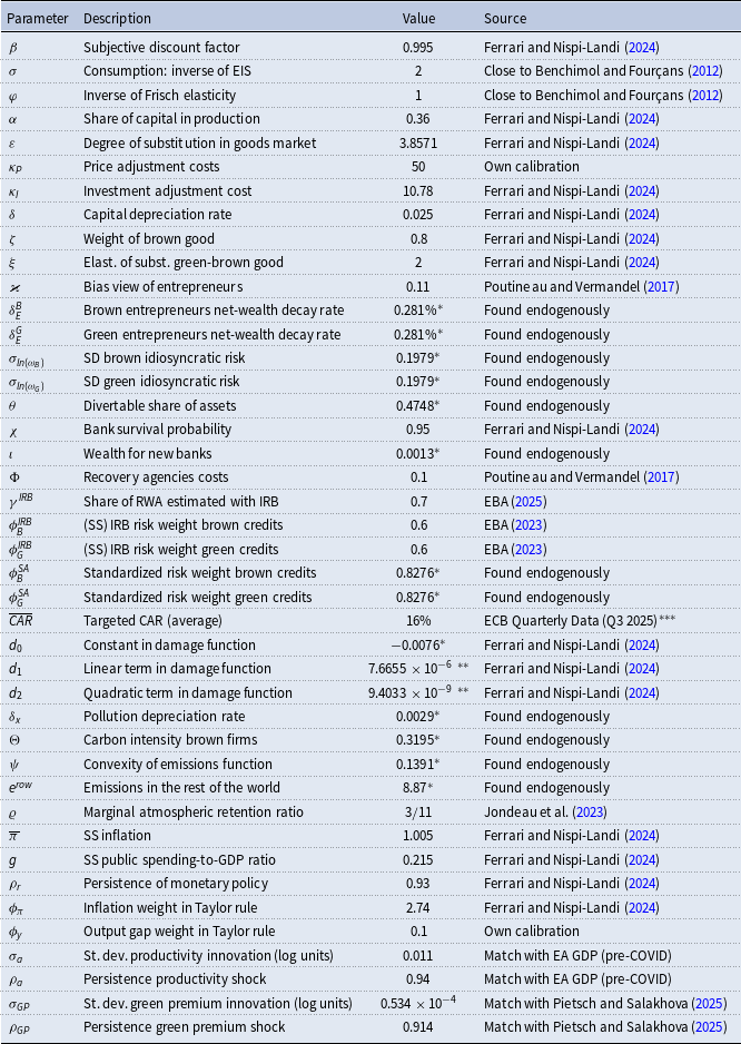

 CAR¯=16%
 1.11%
 0.534
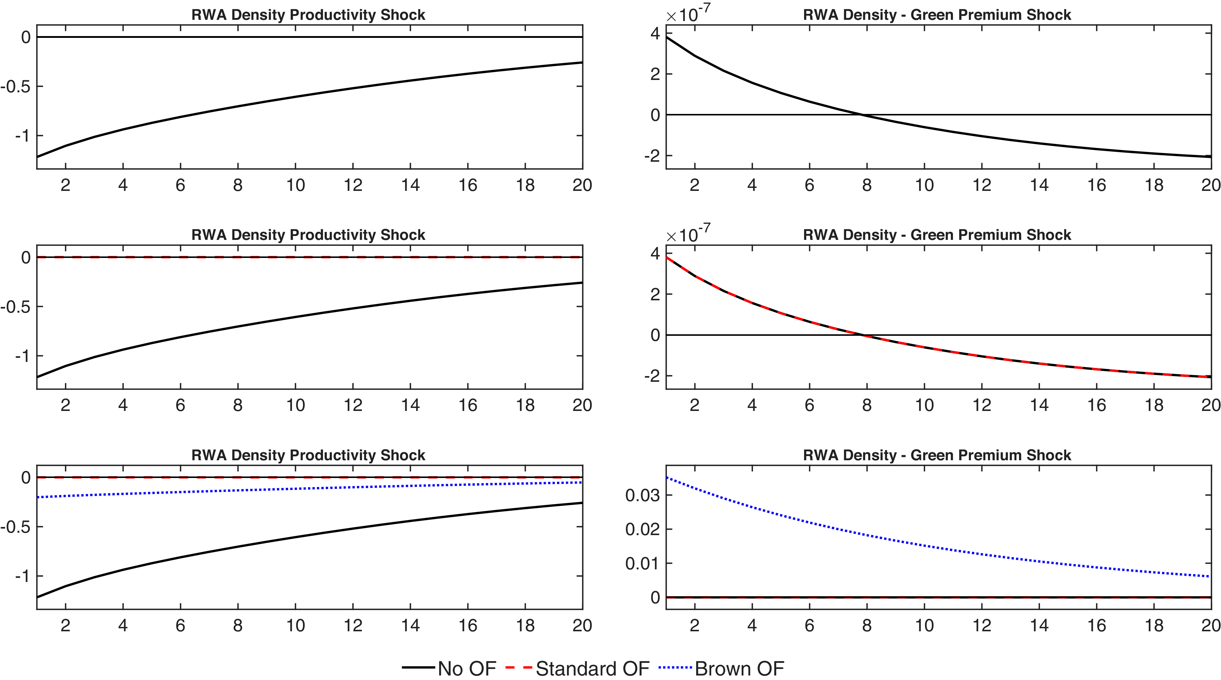
 1.11%
 0.534
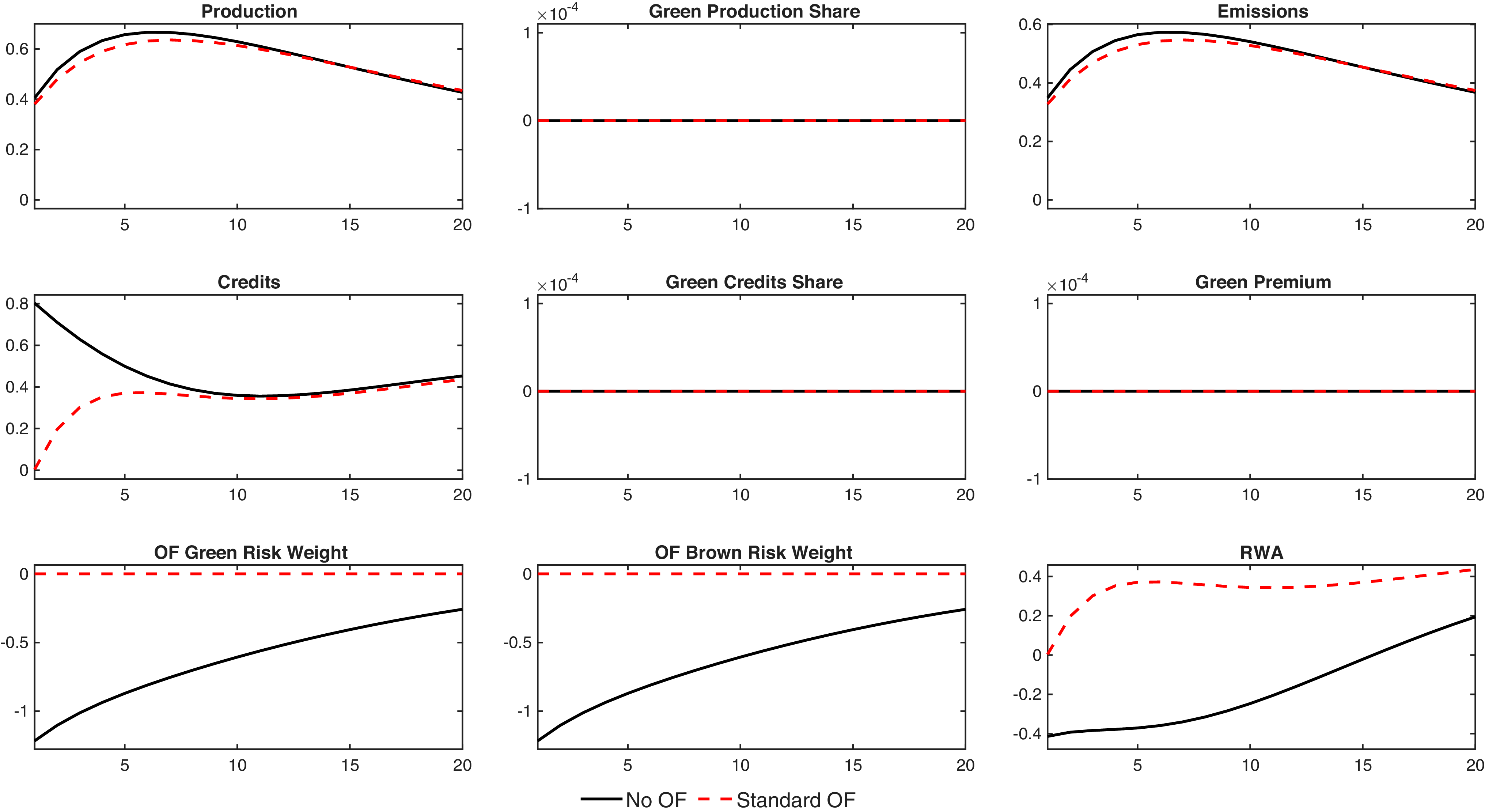
 x×10−6
 x×10−4
 1.11%

 x×10−6
 x×10−4
 0.534

 x×10−6
 x×10−4
 1.11%

 x×10−6
 x×10−4
 0.534
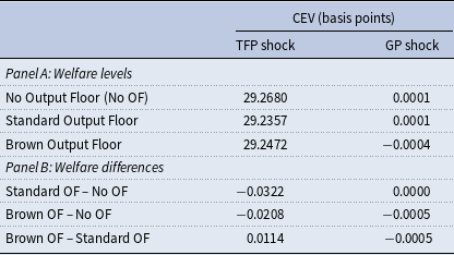
 =λp
 T=150
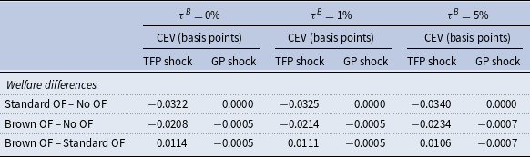
 =λp
 T=150
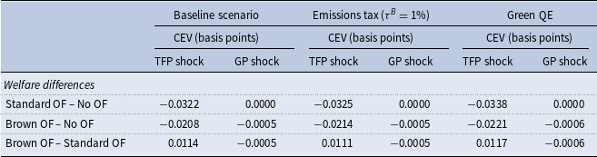
 =λp
 T=150

 CAR¯=16%
 1.11%
 0.534

 1.11%
 0.534



