What is already known?

• • Several freely available computational packages provide powerful and flexible tools for network meta-analysis. The multivariate meta-analysis and meta-regression frameworkReference Higgins, Jackson, Barrett, Lu, Ades and White ^{1 –} Reference White ³ provides a general frequentist formulation for evidence synthesis and inconsistency assessment.

What is new?

• • We developed NMA, an R package organized around the multivariate meta-analysis and meta-regression framework and designed to complement existing software.

• • The NMA package brings together a broad range of functions for evidence synthesis, heterogeneity and inconsistency assessment, comparative effectiveness analysis, and graphical visualization within a common analytical workflow.

• • Key analytical tools—including Higgins’ global inconsistency test, network meta-regression, and advanced inferential and prediction methods designed to improve uncertainty quantificationReference Noma, Hamura, Gosho and Furukawa ^{4 ,} Reference Noma, Hamura, Sugasawa and Furukawa ⁵ —are implemented.

• • Data-handling tools facilitate the integration of arm-level data and summary effect estimates, providing additional flexibility, particularly for survival outcomes.

Potential impact for RSM readers

• • The package facilitates the practical use of network meta-analysis for a broad range of researchers, including non-statisticians, thereby enhancing the accessibility of systematic reviews on important clinical and public health questions.

• • By comprehensively covering standard analyses and graphical tools, the NMA package is also valuable for educational purposes, serving as a practical resource for students, researchers, and clinicians to learn research methods through real-world case studies.

3.1. Functionalities and features

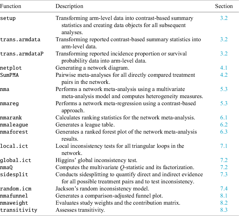
The R package NMA was developed as a collection of generic computational tools for network meta-analysis. It is based on the multivariate meta-regression framework proposed by White et al.Reference White, Barrett, Jackson and Higgins ² and is designed to apply effective statistical methods available within this model. Table 1 provides an overview of the functions implemented in the package.

Table 1.

Main functions of the NMA package and their descriptions

Table 1. Long description

The table consists of three columns: Function, Description, and Section.

* setup: Transforming arm-level data into contrast-based summary statistics and creating data objects for all subsequent analyses. Section 3.2.

* trans dot armdata: Transforming reported contrast-based summary statistics into arm-level data. Section 3.2.

* trans dot armdata P: Transforming reported incidence proportion or survival probability data into arm-level data. Section 3.2.

* netplot: Generating a network diagram. Section 4.1.

* Sum P M A: Pairwise meta-analyses for all directly compared treatment pairs in the network. Section 4.2.

* nma: Performs a network meta-analysis using a multivariate meta-analysis model and computes heterogeneity measures. Section 5.3.

* nmareg: Performs a network meta-regression using a contrast-based approach. Section 5.3.

* nmarank: Calculates ranking statistics for the network meta-analysis. Section 6.1.

* nmaleague: Generates a league table. Section 6.2.

* nmaforest: Generates a ranked forest plot of the network meta-analysis results. Section 6.3.

* local dot ict: Local inconsistency tests for all closed loops in the network. Section 7.1.

* global dot ict: Higgins’ global inconsistency test. Section 7.2.

* nma Q: Computes the multivariate Q-statistic and its factorization. Section 7.2.

* sidesplit: Conducts sidesplitting to quantify direct and indirect evidence for all possible treatment pairs and to test inconsistency. Section 7.3.

* random dot icm: Jackson’s random inconsistency model. Section 7.4.

* nmafunnel: Generates a comparison-adjusted funnel plot. Section 8.1.

* nmaweight: Evaluates study weights and the contribution matrix. Section 8.2.

* transitivity: Assesses transitivity. Section 8.3.

The package brings together a range of methods within the multivariate meta-regression framework, including network meta-regression, Higgins’s global inconsistency test, Jackson’s random inconsistency model,Reference Jackson, Barrett, Rice, White and Higgins ¹⁹ higher-order inference and prediction methods developed by Noma et al.,Reference Noma, Hamura, Gosho and Furukawa ^{4 ,} Reference Noma, Hamura, Sugasawa and Furukawa ⁵ and tools for assessing transitivity. In addition, the package offers data-handling tools that facilitate the integration of arm-based data (e.g., means, standard deviations) with trials reporting only contrast-based effect measures (e.g., mean differences).

To ensure accessibility for non-statisticians, the package has been designed with a user-friendly interface. Once an analysis dataset is generated using the setup function, all analytical tools can be applied with simple commands using the generated object. In the following sections, we provide an overview of the purpose of each function, how to use them, and how to interpret their results.

3.2. Supported data types and setup

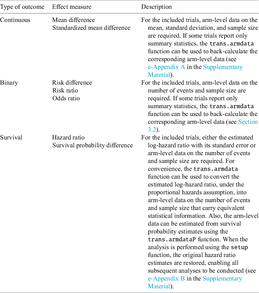
The NMA package accommodates three types of outcomes—continuous, binary, and survival—as summarized in Table 2. For each outcome type, the package enables estimation using several effect measures, including the mean difference, standardized mean difference, risk difference, risk ratio, odds ratio, hazard ratio, and survival probability difference.

Table 2.

Outcome types supported in the NMA package and their descriptions

Table 2. Long description

The table is organized into three columns: Type of outcome, Effect measure, and Description.

* Continuous: Effect measures include Mean difference and Standardized mean difference. Description: Requires arm-level data on mean, standard deviation, and sample size. The trans dot armdata function can back-calculate arm-level data from summary statistics.

* Binary: Effect measures include Risk difference, Risk ratio, and Odds ratio. Description: Requires arm-level data on the number of events and sample size. The trans dot armdata function can be used for back-calculation.

* Survival: Effect measures include Hazard ratio and Survival probability difference. Description: Requires either estimated log-hazard ratio with its standard error or arm-level data on events and sample size. The trans dot armdata function converts log-hazard ratios into arm-level data under proportional hazards assumptions. The trans dot armdata P function can estimate arm-level data from survival probability estimates.

All analyses require that data be prepared in the arm-level format. These arm-level datasets are edited by the setup function, which edits and creates contrast-based statistics suitable for the analyses using multivariate meta-analysis models. As in conventional meta-analysis, however, mixed data of arm-level and summary-level statistics are often created in practice.Reference Higgins, Thomas, Chandler, Cumpston, Li, Page and Welch ²⁴ The NMA package therefore provides dedicated functions for handling such cases. For example, in continuous outcomes, some trials may report mean, standard deviation, and sample size for each arm, whereas others provide only contrast-based effect measures such as the mean difference with a standard error (which can be reconstructed from confidence intervals or p-values). In the latter case, the function trans.armdata can be used to back-calculate (pseudo) arm-level data. Note that the reconstructed values will not necessarily reproduce the original arm-level data exactly. However, in practice, the setup function transforms all the (pseudo) arm-level data into contrast-based effect measures for analysis, and the resulting summary measures are designed to coincide closely with the originally reported effect measures. Thus, the arm-level data generated by trans.armdata should be viewed as “working” pseudo-data, serving as a bridge to construct contrast-based summaries.

For survival outcomes, hazard ratios are frequently reported.Reference Parmar, Torri and Stewart ²⁵ These summary data can also be passed to trans.armdata. Under the proportional hazards assumption, the function applies the complementary log–log transformation to invert the hazard ratio formula,Reference Hedeker, Siddiqui and Hu ^{26 ,} Reference Salika, Turner, Fisher, Tierney and White ²⁷ thereby generating pseudo-data in the form of reconstructed event counts. Also, arm-specific survival probability data can sometimes be obtained from a Kaplan–Meier plot.Reference Parmar, Torri and Stewart ²⁵ These survival probabilities can be converted into (pseudo) event counts and sample sizes using the trans.armdataP function. These pseudo-data can then be combined with trials reporting only event counts and sample sizes, producing a dichotomized arm-level dataset across all studies. Passing this dataset to the setup function yields contrast-based effect measures expressed as hazard ratios, which reproduce the original estimates.

Once arm-level data from different-type data are merged into a single dataset, the setup function can produce contrast-based effect measures. All subsequent analyses can then be performed using the resulting object with simple commands. If arm-level covariates are available—for example, summary baseline characteristics that can be used in meta-regression or for evaluating transitivity—these variables can be added directly to the dataset in advance. Such data editing may conveniently be carried out in spreadsheet software such as Microsoft Excel (Microsoft, Redmond, WA.).

As an illustrative example for the binary outcome case, the required variables include study identifier (study), treatment (trt), number of events (d), sample size (n), and covariates (z; optional, multiple allowed). Users must also specify the effect measure of interest (risk difference, risk ratio, or odds ratio) and designate a reference treatment (ref).

> hf2 <- setup(study=study,trt=trt,d=d,n=n,z=c(SBP,DBP,pubyear),
  measure="OR",ref="Placebo",data=heartfailure)

Using the output object generated by the setup function as an argument, all subsequent analyses can be executed with simple commands.

4.1. Network diagram

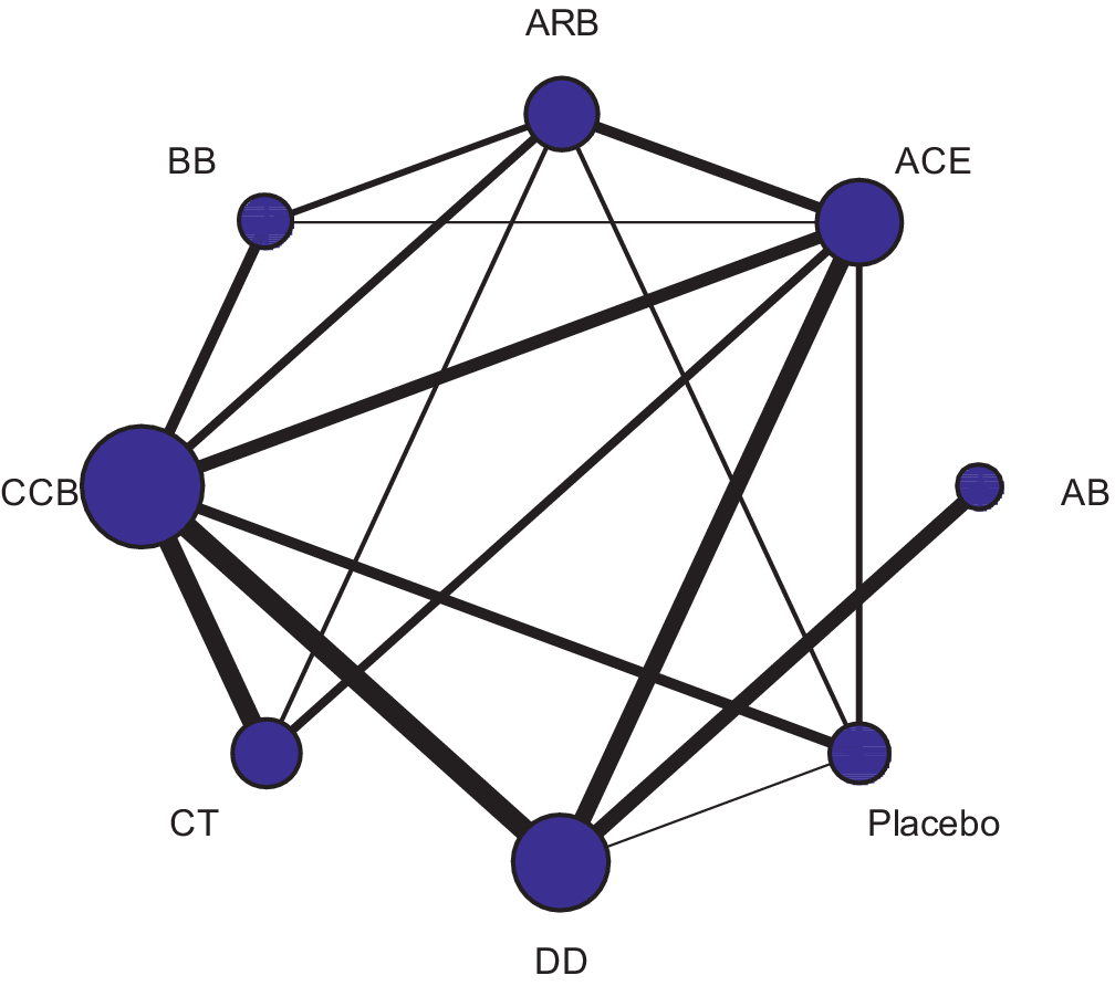
In network meta-analysis, network diagramsReference Hutton, Salanti and Caldwell ²⁸ are presented in most studies to visualize both the amount and structure of the evidence being synthesized. The NMA package facilitates this process through the netplot function, which enables users to generate such diagrams in a straightforward manner. The function can be executed using the syntax illustrated below, and its specifications can be flexibly modified according to user preferences. The size of the nodes and the thickness of the edges in the netplot function are proportional to the total sample size for each treatment and each direct comparison, respectively.

> netplot(hf2)

(The figure created is shown in Figure 1.)

Figure 1.

Network diagram of the antihypertensive drug study created using the netplot function.

Figure 1. Long description

The diagram consists of blue circular nodes of varying sizes arranged in a circular pattern, connected by black lines of varying thicknesses.

Starting from the top and moving clockwise, the nodes are labeled:

* A R B at the 12 o'clock position.

* A C E at the 2 o'clock position.

* A B positioned slightly outside the main circle at the 3 o'clock position.

* Placebo at the 5 o'clock position.

* D D at the 6 o'clock position.

* C T at the 7 o'clock position.

* C C B at the 9 o'clock position.

* B B at the 11 o'clock position.

Node sizes indicate volume, with C C B being the largest, followed by A C E and D D. B B and A B are the smallest nodes.

Line thickness represents the strength or frequency of connections:

* The thickest lines connect C C B to A C E, C C B to D D, and A C E to D D.

* Moderately thick lines connect C C B to C T, C C B to B B, A C E to Placebo, and A B to Placebo.

* Thin lines connect A R B to A C E, B B, C C B, and D D.

* A thin line also connects Placebo to D D and A C E.

4.2. Pairwise meta-analysis for all treatment pairs with direct comparisons

As part of the basic information, the results of pairwise meta-analyses for all direct comparisons in the network can be summarized using the SumPMA function. This output includes the results of meta-analyses based on the DerSimonian–Laird-type random-effects model,Reference DerSimonian and Laird ²⁹ along with estimates of τ ², I ², and H ² statistics, and Egger’s test.Reference Egger, Davey Smith, Schneider and Minder ³⁰ By default, the restricted maximum likelihood (REML) method is adopted.

> SumPMA(hf2)
Coding:
 code treatment
    1   Placebo
    2        AB
    3       ACE
    4       ARB
    5        BB
    6       CCB
    7        CT
    8        DD

Summary effect measures:
        N Estimate Lower Upper Pr(>|z|)
1 vs. 3 1    0.759 0.663 0.869    0.000
1 vs. 4 2    0.845 0.547 1.304    0.447
1 vs. 6 3    0.678 0.485 0.949    0.023
1 vs. 8 1    0.375 0.228 0.615    0.000
2 vs. 8 1    0.494 0.433 0.564    0.000
3 vs. 4 1    1.052 0.929 1.192    0.424
3 vs. 5 1    0.834 0.347 2.003    0.684
3 vs. 6 3    1.189 1.076 1.314    0.001
3 vs. 7 1    0.878 0.630 1.225    0.445
3 vs. 8 1    1.136 0.818 1.577    0.447
4 vs. 5 1    1.058 0.845 1.325    0.622
4 vs. 6 1    1.145 0.989 1.326    0.070
4 vs. 7 2    1.501 0.991 2.272    0.055
5 vs. 6 1    0.839 0.665 1.057    0.137
6 vs. 7 3    0.865 0.743 1.007    0.061
6 vs. 8 5    0.711 0.644 0.786    0.000

Heterogeneity measures:
        N   tau tau^2   I^2   H^2
1 vs. 3 1 0.000 0.000 0.000 1.000
1 vs. 4 2 0.281 0.079 0.806 5.157
1 vs. 6 3 0.000 0.000 0.000 1.000
1 vs. 8 1 0.000 0.000 0.000 1.000
2 vs. 8 1 0.000 0.000 0.000 1.000
3 vs. 4 1 0.000 0.000 0.000 1.000
3 vs. 5 1 0.000 0.000 0.000 1.000
3 vs. 6 3 0.000 0.000 0.000 1.000
3 vs. 7 1 0.000 0.000 0.000 1.000
3 vs. 8 1 0.000 0.000 0.000 1.000
4 vs. 5 1 0.000 0.000 0.000 1.000
4 vs. 6 1 0.000 0.000 0.000 1.000
4 vs. 7 2 0.152 0.023 0.253 1.339
5 vs. 6 1 0.000 0.000 0.000 1.000
6 vs. 7 3 0.000 0.000 0.000 1.000
6 vs. 8 5 0.001 0.000 0.000 1.000

5.1. Multivariate meta-analysis models and synthesis methods

The contrast-based approach is one of the principal methods used for evidence synthesis in network meta-analysis.Reference Salanti ^{22 ,} Reference Lu and Ades ³¹ In this framework, effect measures such as odds ratios, hazard ratios, or mean differences are modeled as outcome measures. This approach can be interpreted as a generalization of the conventional DerSimonian–Laird method for pairwise meta-analysis,Reference DerSimonian and Laird ²⁹ whereby study-specific outcomes are treated as multivariate outcomes and modeled within a multivariate meta-analysis framework.Reference Jackson, Riley and White ³²

White et al.Reference White, Barrett, Jackson and Higgins ² demonstrated that such multivariate meta-regression models allow for the implementation of contrast-based network meta-analysis, and further showed that this framework provides a general means to evaluate inconsistency through the design-by-treatment interaction model.Reference Higgins, Jackson, Barrett, Lu, Ades and White ¹ In this section, we outline the underlying statistical model and corresponding analytical procedures.

Specifically, we consider the synthesis of $N$ trials comparing $p+1$ treatments. Let ${Y}_{ij}$ denote the estimator of the treatment effect of the jth treatment relative to a designated reference treatment (e.g., placebo) in the ith trial $\left(i=1,2,\dots, N;j=1,2,\dots, p\right)$ . Commonly used effect measures include the mean difference, standardized mean difference, risk difference, risk ratio, odds ratio, and hazard ratio, with ratio measures typically modeled on the logarithmic scale. For the contrast-based network meta-regression, we adopt a multivariate meta-analysis model for the outcome variable ${\boldsymbol{Y}}_i={\left({Y}_{i1},{Y}_{i2},\dots, {Y}_{ip}\right)}^T$ ,

(*) $$\begin{align}{\boldsymbol{Y}}_i={\boldsymbol{\theta}}_i+{\boldsymbol{e}}_i \quad\end{align}$$

$$\begin{align*}{\boldsymbol{\theta}}_i={\boldsymbol{X}}_i^T\boldsymbol{\beta} +{\boldsymbol{\varepsilon}}_i,\end{align*}$$

where ${\boldsymbol{\theta}}_i={\left({\theta}_{i1},{\theta}_{i2},\dots, {\theta}_{ip}\right)}^T$ and $\boldsymbol{\beta} ={\left({\boldsymbol{\beta}}_1^T,\dots, {\boldsymbol{\beta}}_p^T\right)}^T$ . The regression function model ${\boldsymbol{X}}_i^T\boldsymbol{\beta}$ involves a design matrix,

$$\begin{align*}{\boldsymbol{X}}_i=\left(\begin{array}{cccc}{\boldsymbol{x}}_{i1}& 0& \cdots & 0\\ {}0& {\boldsymbol{x}}_{i2}& \dots & 0\\ {}\vdots & \vdots & \ddots & \vdots \\ {}0& 0& \cdots & {\boldsymbol{x}}_{ip}\end{array}\right),\end{align*}$$

where ${\boldsymbol{x}}_{ij}$ is a ${q}_j\times 1$ covariate vector for ${Y}_{ij}$ ( ${q}_j$ is the number of the covariates) and ${\boldsymbol{\beta}}_j$ is its ${q}_j\times 1$ regression coefficient vector. Also, ${\boldsymbol{e}}_i$ and ${\boldsymbol{\varepsilon}}_i$ are independent random variation terms within and across studies ( $p\times 1$ random vectors), assumed to be distributed ${\boldsymbol{e}}_i\sim \mathrm{MVN}\left(\boldsymbol{0},{\boldsymbol{S}}_i\right)\kern0.24em \mathrm{and}\;{\boldsymbol{\varepsilon}}_i\sim \mathrm{MVN}\left(\boldsymbol{0},\boldsymbol{\Sigma} \right)$ . ${\boldsymbol{S}}_i$ (a $p\times p$ matrix) is the within-study covariance matrix,

$$\begin{align*}{\boldsymbol{S}}_i=\left(\begin{array}{cccc}{s}_{i1}^2& {\rho}_{i12}{s}_{i1}{s}_{i2}& \cdots & {\rho}_{i1p}{s}_{i1}{s}_{ip}\\ {}{\rho}_{i21}{s}_{i2}{s}_{i1}& {s}_{i2}^2& \dots & {\rho}_{i2p}{s}_{i2}{s}_{ip}\\ {}\vdots & \vdots & \ddots & \vdots \\ {}{\rho}_{ip1}{s}_{ip}{s}_{i1}& {\rho}_{ip2}{s}_{ip}{s}_{i2}& \cdots & {s}_{ip}^2\end{array}\right),\end{align*}$$

which is usually assumed to be known and fixed to its valid estimate.Reference Noma ³³ In addition, $\boldsymbol{\Sigma}$ is the between-studies variance–covariance matrix:

$$\begin{align*}\boldsymbol{\Sigma} ={\tau}^2\boldsymbol{P}={\tau}^2\left(\begin{array}{cccc}1& 1/2& \cdots & 1/2\\ {}1/2& 1& \dots & 1/2\\ {}\vdots & \vdots & \ddots & \vdots \\ {}1/2& 1/2& \cdots & 1\end{array}\right)\end{align*}$$

for ${\tau}^2>0$ . Note that the correlation structure of $\boldsymbol{\Sigma}$ can be assumed to be unstructured; however, there are rarely enough studies to allow identification of all variance–covariance parameters. Consequently, most network meta-analyses adopt the equal-variance assumption for the p components of ${\boldsymbol{\varepsilon}}_i$ . Under this assumption, and by virtue of the consistency property, all pairwise correlation coefficients are set to 0.50.Reference Higgins and Whitehead ³⁴ In the NMA package, we likewise adopt the equal-variance assumption as the standard specification of the model.

For trials that do not include a reference treatment, the data augmentation strategy proposed by White et al.Reference White, Barrett, Jackson and Higgins ² can be applied; in this approach, a quasi-negligible dataset is added to the reference arm (e.g., 0.001 events for 0.01 patients in the case of a binary outcome). In addition, because most individual clinical trials typically involve only two to four arms, we formally employ subvectors or submatrices in the likelihood function.Reference White, Barrett, Jackson and Higgins ²

Standard network meta-analysis without covariates and under the consistency assumption can be expressed as a special case of the model with ${\boldsymbol{x}}_{ij}=\left(\boldsymbol{1}\right)$ , a vector of ones. Meta-regression analyses incorporating covariates can then be performed within the same framework. In terms of the classification by Donegan et al.,Reference Donegan, Dias, Tudur-Smith, Marinho and Welton ³⁵ the multivariate meta-regression model based on the framework proposed by White et al.Reference White, Barrett, Jackson and Higgins ² corresponds to the independent interaction assumption, in which treatment-by-covariate interaction coefficients may differ across treatment comparisons. Accordingly, the regression function is modeled separately for each outcome component. Furthermore, when ${\tau}^2=0$ , the model reduces to a fixed-effect model. In the NMA package, standard network meta-analyses can be conducted using the nma function, while meta-regression can be performed with the nmareg function.

Model parameters can be estimated using the standard REML method. Under a random-effects model, as in pairwise meta-analyses, the confidence intervals for $\boldsymbol{\beta}$ may be inaccurate when the number of studies N is small.Reference Noma, Hamura, Gosho and Furukawa ^{4 ,} Reference Noma, Nagashima, Maruo, Gosho and Furukawa ^{18 ,} Reference Partlett and Riley ³⁶ The Cochrane HandbookReference Higgins, Thomas, Chandler, Cumpston, Li, Page and Welch ²⁴ recommends the use of the Hartung–Knapp–Sidik–Jonkman (HKSJ) methodReference IntHout, Ioannidis and Borm ^{17 ,} Reference Hartung and Knapp ^{37 ,} Reference Sidik and Jonkman ³⁸ for pairwise meta-analyses. For network meta-analysis, Noma et al.Reference Noma, Hamura, Gosho and Furukawa ⁴ also proposed a higher-order asymptotic correction, which has been adopted as the default method in the NMA package.

5.2. Assessment of heterogeneity

The issue of between-trial heterogeneity in treatment effects is also of central importance in network meta-analysis. The conventional measures used in pairwise meta-analysis, such as Cochran’s Q-testReference Cochran ³⁹ and Higgins’ I ² statistic,Reference Higgins and Thompson ⁴⁰ have been extended to the multivariate meta-analysis framework by Jackson et al.,Reference Jackson, White and Riley ²¹ and can be directly computed from model (*). The parameter $\tau$ can be interpreted as the heterogeneity standard deviation. In addition, prediction intervals,Reference Higgins, Thompson and Spiegelhalter ⁴¹ which represent the expected range of treatment effects in future populations while accounting for between-study heterogeneity, have become widely used in recent meta-analyses. Although prediction intervals have commonly been calculated using approximations based on the t-distribution, concerns about their accuracy have been raised.Reference Partlett and Riley ^{36 ,} Reference Nagashima, Noma and Furukawa ⁴² To address this issue, Noma et al.Reference Noma, Hamura, Sugasawa and Furukawa ⁵ proposed several improved methods. The NMA package adopts, as the default method, an approach based on higher-order asymptotic approximations developed by Noma et al.,Reference Noma, Hamura, Sugasawa and Furukawa ⁵ and these results are reported collectively in the output of the nma function.

5.3. Computational tools for primary synthesis methods

The synthesis analysis based on the consistency assumption can be performed by the nma function, which adopts the higher-order asymptotic correction methods proposed by Noma et al.Reference Noma, Hamura, Gosho and Furukawa ^{4 ,} Reference Noma, Hamura, Sugasawa and Furukawa ⁵ as default (named as “Noma-Hamura” methods). The output also provides various heterogeneity statistics, including $\tau$ , ${\tau}^2$ , the ${H}^2$ statistic, the ${I}^2$ statistic, the Q-test, and the prediction interval. By setting eform=TRUE, the estimated effect measures are exponentiated, thereby allowing direct interpretation of effect sizes such as odds ratios, risk ratios, and hazard ratios, which are synthesized on the logarithmic scale under normality assumptions.

> nma(hf2, eform=TRUE)
Coding:
 code treatment
    1   Placebo
    2        AB
    3       ACE
    4       ARB
    5        BB
    6       CCB
    7        CT
    8        DD
    
Reference: Placebo

Number of studies: 26

Method: Noma-Hamura's improved REML-based inference and prediction
methods

Coef. (vs. treat 1):
         Est.    SE Lower Upper Pr(>|z|)
2: cons 1.214 0.165 0.811 1.818    0.284
3: cons 0.714 0.086 0.586 0.870    0.004
4: cons 0.759 0.088 0.626 0.919    0.009
5: cons 0.878 0.133 0.659 1.170    0.345
6: cons 0.843 0.093 0.689 1.033    0.092
7: cons 0.775 0.112 0.611 0.982    0.037
8: cons 0.600 0.113 0.465 0.774    0.001

tau (Between-studies_SD) estimate: 0.099

tau2 (Between-studies_variance) estimate: 0.01

Multivariate H2-statistic: 1.604

Multivariate I2-statistic: 0.594

Test for Heterogeneity: Q(df = 21) = 33.688, p-value = 0.039

95%PI (vs. treat 1):
        Lower Upper
2: cons 0.741 1.990
3: cons 0.525 0.972
4: cons 0.566 1.016
5: cons 0.612 1.258
6: cons 0.626 1.136
7: cons 0.563 1.065
8: cons 0.425 0.847

Similarly, network meta-regression can be conducted using the nmareg function. The example below illustrates an analysis of effect modification for the odds ratio of ACE versus placebo with systolic blood pressure (SBP) included as a covariate. It should be noted that in multivariate meta-regression, a different regression function is specified for each component of the outcome vectors ${\boldsymbol{Y}}_1,\dots, {\boldsymbol{Y}}_N$ . The variable to be evaluated as an effect modifier is specified via the argument z, and the corresponding outcome components are designated using the argument treats. For instance, to perform a meta-regression analysis assessing effect modification of SBP on the odds ratio for treatment 3 versus 1, the following command can be applied. Both z and treats can be specified as vectors to allow for the inclusion of multiple covariates and outcomes.

> nmareg(hf2,z=SBP,treats=3)
Covariates: SBP

Outcomes evaluated the effect modifications: 3 vs. 1

Coefficients:
         Coef.    SE  Lower  Upper Pr(>|z|)
2: cons  0.170 0.165 -0.154  0.493    0.304
3: cons  0.141 0.468 -0.776  1.058    0.763
3: SBP  -0.003 0.003 -0.009  0.003    0.297
4: cons -0.288 0.087 -0.459 -0.118    0.001
5: cons -0.154 0.134 -0.417  0.109    0.250
6: cons -0.203 0.095 -0.389 -0.017    0.032
7: cons -0.306 0.120 -0.540 -0.071    0.011
8: cons -0.535 0.110 -0.751 -0.319    0.000

Between-studies SD: 0.102

In addition, estimation of the regression coefficients requires sufficient information and covariate variation in the network to identify the specified meta-regression model. Because the multivariate meta-regression model combines information across the network, identifiability is not determined solely by the number of trials directly comparing the corresponding treatment pair. If the specified model is not identifiable from the available network evidence, estimation will fail and an error will be produced.

6.1. Ranking probability and SUCRA

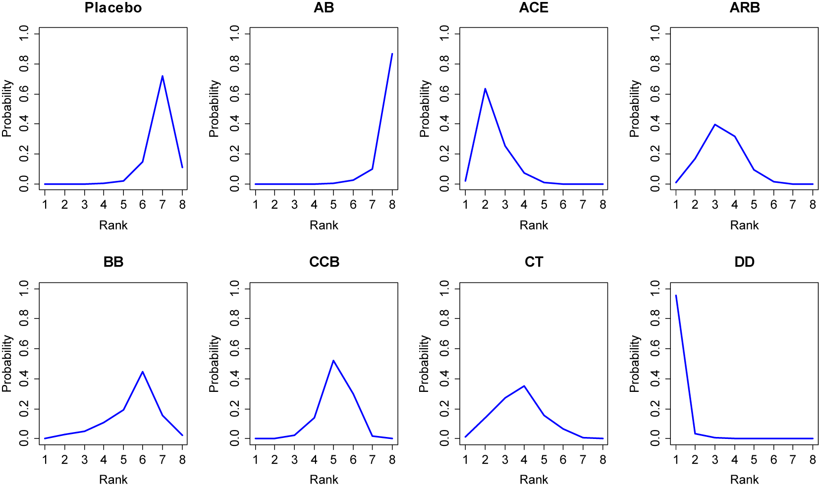
As an analytic approach to comparative effectiveness, treatment ranking methods are widely used.Reference Salanti ²² Based on the estimates from model (*), the probabilities of each treatment being ranked best, second, …, or worst can be estimated using a parametric bootstrap procedure.Reference Chaimani, Higgins, Mavridis, Spyridonos and Salanti ⁴³ In addition, the bootstrap method can be used to estimate the surface under the cumulative ranking curve (SUCRA).Reference Salanti, Ades and Ioannidis ⁴⁴ SUCRA is a continuous score ranging from 0 to 1 that indicates the relative position of each treatment within the overall distribution (analogous to a quantile of the distribution). These quantities can be computed using the nmarank function, which also provides plots of the ranking probabilities.

> nmarank(hf2)
SUCRA:
        SUCRA
DD      0.992
ACE     0.796
ARB     0.660
CT      0.612
CCB     0.407
BB      0.354
Placebo 0.155
AB      0.025

(The ranking probabilities of each treatment are presented in Figure 2.)

Figure 2.

Ranking probability plot of the antihypertensive drug study created using the nmarank function.

Figure 2. Long description

The figure consists of eight individual line graphs. Each graph shares a common X-axis labeled Rank from 1 to 8 and a Y-axis labeled Probability from 0.0 to 1.0.

Top Row from left to right:

* Placebo: The curve remains near zero until rank 5, then rises sharply to a peak of approximately 0.7 at rank 7 before dropping.

* A B: The curve stays at zero until rank 6, then shows an exponential increase, reaching its highest point of nearly 0.9 at rank 8.

* A C E: The curve rises immediately from rank 1 to a peak of 0.6 at rank 2, then follows an asymptotic decay toward zero by rank 6.

* A R B: The curve rises to a broad peak of 0.4 at rank 3 and 4, then gradually declines to zero by rank 7.

Bottom Row from left to right:

* B B: The curve shows a gradual linear increase from rank 1, peaking at 0.45 at rank 6, then declining.

* C C B: The curve remains low until rank 3, rises to a peak of 0.5 at rank 5, and drops back to zero by rank 8.

* C T: The curve shows a bell-shaped distribution peaking at 0.35 at rank 4.

* D D: The curve starts at its maximum of nearly 1.0 at rank 1 and drops immediately to near zero by rank 2, remaining flat for the rest of the ranks.

6.2. League table

As another type of output for comparative effectiveness, a league tableReference Salanti, Ades and Ioannidis ⁴⁴ can also be generated easily using the nmaleague function. The league table can additionally be exported in CSV format.

Based on the results of the synthesis analysis, a league table can be created with user-specified options. The number of decimal places can be set via the argument digits, and the output file name for CSV export can be specified using out.csv. For example:

> nmaleague(hf2, eform=TRUE, digits=2, out.csv="nmaleague_out.csv")

(The output is omitted here due to space limitations.)

6.3. Ranked forest plot

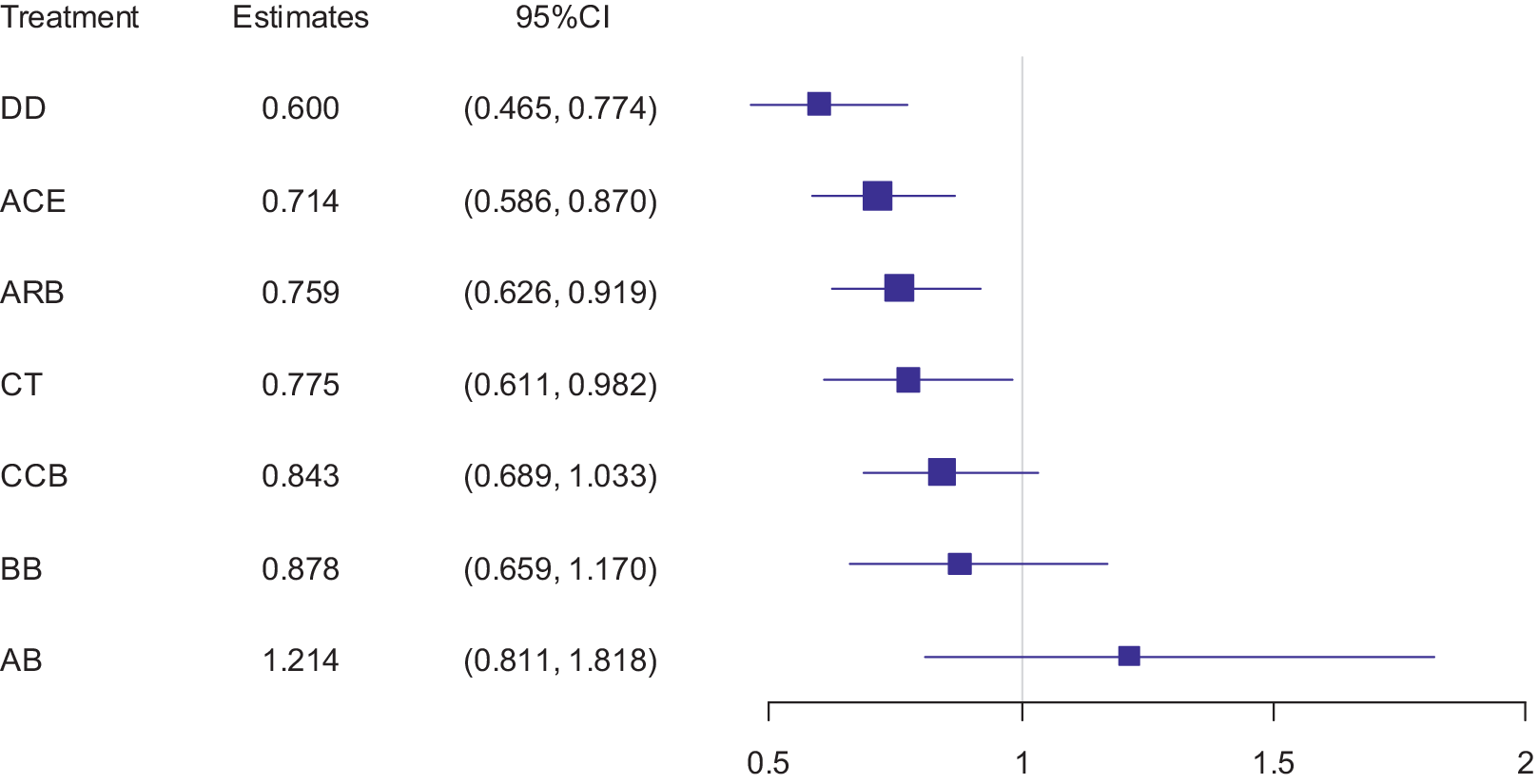
The results of the synthesis analysis are often presented graphically using a forest plot. For comparative effectiveness analyses, a ranked forest plot,Reference Nikolakopoulou, Higgins and Papakonstantinou ⁴⁵ in which treatments are ordered by their estimated effect measures, is frequently employed. Such plots can be easily generated using the nmaforest function.

> nmaforest(hf2, col.plot="blue")

(The forest plot created is shown in Figure 3.)

Figure 3.

Ranked forest plot of the antihypertensive drug study created using the nmaforest function.

Figure 3. Long description

The forest plot is organized into four columns: Treatment, Estimates, 95% C I, and a graphical representation. A vertical line of null effect is positioned at 1 on the x-axis, which ranges from 0.5 to 2.

From top to bottom, the data rows are:

* D D: Estimate 0.600, 95% C I 0.465 to 0.774. The square and error bars are entirely to the left of the null line.

* A C E: Estimate 0.714, 95% C I 0.586 to 0.870. Positioned to the left of the null line.

* A R B: Estimate 0.759, 95% C I 0.626 to 0.919. Positioned to the left of the null line.

* C T: Estimate 0.775, 95% C I 0.611 to 0.982. Positioned to the left of the null line.

* C C B: Estimate 0.843, 95% C I 0.689 to 1.033. The error bars cross the null line.

* B B: Estimate 0.878, 95% C I 0.659 to 1.170. The error bars cross the null line.

* A B: Estimate 1.214, 95% C I 0.811 to 1.818. The square is to the right of the null line, with error bars crossing it.

The treatments are ranked in ascending order of their point estimates.

7.1. Local inconsistency test

Various statistical methods have been proposed for evaluating inconsistency, and several representative approaches are implemented in the NMA package. The first is the local inconsistency test (local.ict function). This method extracts triangular loops of three treatments from the evidence network and tests whether the treatment effects obtained from the direct and indirect comparison paths within each loop are consistent.Reference Veroniki, Vasiliadis, Higgins and Salanti ^{46 ,} Reference Bucher, Guyatt, Griffith and Walter ⁴⁷

> local.ict(hf2)
Local inconsistency tests:
            N   tau X2-statistic df Pr(>X2)
loop: 1-3-4 4 0.281        0.015  1  0.903
loop: 1-3-6 7 0.007        2.218  1  0.136
loop: 1-3-8 4 0.179        2.627  1  0.105
loop: 1-4-6 6 0.203        1.161  1  0.281
loop: 1-6-8 9 0.009        0.664  1  0.415
loop: 3-4-5 3 0.009        0.385  1  0.535
loop: 3-4-6 5 0.008        0.015  1  0.903
loop: 3-4-7 5 0.163        1.644  1  0.200
loop: 3-5-6 5 0.007        1.301  1  0.254
loop: 3-6-7 6 0.008        3.304  3  0.347
loop: 3-6-8 8 0.006        3.538  3  0.316
loop: 4-5-6 3 0.007        1.978  1  0.160
loop: 4-6-7 6 0.009        3.669  1  0.055

7.2. Global inconsistency test

The second method is the global inconsistency test (global.ict function). While inconsistency within a triangular loop can be readily understood as the discrepancy between direct and indirect comparisons along the loop, it is less straightforward to define inconsistency across more complex networks. Higgins et al.Reference Higgins, Jackson, Barrett, Lu, Ades and White ¹ formalized this by defining inconsistency as “differences in treatment effects depending on which treatments are being compared,” and expressed it through a design-by-treatment interaction framework (where “design” refers to the set of treatments being compared).Reference Jackson, Boddington and White ⁴⁸ In this approach, all possible design-by-treatment interactions in the network are modeled within a meta-regression framework, and a test of the global null hypothesis regarding these interactions was proposed as the global inconsistency test.

> global.ict(hf2)
Coefficients of the design-by-treatment interaction model:
               Est.    SE  Lower  Upper Pr(>|z|)
2: cons      -0.277 0.343 -0.948  0.395    0.420
3: cons      -0.276 0.171 -0.610  0.059    0.106
4: cons      -0.160 0.147 -0.448  0.129    0.278
4: des_3-4   -0.065 0.281 -0.617  0.486    0.816
5: cons      -0.458 0.503 -1.444  0.529    0.363
5: des_4-5    0.355 0.559 -0.741  1.451    0.526
6: cons      -0.401 0.201 -0.795 -0.007    0.046
6: des_3-6    0.312 0.685 -1.031  1.654    0.649
6: des_3-6-7  0.370 0.327 -0.272  1.011    0.259
6: des_3-6-8  0.280 0.312 -0.331  0.891    0.369
6: des_4-6    0.377 0.303 -0.217  0.972    0.214
6: des_5-6   -0.233 0.576 -1.362  0.897    0.687
7: cons      -0.094 0.259 -0.601  0.413    0.717
7: des_3-7   -0.312 0.302 -0.903  0.280    0.302
7: des_4-7    0.341 0.366 -0.377  1.058    0.352
7: des_6-7   -0.530 0.363 -1.242  0.183    0.145
8: cons      -0.982 0.297 -1.565 -0.399    0.001
8: des_3-6-8  0.525 0.381 -0.222  1.271    0.168
8: des_3-8    0.833 0.412  0.025  1.641    0.043
8: des_6-8    0.156 0.438 -0.703  1.015    0.722

Between-studies SD: 0.156

P-value: 0.459

As a supplementary tool, the nmaQ function can be used to decompose the Q-statistic, providing Q-statistics for each design and separating the within-design and between-design components. This allows the results of heterogeneity tests to be obtained for each component.

> nmaQ(hf2)
Within designs (individual designs):
      N     n     Q df Pr(>Q)
1-3   1  9297 0.000  0  1.000
1-4   2  7439 5.157  1  0.023
1-6   3 16800 0.502  2  0.778
1-8   1  3845 0.000  0  1.000
2-8   1 24335 0.000  0  1.000
3-4   1 17118 0.000  0  1.000
3-5   1   758 0.000  0  1.000
3-6   1   470 0.000  0  1.000
3-6-7 1  6614 0.000  0  1.000
3-6-8 1 33357 0.000  0  1.000
3-7   1 10985 0.000  0  1.000
3-8   1  6083 0.000  0  1.000
4-5   1  9193 0.000  0  1.000
4-6   1 15245 0.000  0  1.000
4-7   2  5129 1.339  1  0.247
5-6   1 19257 0.000  0  1.000
6-7   2 27357 0.074  1  0.786
6-8   4 10031 4.581  3  0.205

Q-statistics:
                     Q df Pr(>Q)
Within designs  11.652  8  0.167
Between designs 22.036 13  0.055
Total           33.688 21  0.039

7.3. Sidesplitting

The third method is side-splitting (sidesplit function). This approach summarizes the direct and indirect evidence for a specific pair of treatments and tests whether their pooled quantities are in disagreement. When multi-arm trials with three or more arms are included, special considerations are required to avoid bias.Reference Noma ^{49 ,} Reference Noma, Tanaka, Matsui, Cipriani and Furukawa ⁵⁰ The NMA package adopts the approach proposed by Noma,Reference Noma ⁴⁹ which is based on network meta-regression.

> sidesplit(hf2)
Direct evidence:
          Est.    SE  Lower  Upper Pr(>|z|)
1 vs. 3 -0.276 0.143 -0.556  0.005    0.054
1 vs. 4 -0.155 0.131 -0.411  0.101    0.234
1 vs. 6 -0.392 0.180 -0.744 -0.040    0.029
1 vs. 8 -0.982 0.261 -1.493 -0.471    0.000

Indirect evidence:
          Est.    SE  Lower  Upper Pr(>|z|)
1 vs. 3 -0.407 0.126 -0.654 -0.160    0.001
1 vs. 4 -0.440 0.137 -0.708 -0.172    0.001
1 vs. 6 -0.100 0.092 -0.280  0.081    0.278
1 vs. 8 -0.428 0.093 -0.611 -0.245    0.000

Difference between direct and indirect evidence with inconsistency test:
          Est.    SE  Lower  Upper Pr(>|z|)
1 vs. 3  0.131 0.191 -0.242  0.505    0.491
1 vs. 4  0.284 0.189 -0.086  0.655    0.133
1 vs. 6 -0.292 0.202 -0.688  0.103    0.148
1 vs. 8 -0.554 0.277 -1.097 -0.011    0.045

(Due to space limitations, only the top four rows of results are presented.)

7.4. Random inconsistency model

The fourth method is the random inconsistency model proposed by Jackson et al.Reference Jackson, Barrett, Rice, White and Higgins ¹⁹ (random.icm function). This approach extends the design-by-treatment interaction meta-regression model of Higgins et al.Reference Higgins, Jackson, Barrett, Lu, Ades and White ¹ by treating the design effects as random effects.Reference Jackson, Barrett, Rice, White and Higgins ^{19 ,} Reference Law, Jackson, Turner, Rhodes and Viechtbauer ²⁰ In this model, inconsistency can be evaluated by testing the variance component associated with the random design effects. In addition, this model provides I ² statistics for heterogeneity, for inconsistency, and for the overall model that jointly accounts for both heterogeneity and inconsistency.

> random.icm(hf2)
Number of designs: 18

Coef. (vs. treat 1):
         Coef.    SE  95%CL  95%CU P-value
2: cons  0.188 0.169 -0.144  0.519   0.267
3: cons -0.342 0.088 -0.514 -0.171   0.000
4: cons -0.283 0.091 -0.461 -0.106   0.002
5: cons -0.139 0.136 -0.406  0.129   0.310
6: cons -0.177 0.094 -0.360  0.006   0.058
7: cons -0.260 0.114 -0.483 -0.036   0.023
8: cons -0.517 0.112 -0.736 -0.299   0.000

Between-studies SD: 0.092

Between-designs SD: 0.055

Likelihood ratio tests for the variance components:
                              X2-statistic df P-value
Heterogeneity                        0.479  1   0.489
Inconsistency                        0.039  1   0.843
Heterogeneity + Inconsistency        0.519  2   0.772

Heterogeneity and inconsistency statistics:
                            R-statistic I2-statistic
Heterogeneity                     1.523        0.569
Inconsistency                     1.051        0.095
Heterogeneity + Inconsistency     1.602        0.610

8.1. Comparison-adjusted funnel plot

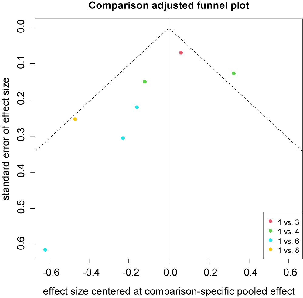
In network meta-analysis, the assessment of publication bias is challenging because multiple treatments are compared and the direction of publication bias may differ across trials. One approach is the comparison-adjusted funnel plot,Reference Chaimani, Higgins, Mavridis, Spyridonos and Salanti ⁴³ in which the results of trials with direct comparisons against a specified reference treatment are adjusted to share a common center line, thereby allowing a descriptive evaluation of publication bias across the network. Such plots can be generated using the nmafunnel function.

> nmafunnel(hf2,legends="bottomright")

(The comparison-adjusted funnel plot created is shown in Figure 4.)

Figure 4.

Comparison-adjusted funnel plot of the antihypertensive drug study created using the nmafunnel function.

Figure 4. Long description

A scatter plot with a vertical line at 0.0 on the x-axis and a dashed inverted V-shape forming a funnel.

* The x-axis is labeled effect size centered at comparison-specific pooled effect, ranging from -0.6 to 0.6.

* The y-axis is labeled standard error of effect size, ranging from 0.0 at the top to 0.6 at the bottom.

Data points are color-coded by comparison group:

* Pink dot (1 vs. 3): Located at approximately x = 0.05, y = 0.07.

* Green dot (1 vs. 4): Located at approximately x = 0.32, y = 0.13.

* Light green dot (1 vs. 4): Located at approximately x = -0.12, y = 0.15.

* Teal dot (1 vs. 6): Located at approximately x = -0.16, y = 0.22.

* Yellow dot (1 vs. 8): Located at approximately x = -0.48, y = 0.26.

* Teal dot (1 vs. 6): Located at approximately x = -0.23, y = 0.31.

* Teal dot (1 vs. 6): Located at approximately x = -0.62, y = 0.62.

A legend in the bottom right corner identifies the colors: pink for 1 vs. 3, green for 1 vs. 4, teal for 1 vs. 6, and yellow for 1 vs. 8.

Figure 5.

Heat plot of the contribution weights of individual studies in the antihypertensive drug study created using the nmaweight function.

Figure 5. Long description

A heat plot grid with the Y axis labeled Study, numbered 1 through 26 from top to bottom, and the X axis labeled Contrast, listing numerical pairs from 1-2 to 7-8. A color scale on the right labeled weight ranges from 0.00 in white to 1.00 in dark purple.

Most cells in the grid contain the value 0 in red text on a white background. Non-zero contribution weights are highlighted with purple shading proportional to their value.

Key data points include:

* Study 11 shows the highest weights of 1.00 for contrasts 1-2 and 2-7, indicated by dark purple cells.

* Study 16 shows a horizontal band of high weights ranging from 0.11 to 0.66 across multiple contrasts including 1-8, 2-3, 2-6, 3-6, 3-8, 4-8, 5-8, 6-8, and 7-8.

* Study 14 shows significant weights of 0.48 for contrasts 1-5, 2-5, 3-5, and 0.54 for contrast 4-5.

* Study 21 shows weights of 0.46 for contrast 1-4, 0.49 for 2-5, 0.47 for 3-4, 0.41 for 4-5, and 0.53 for 5-6.

* Study 8 shows consistent moderate weights around 0.32 to 0.37 across several contrasts.

* The bottom rows, studies 22 through 26, show sparse, lower-value weights generally under 0.41.

8.2. Study weights and contribution matrix

In network meta-analysis, it is important to assess how individual studies influence the synthesized results. Jackson et al.Reference Jackson, White, Price, Copas and Riley ⁵¹ and Noma et al.Reference Noma, Tanaka, Matsui, Cipriani and Furukawa ⁵⁰ demonstrated that contribution rates can be estimated using factorized information, and that contribution weight matrices can be derived accordingly. In the NMA package, the nmaweight function allows users to compute these contribution weight matrices and to visualize them graphically as a heatmap.

> nmaweight(hf2)

(The heat plot created is shown in Figure 5 .)

8.3. Check of transitivity

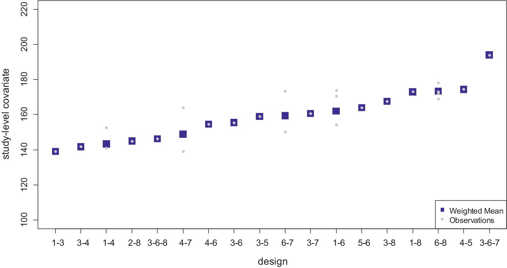
In network meta-analysis, not only consistency but also transitivity is regarded as a fundamental and essential assumption,Reference Salanti ²² as it underpins the premise that indirect comparisons are theoretically valid even in the absence of direct evidence. To date, no standard statistical method has been firmly established for evaluating transitivity. However, Cipriani, Furukawa, Salanti et al.Reference Cipriani, Furukawa and Salanti ⁵² illustrated an approach in which the distributions of key covariates are compared across designs using side-by-side boxplots, thereby enabling an assessment of heterogeneity in covariate distributions. In the NMA package, the transitivity function generates such side-by-side boxplots to facilitate the evaluation of transitivity.

> transitivity(hf2, SBP, yrange=c(100,220))

(The side-by-side boxplot created is shown in Figure 6 .)

Figure 6.

Side-by-side boxplot for assessing transitivity in the antihypertensive drug study created using the transitivity function.

Figure 6. Long description

The y-axis is labeled study-level covariate with a scale from 100 to 220 in increments of 20. The x-axis is labeled design and contains 18 categorical labels.

From left to right, the designs are: 1-3, 3-4, 1-4, 2-8, 3-6-8, 4-7, 4-6, 3-6, 3-5, 6-7, 3-7, 1-6, 5-6, 3-8, 1-8, 6-8, 4-5, and 3-6-7.

The data is represented by blue squares indicating the Weighted Mean and small grey dots indicating individual Observations. The Weighted Mean values follow a steady upward linear trend, starting at approximately 140 for design 1-3 and ending at approximately 195 for design 3-6-7.

Most designs show a single blue square with a central grey dot. However, designs 1-4, 4-7, 6-7, 1-6, and 6-8 show a vertical spread of multiple grey dots above and below the blue square, indicating a higher variance in observations for those specific study designs.

A legend in the bottom-right corner identifies the blue square as Weighted Mean and the grey dot as Observations.