1 Introduction
In most glacier and ice sheet models, ice is described as a viscous non-Newtonian (Glen Reference Glen1953) fluid whose motion is governed by 3D nonlinear Stokes equations (Jouvet & Rappaz Reference Jouvet and Rappaz2011). However, it is common practice to simplify the ice flow equations by neglecting higher-order terms in the aspect ratio
 $\unicode[STIX]{x1D716}$
, which is usually small, in order to reduce the complexity of the equations and the computational costs related to solving them. Among these simplified models, the Blatter model (Blatter Reference Blatter1995) relies on the ‘hydrostatic approximation’ to eliminate the pressure field and on truncations of the second-order terms in
 $\unicode[STIX]{x1D716}$
to eliminate the vertical component of the velocity. As a result, the Blatter model consists of a 3D nonlinear elliptic equation (Colinge & Rappaz Reference Colinge and Rappaz1999; Schoof Reference Schoof2010) for the horizontal velocity. Going one step further, the shallow ice approximation (Hutter Reference Hutter1983) (SIA) is obtained after dropping the first-order terms in
 $\unicode[STIX]{x1D716}$
in the Blatter model. With the resulting simplifications, the horizontal derivatives vanish and an analytical solution (Greve & Blatter Reference Greve and Blatter2009) can be manufactured from a vertical integration. As a result, the SIA analytical solution is computationally very inexpensive to solve. However, the SIA can be applied only to ice flow dominated by vertical shear without basal sliding. In contrast, the shallow shelf approximation (Morland Reference Morland, Veen and Oerlemans1987; MacAyeal Reference MacAyeal1989; Weis, Greve & Hutter Reference Weis, Greve and Hutter1999) (SSA) assumes no vertical variation in the velocity of the Blatter model, and describes only its horizontal distribution. Thus, the SSA most closely describes ice flow dominated by basal sliding as can be observed over ice shelves. Mathematically, the SSA consists of a 2D nonlinear elliptic equation for the horizontal velocity field. Although the SSA is substantially more expensive to solve than the SIA, it remains much cheaper than any 3D model. The SIA can be seen as a lubrication flow, while the SSA can be seen as a free film flow with some friction at the boundary.
Modelling of the ice flow of a mountain glacier, an ice shelf or an ice sheet requires a careful choice of mechanical model. The Stokes and Blatter models are suitable for all kinds of ice flows. However, these models are costly to solve, and thus cannot (currently) be used to simulate large time and spatial scales in high resolution. In contrast, the SIA, SSA and any linear combination of the two (Hindmarsh Reference Hindmarsh2004; Bueler & Brown Reference Bueler and Brown2009) apply only to specific ice flows, but can be run for multimillennial simulations of large ice fields (Ritz, Rommelaere & Dumas Reference Ritz, Rommelaere and Dumas2001). In conclusion, a compromise must always be found between mechanical accuracy and spatial resolution. Through modelling exercises such as ISMIP-HOM (Pattyn et al.
Reference Pattyn2008) or MISMIP (Schoof, Hindmarsch & Pattyn Reference Schoof, Hindmarsch and Pattyn2000), the validity of each model was assessed for a range of idealized ice flows that can be encountered on real glaciers and ice sheets. At a more theoretical level, there exist asymptotic analyses to assess the suitability of each model with respect to ice flow features like the aspect ratio
 $\unicode[STIX]{x1D716}$
or in the ratio of vertical to horizontal stress
 $\unicode[STIX]{x1D706}$
; see, e.g., Schoof & Hindmarsh (Reference Schoof and Hindmarsh2010). A few authors have attempted to estimate the mechanical accuracy of one simplified model as compared with its original one by estimating the error from the simplified solution. For instance, Lingle & Troshina (Reference Lingle and Troshina1998) used SIA solutions to evaluate the missing balance of longitudinal stresses, which would appear in a higher-order model. Recently, Ahlkrona et al. (Reference Ahlkrona, Lotstedt, Kirchner and Zwinger2016) used the residual of a mixed SIA–Stokes linearized system to split the SIA and the Stokes computational domains in an optimal way. In Jouvet & Picasso (Reference Jouvet and Picasso0000), an a posteriori mechanical error estimator was derived to evaluate the accuracy of the SSA as compared with the Blatter model. To the best of our knowledge, there exist no other mathematical results that are able to estimate the discrepancy between the solutions of two embedded ice flow models with respect to model set-up data.
This paper aims to fill this gap by deriving ‘mechanical’ error estimators between the most common shallow ice flow models. The approach involves variational techniques similar to the ones applied to derive a priori and a posteriori estimators of the numerical error (Colinge & Rappaz Reference Colinge and Rappaz1999; Rappaz & Reist Reference Rappaz and Reist2005; Jouvet & Rappaz Reference Jouvet and Rappaz2011). Since the goal of these estimators is to evaluate the suitability of one simplified model as compared with its immediate less shallow predecessor one, the most challenging task is to obtain an estimate that does not depend on that one, which is also the most expensive one to compute. Thus, we retain the term ‘a posteriori’ estimator, similar to numerical estimators; see, e.g., Quarteroni & Valli (Reference Quarteroni and Valli1994). In order to apply the techniques mentioned earlier, it is necessary to develop a variational and unified formulation for all of the ice flow models. To do this, the simplifications in the aspect ratio
 $\unicode[STIX]{x1D716}$
are applied for the variational form associated with the Stokes problem, instead of the strong form that is normally used; see, e.g., Greve & Blatter (Reference Greve and Blatter2009). As noticed in Dukowicz (Reference Dukowicz2012), in the variational formulation, the ‘hydrostatic approximation’ assumption is not needed as in the original derivation (Blatter Reference Blatter1995) since the pressure field does not appear explicitly in the functional to be minimized. (The pressure can be seen as a Lagrange multiplier for the incompressibility condition; see, e.g., Girault & Raviart (Reference Girault and Raviart1986).)
The outline of this paper is as follows. In § 2, the ice flow models, starting from the most general Stokes one, are written and the appropriate mathematical framework is set up. Then, in § 3, the ‘mechanical error estimators’ are derived in pairs (Blatter–SSA, Blatter–SIA, Stokes–Blatter) . Finally, in § 4, the capability of these estimators to assess the accuracy of one or the other model in the case of flowline ISMIP-HOM experiments is tested (Pattyn et al. Reference Pattyn2008).
2 Modelling
In this section, we first recall the most general model (Glen–Stokes), formulate its associated variational and minimization forms in appropriate functional spaces, and apply simplifications to obtain the shallow ice models in similar forms.
Let
 $V$
be a three-dimensional domain of ice, divided into the upper interface
 $\unicode[STIX]{x1D6E4}_{s}$
and the lower interface
 $\unicode[STIX]{x1D6E4}_{0}\cup \unicode[STIX]{x1D6E4}_{m}$
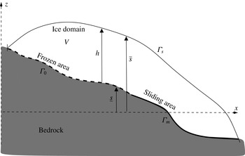
; see figure 1. At the lower interface, ice can be frozen or sliding:
 $\unicode[STIX]{x1D6E4}_{0}$
denotes the non-sliding part and
 $\unicode[STIX]{x1D6E4}_{m}$
the sliding part. We assume that
 $\unicode[STIX]{x1D6E4}_{s}$
,
 $\unicode[STIX]{x1D6E4}_{0}$
and
 $\unicode[STIX]{x1D6E4}_{m}$
are
 ${\mathcal{C}}^{1}$
.
Cross-section of an ice sheet and an ice shelf, where
 $\text{}\underline{s}$
and
 $\overline{s}$
denote the elevations of the lower and upper ice surfaces respectively,
 $h$
denotes the ice thickness, and
 $\unicode[STIX]{x1D6E4}_{s}$
denotes the upper ice surface.

2.1 Glen–Stokes model
The Stokes model consists of the momentum conservation equation when acceleration terms are ignored, together with the incompressibility condition:
 $$\begin{eqnarray}\displaystyle -\unicode[STIX]{x1D735}\boldsymbol{\cdot }\unicode[STIX]{x1D748} & = & \displaystyle \unicode[STIX]{x1D70C}\boldsymbol{g},\quad \text{in }\;V,\end{eqnarray}$$
 $$\begin{eqnarray}\displaystyle \unicode[STIX]{x1D735}\boldsymbol{\cdot }\boldsymbol{u} & = & \displaystyle 0,\quad \text{in }\;V,\end{eqnarray}$$
where
 $\unicode[STIX]{x1D748}$
is the Cauchy stress tensor,
 $\boldsymbol{g}=(0,0,-g)$
,
 $g$
is the gravitational constant and
 $\boldsymbol{u}=(u_{x},u_{y},u_{z})$
is the velocity field. Call
 $\unicode[STIX]{x1D70F}$
the deviatoric stress tensor defined by
 $$\begin{eqnarray}\unicode[STIX]{x1D748}=\unicode[STIX]{x1D70F}-PI,\end{eqnarray}$$
where
 $I$
is the identity tensor and
 $P$
is the pressure field, and by the requirement that
 $\text{tr}(\unicode[STIX]{x1D70F})=0$
so that
 $P=-(1/3)\text{tr}(\unicode[STIX]{x1D748})$
. Glen’s flow law (Glen Reference Glen1953), which describes the mechanical behaviour of ice, consists of the following nonlinear relation:
 $$\begin{eqnarray}\unicode[STIX]{x1D70F}=2\unicode[STIX]{x1D707}\unicode[STIX]{x1D63F}(\boldsymbol{u}),\end{eqnarray}$$
where
 $\unicode[STIX]{x1D63F}(\boldsymbol{u})$
denotes the strain rate tensor defined by
 $$\begin{eqnarray}\unicode[STIX]{x1D63F}(\boldsymbol{u})={\textstyle \frac{1}{2}}(\unicode[STIX]{x1D735}\boldsymbol{u}+\unicode[STIX]{x1D735}\boldsymbol{u}^{\text{T}}),\end{eqnarray}$$
 $\unicode[STIX]{x1D707}$
is the viscosity defined by
 $$\begin{eqnarray}\unicode[STIX]{x1D707}={\textstyle \frac{1}{2}}B|\unicode[STIX]{x1D63F}(\boldsymbol{u})|^{p-2},\end{eqnarray}$$
where
 $|Y|:=\sqrt{(Y:Y)}$
denotes the norm associated with the scalar product
 $(\;:\;)$
,
 $B>0$
and
 $p\in (1,2]$
are two parameters. Observe that equation (2.2) implies that
 $\unicode[STIX]{x1D63F}(\boldsymbol{u})$
has zero trace.
It is common in glaciology to express the coefficient
 $B$
and exponent
 $p$
in terms of different parameters. Define Glen’s exponent
 $n=1/(p-1)$
and then define a new rate constant
 $A=(\sqrt{2})^{n-1}B^{-n}$
. (Note that the common convention in the literature is to instead set
 $A=B^{-n}$
(e.g. Blatter Reference Blatter1995), but our convention reduces clutter in the equations.) In reality,
 $A$
and
 $B$
are not constant since they depend on the ice temperature (Glen Reference Glen1953; Paterson Reference Paterson1994), but, for the sake of simplicity, this paper assumes that the ice is isothermal.
2.2 Boundary conditions
The boundary conditions that supplement (2.1), (2.2) are the following. No force applies on the ice–air interface,
 $$\begin{eqnarray}\unicode[STIX]{x1D748}\boldsymbol{\cdot }\boldsymbol{n}=0,\quad P=0,\quad \text{on }\;\unicode[STIX]{x1D6E4}_{s},\end{eqnarray}$$
where
 $\boldsymbol{n}$
is an outer normal vector along
 $\unicode[STIX]{x1D6E4}_{s}$
. Along the lower surface interface, the no-slip condition is
 $$\begin{eqnarray}\boldsymbol{u}=\mathbf{0},\quad \text{on }\;\unicode[STIX]{x1D6E4}_{0},\end{eqnarray}$$
and the nonlinear friction condition reads (Hutter Reference Hutter1983; Schoof & Hewitt Reference Schoof and Hewitt2013)
 $$\begin{eqnarray}\displaystyle & \displaystyle \boldsymbol{u}\boldsymbol{\cdot }\boldsymbol{n}=0,\quad \text{on }\;\unicode[STIX]{x1D6E4}_{m}, & \displaystyle\end{eqnarray}$$
 $$\begin{eqnarray}\displaystyle & \displaystyle [(I-\boldsymbol{n}\boldsymbol{n}^{\text{T}})\unicode[STIX]{x1D70F}]\boldsymbol{\cdot }\boldsymbol{n}=-C|(I-\boldsymbol{n}\boldsymbol{n}^{\text{T}})\boldsymbol{\cdot }\boldsymbol{u}|^{s-2}(I-\boldsymbol{n}\boldsymbol{n}^{\text{T}})\boldsymbol{\cdot }\boldsymbol{u},\quad \text{on }\;\unicode[STIX]{x1D6E4}_{m}, & \displaystyle\end{eqnarray}$$
for
 $k\in \{x,y\}$
, where
 $s\in (1,p]$
,
 $C=C(x,y)>0$
and
 $\boldsymbol{n}$
is the outward normal unit vector to
 $\unicode[STIX]{x1D6E4}_{m}$
. Relation (2.10) relates the basal shear stress
 $[(I-\boldsymbol{n}\boldsymbol{n}^{\text{T}})\unicode[STIX]{x1D70F}]\boldsymbol{\cdot }\boldsymbol{n}$
to the sliding velocity
 $(I-\boldsymbol{n}\boldsymbol{n}^{\text{T}})\boldsymbol{\cdot }\boldsymbol{u}$
, both of them being projected onto the tangential plane.
2.3 Functional space and variational formulation
We now reformulate the Stokes problem into variational and minimization problems (Glowinski & Le Tallec Reference Glowinski and Le Tallec1989; Jouvet & Rappaz Reference Jouvet and Rappaz2011). For this, we consider the following divergence-free velocity space incorporating Dirichlet conditions where present (Girault & Raviart Reference Girault and Raviart1986):
 $$\begin{eqnarray}{\mathcal{X}}:=\{\boldsymbol{v}\in [W^{1,p}(V)]^{3},\unicode[STIX]{x1D735}\boldsymbol{\cdot }\boldsymbol{v}=0,\boldsymbol{v}=\mathbf{0}\;\text{on}\;\unicode[STIX]{x1D6E4}_{0},\boldsymbol{v}\boldsymbol{\cdot }\boldsymbol{n}=0\;\text{on}\;\unicode[STIX]{x1D6E4}_{m}\};\end{eqnarray}$$
see Adams & Fournier (Reference Adams and Fournier2003) for an introduction to the Sobolev space
 $W^{1,p}$
. In addition, we introduce several norms:
 $\Vert \cdot \Vert _{L^{p}}$
and
 $|\cdot |_{W^{1,p}}$
denote the
 $L^{p}$
norm and the
 $W^{1,p}$
seminorm, defined by
 $\Vert \boldsymbol{v}\Vert _{L^{p}}^{p}:=\int _{V}|\boldsymbol{v}|^{p}\,\text{d}V$
and
 $|\boldsymbol{v}|_{W^{1,p}}=\Vert \unicode[STIX]{x1D735}\boldsymbol{v}\Vert _{L^{p}}$
respectively. Furthermore,
 $\Vert \cdot \Vert _{W^{1,p}}$
denotes the
 $W^{1,p}$
norm defined by
 $\Vert \boldsymbol{v}\Vert _{W^{1,p}}=\Vert \boldsymbol{v}\Vert _{L^{p}}+|\boldsymbol{v}|_{W^{1,p}}$
.
From now on, we assume that
 $\unicode[STIX]{x1D6E4}_{0}$
has a non-zero measure, so that Poincaré inequality (Brezis Reference Brezis1999; Adams & Fournier Reference Adams and Fournier2003) ensures the equivalence of the norms
 $\Vert \cdot \Vert _{W^{1,p}}$
and
 $|\cdot |_{W^{1,p}}$
on the functional space
 ${\mathcal{X}}$
while Korn’s inequality (e.g. Quarteroni & Valli Reference Quarteroni and Valli1994; Ern & Guermond Reference Ern and Guermond2004) implies the equivalence of the norms
 $\Vert \cdot \Vert _{W^{1,p}}$
and the one defined by
 $\Vert \unicode[STIX]{x1D63F}(\cdot )\Vert _{L^{p}}$
on the space
 ${\mathcal{X}}$
. (One can get rid of this assumption. However, one then has to replace
 ${\mathcal{X}}$
by its quotient set induced by rigid body motions (Schoof Reference Schoof2010), otherwise Poincaré inequality is no longer valid. Doing so makes the analysis substantially more complex.) The Poincaré and Korn inequalities can be summarized by the following lemma, whose proof is found in the above references.
Lemma 1. If
 $|\unicode[STIX]{x1D6E4}_{0}|>0$
, there exist constants
 $c_{p},c_{k}>0$
such that for all
 $\boldsymbol{v}\in {\mathcal{X}}$
 $$\begin{eqnarray}\displaystyle & \Vert \boldsymbol{v}\Vert _{L^{p}}\leqslant c_{p}\Vert \unicode[STIX]{x1D735}\boldsymbol{v}\Vert _{L^{p}}, & \displaystyle\end{eqnarray}$$
 $$\begin{eqnarray}\displaystyle & \Vert \unicode[STIX]{x1D735}\boldsymbol{v}\Vert _{L^{p}}\leqslant c_{k}\Vert \unicode[STIX]{x1D63F}(\boldsymbol{v})\Vert _{L^{p}}. & \displaystyle\end{eqnarray}$$
Remark.
Constant
 $c_{p}$
in (2.12) has units of length while constant
 $c_{k}$
in (2.13) is dimensionless.
We now formulate the weak form of the Glen–Stokes model. After using (2.3), multiplying (2.1) by a test function
 $\boldsymbol{v}\in {\mathcal{X}}$
, integrating over
 $V$
, and using Gauß’s theorem twice, we obtain
 $$\begin{eqnarray}\displaystyle & & \displaystyle \int _{V}\unicode[STIX]{x1D70F}:(\unicode[STIX]{x1D735}\boldsymbol{v})\,\text{d}V-\int _{\unicode[STIX]{x2202}V}\boldsymbol{v}\boldsymbol{\cdot }(\unicode[STIX]{x1D70F}\boldsymbol{n})\,\text{d}S-\int _{V}P(\unicode[STIX]{x1D735}\boldsymbol{\cdot }\boldsymbol{v})\,\text{d}V\nonumber\\ \displaystyle & & \displaystyle \quad +\,\int _{\unicode[STIX]{x2202}V}P(\boldsymbol{v}\boldsymbol{\cdot }\boldsymbol{n})\,\text{d}S=\unicode[STIX]{x1D70C}\int _{V}\boldsymbol{g}\boldsymbol{\cdot }\boldsymbol{v}\,\text{d}V.\end{eqnarray}$$
First, by (2.4) and (2.6), the first term of (2.14) is
 $$\begin{eqnarray}\displaystyle \int _{V}\unicode[STIX]{x1D70F}:(\unicode[STIX]{x1D735}\boldsymbol{v})\,\text{d}V=\int _{V}B|\unicode[STIX]{x1D63F}(\boldsymbol{u})|^{p-2}(\unicode[STIX]{x1D63F}(\boldsymbol{u}):\unicode[STIX]{x1D63F}(\boldsymbol{v}))\,\text{d}V. & & \displaystyle\end{eqnarray}$$
Second, using (2.7a,b
), (2.8), (2.9), (2.10) and
 $\boldsymbol{v}\boldsymbol{\cdot }\boldsymbol{n}=0$
, the second term of (2.14) becomes
 $$\begin{eqnarray}\displaystyle -\int _{\unicode[STIX]{x2202}V}\boldsymbol{v}\boldsymbol{\cdot }(\unicode[STIX]{x1D70F}\boldsymbol{n})\,\text{d}S=\int _{\unicode[STIX]{x1D6E4}_{m}}C|\boldsymbol{u}|^{s-2}(\boldsymbol{u}\boldsymbol{\cdot }\boldsymbol{v})\,\text{d}S, & & \displaystyle\end{eqnarray}$$
after noting that
 $\boldsymbol{v}\boldsymbol{\cdot }\boldsymbol{n}=0$
implies
 $([(\boldsymbol{n}\boldsymbol{n}^{\text{T}})\unicode[STIX]{x1D70F}]\boldsymbol{\cdot }\boldsymbol{n})\boldsymbol{\cdot }\boldsymbol{v}=0$
and
 $[(\boldsymbol{n}\boldsymbol{n}^{\text{T}})\boldsymbol{\cdot }\boldsymbol{u}]\boldsymbol{\cdot }\boldsymbol{v}=0$
. Finally, since
 $\boldsymbol{v}$
satisfies the constraints of the functional space
 ${\mathcal{X}}$
(see (2.11)), the third and fourth terms of (2.14) are cancelled out such that the pressure field
 $P$
vanishes from the variational formulation, which simplifies to
 $$\begin{eqnarray}\displaystyle \int _{V}B|\unicode[STIX]{x1D63F}(\boldsymbol{u})|^{p-2}(\unicode[STIX]{x1D63F}(\boldsymbol{u}):\unicode[STIX]{x1D63F}(\boldsymbol{v}))\,\text{d}V+\int _{\unicode[STIX]{x1D6E4}_{m}}C|\boldsymbol{u}|^{s-2}(\boldsymbol{u}\boldsymbol{\cdot }\boldsymbol{v})\,\text{d}S=\unicode[STIX]{x1D70C}\int _{V}\boldsymbol{g}\boldsymbol{\cdot }\boldsymbol{v}\,\text{d}V. & & \displaystyle\end{eqnarray}$$
The above variational formulation (without pressure) is usually called the ‘reduced’ formulation. In contrast, there exists a ‘mixed’ formulation, in which the pressure
 $P$
plays the role of a Lagrange multilayer for the constraint
 $\unicode[STIX]{x1D735}\boldsymbol{\cdot }\boldsymbol{u}=0$
; see, e.g., Girault & Raviart (Reference Girault and Raviart1986). In this paper, we work only with the ‘reduced’ formulation.
2.4 Minimization formulation and well-posedness
The problem defined by (2.17) can be associated with the following minimization problem (Jouvet & Rappaz Reference Jouvet and Rappaz2011):
 $$\begin{eqnarray}\displaystyle {\mathcal{J}}(\boldsymbol{u})=\text{min}\{{\mathcal{J}}(\boldsymbol{v}),\boldsymbol{v}\in {\mathcal{X}}\}, & & \displaystyle\end{eqnarray}$$
where
 $$\begin{eqnarray}\displaystyle {\mathcal{J}}(\boldsymbol{v})=\int _{V}\frac{B}{p}|\unicode[STIX]{x1D63F}(\boldsymbol{v})|^{p}\,\text{d}V+\int _{\unicode[STIX]{x1D6E4}_{m}}\frac{C}{s}|\boldsymbol{v}|^{s}\,\text{d}S-\unicode[STIX]{x1D70C}\int _{V}(\boldsymbol{g}\boldsymbol{\cdot }\boldsymbol{v})\,\text{d}V. & & \displaystyle\end{eqnarray}$$
Indeed, it is easy to verify that (2.17) corresponds to
 $\langle {\mathcal{J}}^{\prime }(\boldsymbol{u}),\boldsymbol{v}\rangle =0$
, where
 $\langle {\mathcal{J}}^{\prime }(\boldsymbol{u}),\boldsymbol{v}\rangle$
is the Gâteaux derivative of
 ${\mathcal{J}}$
at
 $\boldsymbol{u}$
in the direction
 $\boldsymbol{v}$
. One can prove the strong continuity and the convexity of
 ${\mathcal{J}}$
in
 ${\mathcal{X}}$
directly from (2.19); see lemma 2.4 and lemma 2.5 in Jouvet & Rappaz (Reference Jouvet and Rappaz2011). On the other hand, one needs the Poincaré and Korn inequalities (2.12)–(2.13) in order to prove the strict convexity of
 ${\mathcal{J}}$
and the coercivity property,
 $$\begin{eqnarray}{\mathcal{J}}(\boldsymbol{v})\geqslant c_{1}|\boldsymbol{v}|_{W^{1,p}}^{p}-c_{2},\end{eqnarray}$$
where
 $c_{1},c_{2}$
are positive constants; see lemma 2.5 and lemma 2.6 in Jouvet & Rappaz (Reference Jouvet and Rappaz2011). Following arguments of convex analysis (Girault & Raviart Reference Girault and Raviart1986), this implies the existence and the uniqueness of a minimizer of
 ${\mathcal{J}}$
in
 ${\mathcal{X}}$
(Jouvet & Rappaz Reference Jouvet and Rappaz2011), and, equivalently, the well-posedness of the variational problem (2.17). Let us note that one can show the existence of a unique pressure field
 $P$
such that
 $(\boldsymbol{u},P)$
satisfies the ‘mixed’ formulation associated with (2.17), supposing an inf–sup condition for the functional spaces of velocity and pressure; see Jouvet & Rappaz (Reference Jouvet and Rappaz2011).
2.5 Partial elimination of the vertical velocity
We could continue working with the reduced weak formulation (2.17). However, it is advantageous to eliminate the vertical component of the velocity,
 $u_{z}$
, from the formulation whenever this is possible. A closer look at (2.17) shows that this is already possible for the two last terms.
From now on, we assume that
 $$\begin{eqnarray}\left.\begin{array}{@{}l@{}}\displaystyle V=\{(x,y,z),\text{}\underline{s}(x,y)\leqslant z\leqslant \overline{s}(x,y)\},\\ \displaystyle \unicode[STIX]{x1D6E4}_{s}=\{(x,y,z),z=\overline{s}(x,y)\},\\ \displaystyle \unicode[STIX]{x1D6E4}_{0}\cup \unicode[STIX]{x1D6E4}_{m}=\{(x,y,z),z=\text{}\underline{s}(x,y)\},\end{array}\right\}\end{eqnarray}$$
where
 $\boldsymbol{x}=(x,y)$
denotes the horizontal coordinates,
 $z$
denotes the vertical coordinate, and
 $\text{}\underline{s}(x,y)$
and
 $\overline{s}(x,y)$
are the elevations of the lower and upper ice surfaces; see figure 1. The ice thickness is denoted by
 $h$
and satisfies
 $h=\overline{s}-\text{}\underline{s}$
.
In fact,
 $\boldsymbol{u}\boldsymbol{\cdot }\boldsymbol{n}=0$
and
 $\boldsymbol{v}\boldsymbol{\cdot }\boldsymbol{n}=0$
on
 $\unicode[STIX]{x1D6E4}_{m}$
imply
 $$\begin{eqnarray}\displaystyle \boldsymbol{u}\boldsymbol{\cdot }\boldsymbol{v}=\left(\begin{array}{@{}c@{}}u_{x}\\ u_{y}\end{array}\right)\boldsymbol{\cdot }\left(\begin{array}{@{}c@{}}v_{x}\\ v_{y}\end{array}\right)+\left[\unicode[STIX]{x1D735}_{\boldsymbol{x}}\text{}\underline{s}\cdot \left(\begin{array}{@{}c@{}}u_{x}\\ u_{y}\end{array}\right)\right]\times \left[\unicode[STIX]{x1D735}_{\boldsymbol{x}}\text{}\underline{s}\cdot \left(\begin{array}{@{}c@{}}v_{x}\\ v_{y}\end{array}\right)\right], & & \displaystyle\end{eqnarray}$$
where
 $\unicode[STIX]{x1D735}_{\boldsymbol{x}}$
is the gradient with respect to the horizontal coordinates
 $\boldsymbol{x}=(x,y)$
and
 $\boldsymbol{n}^{\text{T}}=((\unicode[STIX]{x1D735}_{\boldsymbol{x}}\text{}\underline{s})^{\text{T}},-1)$
. This defines a scalar product
 $(\boldsymbol{a},\boldsymbol{b})_{M}:=(\unicode[STIX]{x1D648}\boldsymbol{a})\boldsymbol{\cdot }\boldsymbol{b}$
and its associated norm
 $|\boldsymbol{a}|_{M}:=\sqrt{(\boldsymbol{a},\boldsymbol{ a})_{M}}$
, where the
 $3\times 3$
matrix
 $\unicode[STIX]{x1D648}$
is defined by
 $$\begin{eqnarray}\displaystyle \unicode[STIX]{x1D648}=\left(\begin{array}{@{}cc@{}}I+(\unicode[STIX]{x1D735}_{\boldsymbol{x}}\text{}\underline{s})(\unicode[STIX]{x1D735}_{\boldsymbol{x}}\text{}\underline{s})^{\text{T}} & \mathbf{0}\\ \mathbf{0} & 0\end{array}\right), & & \displaystyle\end{eqnarray}$$
so that
 $$\begin{eqnarray}\displaystyle \int _{\unicode[STIX]{x1D6E4}_{m}}C|\boldsymbol{u}|^{s-2}(\boldsymbol{u}\boldsymbol{\cdot }\boldsymbol{v})\,\text{d}S=\int _{\unicode[STIX]{x1D6E4}_{m}}C|\boldsymbol{u}|_{M}^{s-2}(\boldsymbol{u},\boldsymbol{v})_{M}\,\text{d}S. & & \displaystyle\end{eqnarray}$$
Since the last row of
 $\unicode[STIX]{x1D648}$
in (2.23) is filled with zeroes, (2.24) shows that the second term in (2.17) does not actually depend on the last component
 $u_{z}$
.
On the other hand, using the Gauß theorem we have, for any
 $\boldsymbol{v}\in {\mathcal{X}}$
(see (2.11)),
 $$\begin{eqnarray}\displaystyle \int _{V}(\unicode[STIX]{x1D735}\overline{s}\boldsymbol{\cdot }\boldsymbol{v}-v_{z})\,\text{d}V & = & \displaystyle \int _{V}\boldsymbol{v}\boldsymbol{\cdot }\unicode[STIX]{x1D735}(\overline{s}-z)=-\int _{V}(\unicode[STIX]{x1D735}\boldsymbol{\cdot }\boldsymbol{v})(\overline{s}-z)\,\text{d}V\nonumber\\ \displaystyle & & \displaystyle +\,\int _{\unicode[STIX]{x2202}V}(\overline{s}-z)(\boldsymbol{v}\boldsymbol{\cdot }\boldsymbol{n})\,\text{d}S=0.\end{eqnarray}$$
As a consequence, the right-hand side in (2.17) can be formulated without the vertical component of the velocity:
 $$\begin{eqnarray}\displaystyle \unicode[STIX]{x1D70C}\int _{V}\boldsymbol{g}\boldsymbol{\cdot }\boldsymbol{v}\,\text{d}V=-\unicode[STIX]{x1D70C}g\int _{V}(\unicode[STIX]{x1D735}\overline{s}\boldsymbol{\cdot }\boldsymbol{v})\,\text{d}V. & & \displaystyle\end{eqnarray}$$
In summary, the variational formulation (2.17) can now be rewritten as
 $$\begin{eqnarray}\displaystyle & & \displaystyle \int _{V}B|\unicode[STIX]{x1D63F}(\boldsymbol{u})|^{p-2}(\unicode[STIX]{x1D63F}(\boldsymbol{u}),\unicode[STIX]{x1D63F}(\boldsymbol{v}))\,\text{d}V+\int _{\unicode[STIX]{x1D6E4}_{m}}C|\boldsymbol{u}|_{M}^{s-2}(\boldsymbol{u},\boldsymbol{v})_{M}\text{d}S+\unicode[STIX]{x1D70C}g\int _{V}(\unicode[STIX]{x1D735}\overline{s}\boldsymbol{\cdot }\boldsymbol{v})\,\text{d}V=0,\nonumber\\ \displaystyle & & \displaystyle\end{eqnarray}$$
while the functional to be minimized is
 $$\begin{eqnarray}\displaystyle {\mathcal{J}}(\boldsymbol{v})=\int _{V}\frac{B}{p}|\unicode[STIX]{x1D63F}(\boldsymbol{v})|^{p}\,\text{d}V+\int _{\unicode[STIX]{x1D6E4}_{m}}\frac{C}{s}|\boldsymbol{v}|_{M}^{s}\,\text{d}S+\unicode[STIX]{x1D70C}g\int _{V}(\unicode[STIX]{x1D735}\overline{s}\boldsymbol{\cdot }\boldsymbol{v})\,\text{d}V. & & \displaystyle\end{eqnarray}$$
It must be stressed that only the first term still depends on the vertical velocity in both formulations (2.27) and (2.28).
2.6 Shallow ice flow models
In this section, we infer the classical shallow ice flow models (Blatter, SIA and SSA) by applying simplifications to the Glen–Stokes model at the variational level.
Let us define
 $\unicode[STIX]{x1D63F}_{0}(\boldsymbol{u})$
,
 $\unicode[STIX]{x1D63F}_{1}(\boldsymbol{u})$
and
 $\unicode[STIX]{x1D63F}_{2}(\boldsymbol{u})$
by splitting the strain rate tensor as follows:
 $$\begin{eqnarray}\displaystyle \unicode[STIX]{x1D63F}(\boldsymbol{u})=\unicode[STIX]{x1D63F}_{0}(\boldsymbol{u})+\unicode[STIX]{x1D63F}_{1}(\boldsymbol{u})+\unicode[STIX]{x1D63F}_{2}(\boldsymbol{u}), & & \displaystyle\end{eqnarray}$$
where
 $$\begin{eqnarray}\displaystyle \unicode[STIX]{x1D63F}_{0}(\boldsymbol{u}) & = & \displaystyle \left(\begin{array}{@{}ccc@{}}0 & 0 & \displaystyle {\textstyle \frac{1}{2}}(\unicode[STIX]{x2202}_{z}u_{x})\\ 0 & 0 & \displaystyle {\textstyle \frac{1}{2}}(\unicode[STIX]{x2202}_{z}u_{y})\\ \displaystyle {\textstyle \frac{1}{2}}(\unicode[STIX]{x2202}_{z}u_{x}) & \displaystyle {\textstyle \frac{1}{2}}(\unicode[STIX]{x2202}_{z}u_{y}) & 0\end{array}\right),\end{eqnarray}$$
 $$\begin{eqnarray}\displaystyle \unicode[STIX]{x1D63F}_{1}(\boldsymbol{u}) & = & \displaystyle \displaystyle \left(\begin{array}{@{}ccc@{}}\unicode[STIX]{x2202}_{x}u_{x} & \displaystyle {\textstyle \frac{1}{2}}(\unicode[STIX]{x2202}_{y}u_{x}+\unicode[STIX]{x2202}_{x}u_{y}), & 0\\ \displaystyle {\textstyle \frac{1}{2}}(\unicode[STIX]{x2202}_{y}u_{x}+\unicode[STIX]{x2202}_{x}u_{y}) & \unicode[STIX]{x2202}_{y}u_{y} & 0\\ 0 & 0 & -\unicode[STIX]{x2202}_{x}u_{x}-\unicode[STIX]{x2202}_{y}u_{y}\end{array}\right),\end{eqnarray}$$
 $$\begin{eqnarray}\displaystyle \unicode[STIX]{x1D63F}_{2}(\boldsymbol{u}) & = & \displaystyle \left(\begin{array}{@{}ccc@{}}0 & 0 & \displaystyle {\textstyle \frac{1}{2}}(\unicode[STIX]{x2202}_{x}u_{z})\\ 0 & 0 & \displaystyle {\textstyle \frac{1}{2}}(\unicode[STIX]{x2202}_{y}u_{z})\\ \displaystyle {\textstyle \frac{1}{2}}(\unicode[STIX]{x2202}_{x}u_{z}) & \displaystyle {\textstyle \frac{1}{2}}(\unicode[STIX]{x2202}_{y}u_{z}) & 0\end{array}\right),\end{eqnarray}$$
where
 $\unicode[STIX]{x1D63F}_{0}$
and
 $\unicode[STIX]{x1D63F}_{1}$
depend only on the horizontal velocity components
 $(u_{x},u_{y})$
while
 $\unicode[STIX]{x1D63F}_{2}$
depends on the horizontal derivatives of the vertical component. We also define
 $\unicode[STIX]{x1D63F}_{01}(\boldsymbol{u}):=\unicode[STIX]{x1D63F}_{0}(\boldsymbol{u})+\unicode[STIX]{x1D63F}_{1}(\boldsymbol{u})$
, and
 $\unicode[STIX]{x1D63F}_{02}(\boldsymbol{u}):=\unicode[STIX]{x1D63F}_{0}(\boldsymbol{u})+\unicode[STIX]{x1D63F}_{2}(\boldsymbol{u})$
.
A hierarchy of ice sheet models is associated with an expansion in the small parameter
 $\unicode[STIX]{x1D716}=[h]/[\boldsymbol{x}]$
, the aspect ratio of the ice geometry
 $V$
. Here,
 $[h]$
and
 $[\boldsymbol{x}]$
denote its typical height and length. It is easy to verify that in the splitting (2.29),
 $\unicode[STIX]{x1D63F}_{0}$
scales with
 $1/\unicode[STIX]{x1D716}$
,
 $\unicode[STIX]{x1D63F}_{1}$
scales with
 $1$
(i.e. it is dimensionless) and
 $\unicode[STIX]{x1D63F}_{2}$
scales with
 $\unicode[STIX]{x1D716}$
. From this observation, one can obtain submodels by neglecting the second-order component
 $\unicode[STIX]{x1D63F}_{2}$
or/and the first-order component
 $\unicode[STIX]{x1D63F}_{1}$
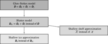
in (2.29). Figure 2, and the paragraphs below, describe this hierarchy by identifying replacements for the full tensor
 $\unicode[STIX]{x1D63F}(\boldsymbol{u})$
. Looking forward, the estimators in § 3 are in one-to-one correspondence with the arrows in figure 2.
The hierarchy of the ice flow models.

The Blatter model (Blatter Reference Blatter1995) is obtained by neglecting
 $\unicode[STIX]{x1D63F}_{2}(\boldsymbol{u})$
, or equivalently by replacing
 $\unicode[STIX]{x1D63F}(\boldsymbol{u})$
by
 $\unicode[STIX]{x1D63F}_{01}(\boldsymbol{u})$
in the formulation (2.27) or (2.28). As a consequence, the variational formulation is
 $$\begin{eqnarray}\displaystyle & & \displaystyle \text{Find }\;\boldsymbol{u}_{1}\in {\mathcal{X}}\;\text{s.t. }\quad \int _{V}B|\unicode[STIX]{x1D63F}_{01}(\boldsymbol{u}_{1})|^{p-2}(\unicode[STIX]{x1D63F}_{01}(\boldsymbol{u}_{1}):\unicode[STIX]{x1D63F}_{01}(\boldsymbol{v}))\,\text{d}V\nonumber\\ \displaystyle & & \displaystyle \quad +\,\int _{\unicode[STIX]{x1D6E4}_{m}}C|\boldsymbol{u}_{1}|_{M}^{s-2}(\boldsymbol{u}_{1},\boldsymbol{v})_{M}\text{d}S+\unicode[STIX]{x1D70C}g\int _{V}(\unicode[STIX]{x1D735}\overline{s}\boldsymbol{\cdot }\boldsymbol{v})\,\text{d}V=0,\quad \forall \boldsymbol{v}\in {\mathcal{X}},\end{eqnarray}$$
where
 $\boldsymbol{u}_{1}$
denotes the Blatter solution. By doing so, the variational equality no longer involves any vertical component of the velocity. As a consequence, the Blatter model solves the horizontal components of the velocity only, and
 $u_{z}$
can be computed a posteriori from the horizontal components by integrating the incompressibility condition,
 $$\begin{eqnarray}\displaystyle \unicode[STIX]{x2202}_{k}u_{z}=-\unicode[STIX]{x2202}_{k}\left(\int _{b}^{z}(\unicode[STIX]{x2202}_{x}u_{x}+\unicode[STIX]{x2202}_{y}u_{y})\,\text{d}z\right), & & \displaystyle\end{eqnarray}$$
for
 $k\in \{x,y\}$
.
In solving (2.33), one can remove the third component from the definition of the functional space
 ${\mathcal{X}}$
together with the incompressibility condition. Let
 $\hat{{\mathcal{X}}}$
be the space
 ${\mathcal{X}}$
but with the vertical velocity component removed. One can then show that any solution
 $\boldsymbol{u}_{1}\in {\mathcal{X}}$
of (2.33) minimizes (2.28), with
 $\unicode[STIX]{x1D63F}$
being replaced by
 $\unicode[STIX]{x1D63F}_{01}$
, and vice versa with the solution of (2.33) from
 $\hat{{\mathcal{X}}}$
being extended by solving (2.34). (For simplicity, we keep the notation
 ${\mathcal{X}}$
to denote
 $\hat{{\mathcal{X}}}$
in what follows.) In addition, the functional conserves all of its properties such that the existence and uniqueness of a minimizer are automatically ensured; see Colinge & Rappaz (Reference Colinge and Rappaz1999) and Schoof (Reference Schoof2010). The traditional Blatter model derivation involves the ‘hydrostatic approximation’ assumption. It is used to get rid of the pressure and to transfer the gravitational forces on the right-hand side of the momentum conservation equations from the vertical to the horizontal components. In the current approach, the ‘hydrostatic approximation’ assumption is not needed since the pressure
 $P$
is eliminated by restricting the functional space for the velocity field to divergence-free fields (§ 2.3), while this transfer of the gravitational force components results from the application of the Gauß theorem (§ 2.5), as already mentioned in Dukowicz (Reference Dukowicz2012). Thus, working with the weak form of the Stokes equation instead of the strong original form makes the derivation simpler. Although one can rewrite (2.33) in a simplified subspace of
 ${\mathcal{X}}$
, we deliberately keep the formulation intact in order to obtain a unified formulation for all submodels.
Going one step further, the SIA (Hutter Reference Hutter1983) is obtained by neglecting
 $\unicode[STIX]{x1D63F}_{1}$
, or equivalently by replacing
 $\unicode[STIX]{x1D63F}_{01}$
by
 $\unicode[STIX]{x1D63F}_{0}$
in (2.33). As a consequence, the variational formulation for the SIA is
 $$\begin{eqnarray}\displaystyle & & \displaystyle \text{find }\;\boldsymbol{u}_{0}\in {\mathcal{X}}\;\text{s.t. }\quad \int _{V}B|\unicode[STIX]{x1D63F}_{0}(\boldsymbol{u}_{0})|^{p-2}(\unicode[STIX]{x1D63F}_{0}(\boldsymbol{u}_{0}):\unicode[STIX]{x1D63F}_{0}(\boldsymbol{v}))\,\text{d}V\nonumber\\ \displaystyle & & \displaystyle \quad +\,\int _{\unicode[STIX]{x1D6E4}_{m}}C|\boldsymbol{u}_{0}|_{M}^{s-2}(\boldsymbol{u}_{0},\boldsymbol{v})_{M}\text{d}S+\unicode[STIX]{x1D70C}g\int _{V}(\unicode[STIX]{x1D735}\overline{s}\boldsymbol{\cdot }\boldsymbol{v})\,\text{d}V=0,\quad \forall \boldsymbol{v}\in {\mathcal{X}},\end{eqnarray}$$
where
 $\boldsymbol{u}_{0}$
denotes the SIA solution. As in the Blatter model, (2.35) does not involve
 $u_{z}$
. Furthermore, the first term in (2.35) now contains only vertical derivatives, but no more horizontal derivatives. The removal of these horizontal derivatives renders the overall problem substantially easier to solve. In particular, the SIA solution can be written analytically, as independent vertical integrals for the horizontal components of velocity; see, e.g., Greve & Blatter (Reference Greve and Blatter2009). Because of the loss of the
 $\unicode[STIX]{x1D63F}_{1}$
term in the variational inequality, one cannot state the existence and the uniqueness of a solution as before, since Korn’s inequality no longer holds with
 $\unicode[STIX]{x1D63F}_{0}$
instead of
 $\unicode[STIX]{x1D63F}$
. However, since the associated functional contains no horizontal derivatives, one can permute ‘
 $\text{min}$
’ and horizontal integration, and then solve the problem pointwise in
 $\boldsymbol{x}$
. Call
 $\unicode[STIX]{x1D6FA}$
and
 $\unicode[STIX]{x1D6FA}_{k}$
the projections of
 $V$
and its boundaries
 $\unicode[STIX]{x1D6E4}_{k}$
on the horizontal plane
 $(Oxy)$
for
 $k\in \{s,0,m\}$
. Given
 $\boldsymbol{x}\in \unicode[STIX]{x1D6FA}$
, the pointwise minimization problem
 $$\begin{eqnarray}\displaystyle \text{min}\left\{\int _{\text{}\underline{s}(\boldsymbol{x})}^{\overline{s}(\boldsymbol{x})}\left(\frac{B}{p}|\unicode[STIX]{x1D63F}_{0}(\boldsymbol{v})|^{p}\,\text{d}z+\unicode[STIX]{x1D70C}g(\unicode[STIX]{x1D735}\overline{s}\boldsymbol{\cdot }\boldsymbol{v})\right)\,\text{d}z+\frac{C}{s}|\boldsymbol{v}(\boldsymbol{x},\text{}\underline{s}(\boldsymbol{x}))|_{M}^{s}\mathbf{1}_{\unicode[STIX]{x1D6FA}_{m}}(\boldsymbol{x})\right\} & & \displaystyle\end{eqnarray}$$
over the set of functions
 $$\begin{eqnarray}\displaystyle \left\{\boldsymbol{v}(\boldsymbol{x},\boldsymbol{\cdot })\in W^{1,p}(\text{}\underline{s}(\boldsymbol{x}),\overline{s}(\boldsymbol{x})),\text{s.t.}~\boldsymbol{v}(\boldsymbol{x},\text{}\underline{s}(\boldsymbol{x}))=0\;\text{if}\;\boldsymbol{x}\in \unicode[STIX]{x1D6FA}_{0}\right\} & & \displaystyle\end{eqnarray}$$
admits a unique solution since the functional in (2.36) is continuous, strictly convex and coercive in the functional space (2.37); see Schoof (Reference Schoof2010).
Finally, the SSA (Morland Reference Morland, Veen and Oerlemans1987) is obtained from the Blatter model by replacing the space of solutions
 ${\mathcal{X}}$
by its subspace of vertically constant horizontal component functions
 $$\begin{eqnarray}\displaystyle \overline{{\mathcal{X}}}=\{\boldsymbol{v}=(v_{x},v_{y},v_{z})\in {\mathcal{X}},\;\unicode[STIX]{x2202}_{z}v_{x}=0\;\;\text{a.e.},\;\unicode[STIX]{x2202}_{z}v_{y}=0\;\;\text{a.e.}\}\subset {\mathcal{X}}. & & \displaystyle\end{eqnarray}$$
As a consequence, the variational formulation for the SSA is
 $$\begin{eqnarray}\displaystyle & & \displaystyle \text{Find }\;\overline{\boldsymbol{u}}_{1}\in \overline{{\mathcal{X}}}\;\text{s.t. }\quad \int _{V}B|\unicode[STIX]{x1D63F}_{01}(\overline{\boldsymbol{u}}_{1})|^{p-2}(\unicode[STIX]{x1D63F}_{01}(\overline{\boldsymbol{u}}_{1}):\unicode[STIX]{x1D63F}_{01}(\boldsymbol{v}))\,\text{d}V\nonumber\\ \displaystyle & & \displaystyle \quad +\,\int _{\unicode[STIX]{x1D6E4}_{m}}C|\overline{\boldsymbol{u}}_{1}|_{M}^{s-2}(\overline{\boldsymbol{u}}_{1},\boldsymbol{v})_{M}\,\text{d}S+\unicode[STIX]{x1D70C}g\int _{V}(\unicode[STIX]{x1D735}\overline{s}\boldsymbol{\cdot }\boldsymbol{v})\,\text{d}V=0,\quad \forall \boldsymbol{v}\in \overline{{\mathcal{X}}},\end{eqnarray}$$
where
 $\overline{\boldsymbol{u}}_{1}$
denotes the SSA solution. Again, (2.39) does not involve
 $u_{z}$
. Note that, if
 $\boldsymbol{v}\in \overline{{\mathcal{X}}}$
, then
 $\unicode[STIX]{x1D63F}_{01}(\boldsymbol{v})$
simplifies into
 $\unicode[STIX]{x1D63F}_{1}(\boldsymbol{v})$
in (2.39). However, we keep this form intact in the following. Since the space
 $\overline{{\mathcal{X}}}$
is a closed and convex subset of
 ${\mathcal{X}}$
,
 ${\mathcal{J}}$
admits a unique minimum in
 $\overline{{\mathcal{X}}}$
,
 $\overline{\boldsymbol{u}}_{1}$
the unique solution of (2.39); see also Schoof (Reference Schoof2006).
2.7 Stability with respect to data
The next lemma shows that all of the solutions are bounded by functions of the model data.
Lemma 2. The Stokes, Blatter, SIA or SSA solutions satisfy
 $$\begin{eqnarray}|\boldsymbol{v}|_{W^{1,p}}\leqslant \left(\frac{c_{k}^{p}c_{p}\unicode[STIX]{x1D70C}g}{B}\Vert \unicode[STIX]{x1D735}\overline{s}\Vert _{L^{q}}\right)^{1/p-1},\quad \forall \boldsymbol{v}\in \{\boldsymbol{u},\boldsymbol{u}_{1},\overline{\boldsymbol{u}}_{1},\boldsymbol{u}_{0}\},\end{eqnarray}$$
where
 $q$
is defined by
 $1/p+1/q=1$
.
Proof. Let us first show (2.40) for Stokes (i.e.
 $Z=T$
) following (Jouvet Reference Jouvet2010). Setting
 $\boldsymbol{v}=\boldsymbol{u}$
in (2.27), using the Korn and Poincaré inequalities, we obtain
 $$\begin{eqnarray}\displaystyle |\boldsymbol{u}|_{W^{1,p}}^{p} & {\leqslant} & \displaystyle \frac{c_{k}^{p}}{B}\left(\int _{V}B|\unicode[STIX]{x1D63F}(\boldsymbol{u})|^{p}\,\text{d}V+\int _{\unicode[STIX]{x1D6E4}_{m}}C|\boldsymbol{u}|_{M}^{s}\,\text{d}S\right)=\frac{c_{k}^{p}\unicode[STIX]{x1D70C}g}{B}\int _{V}(\unicode[STIX]{x1D735}\overline{s}\boldsymbol{\cdot }\boldsymbol{u})\,\text{d}V\nonumber\\ \displaystyle & {\leqslant} & \displaystyle \frac{c_{k}^{p}\unicode[STIX]{x1D70C}g}{B}\Vert \unicode[STIX]{x1D735}\overline{s}\Vert _{L^{q}}\Vert \boldsymbol{u}\Vert _{L^{p}}\leqslant \frac{c_{p}c_{k}^{p}\unicode[STIX]{x1D70C}g}{B}\Vert \unicode[STIX]{x1D735}\overline{s}\Vert _{L^{q}}|\boldsymbol{u}|_{W^{1,p}},\end{eqnarray}$$
which is (2.40). It is straightforward to apply the same technique for the Blatter model (
 $\boldsymbol{u}_{1}$
) and the SSA (
 $\overline{\boldsymbol{u}}_{1}$
), but not for the SIA (
 $\boldsymbol{u}_{0}$
) since Korn’s inequality no longer holds. However, one can work pointwise by fixing
 $\boldsymbol{x}$
and integrating vertically from
 $\text{}\underline{s}(\boldsymbol{x})$
to
 $\overline{s}(\boldsymbol{x})$
instead of
 $V$
:
 $$\begin{eqnarray}|\boldsymbol{u}_{0}(\boldsymbol{x},\boldsymbol{\cdot })|_{W^{1,p}(\text{}\underline{s}(\boldsymbol{x}),\overline{s}(\boldsymbol{x}))}^{p}\leqslant \left(\frac{c_{k}^{p}c_{p}\unicode[STIX]{x1D70C}g}{B}\right)^{p/p-1}\Vert \unicode[STIX]{x1D735}\overline{s}\Vert _{L^{q}(\text{}\underline{s}(\boldsymbol{x}),\overline{s}(\boldsymbol{x}))}^{q}.\end{eqnarray}$$
It remains to integrate on the horizontal plane
 $(Oxy)$
and to take the
 $1/p$
root to obtain (2.40) for
 $\boldsymbol{v}=\boldsymbol{u}_{0}$
.
3 Derivation of estimators
The goal of this section is to prove the following theorem, which is the main object of this paper.
Theorem 1. Let
 $\boldsymbol{u}$
be the Stokes solution of (2.27),
 $\boldsymbol{u}_{1}$
be the Blatter solution of (2.33),
 $\boldsymbol{u}_{0}$
be the SIA solution of (2.35) and
 $\overline{\boldsymbol{u}}_{1}$
be the SSA solution of (2.39).
-
(1) The following estimate between the SSA and Blatter solutions holds:
(3.1)where $$\begin{eqnarray}\displaystyle \frac{|\boldsymbol{u}_{1}-\overline{\boldsymbol{u}}_{1}|_{W^{1,p}}}{|\overline{\boldsymbol{u}}_{1}|_{W^{1,p}}}\leqslant \frac{c}{B}\left[\frac{c_{k}^{p}c_{p}\unicode[STIX]{x1D70C}g}{B}\Vert \unicode[STIX]{x1D735}\overline{s}\Vert _{L^{q}}\right]^{2-p/p-1}\frac{(\unicode[STIX]{x1D702}_{1}+\unicode[STIX]{x1D702}_{2}+\unicode[STIX]{x1D702}_{3})}{|\overline{\boldsymbol{u}}_{1}|_{W^{1,p}}}, & & \displaystyle\end{eqnarray}$$
(3.2)
$$\begin{eqnarray}\displaystyle \left.\begin{array}{@{}c@{}}\displaystyle \unicode[STIX]{x1D702}_{1}=\Vert h\times (-B\unicode[STIX]{x1D735}\boldsymbol{\cdot }(|\unicode[STIX]{x1D63F}_{1}(\overline{\boldsymbol{u}}_{1})|^{p-2}\unicode[STIX]{x1D63F}_{1}(\overline{\boldsymbol{u}}_{1}))+\unicode[STIX]{x1D70C}g\unicode[STIX]{x1D735}\overline{s})\Vert _{L^{q}(V)},\\ \displaystyle \unicode[STIX]{x1D702}_{2}=\Vert h^{1/q}\times (B[|\unicode[STIX]{x1D63F}_{1}(\overline{\boldsymbol{u}}_{1})|^{p-2}\unicode[STIX]{x1D63F}_{1}(\overline{\boldsymbol{u}}_{1})]\boldsymbol{\cdot }\boldsymbol{n}+C|\overline{\boldsymbol{u}}_{1}|_{M}^{s-2}(M\overline{\boldsymbol{u}}_{1}))\Vert _{L^{q}(\unicode[STIX]{x1D6E4}_{m})},\\ \displaystyle \unicode[STIX]{x1D702}_{3}=\Vert h^{1/q}\times (B[|\unicode[STIX]{x1D63F}_{1}(\overline{\boldsymbol{u}}_{1})|^{p-2}\unicode[STIX]{x1D63F}_{1}(\overline{\boldsymbol{u}}_{1})]\boldsymbol{\cdot }\boldsymbol{n})\Vert _{L^{q}(\unicode[STIX]{x1D6E4}_{s})}.\end{array}\right\} & & \displaystyle\end{eqnarray}$$
-
(2) The following estimate between the Blatter and SIA solutions holds:
(3.3)
$$\begin{eqnarray}\displaystyle \frac{|\boldsymbol{u}_{1}-\boldsymbol{u}_{0}|_{W^{1,p}}}{|\boldsymbol{u}_{0}|_{W^{1,p}}}\leqslant c\left[\frac{c_{k}^{p}c_{p}\unicode[STIX]{x1D70C}g}{B}\Vert \unicode[STIX]{x1D735}\overline{s}\Vert _{L^{q}}\right]^{2-p/p-1}\frac{\Vert |\unicode[STIX]{x1D63F}_{01}(\boldsymbol{u}_{0})|^{p-2}|\unicode[STIX]{x1D63F}_{1}(\boldsymbol{u}_{0})|\Vert _{L^{q}}}{|\boldsymbol{u}_{0}|_{W^{1,p}}}. & & \displaystyle\end{eqnarray}$$
-
(3) In addition, if we assume no basal sliding (i.e.
$\unicode[STIX]{x1D6E4}_{m}=\emptyset$
), then the following estimate between the Stokes and Blatter solutions holds: (3.4)Here,
$$\begin{eqnarray}\displaystyle & & \displaystyle \frac{|\boldsymbol{u}_{1}-\boldsymbol{u}|_{W^{1,p}}}{|\boldsymbol{u}_{1}|_{W^{1,p}}}\leqslant c\left[\frac{c_{k}^{p}c_{p}\unicode[STIX]{x1D70C}g}{B}\Vert \unicode[STIX]{x1D735}\overline{s}\Vert _{L^{q}}\right]^{2-p/p-1}\nonumber\\ \displaystyle & & \displaystyle \quad \times \,\frac{\Vert |\unicode[STIX]{x1D63F}(\boldsymbol{u}_{1})|^{p-2}|\unicode[STIX]{x1D63F}_{2}(\boldsymbol{u}_{1})|\Vert _{L^{q}}+\Vert h\unicode[STIX]{x1D735}_{\boldsymbol{x}}\boldsymbol{\cdot }(|\unicode[STIX]{x1D63F}(\boldsymbol{u}_{1})|^{p-2}(\unicode[STIX]{x1D63F}_{02}(\boldsymbol{u}_{1})))\Vert _{L^{q}}}{|\boldsymbol{u}_{1}|_{W^{1,p}}}.\end{eqnarray}$$
$c$
is a generic, positive and dimensionless constant.


Let us note that the estimator (3.1) depends on
 $\unicode[STIX]{x1D702}_{1}$
,
 $\unicode[STIX]{x1D702}_{2}$
and
 $\unicode[STIX]{x1D702}_{3}$
, which consist of residuals evaluated in
 $\overline{\boldsymbol{u}}_{1}$
from the strong Blatter equation, the free surface boundary condition and the sliding boundary condition respectively. These quantities would vanish if they were evaluated in the Blatter solution
 $\boldsymbol{u}_{1}$
instead of in the SSA solution
 $\overline{\boldsymbol{u}}_{1}$
. Thus, evaluation of the residuals
 $\unicode[STIX]{x1D702}_{1}$
,
 $\unicode[STIX]{x1D702}_{2}$
and
 $\unicode[STIX]{x1D702}_{3}$
in
 $\overline{\boldsymbol{u}}_{1}$
provides a measure of the discrepancy between the Blatter and SSA solutions. In the same way, the estimators (3.3) and (3.4) involve
 $\unicode[STIX]{x1D63F}_{1}(\boldsymbol{u}_{0})$
and
 $\unicode[STIX]{x1D63F}_{2}(\boldsymbol{u}_{1})$
respectively. Interestingly,
 $\unicode[STIX]{x1D63F}_{1}$
(respectively
 $\unicode[STIX]{x1D63F}_{2}$
) is the term that has been neglected to derive
 $\boldsymbol{u}_{0}$
(respectively
 $\boldsymbol{u}_{1}$
). As a consequence, evaluation of this term in
 $\boldsymbol{u}_{0}$
(respectively
 $\boldsymbol{u}_{1}$
) provides a measure of the error due to the model simplification.
It must be stressed that the constant
 $c$
in (3.1)–(3.4) is not directly computable. However,
 $c$
is by construction independent of the aspect ratio
 $\unicode[STIX]{x1D716}$
. In contrast, the constants
 $c_{p}$
and
 $c_{k}$
of the Poincaré and Korn inequalities are not ensured (theoretically) to remain uniformly bounded with respect to
 $\unicode[STIX]{x1D716}$
. However, in the present context of glacial flow with the no-slip Dirichlet condition (2.8) at the basal ice surface, the solution is always fixed within an ice thickness distance, which is always relatively small. This means that
 $c_{p}$
and
 $c_{k}$
are expected to remain uniformly bounded provided that there is a given maximal ice thickness. Although it is a more complex case (Schoof Reference Schoof2010), the friction law (2.9)–(2.10) (instead of the no-slip condition) somehow ‘anchors’ the solution at the basal ice surface, so that the constants
 $c_{p}$
and
 $c_{k}$
are also expected to remain uniformly bounded provided that there is a given maximal ice thickness.
The next four sections contain preliminary lemmas and the proof of (3.1)–(3.4). Although (3.1) was already proven in Jouvet & Picasso (Reference Jouvet and Picasso0000), we recall it, using our notations, for the sake of clarity.
3.1 Preliminary lemmas
Before starting, we need to recall two lemmas that will be useful later. The first lemma consists of inequalities (see Lemma 2.1 in Barrett & Liu (Reference Barrett and Liu1993), slightly modified with the triangle inequality
 $|\unicode[STIX]{x1D709}|+|\unicode[STIX]{x1D702}|\leqslant 2(|\unicode[STIX]{x1D709}|+|\unicode[STIX]{x1D709}-\unicode[STIX]{x1D702}|)\leqslant 4(|\unicode[STIX]{x1D709}|+|\unicode[STIX]{x1D702}|)$
).
Lemma 3. For all
 $p>1$
, there exist
 $M_{1},M_{2}>0$
such that
 $$\begin{eqnarray}\displaystyle & ||\unicode[STIX]{x1D709}|^{p-2}\unicode[STIX]{x1D709}-|\unicode[STIX]{x1D702}|^{p-2}\unicode[STIX]{x1D702}|\leqslant M_{1}(|\unicode[STIX]{x1D709}|+|\unicode[STIX]{x1D709}-\unicode[STIX]{x1D702}|)^{p-2}|\unicode[STIX]{x1D709}-\unicode[STIX]{x1D702}|, & \displaystyle\end{eqnarray}$$
 $$\begin{eqnarray}\displaystyle & (|\unicode[STIX]{x1D709}|+|\unicode[STIX]{x1D709}-\unicode[STIX]{x1D702}|)^{p-2}|\unicode[STIX]{x1D709}-\unicode[STIX]{x1D702}|^{2}\leqslant M_{2}(|\unicode[STIX]{x1D709}|^{p-2}\unicode[STIX]{x1D709}-|\unicode[STIX]{x1D702}|^{p-2}\unicode[STIX]{x1D702})\cdot (\unicode[STIX]{x1D709}-\unicode[STIX]{x1D702}), & \displaystyle\end{eqnarray}$$
for all pairs of vectors or matrices
 $(\unicode[STIX]{x1D709},\unicode[STIX]{x1D702})$
of the same size.
The second lemma introduces the concept of solution-dependent quasinorm (see Barrett & Liu (Reference Barrett and Liu1993)).
Lemma 4. Let
 $\boldsymbol{u}$
be the Stokes solution of (2.27) and
 $\boldsymbol{u}_{1}$
be the Blatter solution of (2.33). In this case, the functionals
 $$\begin{eqnarray}\displaystyle |||\boldsymbol{v}|||_{\boldsymbol{u}}^{2} & := & \displaystyle \int _{V}B(|\unicode[STIX]{x1D63F}(\boldsymbol{u})|+|\unicode[STIX]{x1D63F}(\boldsymbol{v})|)^{p-2}|\unicode[STIX]{x1D63F}(\boldsymbol{v})|^{2}\,\text{d}V\nonumber\\ \displaystyle & & \displaystyle +\,\int _{\unicode[STIX]{x1D6E4}_{m}}C(|\boldsymbol{u}|_{M}+|\boldsymbol{v}|_{M})^{s-2}|\boldsymbol{v}|_{M}^{2}\text{d}S,\end{eqnarray}$$
 $$\begin{eqnarray}\displaystyle |||\boldsymbol{v}|||_{\boldsymbol{u}_{1}}^{2} & := & \displaystyle \int _{V}B(|\unicode[STIX]{x1D63F}_{01}(\boldsymbol{u}_{1})|+|\unicode[STIX]{x1D63F}_{01}(\boldsymbol{v})|)^{p-2}|\unicode[STIX]{x1D63F}_{01}(\boldsymbol{v})|^{2}\,\text{d}V\nonumber\\ \displaystyle & & \displaystyle +\,\int _{\unicode[STIX]{x1D6E4}_{m}}C(|\boldsymbol{u}_{1}|_{M}+|\boldsymbol{v}|_{M})^{s-2}|\boldsymbol{v}|_{M}^{2}\text{d}S,\end{eqnarray}$$
define two quasinorms in
 ${\mathcal{X}}$
, i.e. they satisfy all properties of the norm except homogeneity. In addition, using Hölder’s inequality, one can show that there exists a dimensionless constant
 $L_{1}>0$
such that, for all
 $\boldsymbol{v}\in {\mathcal{X}}$
, we have
 $$\begin{eqnarray}|\boldsymbol{v}|_{W^{1,p}}^{2}\leqslant \frac{L_{1}}{B}[|\boldsymbol{w}|_{W^{1,p}}+|\boldsymbol{v}|_{W^{1,p}}]^{2-p}|||\boldsymbol{v}|||_{\boldsymbol{ w}}^{2},\end{eqnarray}$$
in both cases
 $\boldsymbol{w}=\boldsymbol{u}$
and
 $\boldsymbol{w}=\boldsymbol{u}_{1}$
.
The quasinorms (3.7) and (3.8) will be used to deal with the nonlinearities of the problem (when
 $p\neq 2$
and
 $s\neq 2$
) to obtain the estimates (3.1)–(3.4). In contrast, the derivation gets simpler in the case
 $p=2$
and
 $s=2$
(Newtonian fluid and linear sliding law) since one can work with the standard
 $W^{1,2}$
-norm directly instead of any quasinorm so that the inequalities (3.5), (3.6) and (3.9) are actually not needed.
3.2 Proof of estimate (3.1) – Blatter–SSA
As seen earlier, the SSA solution is obtained by changing the space of
 ${\mathcal{X}}$
to an approximation subspace
 $\overline{{\mathcal{X}}}$
, and not by changing the variational formulation (as needed in order to obtain the Blatter or SIA solution). Thus, standard techniques can be applied to derive a posteriori error estimates in order to establish (3.1). Before doing so, we need some approximation properties of
 $\overline{{\mathcal{X}}}$
in
 ${\mathcal{X}}$
, as stated in the following lemma; see the proof in Jouvet & Picasso (Reference Jouvet and Picasso0000).
Lemma 5. If
 $\boldsymbol{v}\in {\mathcal{X}}$
, then let
 $$\begin{eqnarray}\displaystyle \overline{\boldsymbol{v}}(\boldsymbol{\cdot })=\frac{1}{h(\cdot )}\int _{\text{}\underline{s}}^{\overline{s}}\boldsymbol{v}(\cdot ,z)\,\text{d}z, & & \displaystyle\end{eqnarray}$$
which projects
 ${\mathcal{X}}$
into
 $\overline{{\mathcal{X}}}$
. The following inequalities hold:
 $$\begin{eqnarray}\displaystyle \left\Vert \frac{\boldsymbol{v}-\overline{\boldsymbol{v}}}{h}\right\Vert _{L^{p}(V)}\leqslant \Vert \unicode[STIX]{x2202}_{z}\boldsymbol{v}\Vert _{L^{p}(V)}, & & \displaystyle\end{eqnarray}$$
 $$\begin{eqnarray}\displaystyle \left\Vert \frac{\boldsymbol{v}-\overline{\boldsymbol{v}}}{h^{1/q}}\right\Vert _{L^{p}(\unicode[STIX]{x1D6E4})}\leqslant \Vert \unicode[STIX]{x2202}_{z}\boldsymbol{v}\Vert _{L^{p}(V)}, & & \displaystyle\end{eqnarray}$$
for
 $\unicode[STIX]{x1D6E4}=\unicode[STIX]{x1D6E4}_{m}$
or
 $\unicode[STIX]{x1D6E4}_{s}$
. (Note the different norms on the left-hand sides.)
By definition of the quasinorm (3.8) and inequality (3.6), we have
 $$\begin{eqnarray}\displaystyle |||\boldsymbol{u}_{1}-\overline{\boldsymbol{u}}_{1}|||_{\boldsymbol{u}_{1}}^{2} & {\leqslant} & \displaystyle M_{2}\int _{V}B(|\unicode[STIX]{x1D63F}_{01}(\boldsymbol{u}_{1})|^{p-2}\unicode[STIX]{x1D63F}_{01}(\boldsymbol{u}_{1})-|\unicode[STIX]{x1D63F}_{01}(\overline{\boldsymbol{u}}_{1})|^{p-2}\unicode[STIX]{x1D63F}_{01}(\overline{\boldsymbol{u}}_{1}),\unicode[STIX]{x1D63F}_{01}(\boldsymbol{u}_{1}-\overline{\boldsymbol{u}}_{1}))\,\text{d}V\nonumber\\ \displaystyle & & \displaystyle +\,M_{2}\int _{\unicode[STIX]{x1D6E4}_{m}}C(\left|\boldsymbol{u}_{1}\right|_{M}^{s-2}\boldsymbol{u}_{1}-\left|\overline{\boldsymbol{u}}_{1}\right|_{M}^{s-2}\overline{\boldsymbol{u}}_{1},\boldsymbol{u}_{1}-\overline{\boldsymbol{u}}_{1})_{M}\,\text{d}S.\end{eqnarray}$$
Since
 $\boldsymbol{u}_{1}$
solves (2.33), then taking
 $\boldsymbol{v}=\boldsymbol{u}_{1}-\overline{\boldsymbol{u}}_{1}$
, we deduce
 $$\begin{eqnarray}\displaystyle |||\boldsymbol{u}_{1}-\overline{\boldsymbol{u}}_{1}|||_{\boldsymbol{u}_{1}}^{2} & {\leqslant} & \displaystyle -M_{2}\left(\int _{V}B|\unicode[STIX]{x1D63F}_{01}(\overline{\boldsymbol{u}}_{1})|^{p-2}(\unicode[STIX]{x1D63F}_{01}(\overline{\boldsymbol{u}}_{1}):\unicode[STIX]{x1D63F}_{01}(\boldsymbol{u}_{1}-\overline{\boldsymbol{u}}_{1}))\,\text{d}V\right.\nonumber\\ \displaystyle & & \displaystyle \left.+\,\int _{\unicode[STIX]{x1D6E4}_{m}}C(|\overline{\boldsymbol{u}}_{1}|_{M}^{s-2}\overline{\boldsymbol{u}}_{1},\boldsymbol{u}_{1}-\overline{\boldsymbol{u}}_{1})_{M}\,\text{d}S+\unicode[STIX]{x1D70C}g\!\int _{V}\unicode[STIX]{x1D735}\overline{s}\boldsymbol{\cdot }(\boldsymbol{u}_{1}-\overline{\boldsymbol{u}}_{1})\,\text{d}V\!\right)\!.\qquad\end{eqnarray}$$
Since
 $\overline{\boldsymbol{u}}_{1}$
solves (2.39), where
 $\overline{\boldsymbol{v}}\in \overline{{\mathcal{X}}}$
is arbitrary, we obtain
 $$\begin{eqnarray}\displaystyle |||\boldsymbol{u}_{1}-\overline{\boldsymbol{u}}_{1}|||_{\boldsymbol{u}_{1}}^{2} & {\leqslant} & \displaystyle -M_{2}\left(\int _{V}B|\unicode[STIX]{x1D63F}_{01}(\overline{\boldsymbol{u}}_{1})|^{p-2}\left(\unicode[STIX]{x1D63F}_{01}(\overline{\boldsymbol{u}}_{1}):\unicode[STIX]{x1D63F}_{01}(\boldsymbol{u}_{1}-\overline{\boldsymbol{u}}_{1}-\overline{\boldsymbol{v}})\right)\,\text{d}V\right.\nonumber\\ \displaystyle & & \displaystyle \left.+\,\int _{\unicode[STIX]{x1D6E4}_{m}}C(|\overline{\boldsymbol{u}}_{1}|_{M}^{s-2}\overline{\boldsymbol{u}}_{1},\boldsymbol{u}_{1}-\overline{\boldsymbol{u}}_{1}-\overline{\boldsymbol{v}})_{M}\text{d}S+\unicode[STIX]{x1D70C}g\int _{V}\unicode[STIX]{x1D735}\overline{s}\boldsymbol{\cdot }(\boldsymbol{u}_{1}-\overline{\boldsymbol{u}}_{1}-\overline{\boldsymbol{v}})\,\text{d}V\right),\nonumber\\ \displaystyle & & \displaystyle\end{eqnarray}$$
which becomes after using Gauß’s theorem and the symmetry of
 $\unicode[STIX]{x1D63F}_{01}$
 $$\begin{eqnarray}\displaystyle |||\boldsymbol{u}_{1}-\overline{\boldsymbol{u}}_{1}|||_{\boldsymbol{u}_{1}}^{2} & {\leqslant} & \displaystyle -M_{2}\left(\int _{V}\left[-B\unicode[STIX]{x1D735}\boldsymbol{\cdot }(|\unicode[STIX]{x1D63F}_{01}(\overline{\boldsymbol{u}}_{1})|^{p-2}\unicode[STIX]{x1D63F}_{01}(\overline{\boldsymbol{u}}_{1}))+\unicode[STIX]{x1D70C}g\unicode[STIX]{x1D735}\overline{s}\right]\cdot (\boldsymbol{u}_{1}-\overline{\boldsymbol{u}}_{1}-\overline{\boldsymbol{v}})\,\text{d}V\right.\nonumber\\ \displaystyle & & \displaystyle +\int _{\unicode[STIX]{x1D6E4}_{m}}(B[|\unicode[STIX]{x1D63F}_{01}(\overline{\boldsymbol{u}}_{1})|^{p-2}\unicode[STIX]{x1D63F}_{01}(\overline{\boldsymbol{u}}_{1})]\boldsymbol{\cdot }\boldsymbol{n}+C|\overline{\boldsymbol{u}}_{1}|_{M}^{s-2}(M\overline{\boldsymbol{u}}_{1}))\boldsymbol{\cdot }(\boldsymbol{u}_{1}-\overline{\boldsymbol{u}}_{1}-\overline{\boldsymbol{v}})\,\text{d}S\nonumber\\ \displaystyle & & \displaystyle \left.+\int _{\unicode[STIX]{x1D6E4}_{s}}(B[|\unicode[STIX]{x1D63F}_{01}(\overline{\boldsymbol{u}}_{1})|^{p-2}\unicode[STIX]{x1D63F}_{01}(\overline{\boldsymbol{u}}_{1})]\boldsymbol{\cdot }\boldsymbol{n})\boldsymbol{\cdot }(\boldsymbol{u}_{1}-\overline{\boldsymbol{u}}_{1}-\overline{\boldsymbol{v}})\,\text{d}S\right).\end{eqnarray}$$
By applying Hölder’s inequality, we obtain
 $$\begin{eqnarray}\displaystyle |||\boldsymbol{u}_{1}-\overline{\boldsymbol{u}}_{1}|||_{\boldsymbol{u}_{1}}^{2} & {\leqslant} & \displaystyle M_{2}\left(\unicode[STIX]{x1D702}_{1}\left\Vert \frac{\boldsymbol{u}_{1}-\overline{\boldsymbol{u}}_{1}-\overline{\boldsymbol{v}}}{h}\right\Vert _{L^{p}(V)}\right.\nonumber\\ \displaystyle & & \displaystyle \left.+~\unicode[STIX]{x1D702}_{2}\left\Vert \frac{\boldsymbol{u}_{1}-\overline{\boldsymbol{u}}_{1}-\overline{\boldsymbol{v}}}{h^{1/q}}\right\Vert _{L^{p}(\unicode[STIX]{x1D6E4}_{m})}+\unicode[STIX]{x1D702}_{3}\left\Vert \frac{\boldsymbol{u}_{1}-\overline{\boldsymbol{u}}_{1}-\overline{\boldsymbol{v}}}{h^{1/q}}\right\Vert _{L^{p}(\unicode[STIX]{x1D6E4}_{s})}\right).\end{eqnarray}$$
Using the approximation inequalities of
 $\overline{{\mathcal{X}}}$
in
 ${\mathcal{X}}$
, namely (3.11) and (3.12) with
 $\boldsymbol{v}=\boldsymbol{u}_{1}-\overline{\boldsymbol{u}}_{1}$
, we obtain
 $$\begin{eqnarray}\displaystyle |||\boldsymbol{u}_{1}-\overline{\boldsymbol{u}}_{1}|||_{\boldsymbol{u}_{1}}^{2} & {\leqslant} & \displaystyle M_{2}(\unicode[STIX]{x1D702}_{1}+\unicode[STIX]{x1D702}_{2}+\unicode[STIX]{x1D702}_{3})\Vert \unicode[STIX]{x2202}_{z}(\boldsymbol{u}_{1}-\overline{\boldsymbol{u}}_{1})\Vert _{L^{p}(V)}\end{eqnarray}$$
 $$\begin{eqnarray}\displaystyle & {\leqslant} & \displaystyle M_{2}(\unicode[STIX]{x1D702}_{1}+\unicode[STIX]{x1D702}_{2}+\unicode[STIX]{x1D702}_{3})|\boldsymbol{u}_{1}-\overline{\boldsymbol{u}}_{1}|_{W^{1,p}(V)}.\end{eqnarray}$$
In addition, (2.40) and (3.9) lead to
 $$\begin{eqnarray}|\boldsymbol{u}_{1}-\overline{\boldsymbol{u}}_{1}|_{W^{1,p}(V)}^{2}\leqslant \frac{L_{1}}{B}\left[\frac{2c_{k}^{p}c_{p}\unicode[STIX]{x1D70C}g}{B}\Vert \unicode[STIX]{x1D735}\overline{s}\Vert _{L^{q}}\right]^{2-p/p-1}|||\boldsymbol{u}_{1}-\overline{\boldsymbol{u}}_{1}|||_{\boldsymbol{u}_{1}}^{2}.\end{eqnarray}$$
3.3 Proof of estimate (3.3) – Blatter–SIA
Taking the difference between (2.33) and (2.35), together with the test function
 $\boldsymbol{v}=\boldsymbol{u}_{1}-\boldsymbol{u}_{0}$
, we obtain
 $$\begin{eqnarray}\displaystyle & & \displaystyle \int _{V}B|\unicode[STIX]{x1D63F}_{01}(\boldsymbol{u}_{1})|^{p-2}(\unicode[STIX]{x1D63F}_{01}(\boldsymbol{u}_{1}):\unicode[STIX]{x1D63F}_{01}(\boldsymbol{u}_{1}-\boldsymbol{u}_{0}))\,\text{d}V\nonumber\\ \displaystyle & & \displaystyle \quad -\,\int _{V}B|\unicode[STIX]{x1D63F}_{0}(\boldsymbol{u}_{0})|^{p-2}(\unicode[STIX]{x1D63F}_{0}(\boldsymbol{u}_{0}):\unicode[STIX]{x1D63F}_{0}(\boldsymbol{u}_{1}-\boldsymbol{u}_{0}))\,\text{d}V\nonumber\\ \displaystyle & & \displaystyle \quad +\,\int _{\unicode[STIX]{x1D6E4}_{m}}C(\left|\boldsymbol{u}_{1}\right|_{M}^{s-2}\boldsymbol{u}_{1},\boldsymbol{u}_{1}-\boldsymbol{u}_{0})_{M}\text{d}S\nonumber\\ \displaystyle & & \displaystyle \quad -\,\int _{\unicode[STIX]{x1D6E4}_{m}}C(\left|\boldsymbol{u}_{0}\right|_{M}^{s-2}\boldsymbol{u}_{0},\boldsymbol{u}_{1}-\boldsymbol{u}_{0})_{M}\,\text{d}S=0.\end{eqnarray}$$
By adding and subtracting
 $\int _{V}B|\unicode[STIX]{x1D63F}_{01}(\boldsymbol{u}_{0})|^{p-2}(\unicode[STIX]{x1D63F}_{01}(\boldsymbol{u}_{0}):\unicode[STIX]{x1D63F}_{01}(\boldsymbol{u}_{1}-\boldsymbol{u}_{0}))\,\text{d}V$
, it follows (using
 $\unicode[STIX]{x1D63F}_{0}:\unicode[STIX]{x1D63F}_{0}=\unicode[STIX]{x1D63F}_{0}:\unicode[STIX]{x1D63F}_{01}$
) that
 $$\begin{eqnarray}\displaystyle & & \displaystyle \int _{V}B(|\unicode[STIX]{x1D63F}_{01}(\boldsymbol{u}_{1})|^{p-2}\unicode[STIX]{x1D63F}_{01}(\boldsymbol{u}_{1})-|\unicode[STIX]{x1D63F}_{01}(\boldsymbol{u}_{0})|^{p-2}\unicode[STIX]{x1D63F}_{01}(\boldsymbol{u}_{0})):\unicode[STIX]{x1D63F}_{01}(\boldsymbol{u}_{1}-\boldsymbol{u}_{0})\,\text{d}V\nonumber\\ \displaystyle & & \displaystyle \quad +\,\int _{\unicode[STIX]{x1D6E4}_{m}}C(\left|\boldsymbol{u}_{1}\right|_{M}^{s-2}\boldsymbol{u}_{1}-\left|\boldsymbol{u}_{0}\right|_{M}^{s-2}\boldsymbol{u}_{0},\boldsymbol{u}_{1}-\boldsymbol{u}_{0})_{M}\text{d}S\nonumber\\ \displaystyle & & \displaystyle \quad =\int _{V}B(|\unicode[STIX]{x1D63F}_{0}(\boldsymbol{u}_{0})|^{p-2}\unicode[STIX]{x1D63F}_{0}(\boldsymbol{u}_{0})-|\unicode[STIX]{x1D63F}_{01}(\boldsymbol{u}_{0})|^{p-2}\unicode[STIX]{x1D63F}_{01}(\boldsymbol{u}_{0})):\unicode[STIX]{x1D63F}_{01}(\boldsymbol{u}_{1}-\boldsymbol{u}_{0})\,\text{d}V.\end{eqnarray}$$
From (3.5), (3.6), the definition (3.8), and using
 $\unicode[STIX]{x1D63F}_{01}(\boldsymbol{u}_{0})=\unicode[STIX]{x1D63F}_{0}(\boldsymbol{u}_{0})+\unicode[STIX]{x1D63F}_{1}(\boldsymbol{u}_{0})$
, we have
 $$\begin{eqnarray}\displaystyle |||\boldsymbol{u}_{1}-\boldsymbol{u}_{0}|||_{\boldsymbol{u}_{1}}^{2} & {\leqslant}M_{1}M_{2}\int _{V}B(|\unicode[STIX]{x1D63F}_{0}(\boldsymbol{u}_{0})|+|\unicode[STIX]{x1D63F}_{1}(\boldsymbol{u}_{0})|)^{p-2}|\unicode[STIX]{x1D63F}_{1}(\boldsymbol{u}_{0})||\unicode[STIX]{x1D63F}_{01}(\boldsymbol{u}_{1}-\boldsymbol{u}_{0})|\,\text{d}V. & \displaystyle \nonumber\\ \displaystyle & & \displaystyle\end{eqnarray}$$
Using the Hölder inequality, we obtain
 $$\begin{eqnarray}\displaystyle |||\boldsymbol{u}_{1}-\boldsymbol{u}_{0}|||_{\boldsymbol{u}_{1}}^{2} & {\leqslant}M_{1}M_{2}B\Vert (|\unicode[STIX]{x1D63F}_{0}(\boldsymbol{u}_{0})|+|\unicode[STIX]{x1D63F}_{1}(\boldsymbol{u}_{0})|)^{p-2}|\unicode[STIX]{x1D63F}_{1}(\boldsymbol{u}_{0})|\Vert _{L^{q}}|\boldsymbol{u}_{1}-\boldsymbol{u}_{0}|_{W^{1,p}}. & \displaystyle\end{eqnarray}$$
From (2.40) and (3.9), we have
 $$\begin{eqnarray}|\boldsymbol{u}_{1}-\boldsymbol{u}_{0}|_{W^{1,p}}^{2}\leqslant \frac{L_{1}}{B}\left[2\frac{c_{k}^{p}c_{p}\unicode[STIX]{x1D70C}g}{B}\Vert \unicode[STIX]{x1D735}\overline{s}\Vert _{L^{q}}\right]^{2-p/p-1}|||\boldsymbol{u}_{1}-\boldsymbol{u}_{0}|||_{\boldsymbol{u}_{1}}^{2}.\end{eqnarray}$$
3.4 Proof of estimate (3.4) – Stokes–Blatter
Taking the difference between (2.33) and (2.27), together with the test function
 $\boldsymbol{v}=\boldsymbol{u}_{1}-\boldsymbol{u}$
, we obtain
 $$\begin{eqnarray}\displaystyle & & \displaystyle \int _{V}B|\unicode[STIX]{x1D63F}(\boldsymbol{u})|^{p-2}(\unicode[STIX]{x1D63F}(\boldsymbol{u}):\unicode[STIX]{x1D63F}(\boldsymbol{u}_{1}-\boldsymbol{u}))\,\text{d}V\nonumber\\ \displaystyle & & \displaystyle \quad -\,\int _{V}B|\unicode[STIX]{x1D63F}_{01}(\boldsymbol{u}_{1})|^{p-2}(\unicode[STIX]{x1D63F}_{01}(\boldsymbol{u}_{1}):\unicode[STIX]{x1D63F}_{01}(\boldsymbol{u}_{1}-\boldsymbol{u}))\,\text{d}V\nonumber\\ \displaystyle & & \displaystyle \quad +\,\int _{\unicode[STIX]{x1D6E4}_{m}}C\left|\boldsymbol{u}\right|_{M}^{s-2}(\boldsymbol{u},\boldsymbol{u}_{1}-\boldsymbol{u})_{M}\,\text{d}S-\int _{\unicode[STIX]{x1D6E4}_{m}}C\left|\boldsymbol{u}_{1}\right|_{M}^{s-2}(\boldsymbol{u}_{1},\boldsymbol{u}_{1}-\boldsymbol{u})_{M}\,\text{d}S=0.\end{eqnarray}$$
By adding and subtracting
 $\int _{V}B|\unicode[STIX]{x1D63F}(\boldsymbol{u}_{1})|^{p-2}(\unicode[STIX]{x1D63F}(\boldsymbol{u}_{1}):\unicode[STIX]{x1D63F}(\boldsymbol{u}_{1}-\boldsymbol{u}))\,\text{d}V$
, and using
 $\unicode[STIX]{x1D63F}=\unicode[STIX]{x1D63F}_{01}+\unicode[STIX]{x1D63F}_{2}$
, we get
 $$\begin{eqnarray}\displaystyle & & \displaystyle \int _{V}B(|\unicode[STIX]{x1D63F}(\boldsymbol{u})|^{p-2}\unicode[STIX]{x1D63F}(\boldsymbol{u})-|\unicode[STIX]{x1D63F}(\boldsymbol{u}_{1})|^{p-2}\unicode[STIX]{x1D63F}(\boldsymbol{u}_{1})):\unicode[STIX]{x1D63F}(\boldsymbol{u}_{1}-\boldsymbol{u})\,\text{d}V\nonumber\\ \displaystyle & & \displaystyle \quad +\,\int _{\unicode[STIX]{x1D6E4}_{m}}C(\left|\boldsymbol{u}\right|_{M}^{s-2}\boldsymbol{u}-\left|\boldsymbol{u}_{1}\right|_{M}^{s-2}\boldsymbol{u}_{1},\boldsymbol{u}_{1}-\boldsymbol{u})_{M}\,\text{d}S=A_{1}+A_{2},\end{eqnarray}$$
where
 $$\begin{eqnarray}\displaystyle A_{1} & = & \displaystyle -\int _{V}B|\unicode[STIX]{x1D63F}(\boldsymbol{u}_{1})|^{p-2}(\unicode[STIX]{x1D63F}(\boldsymbol{u}_{1}):\unicode[STIX]{x1D63F}_{2}(\boldsymbol{u}_{1}-\boldsymbol{u}))\,\text{d}V,\end{eqnarray}$$
 $$\begin{eqnarray}\displaystyle A_{2} & = & \displaystyle \int _{V}B(|\unicode[STIX]{x1D63F}_{01}(\boldsymbol{u}_{1})|^{p-2}\unicode[STIX]{x1D63F}_{01}(\boldsymbol{u}_{1})-|\unicode[STIX]{x1D63F}(\boldsymbol{u}_{1})|^{p-2}\unicode[STIX]{x1D63F}(\boldsymbol{u}_{1})):\unicode[STIX]{x1D63F}_{01}(\boldsymbol{u}_{1}-\boldsymbol{u})\,\text{d}V.\end{eqnarray}$$
From (3.6) and the definition (3.7), we obtain
 $$\begin{eqnarray}\displaystyle |||\boldsymbol{u}_{1}-\boldsymbol{u}|||_{\boldsymbol{u}}^{2}\leqslant M_{2}(A_{1}+A_{2}). & & \displaystyle\end{eqnarray}$$
Next,
 $A_{1}$
and
 $A_{2}$
are treated separately. In
 $A_{1}$
, one can simplify
 $(\unicode[STIX]{x1D63F}(\boldsymbol{u}_{1}):\unicode[STIX]{x1D63F}_{2}(\boldsymbol{u}_{1}-\boldsymbol{u}))$
into
 $(\unicode[STIX]{x1D63F}_{02}(\boldsymbol{u}_{1}):\unicode[STIX]{x1D63F}_{2}(\boldsymbol{u}_{1}-\boldsymbol{u}))$
since
 $\unicode[STIX]{x1D63F}_{1}:\unicode[STIX]{x1D63F}_{2}=0$
. We now integrate by parts on
 $\unicode[STIX]{x1D6FA}$
(the projection of
 $V$
on the horizontal plane
 $(Oxy)$
), so that
 $$\begin{eqnarray}\displaystyle A_{1}=\int _{V}[\unicode[STIX]{x1D735}_{\boldsymbol{x}}\boldsymbol{\cdot }B|\unicode[STIX]{x1D63F}(\boldsymbol{u}_{1})|^{p-2}(\unicode[STIX]{x1D63F}_{02}(\boldsymbol{u}_{1}))]\cdot (\boldsymbol{u}_{1}-\boldsymbol{u})\,\text{d}V, & & \displaystyle\end{eqnarray}$$
and the boundary term
 $[(B|\unicode[STIX]{x1D63F}(\boldsymbol{u}_{1})|^{p-2}(\unicode[STIX]{x1D63F}_{02}(\boldsymbol{u}_{1}))\boldsymbol{\cdot }\boldsymbol{n}]\boldsymbol{\cdot }(\boldsymbol{u}_{1}-\boldsymbol{u})$
vanishes on
 $\unicode[STIX]{x2202}\unicode[STIX]{x1D6FA}\times [\text{}\underline{s},\overline{s}]$
. It should be noted that only the vertical component
 $(\boldsymbol{u}_{1}-\boldsymbol{u})$
is involved in (3.31). Using the Hölder inequality,
 $$\begin{eqnarray}\displaystyle |A_{1}|\leqslant \Vert h\unicode[STIX]{x1D735}_{\boldsymbol{x}}\boldsymbol{\cdot }(B|\unicode[STIX]{x1D63F}(\boldsymbol{u}_{1})|^{p-2}(\unicode[STIX]{x1D63F}_{02}(\boldsymbol{u}_{1})))\Vert _{L^{q}}\left\Vert \frac{\boldsymbol{u}_{z,\text{O}}-\boldsymbol{u}_{z,\text{T}}}{h}\right\Vert _{L^{p}} & & \displaystyle\end{eqnarray}$$
is obtained. Using the Hölder inequality, it can be shown that
 $$\begin{eqnarray}\displaystyle \left\Vert \frac{\boldsymbol{v}(\cdot ,\cdot )-\boldsymbol{v}(\cdot ,\text{}\underline{s}(\cdot ))}{h}\right\Vert _{L^{p}(V)}\leqslant \Vert \unicode[STIX]{x2202}_{z}\boldsymbol{v}\Vert _{L^{p}(V)}. & & \displaystyle\end{eqnarray}$$
Since we assumed no basal sliding,
 $\boldsymbol{v}(\boldsymbol{\cdot },\text{}\underline{s}(\boldsymbol{\cdot }))=\mathbf{0}$
, so that
 $$\begin{eqnarray}\displaystyle \left\Vert \frac{\boldsymbol{u}_{z,1}-\boldsymbol{u}_{z}}{h}\right\Vert _{L^{p}}\leqslant \left\Vert \unicode[STIX]{x2202}_{z}(\boldsymbol{u}_{z,1}-\boldsymbol{u}_{z})\right\Vert _{L^{p}}=\left\Vert \unicode[STIX]{x2202}_{x}(\boldsymbol{u}_{x,1}-\boldsymbol{u}_{x})+\unicode[STIX]{x2202}_{y}(\boldsymbol{u}_{y,1}-\boldsymbol{u}_{y})\right\Vert _{L^{p}}, & & \displaystyle \nonumber\\ \displaystyle & & \displaystyle\end{eqnarray}$$
using the incompressibility. Combination of (3.31) and (3.34) leads to
 $$\begin{eqnarray}\displaystyle |A_{1}|\leqslant \Vert h\unicode[STIX]{x1D735}_{\boldsymbol{x}}\boldsymbol{\cdot } (B|\unicode[STIX]{x1D63F}(\boldsymbol{u}_{1})|^{p-2}(\unicode[STIX]{x1D63F}_{02}(\boldsymbol{u}_{1}))\Vert _{L^{q}}\times \left\Vert \unicode[STIX]{x1D63F}_{1}(\boldsymbol{u}_{1}-\boldsymbol{u})\right\Vert _{L^{p}}. & & \displaystyle\end{eqnarray}$$
On the other hand, from (3.5) and the Hölder inequality, we obtain
 $$\begin{eqnarray}\displaystyle |A_{2}| & {\leqslant} & \displaystyle M_{1}\int _{V}B(|\unicode[STIX]{x1D63F}_{01}(\boldsymbol{u}_{1})|+|\unicode[STIX]{x1D63F}_{2}(\boldsymbol{u}_{1})|)^{p-2}|\unicode[STIX]{x1D63F}_{2}(\boldsymbol{u}_{1})||\unicode[STIX]{x1D63F}_{01}(\boldsymbol{u}_{1}-\boldsymbol{u})|\,\text{d}V\nonumber\\ \displaystyle & {\leqslant} & \displaystyle M_{1}B(\Vert |\unicode[STIX]{x1D63F}(\boldsymbol{u}_{1})|^{p-2}|\unicode[STIX]{x1D63F}_{2}(\boldsymbol{u}_{1})|\Vert _{L^{q}}\times |\boldsymbol{u}_{1}-\boldsymbol{u}|_{W^{1,p}}).\end{eqnarray}$$
On combining (3.30), (3.35) and (3.36),
 $$\begin{eqnarray}\displaystyle |||\boldsymbol{u}_{1}-\boldsymbol{u}|||_{\boldsymbol{u}}^{2} & {\leqslant} & \displaystyle BM_{1} (M_{2}\Vert |\unicode[STIX]{x1D63F}(\boldsymbol{u}_{1})|^{p-2}|\unicode[STIX]{x1D63F}_{2}(\boldsymbol{u}_{1})|\Vert _{L^{q}}\nonumber\\ \displaystyle & & \displaystyle +\,\Vert h\unicode[STIX]{x1D735}_{\boldsymbol{x}}\boldsymbol{\cdot }(B|\unicode[STIX]{x1D63F}(\boldsymbol{u}_{1})|^{p-2}(\unicode[STIX]{x1D63F}_{02}(\boldsymbol{u}_{1}))\Vert _{L^{q}})\times |\boldsymbol{u}_{1}-\boldsymbol{u}|_{W^{1,p}}\end{eqnarray}$$
is obtained. From (2.40) and (3.9), we have
 $$\begin{eqnarray}|\boldsymbol{u}_{1}-\boldsymbol{u}|_{W^{1,p}}^{2}\leqslant \frac{L_{1}}{B}\left[2\frac{c_{k}^{p}c_{p}\unicode[STIX]{x1D70C}g}{B}\Vert \unicode[STIX]{x1D735}\overline{s}\Vert _{L^{q}}\right]^{2-p/p-1}|||\boldsymbol{u}_{1}-\boldsymbol{u}|||_{\boldsymbol{u}}^{2}.\end{eqnarray}$$
The result of (3.37) and (3.38) is (3.4).
Remark.
The proofs of estimates (3.3) (Blatter–SIA) and (3.4) (Stokes–Blatter) show some similarities, although the latter is more tedious. This is mostly due to the fact that the orthogonality relation
 $\unicode[STIX]{x1D63F}_{0}:\unicode[STIX]{x1D63F}_{1}=0$
holds when proving the first estimate (the zero-order and first-order terms are located on different entries in the strain rate matrix
 $\unicode[STIX]{x1D63F}$
), while
 $\unicode[STIX]{x1D63F}_{01}:\unicode[STIX]{x1D63F}_{2}=0$
is not true in general, and thus cannot be used to prove the second estimate. To overcome this difficulty (i.e. to treat
 $A_{1}$
above), we used residual-like techniques. However, this was possible only after assuming no basal sliding (necessary for (3.34)). It is believed that this technical assumption can be relaxed provided that there is an additional sliding term in the estimate (3.4).
4 Results
The ISMIP-HOM (Pattyn et al.
Reference Pattyn2008) experiments consist of modelling exercises involving various ice geometries and boundary conditions in order to simulate different types of ice flows, which can be met in real glacier modelling. Here, the solutions of experiments B and D computed with different models are used to evaluate the capabilities of the estimators proven in Theorem 1. These experiments B and D are run with various aspect ratios
 $\unicode[STIX]{x1D716}$
since they represent a wide range of various ice flows, from shearing to sliding-dominant flows. In the following, the parameters
 $p=4/3$
and
 $A=3.17\times 10^{-24}$
Pa
 $^{-3}$
s
 $^{-1}$
are used (Pattyn et al.
Reference Pattyn2008).
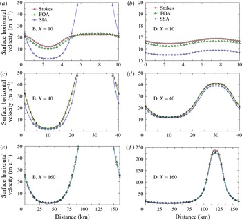
Stokes, Blatter, SSA and SIA surface horizontal velocities for ISMIP-HOM experiments B (a,c,e) and D ((b,d,f) with
 $X=10$
(a,b), 40 (c,d) and 160 km (e,f).

The set-ups of ISMIP-HOM experiments B and D show no lateral (in
 $y$
) variation in the boundary conditions and the geometry of the ice domain. Consequently, the velocity field is computed via a two-dimensional model. More precisely, in experiment B the geometry is defined by a flat inclined upper surface and a sinusoidal bed,
 $$\begin{eqnarray}\displaystyle \overline{s}(x) & = & \displaystyle -x\tan (0.5^{\circ }),\quad x\in [0,X],\end{eqnarray}$$
 $$\begin{eqnarray}\displaystyle \text{}\underline{s}(x) & = & \displaystyle \overline{s}(x)-1000+500\sin (2\unicode[STIX]{x03C0}x/X),\quad x\in [0,X],\end{eqnarray}$$
and a no-slip condition is prescribed on the bedrock, while in experiment D the geometry is defined by an inclined slab,
 $$\begin{eqnarray}\displaystyle \overline{s}(x) & = & \displaystyle -x\tan (0.1^{\circ }),\quad x\in [0,X],\end{eqnarray}$$
 $$\begin{eqnarray}\displaystyle \text{}\underline{s}(x) & = & \displaystyle \overline{s}(x)-1000,\quad x\in [0,X],\end{eqnarray}$$
and a slip condition everywhere on the bedrock defined by exponent
 $s=2$
in (2.10). It should be noted that choosing
 $s=2$
does not fulfil the theoretical requirement
 $s\in (1,p]$
since
 $p=4/3$
, and the coefficient in (2.10) is given by
 $$\begin{eqnarray}\displaystyle C(x)=1000(1+\sin (2\unicode[STIX]{x03C0}x/X)), & & \displaystyle\end{eqnarray}$$
where
 $X>0$
is the length of the domain. In both experiments, periodic boundary conditions connect the left- and right-hand sides of the domain
 $[0,X]$
, and a stress-free condition is prescribed on the top surface; see Pattyn et al. (Reference Pattyn2008) for further details on the model setting.
In order to assess the estimators in Theorem 1, we generally need all model solutions from SIA to Stokes. However, the SSA solution is not considered for experiment B because it gives identically zero velocity if there is no sliding. Likewise, the SIA solution is not considered for experiment D because SIA-type sliding is not allowed (as it is non-physical (Greve & Blatter Reference Greve and Blatter2009)).
The SIA solution is computed from its analytical form (Greve & Blatter Reference Greve and Blatter2009). The SSA and Blatter solutions are solved numerically using the Newton multigrid solver described in Jouvet & Gräser (Reference Jouvet and Gräser2013). The Stokes solutions are computed via the Elmer code (Gagliardini & Zwinger Reference Gagliardini and Zwinger2008). In all cases, one uses a 2D mesh extruded from a subdivision of the horizontal segment
 $[0,X]$
into 64 equal-sized segments with 16 uniformly distributed layers (except for the SSA which has a single layer). The numerical error in the solutions was assessed by examining the discrepancy between these solutions and those obtained by doubling the horizontal resolution and the number of layers. In order to obtain a wide range of aspect ratios, we ran both experiments (B and D) for several values of the domain length
 $X$
(
 $=$
5, 10, 20, 40, 80 and 160 km), giving corresponding values of the aspect ratio
 $\unicode[STIX]{x1D716}$
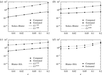
. Figure 4 shows the computed and estimated (estimators of Theorem 1) norm differences (normalized) between the Stokes–Blatter, Blatter–SIA and Blatter–SSA solutions of the ISMIP-HOM B and D experiments.
Computed and estimated (estimators of Theorem 1) norm differences (normalized) between ISMIP-HOM solutions versus the aspect ratio
 $\unicode[STIX]{x1D716}$
. The ‘computed’ (respectively ‘estimated’) norm difference corresponds to (a,c) (respectively b,d) of estimators (3.1)–(3.4) taking
 $c=c_{p}=c_{k}=1$
. Panel (a) (respectively b) concerns the Stokes–Blatter solution discrepancy for experiment B (respectively D). Panel (c) (respectively d) concerns the Blatter–SIA (respectively Blatter–SSA) solution discrepancy for experiment B (respectively D). Except for (d), regression straight lines have been drawn to compare the orders of convergence of the computed and estimated norm differences as a function of the aspect ratio.

As expected, figure 4 confirms that the Blatter solution converges to the Stokes solution, while the SIA and SSA converge to Blatter when the aspect ratio
 $\unicode[STIX]{x1D716}$
shrinks to zero. In fact, figure 4 shows that all of the computed errors and their estimators decrease in a similar way to zero (except between Blatter and SSA for ISMIP-HOM D). This validates the conclusions of Theorem 1 and its estimators (3.1)–(3.4) even in the presence of numerical approximations. The Stokes–Blatter estimator for ISMIP-HOM D is not dealt with in Theorem 1 since it assumes no basal sliding (
 $\unicode[STIX]{x1D6E4}_{m}=\emptyset$
). More precisely, the estimator (3.4) correctly predicts the
 ${\sim}O(\unicode[STIX]{x1D716}^{1.4})$
convergence of the mismatch between Stokes and Blatter in the no-sliding experiment ISMIP-HOM B. In addition, the estimator (3.3) gives the
 ${\sim}O(\unicode[STIX]{x1D716}^{0.7})$
convergence of the norm difference between Blatter and SIA in the same experiment. Interestingly, the power of
 $\unicode[STIX]{x1D716}$
is halved between the two solutions, in agreement with the construction of each model: the SIA truncates terms with an order higher than 0 while the Blatter solution truncates terms with an order higher than 1 (with respect to
 $\unicode[STIX]{x1D716}$
). However, figure 4 also shows that the order of convergence of the discrepancy between Stokes and Blatter is not intrinsic, but depends on the type of ice flow. Indeed, this convergence drops to
 ${\sim}O(\unicode[STIX]{x1D716}^{0.4})$
in the sliding-dominant experiment ISMIP-HOM D. One can explain the weakening of the convergence by the fact that the vertical velocities become negligible more rapidly in the sliding-dominant experiment compared with the no-sliding experiment on decreasing the aspect ratio
 $\unicode[STIX]{x1D716}$
. However, the estimator (3.4) shows a higher rate of convergence. This confirms that this estimator is not appropriate when prescribing basal sliding, a fact already suggested by Theorem 1 and its proof; see Remark 3.38. Finally, figure 4 shows that both the norm difference between SSA and Blatter and its estimator (3.1) decrease similarly to zero in the sliding-dominant experiment ISMIP-HOM D. In contrast to other cases, the convergence Blatter–SSA shows a nonlinear behaviour. The convergence is faster at high aspect ratios, but slows down on decreasing the aspect ratio.
5 Conclusion
In the literature, shallow ice flow models are traditionally obtained from the strong form of the Glen–Stokes equations. In this paper, the construction of these models has instead been assessed by working in the weak (or variational) form. By doing so, the pressure, a Lagrange multiplier for the incompressibility condition, does not appear explicitly in the reduced variational form. As a consequence, no ‘hydrostatic approximation’ assumption is needed to eliminate the pressure (Dukowicz Reference Dukowicz2012) as in the derivation of the Blatter model, with the result that the overall model construction becomes simpler. Another advantage of this approach is that it leads to a unified and variational formulation of shallow ice flow models. This made it possible to derive error estimators that can predict the accuracy of any shallow ice model as compared with its immediate predecessor. To do this, techniques were followed that have been used elsewhere to obtain a posteriori estimators of the numerical error. As a result, our estimators involve residuals (i.e. terms that were neglected in the model derivation, but that are evaluated here from the simplified model solution) to measure the discrepancy between two embedded model solutions. The reliability of our estimators was validated by performing two modelling ISMIP-HOM experiments, which involve various types of ice flow (no sliding and sliding-dominant). Our estimates were able to predict the non-trivial decay of the discrepancy between the model solutions on decreasing the aspect ratio for most of the experiments.
Although the estimates we have derived in this study give only a global measure of the discrepancy between model solutions (i.e. integrated over the entire domain of ice), the techniques used remain valid to obtain similar but local estimates (i.e. integrated on a given subdomain) provided that there are Dirichlet and/or Neumann conditions on the boundary of the subdomain. Such local estimators could have a relevant application in multimodel approaches, see, e.g., Seroussi (Reference Seroussi2011) and Ahlkrona et al. (Reference Ahlkrona, Lotstedt, Kirchner and Zwinger2016), since they can be used to assign suitable ice flow models to subdomains in an optimal, rather than empirical, way. Another aspect to investigate is the use of mechanical estimators for preconditioning purposes. Indeed, the estimators (3.3) and (3.1) could perhaps be used to determine the local features of the ice flow (from shearing to sliding-dominant), and this information could be exploited to efficiently precondition the matrices resulting from the Blatter discretization (Brown, Smith & Ahmadia Reference Brown, Smith and Ahmadia2013).
Acknowledgements
The author wishes to acknowledge E. Bueler, C. Schoof and an anonymous referee for their detailed and helpful comments on the manuscript, M. Picasso for his help in proving estimator (3.1), and S. Braun-Clarke for proofreading the English.