1 Introduction
The study of fluid turbulence connects bulk statistical properties such as energy spectra, structure functions, and the energy dissipation rate to physical processes such as vortex stretching and instabilities (Frisch Reference Frisch1995). In the context of geophysical turbulence, the emphasis is on how rotation and density stratification affect the statistical and dynamical properties of the turbulent flow. At small scales, rotation and buoyancy are expected to become dynamically unimportant, with statistics resembling those of non-rotating, constant-density flow. More specifically, rotation and buoyancy, respectively, are expected to become unimportant for scales smaller than the Zeman scale
 $L_{{\it\Omega}}=\sqrt{{\it\epsilon}/(2{\it\Omega})^{3}}$
(Zeman Reference Zeman1994) and the Ozmidov scale
 $L_{N}=\sqrt{{\it\epsilon}/N^{3}}$
(Ozmidov Reference Ozmidov1965), where
 ${\it\epsilon}$
is the mean rate of energy dissipation per unit mass,
 ${\it\Omega}$
is the rate of rotation, and
 $N=\sqrt{-g\partial _{z}{\it\rho}/{\it\rho}_{0}}$
is the buoyancy frequency in a density-stratified fluid under the Boussinesq approximation (
 $g$
is the gravitational acceleration,
 ${\it\rho}$
is the density, and
 ${\it\rho}_{0}$
is a constant reference density). Studies of geophysical turbulence therefore include scales larger than either the Ozmidov or Zeman scales, or both.
The presence of system rotation and density stratification each induce restoring forces that lead to wave dynamics. In the special case where the rotation vector is parallel to gravity, the linear wave frequencies vary between the values
 $N$
and
 $2{\it\Omega}$
. Effects of system rotation and density stratification are expected to have a qualitative impact on turbulence when the period of wave dynamics is comparable to or less than the time scale of nonlinear advection. More precisely, rotation and stratification, respectively, are expected to strongly affect the dynamics when the Rossby number
 $Ro=U/(2{\it\Omega}L)$
and Froude number
 $Fr=U/(NL)$
are small, where
 $U$
and
 $L$
are characteristic velocity and length scales of the turbulent flow. Geophysical turbulence is characterized by small Rossby and/or Froude numbers.
The linear eigenfunctions of the Boussinesq system include two wave modes and a zero-frequency ‘vortical’ mode (Bartello Reference Bartello1995). At low Rossby and Froude numbers, there is a clear time scale separation between the slow, nonlinear evolution of the vortical mode and the fast, weakly nonlinear evolution of the wave modes, which can be exploited to derive asymptotically a reduced set of dynamics for the vortical modes; this reduced system is the celebrated quasi-geostrophic equations (Charney Reference Charney1948; Eady Reference Eady1949; Pedlosky Reference Pedlosky1987; Vallis Reference Vallis2006). Bartello (Reference Bartello1995) argued on the basis of statistical mechanics and demonstrated, using numerical simulations, that in the low-Rossby-number, low-Froude-number limit the vortical mode evolution is not influenced by the wave modes and that the freely evolving dynamics will eventually approach a state of quasi-geostrophic balance. Time scale separation was exploited by Embid and Majda to rigorously prove the validity of the quasi-geostrophic system even in the presence of wave modes with amplitudes comparable to the vortical modes, in contrast to the asymptotic derivation which assumes that any waves have low amplitude (Embid & Majda Reference Embid and Majda1996, Reference Embid and Majda1998; Majda & Embid Reference Majda and Embid1998). Temam & Wirosoetisno (Reference Temam and Wirosoetisno2010, Reference Temam and Wirosoetisno2011) have also proved rigorously that, under mild assumptions, the small-Rossby-number, small-Froude-number dynamics eventually approaches a quasi-geostrophic balance irrespective of the amplitude of wave modes in the initial condition (this result was obtained under the hydrostatic approximation). The quasi-geostrophic system is thus a natural touchstone for geophysical turbulence, and the qualitative properties of turbulence in the quasi-geostrophic system were presciently forecast by Charney (Reference Charney1971) based on an analogy with previous studies of two-dimensional turbulence.
The rigorous framework of Embid & Majda (Reference Embid and Majda1996) exploits an asymptotic time scale separation between the fast wave dynamics and the slow ‘balanced’ dynamics. Embid & Majda (Reference Embid and Majda1998) and Wingate et al. (Reference Wingate, Embid, Holmes-Cerfon and Taylor2011) also used the framework to rigorously derive equations governing the slow limiting dynamics in the limits of low Froude and finite Rossby numbers, and low Rossby and finite Froude numbers, respectively. Because of the a priori need for an asymptotic time scale separation, the slow limiting dynamics include a single pair of wave modes at the slowest linear frequency (
 $2{\it\Omega}$
for Embid & Majda (Reference Embid and Majda1998) and
 $N$
for Wingate et al. (Reference Wingate, Embid, Holmes-Cerfon and Taylor2011)), and all other wave modes are assumed to be asymptotically fast by comparison, and do not appear in the slow limiting dynamics. Results analogous to those of Temam & Wirosoetisno (Reference Temam and Wirosoetisno2010) for the quasi-geostrophic system are lacking for these two systems of slow limiting dynamics, and it is not yet clear whether these systems have the same relevance for geophysical turbulence in their respective asymptotic regimes as the quasi-geostrophic system has for the low-Froude-number, low-Rossby-number regime.
If either the Rossby or Froude number is order-one, there is no clear time scale separation between the linear wave dynamics and the nonlinear advective dynamics, so a reduced system that eliminates nearly all the wave dynamics is arguably inappropriate. Nevertheless, the smallness of one of the non-dimensional numbers can still be exploited in both cases to reduce the complexity of the full Boussinesq system. When the Froude number is small but the Rossby number is order-one, one can make the hydrostatic approximation to arrive at the so-called primitive equations. When the Rossby number is small but the Froude number is order-one, one can make a geostrophic approximation and arrive at the non-hydrostatic quasi-geostrophic equations (NHQGE; Julien, Knobloch & Werne Reference Julien, Knobloch and Werne1998; Julien et al.
Reference Julien, Knobloch, Milliff and Werne2006). Both of these equation sets are significantly easier for numerical simulation than the unreduced Boussinesq equations, and both sets of equations include linear wave dynamics with frequencies between either
 $2{\it\Omega}$
(primitive equations) or
 $N$
(NHQGE) and infinity. The quasi-geostrophic equations can be recovered from both sets of equations in the limit where both the Rossby and Froude numbers are small. While it is difficult to obtain rigorous mathematical results using the Boussinesq equations, Temam & Wirosoetisno (Reference Temam and Wirosoetisno2010) were able to obtain useful rigorous results starting from the simpler hydrostatic equations. It may be the case that similar rigorous results may be obtained for a different complementary parameter regime using the non-hydrostatic quasi-geostrophic equations.
As the Froude number is typically smaller than the Rossby number in atmospheric and oceanic turbulence, studies of rotating, stratified turbulence have primarily focused on strongly stratified regimes where the Froude number is small. The regime of geostrophic turbulence with low Rossby number and order-one Froude number has seen comparatively little study, though this regime may be relevant to weakly stratified abyssal ocean dynamics at high latitudes and in the western Mediterranean (Emery, Lee & Magaard Reference Emery, Lee and Magaard1984; Timmermans, Garrett & Carmack Reference Timmermans, Garrett and Carmack2003; van Haren & Millot Reference van Haren and Millot2005; Timmermans, Melling & Rainville Reference Timmermans, Melling and Rainville2007). The regime is also relevant to planetary and stellar interiors where the stratification transitions from unstable (imaginary
 $N$
) to stable (
 $N\geqslant 0$
). Examples include the solar tachocline, believed to be the origin of large-scale solar magnetism (Miesch Reference Miesch2005), and the Earth’s outer liquid core, where the existence of stably stratified layers have been postulated (Pozzo et al.
Reference Pozzo, Davies, Gubbins and Alfè2012). The present investigation focuses on rotating, stratified turbulence at low Rossby number, with Froude numbers varying from large to small.
The main points of comparison for the transitional regime of Froude numbers between zero and infinite are the ‘quasi-geostrophic’ regime at small Froude numbers and pure rotation at large Froude numbers. Quasi-geostrophic turbulence theory, by analogy with the theory of two-dimensional turbulence, predicts a transfer of energy from the forcing scale to larger scales through an inertial range where the energy spectrum is proportional to
 $\tilde{k}^{-5/3}$
, where
 $\tilde{k}^{2}=k_{h}^{2}+(2{\it\Omega}/N)^{2}k_{z}^{2}$
(Charney Reference Charney1971; Boffetta & Ecke Reference Boffetta and Ecke2012). At scales smaller than the energy forcing, quasi-geostrophic turbulence theory predicts an energy spectrum proportional to
 $\tilde{k}^{-3}$
. The
 $-5/3$
(Smith & Waleffe Reference Smith and Waleffe2002; Marino et al.
Reference Marino, Mininni, Rosenberg and Pouquet2013) and
 $-3$
(Waite & Bartello Reference Waite and Bartello2006) spectral slopes are evident in simulations of triply periodic Boussinesq dynamics in the regime of low Rossby and Froude numbers, and both Waite & Bartello (Reference Waite and Bartello2006) and Whitehead & Wingate (Reference Whitehead and Wingate2014) observed energy accumulating in the vortical modes. These results underscore the importance of quasi-geostrophic dynamics, and demonstrate that the theorem of Temam & Wirosoetisno (Reference Temam and Wirosoetisno2010) applies qualitatively even in this stochastically forced regime.
In simulations of constant-density (infinite Froude number), low-Rossby-number turbulence, energy is transferred to scales larger than the forcing scale through an inertial range with spectrum proportional to
 $k^{-3}$
; energy is also primarily transferred to a depth-independent horizontal velocity, the ‘barotropic mode’ (Smith & Waleffe Reference Smith and Waleffe1999; Smith & Lee Reference Smith and Lee2005). Marino et al. (Reference Marino, Mininni, Rosenberg and Pouquet2013) found transfer of energy into the barotropic mode to be less rapid in the purely rotating regime than in the quasi-geostrophic regime. Sen et al. (Reference Sen, Mininni, Rosenberg and Pouquet2012) observed a
 $k^{-5/3}$
spectrum at large scales in a purely rotating system when the stochastic forcing was independent of depth; this case is somewhat degenerate and likely not indicative of universal behaviour.
The transitional regime between pure rotation and quasi-geostrophy has seen comparatively few simulations. In the simulations of Sukhatme & Smith (Reference Sukhatme and Smith2008), the Froude and Rossby numbers are both comparatively small, though in some simulations the Froude number was larger by up to a factor of five. In their simulations with Froude number larger than Rossby number, the wave mode energy grows to dominate, in contrast to the behaviour in both the quasi-geostrophic and purely rotating limits, where energy accumulates primarily in the vortical and depth-independent components; this may be related to the fact that forcing was applied near the scale of the computational domain. They found that the vortical mode spectrum retained its quasi-geostrophic
 $k^{-3}$
behaviour at scales smaller than the forcing, though it deviated towards a shallower slope at much smaller scales. In a single experiment with low Rossby number and moderate Froude number, also forced near the scale of the computational domain, Aluie & Kurien (Reference Aluie and Kurien2011) diagnosed a downscale transfer of both energy and potential enstrophy; spectral slopes were not reported. Whitehead & Wingate (Reference Whitehead and Wingate2014) also forced near the scale of the computational box, and found energy accumulating in the barotropic mode; spectral slopes were not reported. These investigations leave open entirely the question of how the large-scale dynamics transition between the quasi-geostrophic and purely rotating regimes as the Froude number increases, which is the focus of the present investigation.
The paper is organized as follows: § 2 introduces preliminaries, including discussions regarding Proudman–Taylor constraints and inertia-gravity waves; § 3 provides an overview of the reduced equations used in our numerical simulations; § 4 summarizes the numerical methods, including the forcing scheme employed for numerical simulations; and § 5 gives the results of our numerical experiments.
2 Governing equations and preliminaries
We consider an incompressible fluid subject to an imposed constant vertical gravitational field
 $\boldsymbol{g}=-g\hat{\boldsymbol{z}}$
and a system rotation with constant angular velocity
 ${\it\bf\Omega}={\it\Omega}\hat{\boldsymbol{z}}$
. The fluid is stably stratified in the vertical with total density
 ${\it\rho}^{\ast }=\hat{{\it\rho}}^{\ast }(z^{\ast })+{{\it\rho}^{\prime }}^{\ast }(\boldsymbol{x}^{\ast },t^{\ast })$
, where
 $\hat{{\it\rho}}^{\ast }(z^{\ast })={\it\rho}_{0}^{\ast }+{\it\delta}\hat{{\it\rho}}^{\ast }(z^{\ast })$
is an ambient density profile consisting of a constant reference density
 ${\it\rho}_{0}^{\ast }$
and a density variation
 ${\it\delta}\hat{{\it\rho}}^{\ast }(z^{\ast })$
(where asterisks denote dimensional quantities). It follows that the total buoyancy of a fluid parcel, given by
 $$\begin{eqnarray}b^{\ast }=-\frac{g}{{\it\rho}_{0}^{\ast }}({\it\delta}\hat{{\it\rho}}^{\ast }(z^{\ast })+{{\it\rho}^{\prime }}^{\ast }(\boldsymbol{x}^{\ast },t^{\ast }))=-\frac{g}{{\it\rho}_{0}^{\ast }}{\it\delta}\hat{{\it\rho}}^{\ast }(z^{\ast })+b^{\ast \prime }(\boldsymbol{x}^{\ast },t^{\ast }),\end{eqnarray}$$
is decomposed as the sum of the ambient buoyancy field and a fluctuating component
 $b^{\ast \prime }$
associated with fluid motions. Pressure is decomposed in a fashion similar to buoyancy
 $p^{\ast }=\hat{p}^{\ast }(z^{\ast })+{p^{\prime }}^{\ast }(\boldsymbol{x}^{\ast },t^{\ast })$
, with a pressure component in hydrostatic balance with the ambient buoyancy
 $$\begin{eqnarray}\partial _{z^{\ast }}{\it\delta}\hat{p}^{\ast }(z^{\ast })=-g\hat{{\it\rho}}^{\ast }(z^{\ast }).\end{eqnarray}$$
The governing equations in the Boussinesq approximation for a fluid with constant kinematic viscosity
 ${\it\nu}$
and buoyancy diffusion
 ${\it\kappa}$
are given by
 $$\begin{eqnarray}\displaystyle D_{t}^{\ast }\boldsymbol{u}^{\ast }+2{\it\Omega}\hat{\boldsymbol{z}}\times \boldsymbol{u}^{\ast } & = & \displaystyle -\boldsymbol{{\rm\nabla}}p^{\ast \prime }+b^{\ast \prime }\hat{\boldsymbol{z}}+{\it\nu}{\rm\nabla}^{\ast 2}\boldsymbol{u}^{\ast },\end{eqnarray}$$
 $$\begin{eqnarray}\displaystyle D_{t}^{\ast }b^{\ast \prime }+N^{2}(z^{\ast })w^{\ast } & = & \displaystyle {\it\kappa}{\rm\nabla}^{\ast 2}b^{\ast \prime },\end{eqnarray}$$
 $$\begin{eqnarray}\displaystyle \boldsymbol{{\rm\nabla}}^{\ast }\boldsymbol{\cdot }\boldsymbol{u}^{\ast } & = & \displaystyle 0,\end{eqnarray}$$
 $$\begin{eqnarray}D_{t}^{\ast }(\cdot )=[\partial _{t^{\ast }}+\boldsymbol{u}^{\ast }\boldsymbol{\cdot }\boldsymbol{{\rm\nabla}}^{\ast }](\cdot ).\end{eqnarray}$$
The ambient stratification is now characterized by the buoyancy (Brunt–Väisälä) frequency
 $N^{2}(z^{\ast })=-g{\it\rho}_{0}^{\ast -1}\partial _{z^{\ast }}({\it\delta}\hat{{\it\rho}}^{\ast }(z^{\ast }))$
.
An external forcing is required to excite fluid motions, and in the present investigation energy is generated by a stochastic vertical velocity forcing. Recent studies in a similar parameter regime have used stochastic buoyancy forcing (Whitehead & Wingate Reference Whitehead and Wingate2014) or simultaneous forcing of all components of velocity (Marino et al. Reference Marino, Mininni, Rosenberg and Pouquet2013). The present investigation includes regimes of weak stratification (large Froude numbers) and the presence of inertia-gravity waves with external forcing that is intended to represent a source of baroclinic motion in a fluid replete with wave energy. Initial tests with buoyancy forcing in the weakly stratified regime led to frequent large-scale overturning. Vertical velocity forcing avoids these spurious dynamics in the weakly stratified regime while also avoiding direct forcing of the slow quasi-geostrophic dynamics in the strongly stratified regime.
Characteristic scales determined from the energy injection rate
 ${\it\epsilon}_{f}^{\ast }$
and forcing length scale
 $L_{f}^{\ast }$
are the forcing velocity, time and buoyancy scales
 $$\begin{eqnarray}U_{f}^{\ast }=({\it\epsilon}_{f}^{\ast }L_{f}^{\ast })^{1/3},\quad T_{f}^{\ast }=(L_{f}^{\ast 2}{\it\epsilon}_{f}^{\ast -1})^{1/3},\quad B_{f}^{\ast }=({\it\epsilon}_{f}^{\ast 2}L_{f}^{\ast -1})^{1/3}.\end{eqnarray}$$
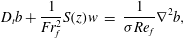
This gives rise to the following non-dimensional equations
 $$\begin{eqnarray}\displaystyle D_{t}\boldsymbol{u}+\frac{1}{Ro_{f}}\hat{\boldsymbol{z}}\times \boldsymbol{u} & = & \displaystyle -Eu_{f}\boldsymbol{{\rm\nabla}}p+b\hat{\boldsymbol{z}}+\frac{1}{Re_{f}}{\rm\nabla}^{2}\boldsymbol{u},\end{eqnarray}$$
 $$\begin{eqnarray}\displaystyle D_{t}b+\frac{1}{Fr_{f}^{2}}S(z)w & = & \displaystyle \frac{1}{{\it\sigma}Re_{f}}{\rm\nabla}^{2}b,\end{eqnarray}$$
 $$\begin{eqnarray}\displaystyle \boldsymbol{{\rm\nabla}}\boldsymbol{\cdot }\boldsymbol{u} & = & \displaystyle 0,\end{eqnarray}$$
 $$\begin{eqnarray}D_{t}(\cdot )=[\partial _{t}+\boldsymbol{u}\boldsymbol{\cdot }\boldsymbol{{\rm\nabla}}](\cdot )\end{eqnarray}$$
and
 $S(z)$
is the non-dimensional stratification profile defined according to the relation
 $N^{2}(z^{\ast })=N_{0}^{2}S(z)$
. We have defined
 $N_{0}\equiv |g{\it\rho}_{0}^{\ast -1}(\partial _{z^{\ast }}{\it\delta}\hat{{\it\rho}}^{\ast }(z^{\ast }))_{max}|$
as the maximal buoyancy frequency and
 $S\equiv -\partial _{z}{\it\delta}\hat{{\it\rho}}$
.
The non-dimensional parameters that appear in (2.6) are determined a priori based on the energy injection rate
 ${\it\epsilon}_{f}^{\ast }$
and forcing length scale
 $L_{f}^{\ast }$
. These parameters are the Rossby number
 $Ro_{f}$
, Froude number
 $Fr_{f}$
, Euler number
 $Eu_{f}$
, and Reynolds number
 $Re_{f}$
, defined as
 $$\begin{eqnarray}Ro_{f}=\frac{U_{f}^{\ast }}{2{\it\Omega}L_{f}^{\ast }},\quad Fr_{f}=\frac{U_{f}^{\ast }}{N_{0}L_{f}^{\ast }},\quad Eu_{f}=\frac{{\it\delta}p_{0}}{{\it\rho}_{0}U_{f}^{\ast 2}},\quad Re_{f}=\frac{U_{f}^{\ast }L_{f}^{\ast }}{{\it\nu}}\equiv \left(\frac{{\it\epsilon}_{f}^{\ast }L_{f}^{\ast 4}}{{\it\nu}^{3}}\right)^{1/3}.\end{eqnarray}$$
The Rossby number is the ratio of rotation period,
 $T_{{\it\Omega}}^{\ast }=1/2{\it\Omega}$
, to the forcing time,
 $T_{f}^{\ast }=L_{f}^{\ast }/U_{f}^{\ast }$
, and measures the rotational constraint of the fluid at the forcing scale. Hereafter, we focus solely on the rotationally constrained regime
 $Ro_{f}\ll 1$
. The Froude number is the ratio of the Brunt–Väisälä time,
 $T_{N}^{\ast }=1/N_{0}$
, to
 $T_{f}^{\ast }$
and measures the ratio of the fastest linear wave period to the nonlinear advective time scale. The Reynolds number provides a non-dimensional measure of the energy injection rate into the system and therefore controls the degree of turbulence achieved at the forcing scale
 $L_{f}^{\ast }$
. The Euler number measures the significance of the pressure gradient force relative to inertial accelerations. The Prandtl number
 ${\it\sigma}={\it\nu}/{\it\kappa}$
is the ratio of dissipation parameters and quantifies the thermometric properties of the working fluid.
In addition to the non-dimensional forcing length scale
 $L_{f}=1$
, four internal length scales are also present: the dissipation (Kolmogorov) scale
 $L_{K}$
, first Rossby radius of deformation
 $L_{D}$
, the Zeman length scale
 $L_{{\it\Omega}}$
, and the Ozimodov length scale
 $L_{N}$
. These non-dimensional length scales are defined, respectively, as
 $$\begin{eqnarray}L_{K}\equiv Re_{f}^{-3/4},\quad L_{D}\equiv \left(\frac{N_{0}H^{\ast }}{2{\it\Omega}L_{f}^{\ast }}\right)=\frac{ARo_{f}}{Fr_{f}},\end{eqnarray}$$
 $$\begin{eqnarray}L_{{\it\Omega}}\equiv \left(\frac{{\it\epsilon}_{f}^{\ast }L_{f}^{\ast -2}}{(2{\it\Omega})^{3}}\right)^{1/2}=Ro_{f}^{3/2}\ll 1,\quad L_{N}\equiv \displaystyle \left(\frac{{\it\epsilon}_{f}^{\ast }L_{f}^{\ast -2}}{N_{0}^{3}}\right)^{1/2}=Fr_{f}^{3/2}.\end{eqnarray}$$
The dissipation scale is the scale at which the nonlinear turnover time equals the time scale of viscous dissipation. The first Rossby radius of deformation is the scale where baroclinic instability converts potential to kinetic energy, and depends on
 $H^{\ast }$
, the depth of the domain. The ratio
 $A=H^{\ast }/L_{f}^{\ast }$
is the non-dimensional height of the domain, and is set a priori when
 $Ro_{f}\ll 1$
(see § 2.1 below). In quasi-geostrophic dynamics the conversion of baroclinic to barotropic energy (we adopt the convention that the ‘barotropic’ component of the system includes only the depth-independent part of the horizontal velocity; all other fields including vertical velocity and buoyancy are ‘baroclinic’) occurs mainly at scales larger than
 $L_{D}$
. Rotation influences the dynamics at scales larger than the Zeman scale, and the Ozimodov scale is that above which eddies are influenced by stratification.
In this paper, we consider only the case
 $L_{{\it\Omega}}<L_{K}$
such that all fluid scales are influenced by rotation. This constraint places an upper bound for the Rossby number, namely
 $$\begin{eqnarray}Ro_{f}\ll Re_{f}^{-1/2}.\end{eqnarray}$$
This relation can also be interpreted as placing an upper bound on the Reynolds number; at sufficiently large Reynolds numbers the Zeman scale would be larger than the Kolmogorov scale, indicating a transition from rotationally dominated to isotropic turbulence at scales larger than the dissipation scale (e.g. Mininni, Rosenberg & Pouquet Reference Mininni, Rosenberg and Pouquet2012). Strongly stratified non-rotating turbulence displays marked qualitative differences, depending on the relative size of the Ozmidov and Kolmogorov length scales (Waite & Bartello Reference Waite and Bartello2004; Brethouwer et al.
Reference Brethouwer, Billant, Lindborg and Chomaz2007); it remains to be seen whether the qualitative results we obtain under the assumption
 $L_{{\it\Omega}}<L_{K}$
change for rapidly rotating flows with
 $L_{{\it\Omega}}\geqslant L_{K}$
. Given that the Rossby number is very small and the Euler number passively scales pressure, it becomes clear that there exist two primary control parameters,
 $Re_{f}$
and
 $Fr_{f}$
. Varying these parameters causes the three dynamical length scales,
 $L_{D}$
,
 $L_{N}$
and
 $L_{K}$
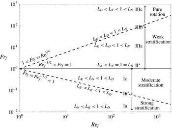
to vary through the seven distinct regimes shown in figure 1.
Distinguished parameter regimes from strong stratification (Ia) to weak stratification (IIIc).
 $\ast =\text{boundary regimes}$
. In all cases the Zeman scale is smaller than the Kolmogorov scale; i.e.
 $Re_{f}\ll Ro_{f}^{-2}$
.

2.1 Geostrophy and the Proudman–Taylor constraint
The Proudman–Taylor constraint on rapidly rotating fluids arises from the curl of the non-dimensional momentum equations (2.6a )
 $$\begin{eqnarray}D_{t}{\bf\omega}=\left({\bf\omega}+\frac{1}{Ro_{f}}\hat{\boldsymbol{z}}\right)\boldsymbol{\cdot }\boldsymbol{{\rm\nabla}}\boldsymbol{u}+\boldsymbol{{\rm\nabla}}\times b\hat{\boldsymbol{z}}+\frac{1}{Re_{f}}{\rm\nabla}^{2}{\bf\omega},\end{eqnarray}$$
where
 ${\bf\omega}=\boldsymbol{{\rm\nabla}}\times \boldsymbol{u}$
(Proudman Reference Proudman1916; Taylor Reference Taylor1923; Greenspan Reference Greenspan1968). The leading-order balance at small Rossby numbers is simply
 $\partial _{z}\boldsymbol{u}=0$
. This leading-order balance can be broken if any of the remaining terms in the vorticity equation rise to order
 $Ro_{f}^{-1}$
; for example, the Proudman–Taylor constraint can be broken in thin viscous boundary layers. A more relevant example is the quasi-geostrophic regime, where the curl of the buoyancy force is sufficiently large to result in the thermal-wind balance at leading order
 $$\begin{eqnarray}-\partial _{z}\boldsymbol{u}=\boldsymbol{{\rm\nabla}}\times b\hat{\boldsymbol{z}}.\end{eqnarray}$$
The leading-order asymptotic balance associated with the Proudman–Taylor constraint can be more usefully written as
 $$\begin{eqnarray}\partial _{z}\boldsymbol{u}=O(Ro_{f}),\end{eqnarray}$$
which suggests that the Proudman–Taylor constraint can be broken by allowing variation in the
 $\hat{\boldsymbol{z}}$
direction on vertical scales order
 $Ro_{f}^{-1}$
larger than the horizontal scales of motion, i.e., by allowing
 $A=H^{\ast }/L_{f}^{\ast }=Ro_{f}^{-1}$
(as is done in the present study). In summary, for weak buoyancy, associated with weak stratification, one expects the dynamics to be tall and thin, whereas for strong buoyancy and strong stratification one expects the dynamics to display an order-one aspect ratio. The equations used in our numerical experiments (described in § 3) are geostrophically balanced, yet break the Proudman–Taylor constraint at small horizontal scales by allowing long vertical variations. The equations also allow the Proudman–Taylor constraint to be broken on unit-aspect-ratio scales in the presence of sufficiently strong buoyancy forcing.
2.2 Eddy–wave dispersion relation at
 $Ro_{f}\ll 1$

A linear analysis of the unforced and inviscid form of (2.6), for normal modes
 $\propto \exp [\text{i}({\it\omega}t+\boldsymbol{k}_{\bot }\boldsymbol{\cdot }\boldsymbol{x}_{\bot }+k_{z}z)]$
, provides the inertia-gravity dispersion relation for the wave frequency of oscillation
 ${\it\omega}$
and the horizontal and vertical wavenumbers
 $\boldsymbol{k}_{\bot },k_{z}$
:
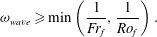
 $$\begin{eqnarray}{\it\omega}_{wave}^{2}=\frac{1}{Fr_{f}^{2}}\sin ^{2}{\it\theta}+\frac{1}{Ro_{f}^{2}}\cos ^{2}{\it\theta},\quad {\it\omega}_{eddy}^{2}=0.\end{eqnarray}$$
Here
 ${\it\theta}=\tan ^{-1}(k_{\bot }/k_{z})$
denotes the angle made with the positive
 $\boldsymbol{z}$
-axis. The dispersion relation (2.15) implies the following bound on the wave frequencies
 $$\begin{eqnarray}{\it\omega}_{wave}\geqslant \min \left(\frac{1}{Fr_{f}},\frac{1}{Ro_{f}}\right).\end{eqnarray}$$
In the following we consider the wave dispersion relation (2.15) in the limit
 $Ro_{f}~\ll ~1$
as a function of stratification which, as established in the previous section, is tied to the spatial anisotropy of the flow. In addition to
 $Ro_{f}\ll 1$
, if stratification is strong (i.e., if
 $Fr_{f}\ll 1$
), then the wave dispersion relation implies
 ${\it\omega}_{wave}\gg 1$
for all
 ${\it\theta}$
. Hence wave and eddy-turnover time scales are asymptotically separated for all waves. This is the classical quasi-geostrophic limit, where it is well established that fast inertia-gravity waves may be filtered from the Boussinesq equations. This reduction leads to the hydrostatic QG equations describing the evolution of eddies on a slow manifold.
In the case of weakly stratified flows characterized by
 $Fr_{f}=O(1)$
there are fast waves and slow waves, depending on the anisotropy of the wave, i.e.
 ${\it\theta}$
. The dispersion relation (2.15) clearly shows that waves with
 ${\it\theta}\sim \pm ({\rm\pi}/2-O(Ro_{f}))$
retain order-one frequencies in the limit
 $Ro_{f}\ll 1$
. Waves with angle
 ${\it\theta}\sim \pm ({\rm\pi}/2-O(Ro_{f}))$
have
 $k_{\bot }/k_{z}\sim Ro_{f}^{-1}$
, i.e. longer vertical than horizontal scales. It is now seen that these anisotropic inertia-gravity waves are not fast compared to the nonlinear eddy dynamics; since there is no gap between the time scale of waves and the time scale of eddies, the idea of a slow manifold is no longer applicable.
An approximate dispersion relation for these slow waves is obtained by inserting
 $k_{\bot }/k_{z}\sim Ro_{f}^{-1}$
into the dispersion relation (2.15) and eliminating small terms; the result is
 $$\begin{eqnarray}{\it\omega}_{wave}^{2}\sim \frac{1}{Fr_{f}^{2}}+\left(\frac{k_{z}}{k_{\bot }Ro_{f}}\right)^{2},\quad \frac{k_{z}}{k_{\bot }}\sim Ro_{f}.\end{eqnarray}$$
The phase and group velocities
 $\boldsymbol{v}_{p}$
and
 $\boldsymbol{v}_{g}$
associated with these slow waves are given by
 $$\begin{eqnarray}\displaystyle & \displaystyle \boldsymbol{v}_{p}\sim \frac{{\it\omega}_{wave}}{k_{\bot }^{2}}(k_{x},k_{y},k_{z})=O(1,1,Ro_{f}), & \displaystyle\end{eqnarray}$$
 $$\begin{eqnarray}\displaystyle & \displaystyle \boldsymbol{v}_{g}\sim \left(\frac{k_{z}}{k_{\bot }Ro_{f}}\right)^{2}\frac{1}{k_{\bot }^{2}{\it\omega}_{wave}}\left(-k_{x},-k_{y},\frac{k_{\bot }^{2}}{k_{z}}\right)=O(1,1,Ro_{f}^{-1}), & \displaystyle\end{eqnarray}$$
 $\boldsymbol{v}_{p}\boldsymbol{\cdot }\boldsymbol{v}_{g}=0$
and
 $|\boldsymbol{v}_{g}|\gg |\boldsymbol{v}_{p}|$
. Hence, inertia-gravity waves have phase and group velocities that are perpendicular: the slow waves propagate predominantly in horizontal directions whilst wave energy propagated by the group velocity is transmitted predominantly in the vertical direction (Greenspan Reference Greenspan1968). We note that velocity magnitudes are such that information is transmitted on the
 $O(1)$
eddy-turnover time in all directions; this follows from the fact that information in the horizontal propagates over
 $O(1)$
horizontal scales while information in the vertical propagates over
 $O(Ro_{f}^{-1})$
vertical scales. The consequences of wave–eddy interactions without a time scale separation are still not fully understood. In the following, we analyse and simulate reduced equations that describe the nonlinear interactions of vortical modes and slow inertia-gravity waves.
3 Reduced non-hydrostatic quasi-geostrophic equations
Detailed derivations of the NHQGE have been documented elsewhere (Julien et al.
Reference Julien, Knobloch, Milliff and Werne2006; Sprague et al.
Reference Sprague, Julien, Knobloch and Werne2006; Julien & Knobloch Reference Julien and Knobloch2007). In the following, we present the NHQGE, highlighting only the most salient points. Deduction of the NHQGE proceeds by identifying the Rossby number
 ${\it\varepsilon}\equiv Ro_{f}\ll 1$
as the small parameter and introducing the asymptotic series expansion
 $$\begin{eqnarray}\boldsymbol{v}=(\boldsymbol{u},p,b)^{T}={\it\varepsilon}^{-1}\boldsymbol{v}_{-1}+\boldsymbol{v}_{0}+{\it\varepsilon}\boldsymbol{v}_{1}+{\it\varepsilon}^{2}\boldsymbol{v}_{3}+O({\it\varepsilon}^{3})\end{eqnarray}$$
together with a multiple time scale expansion and a rescaled, anisotropic vertical coordinate
 $$\begin{eqnarray}\partial _{z}\rightarrow {\it\varepsilon}\partial _{Z},\quad \partial _{t}\rightarrow \partial _{t}+{\it\varepsilon}^{2}\partial _{T}\end{eqnarray}$$
into the Boussinesq equations. The large vertical scale is precisely the scale at which deviations from the Proudman–Taylor constraint are allowed. The slow dimensional time scale
 $T^{\ast }$
is the period over which the vertical buoyancy flux acts to modify the mean buoyancy profile, and is such that the ratio of the order-one time scale
 $T_{f}^{\ast }$
to the slow time scale
 $T^{\ast }$
is given by
 $A_{T}=T_{f}^{\ast }/T^{\ast }={\it\varepsilon}^{2}$
. This procedure results in an ordered hierarchy of equation balances that must be solved in succession. The multiple-scales approach requires the following decomposition of each fluid variable into mean and fluctuating components, i.e.,
 $$\begin{eqnarray}\boldsymbol{v}(\boldsymbol{x},Z,t,T)=\overline{\boldsymbol{v}}(Z,T)+\tilde{\boldsymbol{v}}(\boldsymbol{x},Z,t,T),\end{eqnarray}$$
where overbars denote small scale and fast time averages such that
 $$\begin{eqnarray}\overline{\boldsymbol{v}}(Z,T)\equiv \frac{1}{{\it\tau}V}\int _{{\it\tau},V}f(\boldsymbol{x},Z,t,T)\,\text{d}\boldsymbol{x}\,\text{d}t,\quad \overline{\tilde{\boldsymbol{v}}}\equiv 0.\end{eqnarray}$$
The non-dimensional parameters and their distinguished relations to
 ${\it\varepsilon}$
are now determined as (Julien et al.
Reference Julien, Knobloch, Milliff and Werne2006)
 $$\begin{eqnarray}Fr_{f}=O(1),\quad Eu_{f}\sim {\it\varepsilon}^{-1},\quad Re_{f}=O(1).\end{eqnarray}$$
The Reynolds number, in particular, has an upper bound value
 $Re_{f}\ll Ro_{f}^{-2}$
(2.11) that indicates fluid motions may be driven from laminar through to turbulent motions. It remains to be seen whether the qualitative results obtained here change for rapidly rotating dynamics with
 $Re_{f}\geqslant Ro_{f}^{-2}$
. Importantly,
 $Fr_{f}$
serves as a control parameter that may be varied from the strong-stratification regime (
 $Ro_{f}\ll Fr_{f}\ll 1$
, from the requirement that
 $L_{{\it\Omega}}<L_{N}$
using (2.10)) through to the pure-rotation regime (
 $1\ll Fr_{f}\ll Ro_{f}^{-3/2}$
, from the requirement that
 $L_{{\it\Omega}}<L_{D}$
using (2.9)).
An asymptotic perturbation analysis then reveals
 $\overline{\boldsymbol{u}}_{-1}=\tilde{\boldsymbol{v}}_{-1}\equiv \mathbf{0}$
, together with a leading-order mean hydrostatic balance, i.e.,
 $$\begin{eqnarray}\partial _{Z}\overline{p}_{-1}=\overline{b}_{-1}.\end{eqnarray}$$
The leading-order dynamics captured by the NHQGE are found to be in pointwise geostrophic balance satisfying
 $$\begin{eqnarray}\displaystyle & \displaystyle \hat{\boldsymbol{z}}\times \boldsymbol{u}_{0}+\boldsymbol{{\rm\nabla}}\tilde{p}_{0}=0, & \displaystyle\end{eqnarray}$$
 $$\begin{eqnarray}\displaystyle & \displaystyle \boldsymbol{{\rm\nabla}}\boldsymbol{\cdot }\boldsymbol{u}_{0}=0. & \displaystyle\end{eqnarray}$$
 $\boldsymbol{{\rm\nabla}}_{\bot }=(\partial _{x},\partial _{y},0)$
, the diagnostic solution
 $$\begin{eqnarray}\tilde{\boldsymbol{u}}_{0}=-\boldsymbol{{\rm\nabla}}_{\bot }\times \tilde{{\it\psi}}_{0}\hat{\boldsymbol{z}}+\tilde{w}_{0}\hat{\boldsymbol{z}},\quad \tilde{p}_{0}=\tilde{{\it\psi}}_{0},\quad \overline{\boldsymbol{u}}_{0}=0.\end{eqnarray}$$
The reduced NHQGE describing the flow evolution are deduced at the next order by application of asymptotic solvability conditions and are given by (dropping tildes)
 $$\begin{eqnarray}\displaystyle & \displaystyle \partial _{t}{\it\zeta}_{0}+\text{J}[{\it\psi}_{0},{\it\zeta}_{0}]-\partial _{Z}w_{0}=\frac{1}{Re_{f}}{\rm\nabla}_{\bot }^{2}{\it\zeta}_{0}, & \displaystyle\end{eqnarray}$$
 $$\begin{eqnarray}\displaystyle & \displaystyle \partial _{t}w_{0}+\text{J}[{\it\psi}_{0},w_{0}]+\partial _{Z}{\it\psi}_{0}=b_{0}+\frac{1}{Re_{f}}{\rm\nabla}_{\bot }^{2}w_{0}+f_{w_{0}}, & \displaystyle\end{eqnarray}$$
 $$\begin{eqnarray}\displaystyle & \displaystyle \partial _{t}b_{0}+\text{J}[{\it\psi}_{0},b_{0}]+w_{0}\left(\partial _{Z}\overline{b}_{-1}+\frac{1}{Fr_{f}^{2}}S(Z)\right)=\frac{1}{{\it\sigma}Re_{f}}{\rm\nabla}_{\bot }^{2}b_{0}, & \displaystyle\end{eqnarray}$$
 $$\begin{eqnarray}\displaystyle & \displaystyle \partial _{T}\overline{b}_{-1}+\partial _{Z}(\overline{w_{0}b_{0}})=\frac{1}{{\it\sigma}Re_{f}}\partial _{Z}^{2}\overline{b}_{-1}, & \displaystyle\end{eqnarray}$$
 ${\it\zeta}_{0}={\rm\nabla}_{\bot }^{2}{\it\psi}_{0}$
, vertical velocity
 $w_{0}$
, and buoyancy
 $\overline{b}_{-1}+Ro_{f}b_{0}$
decomposed into its mean and fluctuating components. The Jacobian
 $\text{J}$
is defined as
 $\text{J}[f,g]=\partial _{x}f\partial _{y}g-\partial _{y}f\partial _{x}g\equiv u\boldsymbol{\cdot }\boldsymbol{{\rm\nabla}}_{\bot }$
.
The NHQGE bear the characteristic hallmark of QG theory, namely:
 $\tilde{p}_{0}={\it\psi}_{0}$
serves as the geostrophic stream function; planetary rotation is solely responsible for axial vortex stretching in (3.9a
); material advection occurs solely in the horizontal direction with
 $\boldsymbol{u}_{0\bot }\boldsymbol{\cdot }\boldsymbol{{\rm\nabla}}_{\bot }\equiv \text{J}[{\it\psi}_{0},\cdot ]=\partial _{x}{\it\psi}_{0}\partial _{y}-\partial _{y}{\it\psi}_{0}\partial _{x}$
, vertical advection is a subdominant phenomenon with
 $\tilde{w}_{0}\partial _{Z}\tilde{\boldsymbol{v}}_{0}=O({\it\varepsilon})$
. However, in the presence of weak stratification, vertical motions are now significant and result in the appearance of inertial acceleration terms in the vertical momentum equation (3.9b
). Notably, linearization about a constant stratification profile
 $S(Z)=1$
in the inviscid limit
 $Re_{f}\rightarrow \infty$
captures the dispersion relation for both slow inertial-gravity waves (2.17) and eddies
 ${\it\omega}_{eddy}=0$
. The NHQGE thus reflect the fact that slow inertial-gravity waves and eddies interact nonlinearly in the rapidly rotating, weakly stratified regime.
3.1 Energetics and conserved quantities
Like the Boussinesq equations, the inviscid and unforced NHQGE conserve several positive quadratic functionals. The time-rate-of-change of horizontal kinetic (HKE), vertical kinetic energy (VKE) and potential energy (PE) (‘potential energy’ here is an approximation to the available potential energy (Lorenz Reference Lorenz1955), not an approximation to the gravitational potential energy
 $-g\langle \overline{{\it\rho}z}^{\mathscr{A}}\rangle$
, but the terminology is conventional) are given, respectively, by
 $$\begin{eqnarray}\displaystyle \partial _{t}\text{HKE} & := & \displaystyle \partial _{t}\left[{\textstyle \frac{1}{2}}(\langle \overline{|\boldsymbol{{\rm\nabla}}_{\bot }{\it\psi}_{0}|^{2}}^{\mathscr{A}}\rangle )\right]=\langle \overline{w_{0}\partial _{Z}{\it\psi}_{0}}^{\mathscr{A}}\rangle ,\end{eqnarray}$$
 $$\begin{eqnarray}\displaystyle \partial _{t}\text{VKE} & := & \displaystyle \partial _{t}\left[{\textstyle \frac{1}{2}}\langle \overline{w_{0}^{2}}^{\mathscr{A}}\rangle \right]=-\langle \overline{w_{0}\partial _{Z}{\it\psi}_{0}}^{\mathscr{A}}\rangle +\langle \overline{w_{0}b_{0}}^{\mathscr{A}}\rangle ,\end{eqnarray}$$
 $$\begin{eqnarray}\displaystyle \partial _{t}\text{PE} & := & \displaystyle \partial _{t}\left[\frac{1}{2}\left\langle \frac{\overline{b_{0}^{2}}^{\mathscr{A}}}{(\partial _{Z}\overline{b}_{-1}(Z)+Fr_{f}^{-2}S(Z))}\right\rangle \right]=-\langle \overline{w_{0}b_{0}}^{\mathscr{A}}\rangle ,\end{eqnarray}$$
 $\langle \cdot \rangle$
and
 $\overline{\cdot }^{\mathscr{A}}$
denote vertical and horizontal averages, respectively, and the time invariance of total energy
 $E=\text{KE}+\text{PE}=\text{HKE}+\text{VKE}+\text{PE}$
is clear. The equations also conserve a total buoyancy variance
 $$\begin{eqnarray}\partial _{t}\langle \overline{b_{0}^{2}+(\overline{b}_{-1}+{\it\Sigma}(Z))^{2}}^{\mathscr{A}}\rangle =0,\quad S(Z):=\partial _{Z}{\it\Sigma}(Z)=-Fr_{f}^{-2}\partial _{Z}{\it\delta}\hat{{\it\rho}}.\end{eqnarray}$$
Finally, the NHQGE materially conserve a form of potential vorticity (PV)
 $$\begin{eqnarray}\displaystyle & \displaystyle \partial _{t}q+\text{J}[{\it\psi}_{0},q]=0, & \displaystyle\end{eqnarray}$$
 $$\begin{eqnarray}\displaystyle & \displaystyle q={\it\zeta}_{0}+({\bf\omega}_{\bot }\boldsymbol{\cdot }\boldsymbol{{\rm\nabla}}_{\bot }+\partial _{Z})\left(\frac{b_{0}}{(\partial _{Z}\overline{b}_{-1}+Fr_{f}^{-2}S(Z))}\right). & \displaystyle\end{eqnarray}$$
 $q$
can be partitioned into a linear and nonlinear component dependent on vortical and vertical motions, respectively.
3.2 Barotropic, baroclinic decomposition
Rapid rotation often induces a transfer of energy to the depth-independent component of horizontal velocity (Smith & Waleffe Reference Smith and Waleffe1999). It is useful therefore to examine the energetic interaction of the depth-independent horizontal velocity with the remainder of the system. In quasi-geostrophic theory, the velocity is often expanded as a sum over a basis of vertical modes, the first of which is independent of depth and is conventionally called the ‘barotropic’ mode (Rocha, Young & Grooms Reference Rocha, Young and Grooms2016). More generally, the definition of a barotropic fluid is a fluid for which density is a function of pressure alone. A constant-density fluid is an example of a barotropic fluid, but a constant-density fluid need not have a depth-independent velocity – an apparent conflict with the conventional quasi-geostrophic usage of the term.
To fix a particular usage of the terms ‘baroclinic’ and ‘barotropic’ in the context of a stratified Boussinesq fluid we take the following line of reasoning. In a Boussinesq fluid the deviation from the constant reference density is
 $-b^{\ast }{\it\rho}_{0}^{\ast }/g$
, which is not generally a function of pressure alone (i.e. barotropic) unless
 $b^{\ast }=0$
. Because vertical velocity in the presence of a background stratification induces buoyancy perturbations (3.9c
),
 $w$
is intimately associated with baroclinicity and we choose to consider it as part of the ‘baroclinic’ component of the dynamics. Equation (3.9b
) then implies that the barotropic component, having both
 $b_{0}=0$
and
 $w_{0}=0$
, must also have no vertical pressure gradient
 $\partial _{Z}{\it\psi}_{0}=0$
. This line of reasoning leaves the depth-independent part of the horizontal velocity as the only element of the barotropic component, with the baroclinic component comprising
 $w_{0}$
,
 $b_{0}$
, and the depth-dependent part of
 ${\it\psi}_{0}$
. Our use of the terms is distinguished from an alternate use where ‘barotropic’ simply indicates the depth-independent component, and includes both
 $\langle w_{0}\rangle$
and
 $\langle b_{0}\rangle$
.
We thus arrive at the barotropic–baroclinic (bt–bc) decomposition
 $$\begin{eqnarray}\left.\begin{array}{@{}c@{}}\displaystyle \boldsymbol{u}_{0,bt}=-\boldsymbol{{\rm\nabla}}_{\bot }\times \langle {\it\psi}_{0}\rangle \hat{\boldsymbol{z}},\quad b_{0,bt}=0,\\ \displaystyle \boldsymbol{u}_{0,bc}=-\boldsymbol{{\rm\nabla}}_{\bot }\times {\it\psi}_{0}^{\prime }\hat{\boldsymbol{z}}+w_{0}\hat{\boldsymbol{z}},\quad b_{0,bc}=b_{0},\end{array}\right\}\end{eqnarray}$$
where
 ${\it\psi}_{0}=\langle {\it\psi}_{0}\rangle +{\it\psi}_{0}^{\prime }$
. Partitioning the NHQGE thus reduces to decomposing the vorticity equation (3.9a
), into its barotropic and baroclinic components. Namely
 $$\begin{eqnarray}\displaystyle & \displaystyle \partial _{t}\langle {\it\zeta}_{0}\rangle +\text{J}[\langle {\it\psi}_{0}\rangle ,\langle {\it\zeta}_{0}\rangle ]=-\langle \text{J}[{\it\psi}_{0}^{\prime },{\it\zeta}_{0}^{\prime }]\rangle +\frac{1}{Re_{f}}{\rm\nabla}_{\bot }^{2}\langle {\it\zeta}_{0}\rangle , & \displaystyle\end{eqnarray}$$
 $$\begin{eqnarray}\displaystyle & \displaystyle \partial _{t}{\it\zeta}_{0}^{\prime }+\text{J}[\langle {\it\psi}_{0}\rangle +{\it\psi}_{0}^{\prime },{\it\zeta}_{0}^{\prime }]-\langle \text{J}[{\it\psi}_{0}^{\prime },{\it\zeta}_{0}^{\prime }]\rangle +\text{J}[{\it\psi}_{0}^{\prime },\langle {\it\zeta}_{0}\rangle ]-\partial _{Z}w_{0}^{\prime }=\frac{1}{Re_{f}}{\rm\nabla}_{\bot }^{2}{\it\zeta}_{0}^{\prime }. & \displaystyle\end{eqnarray}$$
 $\overline{|\boldsymbol{{\rm\nabla}}_{\bot }\langle {\it\psi}_{0}\rangle |^{2}}^{\mathscr{A}}$
and enstrophy
 $\overline{\langle {\it\zeta}_{0}\rangle ^{2}}^{\mathscr{A}}$
are conserved quantities in the absence of dissipation and forcing. Forcing of barotropic vorticity occurs through nonlinear interactions between purely baroclinic fields in the form of advection of baroclinic vorticity by baroclinic horizontal velocities, i.e.,
 $\langle \text{J}[{\it\psi}_{0}^{\prime },{\it\zeta}_{0}^{\prime }]\rangle =\langle \boldsymbol{u}_{0\bot }^{\prime }\boldsymbol{\cdot }\boldsymbol{{\rm\nabla}}{\it\zeta}_{0}^{\prime }\rangle$
. Therefore, this term acts as a source when
 $\boldsymbol{u}_{0\bot }^{\prime }$
and
 $\boldsymbol{{\rm\nabla}}{\it\zeta}_{0}^{\prime }$
are barotropically collinear.
Some comments are appropriate on the distinguishing features of the NHQGE in comparison with a recent and alternative formulation by Wingate et al. (Reference Wingate, Embid, Holmes-Cerfon and Taylor2011). In Wingate et al. (Reference Wingate, Embid, Holmes-Cerfon and Taylor2011) the asymptotic development is based strictly on a multiple-scales approach in time only, with an isotropic scaling of the spatial coordinates. The resulting slow manifold is found to be one that strictly enforces the Proudman–Taylor constraint of the velocity field, i.e.,
 $\partial _{Z}\boldsymbol{u}_{0}=0$
. Consequently, the term coupling baroclinic and barotropic dynamics
 $\langle \text{J}[{\it\psi}_{0}^{\prime },{\it\zeta}_{0}^{\prime }]\rangle$
is predicted to be asymptotically small, therefore decoupling barotropic vorticity dynamics from the now Taylorized depth-independent baroclinic dynamics of
 $\langle w_{0}\rangle$
and
 $\langle b_{0}\rangle$
. Stochastically forcing baroclinic dynamics therefore cannot influence barotropic motions (Whitehead & Wingate Reference Whitehead and Wingate2014). We contend that the NHQGE demonstrate that slow inertial-gravity waves and baroclinic eddies are a vital leading-order component of the dynamics at low Rossby and moderate Froude numbers.
4 Numerical simulation for stably stratified NHQGE
Since the layer of stably stratified fluid is void of a natural instability capable of inducing fluid motion, artificial forcing is required. Previous studies have accomplished the task of forcing a stable layer through the controlled injection of motion-inducing energy (Smith & Waleffe Reference Smith and Waleffe2002; Lindborg Reference Lindborg2006; Wingate et al.
Reference Wingate, Embid, Holmes-Cerfon and Taylor2011). The present study induces fluid motions in a fashion similar to these past investigations. In particular, we perform numerical simulations where motion is induced by a controlled injection of vertical kinetic energy. In forcing the vertical momentum equation only, this study differs from those in which all three components of momentum are forced (e.g. Sen et al.
Reference Sen, Mininni, Rosenberg and Pouquet2012; Marino et al.
Reference Marino, Mininni, Rosenberg and Pouquet2013); however, by only forcing vertical velocity, the energy is injected only into wave modes. Therefore, energy transfer to the vortical modes must occur through interactions among these linear eigenmodes. Furthermore, the forcing is intended to represent a source of baroclinic motion (modes with
 $k_{z}=0$
are not forced directly) at scales small enough (relative to domain size) to allow for an inverse energy cascade in a fluid replete with wave energy. For example, such wave motions at high-latitude abyssal oceans may be important to understanding dynamics in the deep regions of Earth’s oceans.
The energy source occurs through the vertical momentum equation (3.9b
), where forcing takes the form of the spatially correlated, white-in-time stochastic forcing
 $f_{w_{0}}$
. The stochastic forcing function
 $f_{w_{0}}$
has a spherically symmetric spectrum
 $$\begin{eqnarray}E_{f_{w_{0}}}(\boldsymbol{k})=C{\it\epsilon}_{f}\exp \left(-{\textstyle \frac{1}{2}}(|\boldsymbol{k}|-k_{f})^{2}\right),\end{eqnarray}$$
where
 ${\it\epsilon}_{f}$
is the flux of vertical kinetic energy into the system at forcing wavenumber
 $k_{f}$
. For this study we set
 $k_{f}=2{\rm\pi}$
(setting the non-dimensional horizontal length scale to
 $L_{f}=1$
) and
 ${\it\epsilon}_{f}=1$
, and we normalize the spectrum of the forcing function so that volume-averaged energy flux becomes
 $$\begin{eqnarray}\int _{0}^{2{\rm\pi}}\int _{0}^{{\rm\pi}}\int _{0}^{\infty }E_{f_{w_{0}}}^{2}(k)k^{2}\sin {\it\phi}\,\text{d}k\,\text{d}{\it\phi}\,\text{d}{\it\theta}=1.\end{eqnarray}$$
Numerical simulations of the NHQGE are performed in a periodic box and solutions are expanded in Fourier series. The non-dimensional box size is
 $10\times 10\times 1$
. The horizontal length scale is the forcing scale
 $L_{f}^{\ast }$
, and the vertical scale is
 $H^{\ast }=L_{f}^{\ast }/Ro_{f}$
, so the numerical box has dimensional size
 $10L_{f}^{\ast }\times 10L_{f}^{\ast }\times L_{f}^{\ast }/Ro_{f}$
.
The numerical time-stepping scheme used is an implicit/explicit formally second-order Runge–Kutta scheme derived by Spalart, Moser & Rogers (Reference Spalart, Moser and Rogers1991) and previously used by Sprague et al. (Reference Sprague, Julien, Knobloch and Werne2006) for numerical simulation of the NHQGE for the rapidly rotating Rayleigh–Bénard problem. The delta-correlated forcing is an everywhere-discontinuous function of time (though at any given time it is spatially smooth), so it cannot be treated with standard numerical methods for deterministic differential equations that assume some level of temporal smoothness. The stochastic dynamics are here treated with a simple splitting method where the deterministic dynamics are treated independently of the stochastic forcing. To wit, after completing a full time step of the deterministic dynamics, a random forcing increment
 $\sqrt{\text{d}t}{\it\chi}(\boldsymbol{x},t)$
is added to the solution for
 $w_{0}$
(or, in some initial tests, to
 $b_{0}$
), effectively using the Euler–Maruyama method on the stochastic forcing term
 $f_{w_{0}}(t)$
(Higham Reference Higham2001). In addition to respecting the stochastic nature of the dynamics, this approach has the desirable property that the mean rate of energy injection is independent of the system state, and can be controlled a priori.
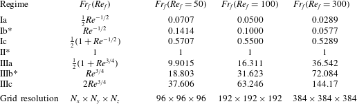
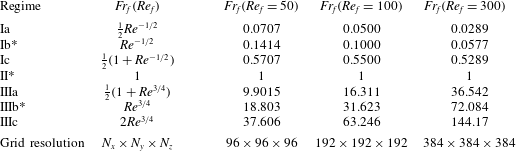
Values of
 $Fr_{f}$
as a function of
 $Re_{f}$
used in simulations of the NHQGE based on the seven regimes identified in figure 1. Domain size for each simulation is
 $10L_{f}\times 10L_{f}\times 1$
, where
 $L_{f}=1$
is the imposed forcing length scale. To ensure sufficient resolution we use the convention that
 ${\rm\Delta}x=2L_{K}$
, where
 $L_{K}=Re^{-3/4}$
is the dissipation length scale, giving the number of Fourier modes used in each Cartesian direction as
 $N_{x,y,z}=L_{b}Re^{3/4}/2$
. The Prandtl number is fixed at
 ${\it\sigma}=7$
for all simulations.
Fourier expansions are dealiased using the standard
 $2/3$
rule. To ensure sufficient resolution we use the convention that
 ${\rm\Delta}x=2L_{K}$
, where
 $L_{K}=Re^{-3/4}$
is the dissipation length scale for statistically steady flow. Use of this convention gives the number of Fourier modes used in each Cartesian direction as
 $N_{x,y,z}=L_{b}Re^{3/4}/2$
. Resolutions used in our numerical simulations are given in table 1.
The simulation parameters
 $(Re_{f},Fr_{f},{\it\sigma})$
are selected based on the regimes identified in figure 1. For a given
 $Re_{f}$
we vary
 $Fr_{f}$
so as to explore each of the seven regimes identified in figure 1. This process of selecting
 $Fr_{f}$
is outlined in table 1. All simulations are computed with
 ${\it\sigma}=7$
.
In addition to forcing vertical velocity we have also performed numerical simulations with buoyancy forcing as in Whitehead & Wingate (Reference Whitehead and Wingate2014); however, since the momentum equations decouple from the buoyancy equations for large
 $Fr_{f}$
, the injection of potential energy becomes unphysical. For this reason we only present results associated with the injection of vertical kinetic energy via the vertical velocity equation (3.9b
).
5 Results
The non-dimensional parameters defined in § 2 are based on a priori characteristic scales built from the energy injection rate
 ${\it\epsilon}_{f}$
and injection scale
 $L_{f}$
. These scales are not necessarily the same as the scales that truly characterize the flow; certainly it is not the case that the large-scale flows observed here occur on the forcing scale
 $L_{f}=1$
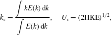
. For this reason we give a summary of a posteriori non-dimensional parameters that define the flows simulated. To do this we compute the centroid of energy spectra to get a characteristic wavenumber
 $k_{c}$
and associated length scale
 $L_{c}$
; we compute a characteristic velocity
 $U_{c}$
from the volume-averaged horizontal kinetic energy (HKE), that is,
 $$\begin{eqnarray}k_{c}=\frac{\displaystyle \int kE(k)\,\text{d}k}{\displaystyle \int E(k)\,\text{d}k},\quad U_{c}=(2\text{HKE})^{1/2},\end{eqnarray}$$
where
 $E(k)$
, for example, are the curves in figure 9. These non-dimensional measured values are then used to define a posteriori Reynolds and Froude numbers
 $$\begin{eqnarray}Re_{c}=\frac{U_{c}^{\ast }L_{c}^{\ast }}{{\it\nu}}=\frac{U_{f}^{\ast }U_{c}L_{f}^{\ast }L_{c}}{{\it\nu}}=Re_{f}U_{c}L_{c},\quad Fr_{c}=\frac{U_{c}^{\ast }}{N_{0}L_{c}^{\ast }}=\frac{U_{f}^{\ast }U_{c}}{N_{0}L_{f}^{\ast }L_{c}}=Fr_{f}\frac{U_{c}}{L_{c}}.\end{eqnarray}$$
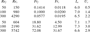
A posteriori
 $Fr_{c}$
and
 $Re_{c}$
values are summarized in table 2. Generally, characteristic horizontal scales are larger than
 $L_{f}$
, and characteristic velocities are larger than
 $U_{f}$
. This results in Reynolds numbers that are larger than
 $Re_{f}$
. The larger measured horizontal scale
 $L_{c}$
outweighs the increase in
 $U_{c}$
, leading to Froude numbers that are smaller, in some cases by an order of magnitude, than
 $Fr_{f}$
; however, what was considered weakly stratified as measured by
 $Fr_{f}$
remains so as measured by
 $Fr_{c}$
.
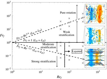
A qualitative partitioning of
 $(Re_{f},Fr_{f})$
-space using volume renders of vorticity. Values of
 $(Re_{f},Fr_{f})$
for which simulations were performed are denoted by an
 $\times$
(see table 1). The flow is characterized by layering, barotropization and an inverse cascade. For
 $Fr_{f}<1$
the flow organizes into well-defined layers (except at low-
 $Re_{f}$
, e.g.
 $Re_{f}=50$
) and when
 $Fr_{f}\geqslant 1$
layering is absent. We emphasize the presence of a dominant barotropic component of energy and a clear inverse cascade for all
 $Fr_{f}$
simulated. Similar flow characteristics are observed for buoyancy and vertical velocity (see figures 3 and 4).

Characteristic scales
 $U_{c}$
and
 $L_{c}$
computed from centroids of energy spectra and non-dimensional quantities
 $Re_{c}$
and
 $Fr_{c}$
based on the measured values
 $L_{c}$
and
 $U_{c}$
.
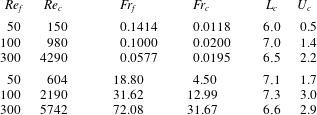
In performing DNS of the NHQGE (with the non-dimensional parameters outlined in table 1) two qualitatively identifiable regimes are observed. These regimes are associated with strong and weak stratification:
 $Fr_{f}<1$
and
 $Fr_{f}\geqslant 1$
, respectively. The regime diagram in figure 2 partitions
 $(Re_{f},Fr_{f})$
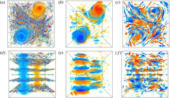
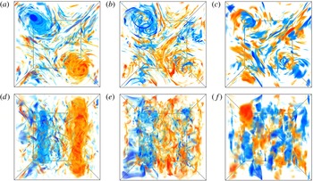
-space into these two regimes based on volume renders of vertical vorticity. In both regimes, the flow organizes into a large-scale, barotropic dipole with some additional small-scale turbulence. Figures 3 and 4 give renders for vertical vorticity, buoyancy and vertical velocity for strong and weak stratifications when
 $Re_{f}=300$
.
Volume renders of vertical vorticity
 ${\it\zeta}$
(a,d), buoyancy
 $b$
(b,e), and vertical velocity
 $w$
(c,f) for the case of strong stratification
 $Re_{f}=300,Fr_{f}=Re_{f}^{-1/2}$
. Top view (a–c), side view (d–f).

The strong-stratification regime (
 $Fr_{f}<1$
, figure 3) is distinguished by a tendency of the flow to form well-defined and sustained layers where small-scale turbulence is active and the local stratification is reduced. Layering is observed for
 $Re_{f}=100$
and
 $Re_{f}=300$
, but not for
 $Re_{f}=50$
. We conclude that the instability responsible for layering is inhibited by viscous effects at lower
 $Re_{f}$
. We note that layering, as observed in figure 3, is not observed for classical QG dynamics, where energy rapidly transfers to large vertical scales (Smith & Vallis Reference Smith and Vallis2001, Reference Smith and Vallis2002). In the second regime of weak stratification (
 $Fr_{f}\geqslant 1$
, figure 4) the columnar structures are unobstructed by layers, and evolve in a sea of small-scale turbulence.
Volume renders of vertical vorticity
 ${\it\zeta}$
(a,d), buoyancy
 $b$
(b,e), and vertical velocity
 $w$
(c,f) for the case of weak stratification
 $Re_{f}=300,Fr_{f}=Re_{f}^{3/4}$
. Top view (a–c), side view (d–f).

In both regimes, the energy accumulates primarily in the barotropic mode and at large horizontal scales, indicating a robust inverse cascade of energy. At lower Reynolds numbers
 $Re_{f}\leqslant 100$
(
 $Re_{c}$
up to
 ${\approx}2000$
), the total energy in the system reaches a statistical equilibrium. In addition to the inverse energy transfer, we diagnose a robust direct transfer of kinetic energy in the barotropic mode, which allows the small amount of energy injected by the baroclinic motions to be balanced by small-scale dissipation, leading to energy saturation. At higher Reynolds numbers,
 $Re_{f}=300$
(
 $Re_{c}$
greater than
 ${\approx}4000$
), the total energy shows no sign of saturation. These results are presented in more detail in the following subsections.
We note that these results do not necessarily represent universal properties of rotationally constrained stratified flow in every respect. Undoubtedly, the dynamic behaviour depends significantly on the method by which external energy is injected to excite motion. As mentioned above, the forcing method employed here excites vertical motion; therefore, it excites only wave modes and does not directly force the vortical mode. This approach to forcing aims to better understand the energetic pathway from three-dimensional baroclinic motions to two-dimensional barotropic motions.
5.1 Layering
Layering is observed in all fields, though most distinct in the renders of vertical vorticity shown in figure 3. To clarify terminology, we define layers to be the localized planar regions home to small-scale turbulence and occurring for
 $Fr_{f}<1$
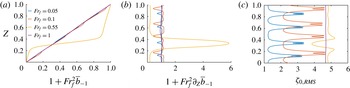
. Figure 5 shows the effect of strong stratification on the time-averaged vertical gradient of the total mean buoyancy profile and on the structure of
 ${\it\zeta}_{0,RMS}$
for simulations with
 $Re_{f}=100$
and
 $Fr_{f}\leqslant 1$
. Reduction of stratification within the layers is presumably associated with local turbulent mixing within the layers.
Time-averaged vertical profiles for
 $Re_{f}=100$
. Profiles of (a) total mean buoyancy, (b) vertical gradient of mean buoyancy and (c) RMS vertical vorticity. Layering occurs in horizontal planes where mean stratification is locally minimized. The effect on the stratification profile is due to the nature of vertical buoyancy flux. Similarly, layered structuring seen for vertical vorticity is due to vortex stretching. Layer locations coincide with locations of sharp local minima within the peaks of
 ${\it\zeta}_{0,RMS}$
. Layer height may be given by the distance between local maxima surrounding the singular local minima and indicate the presence of sublayers (jets). The vertical extent of layers and their sublayers is observed to increase with decreased stratification. Similar structuring is observed for vertical velocity, buoyancy, and dissipation.

Some basic characteristics of the location and height of layers are given by the mean buoyancy gradient and vertical profiles of
 ${\it\zeta}_{0,RMS}$
. The more informative of the two is the set of RMS profiles of vertical vorticity. The centre locations for layers coincide with the location of local minima within the peaks for
 ${\it\zeta}_{0,RMS}$
, and are obvious for
 $Fr_{f}=0.05$
and
 $Fr_{f}=0.1$
. The neighbouring local maxima may be used to give a reasonable metric for layer height, and indicate the presence of top and bottom sublayers that make up an entire layer. As stratification strength is decreased, layer height is observed to increase. This effect is illustrated in figure 5 as
 $Fr_{f}$
is increased from
 $0.05$
to
 $0.55$
. When
 $Fr_{f}=0.55$
there is only one large layer of reduced stratification and increased turbulence, and one smaller less-turbulent region of increased stratification that occupies approximately
 $Z\in [0.2,0.4]$
.
Finally, we note that the instantaneous dissipation rate for energy is increased within the layers. The instantaneous dissipation rate for horizontal kinetic energy is
 $Re_{f}^{-1}\overline{{\it\zeta}^{2}}^{\mathscr{A}}$
, and figure 5(c) clearly shows that this is increased within the layers. The dissipation rates for vertical kinetic energy and buoyancy variance are also locally increased within the layers (not shown). The dynamics leading to the formation of the layers is as yet unknown.
5.2 Time series, equilibration and average energy conversions
We find that total energy is largely dominated by horizontal kinetic energy and this becomes increasingly true as stratification weakens and the system approaches purely rotating dynamics. For this reason we focus primarily on the horizontal kinetic energy, hereafter HKE. However, before proceeding to discuss HKE we note that for all
 $Fr_{f}$
and
 $Re_{f}$
simulated the vertical kinetic energy takes on values close to
 $1/2$
(or
 $w_{0,RMS}=1$
). This behaviour of vertical kinetic energy is possibly due to the nature of our artificial forcing, where spatially correlated stochastic noise has unit amplitude (as results from setting
 ${\it\epsilon}_{f}=1$
). Additionally, the direct influence of this forcing precludes an unbiased measure of the natural tendency of, for example,
 $w_{0,RMS}$
as a function of
 $Fr_{f}$
.
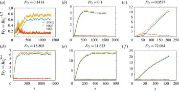
Time series of volume-averaged barotropic, baroclinic and total horizontal kinetic energy at
 $Fr_{f}=Re_{f}^{-1/2}$
(a–c) and
 $Fr_{f}=Re_{f}^{3/4}$
(d–f). These time series correspond to points where an
 $\times$
sits on the dashed lines in figure 2. A notable feature is the saturation of HKE at
 $Re_{f}=50$
and
 $Re_{f}=100$
. Computationally expensive simulations at
 $Re_{f}=300$
have not equilibrated. The barotropic component
 $\langle \text{HKE}\rangle$
contains nearly all the horizontal kinetic energy after an initial spin-up time. (a,d)
 $Re_{f}=50$
; (b,e)
 $Re_{f}=100$
; (c,f)
 $Re_{f}=300$
.

Figure 6 shows time series of volume-averaged HKE for strong stratification (
 $Fr_{f}=Re_{f}^{-1/2}$
, panels a–c) and weak stratification (
 $Fr_{f}=Re_{f}^{3/4}$
, panels d–f) at
 $Re_{f}=50,100$
and
 $300$
; the panels correspond to places where dashed lines in figure 2 intersect with a
 $\times$
. Each plot shows the volume-averaged barotropic, baroclinic and total horizontal kinetic energy, denoted as
 $\langle \text{HKE}\rangle$
,
 $\text{HKE}^{\prime }$
and HKE, respectively. In every case, the total HKE is dominated by the barotropic part; the only exception in our simulation suite being
 $Re_{f}=50$
and
 $Fr_{f}=0.0707$
, where the energy accumulates in a large vertical scale, but not barotropic (not shown). At lower Reynolds numbers,
 $Re_{f}\leqslant 100$
, the HKE saturates, while the simulations at
 $Re_{f}=300$
show no indication of saturation, and it is not clear whether it will eventually saturate.
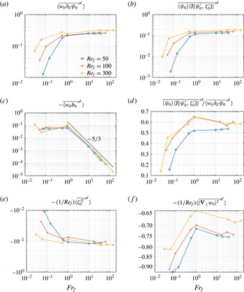
Equation (3.10) shows that vortex stretching and vertical buoyancy flux govern the conversion of VKE to HKE and PE to VKE, respectively. Furthermore, conversion of kinetic energy from the baroclinic component
 $\text{HKE}^{\prime }$
to the barotropic component
 $\langle \text{HKE}\rangle$
may be understood by multiplying inviscid equations (3.14a
) and (3.14b
) by
 $-\langle {\it\psi}_{0}\rangle$
and
 $-{\it\psi}_{0}^{\prime }$
to get
 $$\begin{eqnarray}\displaystyle & \displaystyle \partial _{t}\langle \text{HKE}\rangle :=\partial _{t}\left[{\textstyle \frac{1}{2}}\overline{|\boldsymbol{{\rm\nabla}}_{\bot }\langle {\it\psi}_{0}\rangle |^{2}}^{\mathscr{A}}\right]=\overline{\langle {\it\psi}_{0}\rangle \langle \text{J}[{\it\psi}_{0}^{\prime },{\it\zeta}_{0}^{\prime }]\rangle }^{\mathscr{A}}, & \displaystyle\end{eqnarray}$$
 $$\begin{eqnarray}\displaystyle & \displaystyle \partial _{t}\text{HKE}^{\prime }:=\partial _{t}\left[{\textstyle \frac{1}{2}}\langle \overline{|\boldsymbol{{\rm\nabla}}_{\bot }{\it\psi}_{0}^{\prime }|^{2}}^{\mathscr{A}}\rangle \right]=-\overline{\langle {\it\psi}_{0}\rangle \langle \text{J}[{\it\psi}_{0}^{\prime },{\it\zeta}_{0}^{\prime }]\rangle }^{\mathscr{A}}+\langle \overline{w_{0}^{\prime }\partial _{Z}{\it\psi}_{0}^{\prime }}^{\mathscr{A}}\rangle . & \displaystyle\end{eqnarray}$$
 $$\begin{eqnarray}\displaystyle \langle \text{HKE}_{dissip}\rangle & := & \displaystyle -\overline{\langle {\it\psi}_{0}\rangle \langle \text{J}[{\it\psi}_{0}^{\prime },{\it\zeta}_{0}^{\prime }]\rangle }^{\mathscr{A}}=-\frac{1}{Re_{f}}\overline{\langle {\it\zeta}_{0}\rangle ^{2},}^{\mathscr{A}}\end{eqnarray}$$
 $$\begin{eqnarray}\displaystyle \text{HKE}_{dissip}^{\prime } & := & \displaystyle \overline{\langle {\it\psi}_{0}\rangle \langle \text{J}[{\it\psi}_{0}^{\prime },{\it\zeta}_{0}^{\prime }]\rangle }^{\mathscr{A}}-\langle \overline{w_{0}^{\prime }\partial _{Z}{\it\psi}_{0}^{\prime }}^{\mathscr{A}}\rangle =-\frac{1}{Re_{f}}\langle \overline{{\it\zeta}_{0}^{\prime 2}}^{\mathscr{A}}\rangle ,\end{eqnarray}$$
 $$\begin{eqnarray}\displaystyle VKE_{dissip} & := & \displaystyle \langle \overline{w_{0}\partial _{Z}{\it\psi}_{0}}^{\mathscr{A}}\rangle -\langle \overline{w_{0}b_{0}}^{\mathscr{A}}\rangle -{\it\epsilon}_{f}=-\frac{1}{Re_{f}}\langle \overline{|\boldsymbol{{\rm\nabla}}_{\bot }w_{0}|^{2}}^{\mathscr{A}}\rangle ,\end{eqnarray}$$
 $$\begin{eqnarray}\displaystyle PE_{dissip} & := & \displaystyle \langle \overline{w_{0}b_{0}}^{\mathscr{A}}\rangle =-\frac{1}{Pe_{f}}\left\langle \frac{\overline{|\boldsymbol{{\rm\nabla}}_{\bot }b_{0}|^{2}}^{\mathscr{A}}}{\partial _{Z}\overline{b}_{-1}+Fr_{f}^{-2}S(Z)}\right\rangle .\end{eqnarray}$$
 ${\it\epsilon}_{f}$
at which energy is injected. Figure 7 shows volume and time-averaged energy conversion rates as functions of
 $Fr_{f}$
. These conversions are those given by (3.10) and (5.3). Additionally, for equilibrated flow, as is the case for simulations with
 $Re_{f}=50$
and
 $Re_{f}=100$
, energy conversion rates in figure 7 also provide the dissipation rates given by (5.4). In the following we compare and contrast the ways in which energy is converted from one type to another before being eventually dissipated in the two regimes.
Volume- and time-averaged energy fluxes and dissipation rates for
 $Re=50,100,300$
for strong (
 $Fr_{f}<1$
) and weak (
 $Fr_{f}\geqslant 1$
) stratification. Conversion of kinetic energy via (a) vortex stretching (appearing to be most efficient at
 $Fr_{f}\geqslant 1$
), (b) baroclinic forcing, and (c) vertical buoyancy flux (showing the decreased role of PE as
 $Fr_{f}$
increases above
 $Fr_{f}=1$
). Curves in (d) give the ratio of fluxes due to baroclinic forcing to that due to vortex stretching. Dissipation of
 $\text{HKE}^{\prime }$
and VKE are given in (e) and (f), respectively. For small values of
 $Fr_{f}$
approximately 90 % of all energy disappation is via VKE, while it accounts for approximately 75 % of energy dissipation at the weakest stratifications. For all simulations
 ${\it\epsilon}_{f}=1$
, and values here may be interpreted as the ratio of energy flux due to conversion or dissipation to energy injection due to forcing.

Before describing energy conversion we make note of figure 7(f), where it is clear that in both regimes most of the energy input to VKE is dissipated as VKE. A greater percentage of the total energy input is dissipated as VKE in the strong-stratification regime (more than 80 %), but a significant amount is still dissipated as VKE in the weak-stratification regime too (65 %–75 %). The vortical mode lacks vertical velocity, and the fact that most of the energy injected to wave modes does not convert to horizontal kinetic or potential energy is an indication of the weakness of the wave–vortex interactions in the rapidly rotating regime.
Figure 7(a) shows the mean energy conversion rate from VKE to HKE by vortex stretching. In the weakly stratified regime, the percentage of total energy injection that is converted to HKE remains approximately 20 %, with a very weak sensitivity to the Reynolds and Froude numbers. By contrast, as the stratification increases past
 $Fr_{f}\approx 1$
, the rate of conversion to HKE drops rapidly, with less conversion for lower Reynolds numbers. Indeed, of the total input, only approximately 3 %–4 % is converted to HKE at the smallest Froude number at
 $Re_{f}=100$
. This is consistent with known results for the strongly stratified, rapidly rotating quasi-geostrophic regime, where wave modes interact extremely weakly with vortical modes.
We next examine conversion of baroclinic to barotropic HKE. From (3.14) it is clear that baroclinic motions are solely responsible for exciting barotropic motions. In both regimes of weak and strong stratification, we find that the conversion of baroclinic to barotropic energy (
 $F=\overline{\langle {\it\psi}_{0}\rangle \langle \text{J}[{\it\psi}_{0}^{\prime },{\it\zeta}_{0}^{\prime }]\rangle }^{\mathscr{A}}$
) is roughly statistically steady in time and positive. Time-averaged values for the conversion
 $F$
are summarized in figure 7(b). Like the rate of conversion from VKE to HKE, the rate of conversion from baroclinic to barotropic HKE is insensitive to
 $Re_{f}$
and
 $Fr_{f}$
in the weakly stratified regime, and drops sharply with
 $Fr_{f}$
in the strongly stratified regime. Not only does the gross rate of energy injection to the barotropic mode decrease with
 $Fr_{f}$
in the strongly stratified regime, the percentage of conversion from VKE to HKE that further converts to barotropic HKE decreases too, as shown by figure 7(d). For example, at the smallest Froude number and at
 $Re_{f}=100$
, less than 40 % of the conversion to HKE further converts to barotropic HKE. As mentioned above, the simulation with
 $Re_{f}=50$
at the strongest stratification does not exhibit barotropization, which may be due to an insufficient
 $O(10^{-3})$
energy flux into the barotropic mode compared to viscous dissipation (see figure 7
b and e).
This result, that the rate of energy injection to the barotropic mode decreases with the Froude number, seems to contradict the results of Marino et al. (Reference Marino, Mininni, Rosenberg and Pouquet2013), who found that the transfer of energy to the barotropic mode is more efficient at small Froude numbers than at large Froude numbers. The difference is that we are examining the rate of energy injection to the barotropic mode as compared to the rate of total energy injection (figure 7 b) and as compared to the rate of HKE forcing (figure 7 d), while they examined a time scale defined as an energy divided by the rate of energy injection to the barotropic mode. Figure 6, especially panels (b,e), shows that the net barotropic energy is larger at large Froude number than at small Froude number for a given forcing and Reynolds number; together with the results in figure 7, this suggests that it may be more accurate to say that energy transfer to the barotropic mode is more efficient at large Froude numbers than at small ones.
Clearly, the saturation of the barotropic energy observed at moderate Reynolds numbers is not the result of a shutdown of injection to the barotropic mode. The fact that the barotropic energy saturates despite a net positive energy injection indicates that there must be a net dissipation to balance the forcing. None of our simulations use a large-scale dissipation, so the barotropic dissipation must be viscous. In § 5.3 we diagnose a small yet robust direct cascade of barotropic kinetic energy that carries enough energy to small-scale dissipation that the total barotropic energy is able to equilibrate at
 $Re_{f}\leqslant 100$
. Since the rate of injection matches the rate of dissipation at equilibrium, the results in figure 7(b) are equivalent to the barotropic dissipation rate (at least for
 $Re_{f}\leqslant 100$
, where the energy saturates). We therefore infer that the barotropic dissipation rate, which is equivalent to the strength of the forward cascade in the barotropic mode, increases as the Reynolds number increases for
 $Fr_{f}\leqslant 1$
, and remains approximately constant for
 $Fr_{f}\geqslant 1$
.
Energy injected directly to VKE also converts to potential energy; the mean rate of conversion from VKE to PE is shown in figure 7(c). This conversion out of VKE displays somewhat opposite behaviour to the conversion from VKE to HKE: in the strongly stratified regime the conversion remains flat, insensitive to both Reynolds and Froude numbers, while in the weakly stratified regime the conversion decreases rapidly as the stratification weakens, and with little dependence on Reynolds number. A priori, one expects conversion from VKE to PE to diminish as Froude numbers increase, since PE becomes negligible in the pure-rotation limit.
To summarize, in both regimes, energy injected to VKE is primarily dissipated as VKE, and there is a net positive conversion to barotropic KE that is, for moderate Reynolds numbers, balanced by dissipation leading to total energy equilibration. In the strongly stratified regime the conversion to baroclinic HKE decreases with
 $Fr_{f}$
, as does the rate of conversion to barotropic HKE, while the rate of conversion to PE remains moderate and insensitive to
 $Fr_{f}$
. In the weakly stratified regime the conversion to baroclinic HKE remains moderate and insensitive to
 $Fr_{f}$
, as does the rate of conversion to barotropic HKE, while the rate of conversion to PE decreases rapidly as
 $Fr_{f}$
increases.
5.3 Cospectra and scales active in energy conversion
While illuminating, the discussion in § 5.2 is based on global scalars obtained from volume and time averages, and is altogether lacking any spatial information. To improve on this, vertically and time-averaged cospectra are computed. These one-dimensional cospectra are calculated by decomposing horizontal means of pointwise physical space products as the sum of Fourier space products, reordering sums over circular rings, binning, and averaging in the
 $\hat{\boldsymbol{z}}$
direction, i.e.,
 $$\begin{eqnarray}(f,g)(\widetilde{k}_{\bot })=\left\langle \mathop{\sum }_{0<|\widetilde{k}_{\bot }^{\prime }-\widetilde{k}_{\bot }|\leqslant 1}\overline{\hat{f}}(k_{\bot }^{\prime },Z){\hat{g}}(k_{\bot }^{\prime },Z)\right\rangle ,\quad \widetilde{k}_{\bot }=\frac{k_{\bot }}{k_{0}}=1,2,3,\ldots ,\end{eqnarray}$$
where
 $\widetilde{k}_{\bot }$
and
 $\widetilde{k}_{\bot }^{\prime }$
are horizontal wavenumbers normalized by the box scale
 $k_{0}=2{\rm\pi}/10$
; the bar here denotes complex conjugation, hats denote horizontal Fourier amplitudes, and angle brackets denote a vertical average. Furthermore, the temporal mean of cospectra are computed to provide the scales active in energy conversion on average. This rescaling of the wavenumbers is convenient, since it leads to integer wavenumbers; for example, the scaled forcing wavenumber is
 $\widetilde{k}_{\bot }=10$
, while the unscaled version is
 $k_{\bot }=2{\rm\pi}$
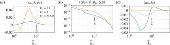
. Figure 8 shows cospectra of vortex stretching, barotropization of HKE, and vertical buoyancy flux for simulations with
 $Re_{f}=100$
and with
 $Fr_{f}=Re_{f}^{-1/2},1,Re_{f}^{3/4}$
. Similar cospectra are observed for
 $Re_{f}=50$
and
 $Re_{f}=300$
. Although simulations with
 $Re_{f}=300$
have not reached a dynamic equilibrium, they too convey the trends observed for
 $Re_{f}=100$
in figure 8.
Vertically and time-averaged horizontal cospectra of energy fluxes at
 $Re_{f}=100$
for times proceeding energy saturation. Cospectra in (a) give conversions between HKE and VKE by vortex stretching. Cospectra in (b) give the barotropization of HKE and indicate a flux of
 $\text{HKE}^{\prime }$
into the gravest horizontal mode at
 $\widetilde{k}_{\bot }=1$
. Cospectra in (c) give conversions between VKE and PE by vertical buoyancy flux and strongly indicate that these conversion become increasingly weak as
 $Fr_{f}$
increases beyond unity.

For the strongest stratification, figure 8(a) indicates that conversion to
 $\text{HKE}^{\prime }$
by vortex stretching occurs at all available scales, with a preference for
 $\widetilde{k}_{\bot }\approx 5$
(or
 $L\approx 2L_{f}$
), and may hint at a preferred scale for wave–vortex interactions. The centroid (or the average wavenumber) active for this energy conversion by vortex stretching is just less than
 $\widetilde{k}_{f}=10$
(or
 $L\approx L_{f}=1$
); however, the efficiency of vortex stretching is best at
 $L=2L_{f}$
. The barotropization of HKE in figure 8(b) shows that horizontal baroclinic motions act to force barotropic motions at all scales; however, with a strong preference for the largest available horizontal scale. That this baroclinic forcing is, on average, positive definite is consistent with (5.4a
) and implies that this barotropized energy is trapped in the barotropic mode until it is viscously dissipated. Figure 8(c) shows that the conversion between PE and VKE depends on scale: VKE is converted to PE for
 $\widetilde{k}_{\bot }<\widetilde{k}_{f}$
, and PE is converted back to VKE for
 $\widetilde{k}_{\bot }\gtrsim \widetilde{k}_{f}$
, with a net conversion to PE and a peak efficiency at
 $\widetilde{k}_{\bot }=3\;(L\approx 3.3L_{f})$
.
When stratification weakens and
 $Fr_{f}=1$
, there is still a net conversion from VKE to HKE by vortex stretching. However, stretching now converts HKE back to VKE at the two largest available scales
 $(\widetilde{k}_{\bot }=1,2)$
. Vortex stretching continues to most efficiently convert vertical to horizontal kinetic energy at
 $\widetilde{k}_{\bot }=5$
(
 $L=2L_{f}$
, the peak in figure 8
a), and is nearly four times the conversion seen at stronger stratification. Baroclinic motions continue to drive barotropic motions in a fashion similar to that at stronger stratification; however, this is done with slightly increased efficiency, especially for
 $5<\widetilde{k}_{\bot }<20$
(figure 8
b). Potential energy becomes weak to the point were the feedback to vertical kinetic energy for
 $\widetilde{k}_{\bot }>\widetilde{k}_{f}$
is substantially reduced and a preference to convert vertical to potential energy at scales
 $\widetilde{k}_{\bot }=5\;(L=2L_{f})$
is smaller than that at
 $Fr_{f}=Re_{f}^{-1/2}$
.
Finally, for the weakest stratification, where
 $Fr_{f}=Re^{3/4}$
, conversion from VKE to HKE is very similar to
 $Fr_{f}=1$
, with the exception that conversion back to vertical kinetic energy only occurs at
 $\tilde{k}_{\bot }=2$
rather than both
 $\tilde{k}_{\bot }=1$
and
 $2$
. At all other scales vortex stretching acts to move energy from vertical motions to baroclinic horizontal motions, and does so most efficiently near
 $\tilde{k}_{\bot }=5$
(the peak in figure 8
a). That the largest scale now plays a role via vortex stretching in converting vertical to horizontal energy (contrary to what occurs when
 $Fr_{f}=1$
) might be explained by an increased pool of energy made available by the decreased role of buoyancy (see figure 7
c). Barotropization of horizontal kinetic energy, forced by baroclinic motions, is virtually identical to
 $Fr_{f}=1$
, and figure 8(c) iterates the insignificance of buoyancy and an approach to purely rotating dynamics.
Figure 8(b) indicates that energy input to the barotropic mode occurs primarily at the largest scale at all Froude numbers. Similar behaviour was observed by Larichev & Held (Reference Larichev and Held1995) in simulations of two-layer quasi-geostrophic turbulence.
5.4 Energy spectra
Vertically and time-averaged horizontal energy spectra for simulations with
 $Re_{f}=300$
,
 $Fr_{f}=0.0577$
and
 $Fr_{f}=72.084$
are computed using (5.5) and are given in figure 9. Similar spectra are observed for remaining values of
 $Fr_{f}$
and at lower
 $Re_{f}$
. Both plots give barotropic,
 $\langle \text{HKE}\rangle =(-\langle {\it\psi}_{0}\rangle ,\langle {\it\zeta}_{0}\rangle )$
, and baroclinic,
 $\text{HKE}^{\prime }=(-{\it\psi}_{0}^{\prime },{\it\zeta}_{0}^{\prime })$
, components of the total horizontal kinetic energy spectrum,
 $\text{HKE}=(-{\it\psi}_{0},{\it\zeta}_{0})$
.
Vertically and temporally averaged horizontal energy spectra for
 $Re_{f}=300$
with (a)
 $Fr_{f}=0.0577$
and (b)
 $Fr_{f}=72.084$
. Each figure shows the barotropic,
 $\langle \text{HKE}\rangle =(-\langle {\it\psi}_{0}\rangle ,\langle {\it\zeta}_{0}\rangle )$
, and baroclinic,
 $\text{HKE}^{\prime }=(-{\it\psi}_{0}^{\prime },{\it\zeta}_{0}^{\prime })$
, components of horizontal kinetic energy spectra,
 $\text{HKE}=(-{\it\psi}_{0},{\it\zeta}_{0})$
. A
 $k_{\bot }^{-3}$
energy spectra at small wavenumber is due to energy-containing scales in the barotropic subspace for both strong and weak stratification. For strong stratification and larger wavenumber, a steep
 $k_{\bot }^{-20/3}$
scaling for barotropic energy gives way to a
 $k_{\bot }^{-3}$
scaling near the dissipation range. For weak stratification, the steep scaling is short-lived.

For both strong and weak stratification, a
 $\widetilde{k}_{\bot }^{-3}$
energy spectrum for
 $\widetilde{k}_{\bot }\in [1,3]$
is dominated by barotropic energy. For strong stratification, the barotropic energy drops off steeply as
 $\widetilde{k}_{\bot }^{-20/3}$
for
 $k_{\bot }\in [3,8]$
, and gives way to a
 $\widetilde{k}_{\bot }^{-3}$
scaling below the forcing scale. At weak stratification, the steep scaling is short-lived and the barotropic spectrum quickly gives way to a
 $\widetilde{k}_{\bot }^{-3}$
scaling near the forcing scale. The presence (absence) of the steep drop-off in energy for strong (weak) stratification might be explained, to some extent, by the weaker (stronger) baroclinic forcing for
 $\widetilde{k}_{\bot }\in [3,8]$
(see figure 8
b); indeed, the shape of the forcing cospectrum decreases (sustains) in this range. In turn, the difference in behaviour of baroclinic forcing might be explained by flow morphology. At strong stratification, horizontal layers appear and are associated with increased viscous effects that may disrupt collinearity of baroclinic advection of the baroclinic vorticity with the barotropic streamfunction (figure 8
b). When layers are absent at weaker stratification, so are associated regions of increased viscous effects, and the result is an increased efficiency of baroclinic forcing (figure 8
b).
For strong stratification, as
 $\widetilde{k}_{\bot }\!$
increases and barotropic energy becomes subdominant, the baroclinic energy spectra scales as
 $\widetilde{k}_{\bot }^{-5/3}$
for
 $\widetilde{k}_{\bot }\in [4,\approx 20]$
. When stratification is weaker, this scaling range appears to narrow, which may be explained by increased vortex stretching, which acts to force baroclinic energy most efficiently in the range
 $\widetilde{k}_{\bot }\in [4,5]$
.
Energy transfer map showing how barotropic triad interactions move energy within the barotropic subspace for equilibrated dynamics where
 $Re_{f}=100$
and
 $Fr_{f}=0.1$
. The colourmap
 $T_{\widetilde{k}_{\bot }\widetilde{p}_{\bot }}$
shows how energy at wavenumber
 $\widetilde{k}_{\bot }$
is gained or lost due to interaction with wavenumber
 $\widetilde{p}_{\bot }$
, where red (blue) denotes a gain (loss) of energy. The vertical profile (on the right) is the result of summing the transfer map
 $T_{\widetilde{k}_{\bot }\widetilde{p}_{\bot }}$
over
 $\widetilde{p}_{\bot }$
to get
 $T_{\widetilde{k}_{\bot }}$
. Note the scale for
 $T_{\widetilde{k}_{\bot }}$
is
 $O(10^{-5})$
, an indication that energy transfer via triad interaction is weak relative to baroclinic forcing. Similar results are seen for weak stratification. Red (blue) shading indicates that energy is transferred into (out of) wavenumber
 $\widetilde{k}_{\bot }$
through interactions with wavenumber
 $\widetilde{p}_{\bot }$
.

5.5 Barotropization and inverse cascade
It is interesting to consider the barotropic dynamics, since these motions are governed by the two-dimensional vorticity equation (3.14a
). If two-dimensional dissipative flow is forced at scales well separated from frictional effects acting on energy and enstrophy then an upscale energy range and a downscale enstrophy range form where, in the limit of vanishing viscosity, the downscale transfer of energy through the enstrophy range is expected to vanish. In our simulations, only a fraction of the energy converted to baroclinic HKE by vortex stretching goes on to force the barotropic vorticity equation (this fraction depends on
 $Fr_{f}$
; see figure 7
d). Figure 8(b) illustrates that baroclinic motions establish a natural injection of energy directly into the gravest barotropic mode, so that the accumulation of energy at large scales in the barotropic mode does not result primarily from a two-dimensional inverse-cascade process. Dissipation in the barotropic subspace, therefore, occurs through a non-zero forward energy cascade. Figure 10 gives a detailed map of the transfer of energy between barotropic Fourier modes performed by barotropic triad interactions for equilibrated flow at
 $Re_{f}=100$
(for details see Rubio et al. (Reference Rubio, Julien, Knobloch and Weiss2014)). The colourmap
 $T_{\widetilde{k}_{\bot }\widetilde{p}_{\bot }}$
shows how energy at wavenumber
 $\widetilde{k}_{\bot }$
is gained or lost due to interaction with wavenumber
 $\widetilde{p}_{\bot }$
, where red (blue) denotes a gain (loss) of energy. The near-diagonal elements of this map at large wavenumber show a local forward transfer of energy to small scales coexisting with a non-local inverse cascade at larger scales. The accumulation of energy at large horizontal scales in the barotropic mode in these rapidly rotating flows is primarily the result of three-dimensional baroclinic motions interacting to directly induce large-scale and vertically invariant structures; it is not primarily a result of baroclinic injection to an intermediate scale, followed by a purely barotropic inverse cascade to larger scales.
6 Conclusions
We have presented an investigation into stably stratified and rapidly rotating turbulence using the asymptotically reduced NHQGE set valid for
 $Ro\ll 1$
describing geostrophically balanced flow. Such a regime may be relevant to abyssal oceans (where observations indicate the presence of weak stratification), as well as planetary and stellar interiors (in regions where stratification transitions from unstable to stable). Within this parameter regime the Proudman–Taylor constraint is relaxed/broken by allowing anisotropic dynamics with vertical scales
 $O(Ro^{-1})$
larger than horizontal scales. In this setting, slow inertia-gravity waves with order-one frequencies are retained and not filtered; moreover, time scales for nonlinear eddy dynamics and anisotropic inertia-gravity waves are not asymptotically separated (see § 2.1). Numerical simulations with wave–eddy interactions are performed where motions are induced by a stochastic injection of vertical kinetic energy; doing so only provides wave energy, and any emergence of vortical mode energy must originate from wave–eddy interactions (see § 4).
Our results reveal two regimes: corresponding to strong (
 $Fr_{f}<1$
) and weak (
 $Fr_{f}\geqslant 1$
) stratification. These regimes are primarily distinguished by the presence at strong stratification of thin horizontal turbulent layers in which energy transfer and dissipation are most active. As
 $Fr_{f}$
increases up to unity, layer thickness also increases until the layers occupy the entire vertical extent of the domain. We note such layer formation, as defined in § 5.1, is not observed for classical QG dynamics, for which inertia-gravity waves are entirely absent. Evidence of layering has been previously observed in experiments of decaying purely stratified turbulence (Billant & Chomaz Reference Billant and Chomaz2000) and numerical studies of decaying rotating-stratified turbulence (Cambon Reference Cambon2001), but not in previous studies of rapidly rotating, strongly stratified, forced-dissipative turbulence. Unlike the ‘pancake’ structures that form in stratified turbulence (Kimura & Herring Reference Kimura and Herring2012), the layers here are localized and long-lived. Also, vertical shear of the horizontal velocity
 $\partial _{z}u_{\bot }$
is absent from the reduced equations governing the dynamics, so layer formation cannot be associated with shear instabilities such as Kelvin–Helmholtz or symmetric instability. Unlike the ‘staircase’ layering in doubly diffusive convection (Stellmach et al.
Reference Stellmach, Traxler, Garaud, Brummell and Radko2011) and stratified turbulence, (Phillips Reference Phillips1972; Balmforth, Smith & Young Reference Balmforth, Smith and Young1998) the layers consist of thin regions of reduced stratification. Similarly, the potential-vorticity staircase structures associated with large-scale zonal jets (Dritschel & McIntyre Reference Dritschel and McIntyre2008) are associated with thin regions of large potential-vorticity gradients, rather than thin regions with reduced gradients. We conjecture that the existence of our layers is related to our use of vertical velocity forcing, in the sense that other kinds of forcing may disrupt the dynamics leading to layer formation. Here, layer formation at
 $Fr_{f}<1$
is associated with mixing by vertical buoyancy flux and energy conversion by vortex stretching (evident in vertical profiles in figure 5). Additionally, vertical profiles of stratification and RMS vertical vorticity quantify layer location and thickness.
In addition to the presence or absence of layers, the regimes are distinguished by energetics. In the strongly stratified regime only a small percentage of the energy injection rate to vertical kinetic energy is converted to horizontal kinetic energy, and a modest amount is converted to potential energy. In the weakly stratified regime only a small percentage of the energy injection rate to vertical kinetic energy is converted to potential energy, and a modest amount is converted to horizontal kinetic energy.
Both regimes are characterized by the emergence of a large-scale barotropic dipole (see figure 2). When the Reynolds number is not too large (
 $Re_{f}\leqslant 100$
, or
 $Re_{c}\leqslant 2000$
) the system energy reaches a statistically steady state, evidence that geostrophically balanced flow is capable of establishing a direct route to dissipation. The process leading to energy saturation is attributed to a downscale transfer of kinetic energy within the barotropic mode, which balances the injection of barotropic energy by baroclinic motions. Although the net energy can become quite large, in all cases the reduced equations guarantee that the rotational constraint is not lost: the forward cascade does not result from a loss of rotational constraint. Similarly, in the small-Froude-number regime, the bulk a posteriori Froude numbers remain small so that the dynamics remain strongly influenced by stratification. It may be the case that the strong-stratification constraint is lost within the layers, but these are clearly not barotropic and cannot directly explain the barotropic forward cascade. At the largest Reynolds number considered here (
 $Re_{f}=300$
,
 $Re_{c}\geqslant 4000$
), the energy did not saturate, and it was not clear whether it would have saturated in a longer simulation. In an oceanographic setting, viscous boundary layers can act to remove large-scale barotropic energy, which could lead to energy saturation even in high-energy cases where the forward cascade might not suffice.
Another distinct trait of the flows studied here is that three-dimensional baroclinic motions interact in such a way as to inject energy into the largest barotropic scales; therefore, the accumulation of energy at the largest scales in the barotropic mode is not the result of an upscale transfer within the barotropic mode.
Acknowledgements
The authors would like to thank P. Bartello and M.-L. Timmermans for helpful discussions. This work was supported by the National Science Foundation under grants EAR CSEDI no. 1067944 and DMS no. 1317666 (K.J.), DMS no. 1444503 (D.N.), and in part by NSF-OCE 1245944 (J.B.W.). This work utilized the Janus supercomputer, which is supported by the National Science Foundation (award number CNS-0821794) and the University of Colorado Boulder. The Janus supercomputer is a joint effort of the University of Colorado Boulder, the University of Colorado Denver and the National Center for Atmospheric Research.