1 Introduction
The dynamics of ice sheets and glaciers depend sensitively on their thermal structure. Many ice masses are polythermal, containing both cold ice, with temperature below the melting point, and temperate ice, with temperature at the melting point. The temperate ‘ice’ is really an ice–water mixture, with water being produced at grain boundaries by dissipative heating. Although the water content is typically small, it can have an important effect. As well as altering the thermodynamics, water content controls ice viscosity and hence deformation, and internal melting and percolation affect mass balance and hydrology.
This paper concerns the theory required to model an ice mass’s polythermal structure. The essential demands of such a theory are to determine the temperature of the cold ice and the water content of the temperate ice, and at the same time to determine which regions are in fact cold and which temperate. In this sense, the problem is a free-boundary problem. Various models already exist, but our focus here will be specifically on the treatment of the temperate ice, which is different from existing models. In particular, we explicitly model the drainage of water driven by gravity and pressure gradients. Our aim is for a model that consistently describes this process, but that is nevertheless simple enough to be incorporated in operational ice sheet simulations.
Extensive discussions on the theory for polythermal ice are provided by Fowler & Larson (Reference Fowler and Larson1978), Hutter (Reference Hutter1982) and Fowler (Reference Fowler1984). At the most basic level, the fundamental ingredient is energy conservation, which manifests itself as an equation for temperature in the cold ice and an equation for porosity, i.e. moisture content, in the temperate ice. The theories differ primarily in their treatment of moisture transport (and associated latent heat transport), and in their treatment of cold–temperate boundaries.
The simplest assumption to make is that moisture is simply advected with the ice. Alternatively, moisture transport relative to the ice can be described either with a diffusive flux proportional to the gradient of porosity, or with a Darcy flux proportional to the permeability and potential gradient. Most current models adopt the diffusive flux (Aschwanden & Blatter Reference Aschwanden and Blatter2009; Aschwanden et al.
Reference Aschwanden, Bueler, Khroulev and Blatter2012), which is typically assumed to be small. Because this approach does not allow for drainage under gravity, it tends to cause a build-up of moisture, so that large porosities (greater than
 $1\,\%$
, say) can occur. Some form of cap on the porosity and instantaneous drainage to the bed is often adopted to deal with this (e.g. Greve Reference Greve1997b
; Aschwanden et al.
Reference Aschwanden, Bueler, Khroulev and Blatter2012), but a more realistic description of how gravity-driven drainage removes moisture from the ice is desirable.
Here we present a model for polythermal ice built on the theory for the viscous compaction of partially molten polycrystalline solids, similar to models used for viscous compaction in the partially molten mantle (Turcotte & Ahern Reference Turcotte and Ahern1978; McKenzie Reference McKenzie1984). The model accounts for conservation of energy throughout the ice mass by tracking changes in specific and latent heat content in the ice mass, solving the standard heat equation in the ‘cold’ parts of the domain and a coupled model for melt water drainage and viscous compaction (which determines the water pressures that partially drive the flow of melt through the porous ice matrix) in the temperate part of the domain.
The main advantage of our model over existing approaches used in ice sheet simulations is that we are able to incorporate gravity- and pressure-gradient-driven drainage of melt water in the temperate regions in a self-consistent way as determined by Darcy’s law, while also determining the location for the cold–temperate boundary as a free boundary in a way that accounts for phase changes that occur there.
In practice, the application of polythermal models is often intricately tied up with the numerical method used to solve the problem. Early numerical calculations (Blatter & Hutter Reference Blatter and Hutter1991; Greve Reference Greve1997a ) solved equations for the cold and temperate ice separately, applying jump conditions to calculate explicitly where the cold–temperate transition should occur. More recently, the favoured approach has been to solve an equation for the energy throughout the whole domain, and then to infer from that what the temperature and moisture content are. Provided an appropriate numerical scheme is used, the free-boundary location should be automatic. This approach is commonly referred to as an enthalpy method. It is used in other multiphase problems such as alloy solidification and magma dynamics, and its use in glaciology in the form of an enthalpy-gradient method (where moisture flux is diffusive) is described by Aschwanden & Blatter (Reference Aschwanden and Blatter2009) and more extensively by Aschwanden et al. (Reference Aschwanden, Bueler, Khroulev and Blatter2012). In this paper, we show how this existing framework can be extended to describe gravity- and pressure-gradient-driven moisture transport, without having to assume that moisture flux is diffusive.
We test an enthalpy-based finite volume method for the full, time-dependent version of our polythermal ice model against a direct solution of one-dimensional steady states by a multiple shooting method. By showing close agreement between the two, we establish our finite volume discretization as a computationally viable method. In addition, we use these solutions to investigate the generic behaviour of the model. We focus on competing mechanisms for melt water transport through advection, gravity-driven drainage and drainage caused by englacial water pressure gradients, and on the difference between cold–temperate boundaries at which ice flows into and out of the temperate domain. Thirdly, we compare these numerical solutions against an asymptotic solution in the limit of small compaction pressure gradients, where transport of moisture is dominated by advection and gravity-driven drainage. Lastly, we use this asymptotic solution to motivate a simple modification of existing enthalpy gradient models that can emulate the behaviour of our more complete model in the relevant small pressure-gradient limit.
The layout of this paper is as follows. We begin in § 2 with the basic theory. After summarizing the standard equations for cold ice, we describe the equivalent expressions for mass and energy conservation within temperate ice. Darcy’s law and the concept of the compaction pressure are introduced, as well as the jump conditions to apply at cold–temperate boundaries. The model is then non-dimensionalized and approximated to arrive at a reduced model. The approximations amount to ignoring the density change upon melting and freezing, and ignoring the effect of internal melting on ice mass balance. Both of these approximations are effectively implicit in existing models, and they allow us to retain the incompressibility constraint for the temperate ice. The reduced model is summarized in § 2.5.
In § 3 we discuss the different boundary conditions that apply. These are somewhat delicate, depending on whether the ice near the boundary is cold or temperate, and on the direction of ice flow. Next, we formulate a one-dimensional steady version of the model complete with the relevant boundary conditions in § 4. Numerically computed results are presented in § 5 and we conclude with a discussion in § 6, where we also present an enhanced enthalpy-gradient model that accounts for gravity-driven drainage. Many of the technical aspects of our work are relegated to the appendices, where we sketch our numerical methods and some of the technical aspects associated with the asymptotic solution, a basic version of which is stated in § 4. Extensive additional detail on numerical and asymptotic methods can be found in the supplementary material available at http://dx.doi.org/10.1017/jfm.2016.251.
2 Model
2.1 Cold ice
The standard model to describe ice sheet flow is that of an incompressible power-law viscous fluid, governed by equations of mass and force balance,
 $$\begin{eqnarray}\displaystyle & \displaystyle \boldsymbol{{\rm\nabla}}\boldsymbol{\cdot }\boldsymbol{u}, & \displaystyle\end{eqnarray}$$
 $$\begin{eqnarray}\displaystyle & \displaystyle \frac{\partial {\it\tau}_{ij}}{\partial x_{j}}-\frac{\partial p}{\partial x_{i}}=-{\it\rho}g_{i}, & \displaystyle\end{eqnarray}$$
 $$\begin{eqnarray}\displaystyle {\it\tau}_{ij}=A^{-1/n}D^{1/n-1}\unicode[STIX]{x1D60B}_{ij},\quad \unicode[STIX]{x1D60B}_{ij}=\frac{1}{2}\left(\frac{\partial u_{i}}{\partial u_{j}}+\frac{\partial u_{j}}{\partial x_{i}}\right),\quad D=\sqrt{\unicode[STIX]{x1D60B}_{ij}\unicode[STIX]{x1D60B}_{ij}/2}, & & \displaystyle\end{eqnarray}$$
where repeated indices are summed over. Here,
 $\boldsymbol{u}=(u_{1},u_{2},u_{3})$
is the velocity vector,
 $\unicode[STIX]{x1D60B}_{ij}$
is the strain rate tensor,
 $D$
is its second invariant,
 ${\it\tau}_{ij}$
is the deviatoric stress tensor,
 $p$
is the pressure,
 ${\it\rho}$
is the density of ice and
 $\boldsymbol{g}=(g_{1},g_{2},g_{3})$
is the acceleration due to gravity.
 $A$
and
 $n$
are coefficients in the flow law. Temperature enters the problem because the coefficient
 $A$
depends strongly on temperature, usually with an assumed Arrhenius dependence. Thus, the model is coupled to an energy equation,
 $$\begin{eqnarray}\displaystyle & \displaystyle {\it\rho}c\left(\frac{\partial T}{\partial t}+\boldsymbol{u}\boldsymbol{\cdot }\boldsymbol{{\rm\nabla}}T\right)-\boldsymbol{{\rm\nabla}}\boldsymbol{\cdot }\left(K\boldsymbol{{\rm\nabla}}T\right)=a, & \displaystyle\end{eqnarray}$$
 $$\begin{eqnarray}\displaystyle & \displaystyle a={\it\tau}_{ij}\unicode[STIX]{x1D60B}_{ij}, & \displaystyle\end{eqnarray}$$
in which
 $c$
is the specific heat capacity,
 $K$
is the thermal conductivity and
 $a$
is the viscous dissipation.
2.2 Temperate ice
When ice reaches the melting point
 $T_{m}$
, there are three potentially important changes required to this model. Firstly, the temperate ice is porous, and with a non-zero porosity
 ${\it\phi}$
(volume fraction), the flow-law coefficient may depend on porosity as well as temperature
 $A=A(T,{\it\phi})$
(Duval Reference Duval1977; Lliboutry & Duval Reference Lliboutry and Duval1985). Secondly, the energy balance must be altered to account for the latent heat required to melt or refreeze the interstitial water (and hence determine the evolution of the porosity). Thirdly, the porous ice matrix may be permeable, and the ability for water to drain means that the ice–water mixture is no longer necessarily incompressible.
To address these changes, we consider the general mixture form of the mass, momentum and energy conservation equations for permeable temperate ice, broadly working by analogy with models for melt extraction from the Earth’s mantle (e.g. Hewitt & Fowler Reference Hewitt and Fowler2008). The ice is assumed to have porosity
 ${\it\phi}$
, and we denote the internal melting rate (the rate of mass conversion from ice to water) by
 $m$
. In terms of the average pore-water velocity
 $\boldsymbol{u}_{w}$
we also define the relative moisture flux (or Darcy transport velocity)
 $$\begin{eqnarray}\displaystyle \boldsymbol{j}\equiv {\it\phi}(\boldsymbol{u}_{w}-\boldsymbol{u}), & & \displaystyle\end{eqnarray}$$
where
 $\boldsymbol{u}$
is still the velocity of the ice;
 $\boldsymbol{j}$
is commonly referred to as the ‘diffusive’ moisture flux, but we refrain from that terminology here since it is not (in our formulation) strictly diffusive. Conservation of ice and water mass are then expressed as
 $$\begin{eqnarray}\displaystyle & \displaystyle \frac{\partial (1-{\it\phi})}{\partial t}+\boldsymbol{{\rm\nabla}}\boldsymbol{\cdot }[(1-{\it\phi})\boldsymbol{u}]=-\frac{m}{{\it\rho}}, & \displaystyle\end{eqnarray}$$
 $$\begin{eqnarray}\displaystyle & \displaystyle \frac{\partial {\it\phi}}{\partial t}+\boldsymbol{{\rm\nabla}}\boldsymbol{\cdot }[{\it\phi}\boldsymbol{u}+\boldsymbol{j}]=\frac{m}{{\it\rho}_{w}}, & \displaystyle\end{eqnarray}$$
where
 ${\it\rho}_{w}$
is the density of water, and combining these gives an expression for overall mass conservation,
 $$\begin{eqnarray}\displaystyle \boldsymbol{{\rm\nabla}}\boldsymbol{\cdot }\boldsymbol{u}=-\boldsymbol{{\rm\nabla}}\boldsymbol{\cdot }\boldsymbol{j}-\frac{{\it\rho}_{w}-{\it\rho}}{{\it\rho}_{w}{\it\rho}}m. & & \displaystyle\end{eqnarray}$$
This expression holds in cold ice too, where
 $\boldsymbol{j}=0$
and
 $m=0$
so it reduces to the incompressibility constraint (2.1).
Accounting for the latent heat of melting
 $L$
, the overall energy balance is expressed as
 $$\begin{eqnarray}\displaystyle & & \displaystyle mL+\left[{\it\rho}c(1-{\it\phi})+{\it\rho}_{w}c_{w}{\it\phi}\right]\frac{\partial T}{\partial t}\nonumber\\ \displaystyle & & \displaystyle \qquad +\,\left[{\it\rho}c(1-{\it\phi})\boldsymbol{u}+{\it\rho}_{w}c_{w}({\it\phi}\boldsymbol{u}+\boldsymbol{j})\right]\boldsymbol{\cdot }\boldsymbol{{\rm\nabla}}T-\boldsymbol{{\rm\nabla}}\boldsymbol{\cdot }\left(K\boldsymbol{{\rm\nabla}}T\right)=a,\end{eqnarray}$$
where
 $c_{w}$
is the specific heat capacity of the water and the viscous dissipation
 $a$
should strictly include additional terms due to the energy dissipated by the relative water flow, although these can be shown to be small so are ignored (see e.g. Fowler Reference Fowler1984). Again, this equation reduces to (2.4) in cold ice, where
 $m$
,
 ${\it\phi}$
and
 $\boldsymbol{j}$
are all zero. For the temperate ice, since the temperature is by definition constrained to be at the melting point
 $T_{m}$
, this equation serves to determine the melting rate
 $m$
and hence the source terms in (2.8) and (2.9). In particular, if
 $T_{m}$
is taken as constant, we simply have
 $$\begin{eqnarray}\displaystyle m=a/L. & & \displaystyle\end{eqnarray}$$
If the effect of pressure and impurities on the melting point are accounted for, these lead to corrections to this relationship.
In order to solve (2.8), the volume flux of interstitial water must be specified. We adopt Darcy’s law with permeability
 $k_{0}{\it\phi}^{{\it\alpha}}$
to write
 $$\begin{eqnarray}\displaystyle \boldsymbol{j}=k_{0}{\it\phi}^{{\it\alpha}}\left({\it\rho}_{w}\boldsymbol{g}-\boldsymbol{{\rm\nabla}}p_{w}\right), & & \displaystyle\end{eqnarray}$$
where
 $k_{0}$
and
 ${\it\alpha}$
are positive constants. In our analysis later, we assume that
 ${\it\alpha}\geqslant 2$
; such values can be justified from the small porosity limit of a Carman–Kozeny relationship, with the precise choice of
 ${\it\alpha}$
depending on the partitioning of water between veins (triple junctions at crystal boundaries) and nodes at which such veins meet (Nye & Frank Reference Nye and Frank1973).
Although it is tempting to assume that the pore pressure is equal to the ice pressure,
 $p_{w}=p$
, this is too restrictive an assumption. Instead we follow the theory of viscously compacting media (McKenzie Reference McKenzie1984) and define the compaction pressure (or effective pressure; Terzaghi Reference Terzaghi1923; Biot Reference Biot1941),
 $p_{e}$
, according to the relationship
 $$\begin{eqnarray}\displaystyle p_{e}\equiv p-p_{w} & & \displaystyle\end{eqnarray}$$
and relate it to the compaction rate according to
 $$\begin{eqnarray}\displaystyle p_{e}=-\frac{\boldsymbol{{\rm\nabla}}\boldsymbol{\cdot }\boldsymbol{u}}{{\it\zeta}}, & & \displaystyle\end{eqnarray}$$
where
 ${\it\zeta}={\it\eta}/{\it\phi}$
is the bulk viscosity and
 ${\it\eta}=(1/2)A^{-1/n}D^{1/n-1}$
is the effective viscosity. This relationship is equivalent to the statement
 $$\begin{eqnarray}\displaystyle \frac{\partial {\it\phi}}{\partial t}+\boldsymbol{u}\boldsymbol{\cdot }\boldsymbol{{\rm\nabla}}{\it\phi}=\frac{m}{{\it\rho}}-\frac{(1-{\it\phi}){\it\phi}}{{\it\eta}}p_{e}, & & \displaystyle\end{eqnarray}$$
which expresses pore-scale mass conservation on the assumption that creep closure of the pores occurs at a rate proportional to the pressure difference
 $p_{e}$
divided by the effective viscosity (cf. the standard equations for melt opening and creep closure of a Röthlisberger channel or a borehole (Nye Reference Nye1953; Fowler Reference Fowler1984)). Although
 $p_{e}$
is the analogue of the ‘effective pressure’
 $N$
, commonly used to describe subglacial drainage conditions, we adopt the notation
 $p_{e}$
so as to avoid any confusion (i.e.
 $N$
is reserved for use at the ice sheet or glacier bed, whereas
 $p_{e}$
is defined within the ice).
At the microscopic scales relevant to compaction, surface energy effects may also become relevant (e.g. Bercovici, Ricard & Schubert Reference Bercovici, Ricard and Schubert2001). At triple grain junctions (where connected liquid veins are likely to exist), surface tension will reduce the compaction rate for a given compaction pressure. A somewhat more general version of (2.14)–(2.15) would be
 $$\begin{eqnarray}\displaystyle p_{e}-p_{s}({\it\phi})=-\frac{\boldsymbol{{\rm\nabla}}\boldsymbol{\cdot }\boldsymbol{u}}{{\it\zeta}},\quad \frac{\partial {\it\phi}}{\partial t}+\boldsymbol{u}\boldsymbol{\cdot }\boldsymbol{{\rm\nabla}}{\it\phi}=\frac{m}{{\it\rho}}-\frac{(1-{\it\phi}){\it\phi}}{{\it\eta}}\left[p_{e}-p_{s}({\it\phi})\right], & & \displaystyle\end{eqnarray}$$
where the term
 $p_{s}({\it\phi})$
is a curvature- and hence porosity-dependent stress that serves in this case to reduce compaction rates; it is analogous to the term
 ${\it\sigma}\text{d}{\it\alpha}/\text{d}{\it\phi}$
in Bercovici, Ricard & Schubert (Reference Bercovici, Ricard and Schubert2001). In part motivated by the fact that there is no obvious constitutive relation for
 $p_{s}$
, beyond the requirement that
 $p_{s}$
should decrease with
 ${\it\phi}$
(and presumably be positive), we persist with our original, simpler equations (2.14)–(2.15). However, we recognize that the reduced model we develop below could be generalized to retain
 $p_{s}$
, and that this may become necessary: in practice,
 $p_{s}$
should scale as
 ${\it\sigma}/R$
, where
 ${\it\sigma}$
is surface free energy and
 $R$
is the radius of curvature, and will become comparable to
 $p_{e}$
when
 $R\sim {\it\sigma}/p_{e}\sim 5\times 10^{-5}$
m for
 ${\it\sigma}=3\times 10^{-2}$
J m
 $^{-2}$
and
 $p_{e}\sim 2\times 10^{3}$
Pa as estimated below. Such radii of curvature are not impossible at triple grain boundaries, especially where porosities are small (see e.g. Nye & Mae Reference Nye and Mae1973).
Using (2.14) to eliminate
 $p_{w}$
, Darcy’s law (2.12) becomes
 $$\begin{eqnarray}\displaystyle \boldsymbol{j}=k_{0}{\it\phi}^{{\it\alpha}}\left(({\it\rho}_{w}-{\it\rho})\boldsymbol{g}+\boldsymbol{{\rm\nabla}}p_{e}+\boldsymbol{{\rm\nabla}}p_{r}\right). & & \displaystyle\end{eqnarray}$$
Here we have substituted
 $\boldsymbol{{\rm\nabla}}p={\it\rho}\boldsymbol{g}+\boldsymbol{{\rm\nabla}}p_{r}$
, thereby defining the reduced (i.e. non-hydrostatic) ice pressure
 $p_{r}$
.
Allowing for compaction of the ice matrix strictly speaking not only changes the divergence-free nature of the velocity field, but also the form of the remaining Stokes equations (2.2)–(2.3). The standard definition of the deviatoric stress requires a vanishing trace
 ${\it\tau}_{ii}$
, and we additionally have to account for the stress supported by pore water. Conforming with these requirements, we put
 $$\begin{eqnarray}\displaystyle & \displaystyle \frac{\partial }{\partial x_{j}}[(1-{\it\phi}){\it\tau}_{ij}]-\frac{\partial }{\partial x_{i}}[(1-{\it\phi})p+{\it\phi}p_{w}]=-(1-{\it\phi}){\it\rho}g_{i}-{\it\phi}{\it\rho}_{w}g_{i}, & \displaystyle\end{eqnarray}$$
 $$\begin{eqnarray}\displaystyle & \displaystyle {\it\tau}_{ij}=AD^{1/n-1}\left(\unicode[STIX]{x1D60B}_{ij}-{\textstyle \frac{1}{3}}D_{kk}{\it\delta}_{ij}\right), & \displaystyle\end{eqnarray}$$
where
 $A=A(T,{\it\phi})$
. Note that in the limit of
 ${\it\phi}=0$
, we have
 $D_{kk}\equiv \boldsymbol{{\rm\nabla}}\boldsymbol{\cdot }\boldsymbol{u}=0$
, and (2.18)–(2.19) again reduce to their incompressible cold-ice versions, (2.2)–(2.3).
2.3 Cold–temperate boundaries
At any boundary between cold and temperate ice it is necessary to apply jump conditions to ensure that mass, momentum and energy are conserved. These conditions are derived by balancing the fluxes and stresses at the boundary. In addition, we assume that the ice velocity must be continuous, since there would otherwise be non-integrable stress singularities (just as temperature must be continuous or there would be a heat flux singularity). Denoting the normal to the boundary by
 $\boldsymbol{n}$
and its migration velocity by
 $\boldsymbol{v}$
(the tangential component of
 $\boldsymbol{v}$
is defined to be the same as that of the ice velocity
 $\boldsymbol{u}$
), and denoting the temperate side of the boundary by
 $^{+}$
and the cold side by
 $^{-}$
, the conditions are expressed as
 $$\begin{eqnarray}\displaystyle \boldsymbol{u}^{+}=\boldsymbol{u}^{-},\quad T^{+}=T^{-}=T_{m}, & & \displaystyle\end{eqnarray}$$
 $$\begin{eqnarray}\displaystyle & \displaystyle [{\it\rho}(1-{\it\phi})(\boldsymbol{u}-\boldsymbol{v})]^{+}\boldsymbol{\cdot }\boldsymbol{n}+[{\it\rho}_{w}{\it\phi}(\boldsymbol{u}-\boldsymbol{v})+{\it\rho}_{w}\,\boldsymbol{j}]^{+}\boldsymbol{\cdot }\boldsymbol{n}=[{\it\rho}(\boldsymbol{u}-\boldsymbol{v})]^{-}\boldsymbol{\cdot }\boldsymbol{n}, & \displaystyle\end{eqnarray}$$
 $$\begin{eqnarray}\displaystyle & \displaystyle [(1-{\it\phi}){\it\tau}_{ij}n_{j}-(1-{\it\phi})p{\it\delta}_{ij}-{\it\phi}p_{w}{\it\delta}_{ij}]^{+}n_{j}=({\it\tau}_{ij}-p{\it\delta}_{ij})^{-}n_{j}, & \displaystyle\end{eqnarray}$$
 $$\begin{eqnarray}\displaystyle & \displaystyle \left[{\it\rho}_{w}L{\it\phi}(\boldsymbol{u}-\boldsymbol{v})+{\it\rho}_{w}L\boldsymbol{j}-K\boldsymbol{{\rm\nabla}}T\right]^{+}\boldsymbol{\cdot }\boldsymbol{n}=-K\boldsymbol{{\rm\nabla}}T^{-}\boldsymbol{\cdot }\boldsymbol{n}. & \displaystyle\end{eqnarray}$$
The last condition is a Stefan condition: the flow of latent heat into the boundary from within the temperate subdomain gives rise to a potential discontinuity in conductive heat flux across it.
2.4 Non-dimensionalization and approximation
A complete model for the temperate ice is given by (2.8)–(2.10), (2.15)–(2.17), together with (2.18)–(2.19). For cold ice, (2.1)–(2.4) replace these equations (in fact, the temperate ice model reduces to (2.1)–(2.4) at zero porosity), while the conditions (2.20)–(2.23) apply at any cold–temperate boundary.
We now make two particular approximations that provide a simpler but still comprehensive model for the temperate ice. In making these approximations it is helpful to non-dimensionalize the model, but before losing the dimensions, we highlight the approximations to be made. The first is a Boussinesq approximation; that is, the density difference will be ignored except in the buoyancy term (
 $({\it\rho}_{w}-{\it\rho})$
in (2.17)). Secondly, we will assume that the relative moisture flux is significantly less than the ice flux, so that the porosities remain small and the ice matrix is still approximately incompressible,
 $\boldsymbol{{\rm\nabla}}\boldsymbol{\cdot }\boldsymbol{u}\approx 0$
in (2.9). In addition, we will assume below that
 $T_{m}$
is constant. Although this restriction could easily be relaxed to include pressure dependence, it helps to clarify the discussion.
To non-dimensionalize the variables, we write
 $$\begin{eqnarray}\displaystyle x=[x]x^{\ast },\quad \boldsymbol{u}=[u]\boldsymbol{u}^{\ast },\quad t=([x]/[u])t^{\ast },\quad a=[a]a^{\ast }, & & \displaystyle\end{eqnarray}$$
 $$\begin{eqnarray}\displaystyle T=T_{ref}+[T]T^{\ast },\quad {\it\phi}={\it\varepsilon}{\it\phi}^{\ast },\quad \boldsymbol{j}=[j]\boldsymbol{j}^{\ast },\quad p_{e}=[p_{e}]p_{e}^{\ast },\quad p_{r}=[p_{r}]p_{r}^{\ast }, & & \displaystyle \nonumber\\ \displaystyle & & \displaystyle\end{eqnarray}$$
where
 $T_{ref}$
is a reference temperature included mostly for future convenience for efforts to try to generalize the model to a pressure-dependent melting point; otherwise, we can simply set
 $T_{ref}=T_{m}$
. We choose natural scales for the temperature, porosity, the compaction pressure and the reduced pressure as
 $$\begin{eqnarray}\displaystyle [T]=\frac{[a][x]^{2}}{K},\quad {\it\varepsilon}=\frac{{\it\rho}c[T]}{{\it\rho}_{w}L},\quad [j]=\frac{[a][x]}{{\it\rho}_{w}L},\quad [p_{e}]=\frac{[{\it\eta}][a]}{{\it\varepsilon}{\it\rho}_{w}L},\quad [p_{r}]=\frac{[{\it\eta}][u]}{[x]}, & & \displaystyle \nonumber\\ \displaystyle & & \displaystyle\end{eqnarray}$$
where
 $[{\it\eta}]$
is a typical value for the effective viscosity (
 $[{\it\eta}]=(1/2)A^{-1/n}([u]/[x])^{1/n-1}$
), and values for the typical dissipation rate
 $[a]$
and for
 $[u]$
and
 $[x]$
are assumed to be given by the geometry, driving stresses and sliding behaviour relevant to the ice flow at hand.
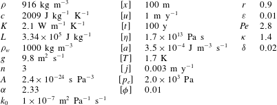
Typical values of parameters and scales for the variables.
 $[{\it\phi}]={\it\varepsilon}$
is a ‘scale’ for the porosities, which are by definition dimensionless. There is considerable uncertainty over the permeability constants
 $k_{0}$
and
 ${\it\alpha}$
, and consequently
 ${\it\kappa}$
.

As an example, we estimate values for these scalings in table 1, using a typical driving stress of approximately
 $10^{5}~\text{Pa}$
and strain rate
 $[D]\approx 0.1~\text{m}~\text{y}^{-1}$
to infer order-of-magnitude estimates of the dissipation rate
 $[a]$
and viscosity
 $[{\it\eta}]=(1/2)A^{-1/n}[D]^{1/n-1}$
. A vertical length scale of
 $100~\text{m}$
and velocity scale of
 $1~\text{m}~\text{y}^{-1}$
are used in anticipation of our one-dimensional test cases in § 4.
The resulting dimensionless parameters are
 $$\begin{eqnarray}\displaystyle r=\frac{{\it\rho}}{{\it\rho}_{w}},\quad {\it\varepsilon}=\frac{{\it\rho}c[T]}{{\it\rho}_{w}L},\quad \mathit{Pe}\,=\frac{{\it\rho}c[u][x]}{K},\quad {\it\kappa}=\frac{k_{0}{\it\varepsilon}^{{\it\alpha}}({\it\rho}_{w}-{\it\rho})g}{[j]},\quad {\it\delta}=\frac{[p_{e}]}{({\it\rho}_{w}-{\it\rho})g[x]}, & & \displaystyle \nonumber\\ \displaystyle & & \displaystyle\end{eqnarray}$$
which represent the density ratio, the porosity scale (also in this case an inverse Stefan number), the Péclet number (the ratio of advection to conduction), a permeability parameter
 ${\it\kappa}$
(a dimensionless measure of both permeability and gravity) and a compaction parameter
 ${\it\delta}$
, which measures how much compaction pressure gradients contribute to relative moisture flux.
We drop the asterisk decorations immediately with the understanding that all variables are dimensionless. The scaled versions of force balance (2.18) and constitutive law (2.19) (recall that we can reduce these to (2.2)–(2.3) in the cold domain by setting
 ${\it\phi}=D_{kk}=0$
) are
 $$\begin{eqnarray}\displaystyle & \displaystyle \frac{\partial }{\partial x_{j}}[(1-{\it\varepsilon}{\it\phi}){\it\tau}_{ij}]+\frac{{\it\varepsilon}}{\mathit{Pe}\,}\frac{\partial }{\partial x_{i}}({\it\phi}p_{e})-\frac{\partial p_{r}}{\partial x_{i}}=\frac{{\it\varepsilon}}{\mathit{Pe}\,{\it\delta}}{\it\phi}g_{i}, & \displaystyle\end{eqnarray}$$
 $$\begin{eqnarray}\displaystyle & \displaystyle {\it\tau}_{ij}=A(T,{\it\phi})D^{1/n-1}\left(\unicode[STIX]{x1D60B}_{ij}-{\textstyle \frac{1}{3}}D_{kk}{\it\delta}_{ij}\right), & \displaystyle\end{eqnarray}$$
where
 $A$
is now dimensionless.
In the cold ice domain, mass balance and conservation of energy are
 $$\begin{eqnarray}\displaystyle & \displaystyle \boldsymbol{{\rm\nabla}}\boldsymbol{\cdot }\boldsymbol{u}=0, & \displaystyle\end{eqnarray}$$
 $$\begin{eqnarray}\displaystyle & \displaystyle \mathit{Pe}\,\left(\frac{\partial T}{\partial t}+\boldsymbol{u}\boldsymbol{\cdot }\boldsymbol{{\rm\nabla}}T\right)-{\rm\nabla}^{2}T=a. & \displaystyle\end{eqnarray}$$
In the temperate domain,
 $$\begin{eqnarray}\displaystyle & \displaystyle \boldsymbol{{\rm\nabla}}\boldsymbol{\cdot }\boldsymbol{u}=-\frac{{\it\varepsilon}}{\mathit{Pe}\,}\boldsymbol{{\rm\nabla}}\boldsymbol{\cdot }\boldsymbol{j}-\frac{{\it\varepsilon}(1-r)}{r\mathit{Pe}\,}a, & \displaystyle\end{eqnarray}$$
 $$\begin{eqnarray}\displaystyle & \displaystyle \mathit{Pe}\,\left(\frac{\partial {\it\phi}}{\partial t}+\boldsymbol{u}\boldsymbol{\cdot }\boldsymbol{{\rm\nabla}}{\it\phi}+{\it\phi}\boldsymbol{{\rm\nabla}}\boldsymbol{\cdot }\boldsymbol{u}\right)+\boldsymbol{{\rm\nabla}}\boldsymbol{\cdot }\boldsymbol{j}=a, & \displaystyle\end{eqnarray}$$
 $$\begin{eqnarray}\displaystyle & \displaystyle \boldsymbol{{\rm\nabla}}\boldsymbol{\cdot }\boldsymbol{j}=\frac{{\it\phi}p_{e}}{{\it\eta}}-\frac{1-r}{r\mathit{Pe}\,}a, & \displaystyle\end{eqnarray}$$
 $$\begin{eqnarray}\displaystyle & \displaystyle \boldsymbol{j}={\it\kappa}{\it\phi}^{{\it\alpha}}\left(\boldsymbol{g}+{\it\delta}\boldsymbol{{\rm\nabla}}p_{e}+\mathit{Pe}\,{\it\delta}\boldsymbol{{\rm\nabla}}p_{r}\right), & \displaystyle\end{eqnarray}$$
 ${\it\eta}=(1/2)AD^{1/n-1}$
being a dimensionless viscosity. These represent respectively, overall mass conservation, moisture conservation, the compaction relation and Darcy’s law. The non-dimensional gravity is
 $\boldsymbol{g}=(0,0,-1)$
, assuming the axes are oriented with the
 $z$
-direction pointing vertically upwards. The jump conditions at the boundaries between cold (
 $^{-}$
) and temperate (
 $^{+}$
) domains become
 $$\begin{eqnarray}\displaystyle & \displaystyle \boldsymbol{j}^{+}\boldsymbol{\cdot }\boldsymbol{n}=-(1-r)\mathit{Pe}\,[{\it\phi}(\boldsymbol{u}-\boldsymbol{v})]^{+}\boldsymbol{\cdot }\boldsymbol{n}, & \displaystyle\end{eqnarray}$$
 $$\begin{eqnarray}\displaystyle & \displaystyle \left[(1-{\it\varepsilon}{\it\phi}){\it\tau}_{ij}+\frac{{\it\varepsilon}}{\mathit{Pe}\,}{\it\phi}p_{e}{\it\delta}_{ij}-p_{r}{\it\delta}_{ij}\right]^{+}n_{j}=({\it\tau}_{ij}-p{\it\delta}_{ij})^{-}n_{j}, & \displaystyle\end{eqnarray}$$
 $$\begin{eqnarray}\displaystyle & \displaystyle r\mathit{Pe}\,[{\it\phi}(\boldsymbol{u}-\boldsymbol{v})]^{+}\boldsymbol{\cdot }\boldsymbol{n}=-\boldsymbol{{\rm\nabla}}T^{-}\boldsymbol{\cdot }\boldsymbol{n}, & \displaystyle\end{eqnarray}$$
with
 $\boldsymbol{u}$
and
 $T$
still continuous, so
 $T=T_{m}$
. The first of these jump conditions indicates that if a finite quantity of water is carried into the boundary (and therefore freezes there and expands), mass conservation requires that there must be a compensating moisture flux away from the boundary. The second is a statement of force balance while the third is the Stefan condition, which relates freezing at the boundary to the rate of heat transfer away from it.
To complete our approximation, we now take the limits
 ${\it\varepsilon}\rightarrow 0$
, and
 $r\rightarrow 1$
.
 ${\it\varepsilon}\ll 1$
corresponds to the assumption of a low moisture content, which ensures that the flow of the ice matrix remains divergence free. This follows from (2.32), assuming
 $\mathit{Pe}\,$
does not simultaneously go to zero; so treating the ice as incompressible in this way makes sense provided the ice moves predominantly due to background flow of the ice sheet, rather than through compaction alone (the latter would be an unusual circumstance). Setting
 $r\ll 1$
implies that the effects of contraction and expansion upon melting and freezing are ignored in so far as they induce moisture movement. The effect of the density difference causing pore water to drain under gravity is still included in (2.35); this is the Boussinesq approximation.
The limit of small
 ${\it\delta}$
is also appropriate, as table 1 indicates that
 ${\it\varepsilon}$
and
 ${\it\delta}$
are typically of similar size. We choose to retain the term
 ${\it\delta}\boldsymbol{{\rm\nabla}}p_{e}$
in the definition of
 $\boldsymbol{j}$
for now, as it leads to the formation of boundary layers, as discussed in § 4 and appendix D. These boundary layers involve large gradients in
 $p_{e}$
, but not gradients in
 $p_{r}$
, as the latter is prescribed from the ice flow solution. We can therefore legitimately omit the term
 $\mathit{Pe}\,{\it\delta}\boldsymbol{{\rm\nabla}}p_{r}$
in (2.35), provided the Péclet number is not too large. Specifically, we shall assume that
 $1\gg \mathit{Pe}\,{\it\delta}\gg {\it\epsilon}$
, which allows us also to omit the right-hand side of (2.28).
2.5 Summary
Here we summarize the reduced model. At leading order the equations for ice flow, to be solved in both cold and temperate domains, are
 $$\begin{eqnarray}\displaystyle & \displaystyle \boldsymbol{{\rm\nabla}}\boldsymbol{\cdot }\boldsymbol{u}=0, & \displaystyle\end{eqnarray}$$
 $$\begin{eqnarray}\displaystyle & \displaystyle \frac{\partial {\it\tau}_{ij}}{\partial x_{j}}-\frac{\partial p_{r}}{\partial x_{i}}=0, & \displaystyle\end{eqnarray}$$
 $$\begin{eqnarray}\displaystyle {\it\tau}_{ij}=2{\it\eta}\unicode[STIX]{x1D60B}_{ij},\quad {\it\eta}=\frac{1}{2}A(T,{\it\phi})^{-1/n}D^{1/n-1},\quad \unicode[STIX]{x1D60B}_{ij}=\frac{1}{2}\left(\frac{\partial u_{i}}{\partial u_{j}}+\frac{\partial u_{j}}{\partial x_{i}}\right),\quad D=\sqrt{\unicode[STIX]{x1D60B}_{ij}\unicode[STIX]{x1D60B}_{ij}/2}. & & \displaystyle \nonumber\\ \displaystyle & & \displaystyle\end{eqnarray}$$
The energy equation for cold ice is
 $$\begin{eqnarray}\displaystyle \mathit{Pe}\,\left(\frac{\partial T}{\partial t}+\boldsymbol{u}\boldsymbol{\cdot }\boldsymbol{{\rm\nabla}}T\right)-{\rm\nabla}^{2}T=a,\quad {\it\phi}=0,\quad T\leqslant T_{m}, & & \displaystyle\end{eqnarray}$$
where
 $a={\it\tau}_{ij}\unicode[STIX]{x1D60B}_{ij}$
and the equivalent equations for temperate ice are
 $$\begin{eqnarray}\displaystyle \mathit{Pe}\,\left(\frac{\partial {\it\phi}}{\partial t}+\boldsymbol{u}\boldsymbol{\cdot }\boldsymbol{{\rm\nabla}}{\it\phi}\right)+\boldsymbol{{\rm\nabla}}\boldsymbol{\cdot }\boldsymbol{j}=a,\quad T=T_{m},\quad {\it\phi}>0, & & \displaystyle\end{eqnarray}$$
 $$\begin{eqnarray}\displaystyle \boldsymbol{{\rm\nabla}}\boldsymbol{\cdot }\boldsymbol{j}=\frac{{\it\phi}p_{e}}{{\it\eta}}, & & \displaystyle\end{eqnarray}$$
 $$\begin{eqnarray}\displaystyle \boldsymbol{j}={\it\kappa}{\it\phi}^{{\it\alpha}}\left(\boldsymbol{g}+{\it\delta}\boldsymbol{{\rm\nabla}}p_{e}\right). & & \displaystyle\end{eqnarray}$$
The conditions to apply at the cold–temperate boundaries are
 $$\begin{eqnarray}\displaystyle & \displaystyle \boldsymbol{j}^{+}\boldsymbol{\cdot }\boldsymbol{n}=0, & \displaystyle\end{eqnarray}$$
 $$\begin{eqnarray}\displaystyle & \displaystyle \mathit{Pe}\,[{\it\phi}(\boldsymbol{u}-\boldsymbol{v})]^{+}\boldsymbol{\cdot }\boldsymbol{n}=-\boldsymbol{{\rm\nabla}}T^{-}\boldsymbol{\cdot }\boldsymbol{n}, & \displaystyle\end{eqnarray}$$
 $$\begin{eqnarray}\displaystyle & \displaystyle T^{-}=T_{m}. & \displaystyle\end{eqnarray}$$
Note that the temperature and porosity equations in the cold and temperate regions can be combined as an enthalpy equation in the usual way. The dimensionless enthalpy is defined as
 $h=T+{\it\phi}$
, and conversely temperature and porosity are derived from this as
 $$\begin{eqnarray}\displaystyle \left.\begin{array}{@{}ll@{}}T=h,{\it\phi}=0, & \text{if}~h<T_{m},\\ T=T_{m},{\it\phi}=h-T_{m}, & \text{if}~h\geqslant T_{m}.\end{array}\right\} & & \displaystyle\end{eqnarray}$$
Then (2.42) and (2.43) are equivalent to
 $$\begin{eqnarray}\displaystyle \mathit{Pe}\,\left(\frac{\partial h}{\partial t}+\boldsymbol{u}\boldsymbol{\cdot }\boldsymbol{{\rm\nabla}}h\right)+\boldsymbol{{\rm\nabla}}\boldsymbol{\cdot }\boldsymbol{Q}=a,\quad \boldsymbol{Q}=\left\{\begin{array}{@{}ll@{}}-\boldsymbol{{\rm\nabla}}T,\quad & h<T_{m},\\ \boldsymbol{j},\quad & h\geqslant T_{m}.\end{array}\right. & & \displaystyle\end{eqnarray}$$
Enthalpy is transported by advection and conduction in the cold ice and by advection and moisture transport in the temperate ice. The Stefan condition (2.47) is the natural jump condition that arises from treating this equation in weak form (e.g. Ockendon et al. Reference Ockendon, Howison, Lacey and Movchan2003, § 2.5).
3 Boundary and jump conditions
Boundary conditions at the exterior boundaries and the interior cold–temperate transitions require careful consideration, and they have understandably attracted much attention and debate in the literature (Fowler & Larson Reference Fowler and Larson1978; Hutter Reference Hutter1982; Fowler Reference Fowler1984; Aschwanden et al. Reference Aschwanden, Bueler, Khroulev and Blatter2012).
Under the approximation
 ${\it\varepsilon}\rightarrow 0$
, we have retained incompressibility throughout the domain, so that the ice flow problem (2.39)–(2.41) is solved everywhere. Any coupling of the ice velocity
 $\boldsymbol{u}$
to the thermal problem occurs through the flow-law parameter
 $A$
, or through the boundary conditions (for instance, if the basal friction law depends on temperature). This ice flow problem requires boundary conditions on the stress or velocity components at all exterior boundaries, but since these are quite standard we do not discuss them further. Instead, we concentrate on the conditions to be applied to the temperature and moisture problems.
3.1 Interior boundaries
The interior boundaries between cold and temperate regions are free boundaries, whose position must be determined as part of the problem. Their location is determined from the condition
 $T=T_{m}$
, along with the jump condition (2.47). The manner in which these conditions operate depends upon the direction of ice flow relative to the boundary.
In particular, since
 $T\leqslant T_{m}$
in the cold region and
 $\boldsymbol{n}$
is defined to point into the temperate region, we always have
 $\boldsymbol{{\rm\nabla}}T^{-}\boldsymbol{\cdot }\boldsymbol{n}\geqslant 0$
, and (2.47) therefore implies that
 ${\it\phi}(\boldsymbol{u}-\boldsymbol{v})^{+}\boldsymbol{\cdot }\boldsymbol{n}\leqslant 0$
. If ice flows from a cold to a temperate region, so
 $(\boldsymbol{u}-\boldsymbol{v})\boldsymbol{\cdot }\boldsymbol{n}>0$
(we refer to this an ‘inflow’ boundary), then this is only possible if
 ${\it\phi}^{+}=0$
. Consequently (2.47) implies that in fact
 $\boldsymbol{{\rm\nabla}}T^{-}\boldsymbol{\cdot }\boldsymbol{n}=0$
. Thus, at any inflow boundary, (2.47) actually requires
 ${\it\phi}=\boldsymbol{{\rm\nabla}}T\boldsymbol{\cdot }\boldsymbol{n}=0$
. The condition
 ${\it\phi}=0$
seems intuitive, meaning that ice entering the temperate region starts with no water content. From the perspective of the heat transport problem on the cold side, the boundary is both at the melting temperature
 $T=T_{m}$
and has zero diffusive heat flux
 $-\boldsymbol{{\rm\nabla}}T\boldsymbol{\cdot }\boldsymbol{n}$
across it.
These two conditions are equivalent to the conditions applied for a parabolic obstacle problem, with
 $T\leqslant T_{m}$
defining the obstacle; this is the approach to defining the cold–temperate boundary implicit in the models of Zwinger et al. (Reference Zwinger, Greve, Gagliardini, Shiraiwa and Lyly2007) and Suckale et al. (Reference Suckale, Platt, Perol and Rice2014). With these boundary conditions, the temperature problem decouples from the physics of the temperate region
 ${\it\Omega}^{+}$
.
However, at an outflow boundary (where
 $(\boldsymbol{u}-\boldsymbol{v})\boldsymbol{\cdot }\boldsymbol{n}\leqslant 0$
), unlike an inflow boundary, the boundary conditions on temperature do not decouple from those on the temperate ice side. There can be a discontinuity in
 ${\it\phi}$
, and the jump condition (2.47) relates this discontinuity to the jump in temperature gradient, in the usual manner of a Stefan condition. This reflects the fact that freezing can occur at an outflow boundary. From the point of view of determining the location of the boundary, the porosity in the temperate region needs to be solved for primarily because it features in this condition. The obstacle problem formulation mentioned above is only appropriate when there are no outflow boundaries.
The jump condition for mass conservation (2.46) provides the necessary boundary condition for the moisture transport problem (2.44)–(2.45) which, for a given instantaneous porosity field
 ${\it\phi}$
, constitutes an elliptic (Helmholtz-like) problem for
 $p_{e}$
, explicitly
 $$\begin{eqnarray}\displaystyle \boldsymbol{{\rm\nabla}}\boldsymbol{\cdot }\left[{\it\kappa}{\it\phi}^{{\it\alpha}}\left(g+{\it\delta}\boldsymbol{{\rm\nabla}}p_{e}\right)\right]-\frac{{\it\phi}p_{e}}{{\it\eta}}=0. & & \displaystyle\end{eqnarray}$$
The equivalent conditions for this problem when the temperate domain extends to the exterior boundary will be discussed below. However, it is worth pointing out that the elliptic nature of this problem means that the divergence term
 $\boldsymbol{{\rm\nabla}}\boldsymbol{\cdot }\boldsymbol{j}$
in (2.43) acts as a non-local function of the porosity field. The remaining hyperbolic part of that equation suggests that a boundary condition is only required for
 ${\it\phi}$
on the ‘inflow’ parts of the boundary, which is precisely where the above discussion around (2.47) revealed that
 ${\it\phi}=0$
.
3.2 Exterior boundaries
The conditions to apply at external boundaries of the domain depend on whether the ice adjacent to the boundary is temperate or cold. In some cases, this distinction may be prescribed as part of the boundary condition (e.g. if the temperature is prescribed to be below the melting point), whilst in others (e.g. if a given heat flux is supplied) it needs to be determined as part of the problem through the imposition of the constraint
 $T\leqslant T_{m}$
at the boundary, and may change in time.
At cold exterior boundaries, a condition on temperature or temperature gradient (or a relation between them) must be prescribed, in the usual way. Naturally, no conditions are required for the moisture transport problem there.
At temperate exterior boundaries, the appropriate conditions again depend on whether they are ‘inflow’ or ‘outflow’ boundaries, with
 $(\boldsymbol{u}-\boldsymbol{v})\boldsymbol{\cdot }\boldsymbol{n}$
being positive or negative respectively. Here the normal
 $\boldsymbol{n}$
points into the temperate region, and
 $\boldsymbol{v}$
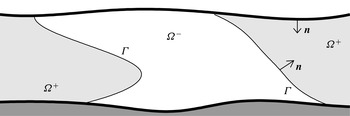
is the velocity of the boundary itself (see figure 1). In the case of an inflow boundary, the porosity
 ${\it\phi}$
must be prescribed, as well as a condition on either the moisture flux
 $\boldsymbol{j}\boldsymbol{\cdot }\boldsymbol{n}$
or the compaction pressure
 $p_{e}$
for the moisture transport problem (2.34)–(2.35). In the case of an outflow boundary, only a condition on
 $\boldsymbol{j}\boldsymbol{\cdot }\boldsymbol{n}$
or
 $p_{e}$
is required.
Temperate and cold domains,
 ${\it\Omega}^{+}$
and
 ${\it\Omega}^{-}$
, respectively, separated by interior boundaries
 ${\it\Gamma}$
with normal
 $\boldsymbol{n}$
. Thick lines correspond to exterior boundaries.

For example, at the surface of a temperate glacier, the accumulation region corresponds to an inflow boundary, and we may expect to prescribe the porosity and the moisture flux
 $\boldsymbol{j}\boldsymbol{\cdot }\boldsymbol{n}$
, possibly as the output of a model for the compacting firn layer above. In the ablation region, where the surface corresponds to an outflow boundary, the compaction pressure
 $p_{e}$
is likely to be zero, with both the pore pressure and ice pressure being atmospheric. (There is in fact a possible complication that arises here: the pore pressure
 $p_{w}$
cannot drop below atmospheric pressure or, in isolation from the atmosphere, below the triple point pressure of water. This bound may be attained near the glacier surface and lead to a region of partially saturated temperate ice overlying saturated temperate ice, and hence the introduction of another free boundary. The appropriate extension of our model to this case is likely to be similar to an analogous situation in subglacial drainage (Schoof, Hewitt & Werder Reference Schoof, Hewitt and Werder2012), but we do not pursue this further here.)
At the base of a temperate glacier, where basal melting occurs, we have an outflow boundary. A single boundary condition is required. The obvious choice is to equate the englacial water pressure
 $p_{w}$
with subglacial water pressure. If we define effective pressure at the bed
 $N$
as normal stress minus subglacial water pressure, then in dimensionless terms
 $$\begin{eqnarray}\displaystyle p_{e}=N+\mathit{Pe}\,{\it\tau}_{nn}, & & \displaystyle\end{eqnarray}$$
where
 ${\it\tau}_{nn}$
is the dimensionless deviatoric normal stress at the bed (the difference between
 $p_{e}$
and
 $N$
arises because the definition of compaction pressure does not take account of deviatoric stresses or the normal direction to the bed).
If basal freeze-on occurs (for example due to decompression and supercooling of subglacial water), the boundary would be of inflow type, and we additionally expect to apply a condition on the porosity of the frozen-on ice. The porosity condition would presumably depend on precisely how the frozen-on ice is formed; if frazil ice is formed in the subglacial water and accumulates mechanically at the underside of the glacier, a non-zero porosity may result, while direct freeze-on to the base of the glacier may result in a zero porosity boundary condition. Again, we do not investigate the physics involved further here.
4 Steady-state test cases
Next, we consider the solution of our polythermal ice model in a simple, one-dimensional setting in steady state. Most of the examples we use should be thought of as the modelling equivalent of a controlled experiment rather than an attempt to reproduce realistic ice sheet conditions; one of the scenarios we consider is the polythermal equivalent of the highly idealized temperature solution for an ice divide due to Robin (Reference Robin1955). As explained in the introduction, we wish to illustrate the generic behaviour of solutions to our model, and to test different solution methods against each other.
We consider a parallel-sided slab of ice, with the
 $z$
-axis oriented perpendicular to the slab, and assume that temperature, porosity and compaction pressure are functions of
 $z$
only. The divergence-free velocity field
 $\boldsymbol{u}$
and dissipation rate
 $a$
are assumed to be prescribed. For most of the solutions below, we simply take
 $\boldsymbol{u}$
to be constant and let
 $u$
denote the
 $z$
-component of
 $\boldsymbol{u}$
.
The dissipation rate
 $a$
will generally be treated as constant, even though this is not consistent with a constant velocity field. (A shearing term parallel to the sides of the slab can always be added to generate a constant
 $a$
while keeping the
 $z$
-component
 $u$
unchanged, or other sources of heating could be appealed to.) The case of a position-dependent dissipation rate
 $a=a(z)\geqslant 0$
could be handled just as easily by our solution methods, but adds no significant insight. For simplicity, we also set
 $T_{m}=0$
and assume the case of a constant dimensionless viscosity
 ${\it\eta}=1$
.
In steady state, all time derivatives as well as the migration velocity
 $\boldsymbol{v}$
of the cold–temperate boundary vanish. The steady-state version of the polythermal ice problem in § 2.5 can be written in one-dimensional form as
 $$\begin{eqnarray}\displaystyle \mathit{Pe}\,u\frac{\text{d}T}{\text{d}z}-\frac{\text{d}^{2}T}{\text{d}z^{2}}=a & & \displaystyle\end{eqnarray}$$
subject to
 $T\leqslant 0$
for the cold subdomain
 ${\it\Omega}^{-}$
, and
 $$\begin{eqnarray}\displaystyle & \displaystyle \mathit{Pe}\,u\frac{\text{d}{\it\phi}}{\text{d}z}+{\it\phi}p_{e}=a, & \displaystyle\end{eqnarray}$$
 $$\begin{eqnarray}\displaystyle & \displaystyle \mathit{Pe}\,u\frac{\text{d}{\it\phi}}{\text{d}z}+\frac{\text{d}}{\text{d}z}\left[{\it\kappa}{\it\phi}^{{\it\alpha}}\left(g+{\it\delta}\frac{\text{d}p_{e}}{\text{d}z}\right)\right]=a, & \displaystyle\end{eqnarray}$$
 ${\it\phi}>0$
in the temperate subdomain
 ${\it\Omega}^{+}$
, where
 $g$
is the
 $z$
-component of gravity. In our solutions, we take
 $z$
to be oriented upward, so
 $g=-1$
.
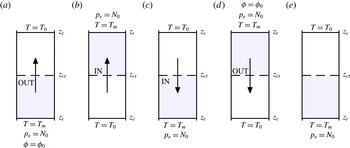
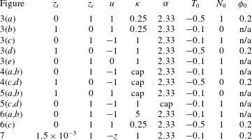
Steady-state test problems considered, labelled with the exterior boundary conditions, corresponding to the solutions shown in figure 3. Shading corresponds to the temperate ice region, and the arrow indicates the direction of constant ice motion. Gravity acts downwards.

We impose that the slab has one cold boundary and one temperate boundary, at
 $z=z_{c}$
and
 $z=z_{t}$
, respectively, with a single temperate region
 ${\it\Omega}^{+}$
adjacent to
 $z_{t}$
, and a single cold region
 ${\it\Omega}^{-}$
adjacent to
 $z_{c}$
, separated by a cold–temperate boundary point
 $z=z_{ct}$
(see figure 2). We must distinguish between cases in which
 $z=z_{ct}$
is an inflow or an outflow boundary (see § 3). For an inflow boundary at
 $z=z_{ct}$
(where
 $\text{sgn}(u)=\text{sgn}(z_{t}-z_{ct})$
at
 $z=z_{ct}$
), the cold–temperate boundary conditions now state that temperature is at the melting point, while conductive heat transport, moisture transport and porosity vanish at the boundary:
 $$\begin{eqnarray}\displaystyle T=-\frac{\text{d}T}{\text{d}z}=q={\it\phi}=0\quad \text{at }z=z_{ct}, & & \displaystyle\end{eqnarray}$$
where we define
 $q$
to be the
 $z$
-component of total moisture (or enthalpy) flux,
 $$\begin{eqnarray}\displaystyle q=\mathit{Pe}\,u{\it\phi}+{\it\kappa}{\it\phi}^{{\it\alpha}}\left(g+{\it\delta}\frac{\text{d}p_{e}}{\text{d}z}\right). & & \displaystyle\end{eqnarray}$$
Conversely, for an outflow boundary (
 $\text{sgn}(u)=\text{sgn}(z_{ct}-z_{t})$
), we have one fewer boundary condition than for the inflow case,
 $$\begin{eqnarray}\displaystyle T=0,\quad -\frac{\text{d}T}{\text{d}z}=q=\mathit{Pe}\,u{\it\phi}\quad \text{at }z=z_{ct}, & & \displaystyle\end{eqnarray}$$
again stating that temperature is at the melting point, while conductive heat flux equals the moisture-based enthalpy flux, and, in the form of the last equality, that the relative moisture (or Darcy) flux vanishes: note from (4.3b
) that
 $q-\mathit{Pe}\,u{\it\phi}$
is simply the
 $z$
-component of relative moisture flux
 $\boldsymbol{j}$
.
At the cold exterior boundary
 $z=z_{c}$
, we prescribe a temperature
 $$\begin{eqnarray}\displaystyle T=T_{0}, & & \displaystyle\end{eqnarray}$$
where naturally
 $T_{0}<0$
. The necessary boundary conditions at the temperate exterior boundary
 $z=z_{t}$
depend on whether this is an inflow or an outflow boundary. The nature of the boundary at
 $z_{t}$
is simply the reverse of that at
 $z_{ct}$
(we assume that
 $u$
does not change sign). Thus, an inflow boundary at
 $z=z_{ct}$
corresponds to an outflow boundary at
 $z=z_{t}$
, and we simply prescribe an effective pressure
 $$\begin{eqnarray}\displaystyle p_{e}=N_{0}. & & \displaystyle\end{eqnarray}$$
Conversely, an outflow boundary at
 $z=z_{ct}$
corresponds to an inflow boundary at
 $z=z_{t}$
, which also requires a condition on porosity at
 $z_{t}$
; in that case, we impose
 $$\begin{eqnarray}\displaystyle {\it\phi}={\it\phi}_{0} & & \displaystyle\end{eqnarray}$$
in addition to (4.4b
). Having an additional boundary condition at
 $z=z_{t}$
accounts for having one fewer at
 $z_{ct}$
, as pointed out above.
The six boundary conditions specified (one at
 $z_{c}$
and either three or four at
 $z_{ct}$
, corresponding to one or two at
 $z_{t}$
, respectively) allow us to solve the second-order problem (4.1) along with the coupled first/second-order system (4.2), while also determining the free boundary position
 $z_{ct}$
. As we show in the supplementary material, there appears to be no problem in applying this counting argument despite the fact that
 ${\it\phi}=0$
at the cold–temperate boundary for the inflow case, which makes (4.2b
) singular.
We solve the steady-state problem in three ways: first, we use a finite volume solver for the time-dependent temperate ice problem (appendix A), running the solution to a steady state where the latter exists. Secondly, we use a multiple shooting method to solve the steady-state boundary value problem (appendix B). In addition to direct numerical solution techniques, we also compute an asymptotic approximation to the solution valid for a small compaction parameter
 ${\it\delta}$
. Omitting the pressure-gradient term
 ${\it\delta}\text{d}/\text{d}z({\it\kappa}{\it\phi}^{{\it\alpha}}\text{d}p_{e}/\text{d}z)$
from (4.2b
) leads to a simple first-order problem for
 ${\it\phi}$
,
 $$\begin{eqnarray}\displaystyle \left(\mathit{Pe}\,u+{\it\alpha}{\it\kappa}{\it\phi}^{{\it\alpha}-1}g\right)\frac{\text{d}{\it\phi}}{\text{d}z}=a, & & \displaystyle\end{eqnarray}$$
which can be integrated from the relevant inflow boundary (either
 $z_{t}$
or
 $z_{ct}$
) at which
 ${\it\phi}$
is prescribed. The compaction pressure can then be computed a posteriori from (4.2a
) as
 $$\begin{eqnarray}\displaystyle p_{e}=\frac{{\it\alpha}{\it\kappa}{\it\phi}^{{\it\alpha}-2}ga}{\mathit{Pe}\,u+{\it\alpha}{\it\kappa}{\it\phi}^{{\it\alpha}-1}g}. & & \displaystyle\end{eqnarray}$$
Note that this is actually a special case of a more general hyperbolic problem we can motivate by omitting the
 $O({\it\delta})$
pressure-gradient term from the definition of moisture flux. From (2.43) and (2.45), this leads to
 $$\begin{eqnarray}\mathit{Pe}\,\frac{\partial {\it\phi}}{\partial t}+\boldsymbol{{\rm\nabla}}\boldsymbol{\cdot }\left(\mathit{Pe}\,\boldsymbol{u}{\it\phi}+{\it\kappa}{\it\phi}^{{\it\alpha}}\boldsymbol{g}\right)=a.\end{eqnarray}$$
In reducing the problem from (4.2b
) to (4.5), we have however omitted higher-order derivatives in
 $p_{e}$
, which leads to difficulties in satisfying all the boundary conditions. For instance, if we have a cold–temperate outflow boundary, we can legitimately use (4.5) to find a leading-order solution for the boundary location
 $z_{ct}$
though the first equality in (4.3c
)
 $_{2}$
, at leading order
 $$\begin{eqnarray}\displaystyle \left.-\frac{\text{d}T}{\text{d}z}\right|_{z=z_{ct}}=q(z_{ct})=\mathit{Pe}\,u(z_{ct}){\it\phi}(z_{ct})+{\it\kappa}{\it\phi}(z_{ct})^{{\it\alpha}}g. & & \displaystyle\end{eqnarray}$$
However, we will not generally be able to satisfy the last equality in (4.3c
)
 $_{2}$
, stating that the relative moisture flux
 $q-\mathit{Pe}\,u{\it\phi}$
should simultaneously vanish. To ensure the latter, a boundary layer becomes necessary in which gradients in compaction pressure cannot be neglected. There are different types of boundary layers at different types of boundaries (depending on whether they are cold–temperate or exterior boundaries, and whether they are of inflow or outflow type). We describe them in brief in appendix D and in greater detail in the supplementary material.
Unless explicitly stated otherwise, the asymptotic solutions we present below are composite solutions of (4.5) and (4.6) combined with the relevant boundary layer solutions (Holmes Reference Holmes1995). When comparing asymptotic solutions with numerical solutions of the ‘full’ model, the latter were generally computed from the multiple shooting method.
5 Results
5.1 Cold–temperate inflow and outflow boundaries
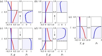
Generically, there are four different cases to consider: ice can flow up or down, and at the same time it can flow from cold to temperate or temperate to cold. Some of these combinations may not be widespread in ice sheets: for instance, cold ice moving upward into a temperate region is likely to be an exotic situation. An example of each of these four cases is illustrated in figure 3, where we plot the solution obtained from the finite volume solver using dots, the shooting method solution as a solid line and the asymptotic solution as a dashed line. Note that all three solution methods agree well. The finite volume and shooting solutions are essentially identical, indicating that the numerical methods work well in computing steady-state solutions. Despite a finite value of
 ${\it\delta}=1.25\times 10^{-2}$
in each case, the asymptotic solution differs perceptibly only for the case shown in panel (a). We show in § 5.5 that the difference between the numerical and asymptotic solutions shrinks as
 ${\it\delta}$
is made smaller.
Generic steady-state solutions. Each subplot labelled (a)–(e) shows
 ${\it\phi}$
(red) and
 $T$
(blue) on the left,
 $p_{e}$
(blue) on the right.
 $z$
is plotted along the vertical. A solid line is the shooting method solution, dots indicate the steady-state finite volume solution (not all cell centre values are shown), a dashed line the asymptotic solution; these are mostly indistinguishable. The arrow between the panels in each case indicates the ice flow direction; no arrow in subplot (e) indicates that there is no advection across the slab.
 $\boldsymbol{g}$
points down. Shading indicates the temperate subdomain. In each case
 ${\it\delta}=1.25\times 10^{-2}$
. The remaining parameter values for each plot are given in table 2.

Ice flowing from the cold into the temperate region corresponds to an inflow boundary, at which porosity
 ${\it\phi}$
and temperature gradient
 $\text{d}T/\text{d}z$
both vanish, so that the enthalpy content and flux are continuous (in figure 3
b,c). This is the case captured by the obstacle problem formulation of Zwinger et al. (Reference Zwinger, Greve, Gagliardini, Shiraiwa and Lyly2007). Conversely, ice flowing from the temperate into the cold subdomain creates an outflow boundary (figure 3
a,d), at which a Stefan condition ensures continuity of a non-zero enthalpy flux, while the enthalpy content is discontinuous:
 ${\it\phi}$
does not go to zero at the cold–temperate boundary in that case. This case cannot be described by an obstacle problem formulation, as the temperature gradient
 $\text{d}T/\text{d}z$
also no longer vanishes at the cold–temperate boundary. Other than the discontinuity in porosity at the cold–temperate boundary for outflow cases, the other main difference between cold–temperate inflow and outflow boundaries is the spike in effective pressure near the cold–temperate boundary visible in the outflow cases in figure 3(a,d). The need to satisfy a zero Darcy flux boundary condition, combined with a non-vanishing porosity at the boundary, result in large compaction pressure gradients in outflow cases, which can be explained through the boundary layer structure summarized in appendix D. In order to show all solutions at the same scale, we have cut off part of the compaction pressure plots in figure 3(a,d); note that
 $p_{e}$
remains finite in both cases.
Parameter values used in the figures. In all cases,
 $\mathit{Pe}\,=a=1$
,
 $g=-1$
.
 ${\it\delta}$
is indicated in the figure captions. ‘cap’ also indicates that the relevant value is indicated in the figure caption (typically because more than one value is used in the figure), n/a indicates a value is not needed.

The main difference we see at this point between upward- and downward-moving ice is in the porosity gradients in the ice and in the sign of the compaction pressure. For downward-moving ice, advective and gravity-driven moisture transport reinforce each other, and the same amount of moisture flux requires a smaller porosity than when gravity opposes advection. This results in porosity growing more slowly away from the cold–temperate inflow boundary when ice flow is down rather than up (compare in figure 3 b,c). The different rates of growth in porosity away from these boundaries also require different compaction pressures. When gravity opposes upward advection, compaction pressures are typically negative to ensure that porosities can grow fast enough, while in cases where advection is in the downward direction, positive compaction pressures ensure that porosity remains sufficiently small.
In addition to inflow and outflow cases, we have also plotted a solution for the marginal case of no advection in the vertical (
 $u=0$
) in figure 3(e). This case, which also shares many of the characteristics of the temperate ice behaviour for large permeabilities
 ${\it\kappa}$
(see § 5.2), is appropriate for a parallel-sided slab of ice flowing in simple shear (the introductory text book example of the flow of an infinitely long glacier). The mathematical details of this case are given in appendix C. At the cold–temperate boundary, we have the same ‘obstacle problem’ boundary conditions of zero conductive flux and temperature at the melting point as are appropriate to the inflow case; in other words, the temperature problem and the determination of the boundary location
 $z_{ct}$
once more decouple from the problem of finding porosity and compaction pressure. By contrast with the inflow case, however, porosity at the cold–temperate boundary does not vanish, attaining a small but finite value (for small
 ${\it\delta}$
), while compaction pressure is largest at the top of the temperate subdomain (while still remaining finite) and decreases towards the bottom.
5.2 The role of relative moisture flux
Here we consider the effects of increasing the permeability parameter
 ${\it\kappa}$
. We focus on the case where velocity
 $u$
and gravity
 $g$
have the same orientation, so advective and gravity-driven moisture flux combine to increase total transport.
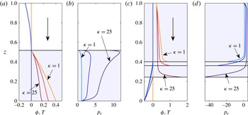
Figure 4(a,b) shows steady-state solutions computed for downward ice flow from the cold subdomain into the temperate subdomain for different values of
 ${\it\kappa}$
. The cold–temperate boundary is then an inflow boundary at which temperature
 $T$
as well as the advective heat flux
 $-T_{z}$
both vanish. As a result, the location of the cold–temperate boundary is unaffected by changing permeability: the temperature problem decouples from the porosity and compaction pressure problem.
The effect of increasing
 ${\it\kappa}$
. Same basic plotting scheme as in figure 3(c,d), here showing only the shooting method solution. Asymptotic solutions are omitted to make the plot less crowded. The large vertical arrow indicates ice flow direction. (a,b) Cold ice overlying temperate ice. Solution for
 ${\it\kappa}=1$
shown in orange/turquoise,
 ${\it\kappa}=5$
in red/blue and
 ${\it\kappa}=25$
in maroon/dark blue. Here
 ${\it\delta}=1.25\times 10^{-2}$
. Other parameter values are given in table 2. Panels (c,d) show analogous solutions (same colour scheme) for cold ice underlying warm ice. The horizontal black lines show
 $z=z_{ct}$
for different
 ${\it\kappa}$
, the shading is for
 ${\it\kappa}=25$
.

In the temperate subdomain, however, changing the permeability
 ${\it\kappa}$
does have a substantial effect on porosity and compaction pressure. As the cold–temperate boundary location does not depend on
 ${\it\kappa}$
, the same amount of melt is produced in each case, but increased permeability leads to lower porosities. The increased ability of water to drain through the matrix, in addition to downward transport along with the moving ice, allows the same amount of water to be transported at lower porosities. Gravity-driven moisture flux through the ice matrix is the main way in which our model departs from more widely used enthalpy-gradient methods, and this clearly has the ability to reduce the amounts of moisture stored in temperate ice. Lower porosities can only be maintained by faster compaction in the temperate ice matrix, which explains why the compaction pressure increases with
 ${\it\kappa}$
.
If we turn to the case of temperate ice being advected downwards into a cold region (see figure 4
c,d), similar observations apply: except in a boundary layer near the cold–temperate boundary, porosity decreases and compaction pressure increases as we increase
 ${\it\kappa}$
. The boundary layer (see appendix D.2) behaves differently because this is where moisture draining downwards becomes backed up due to the fact that the relative moisture flux must vanish at the cold–temperate boundary. The notable difference from the previous case is that the temperature and location of the cold–temperate boundary are no longer decoupled in this situation. The total moisture flux
 $q$
differs between the cases computed with different values of
 ${\it\kappa}$
, and as a result, the cold–temperate boundary location also differs: larger permeability
 ${\it\kappa}$
leads to more moisture draining down from the upper boundary, which reduces the size of the cold subdomain and increases the temperature gradients there.
5.3 Upwards advection and the breakdown of steady-state solutions
A different situation altogether arises when ice moves upwards (figure 3(a,b), in which case downward gravity-driven drainage through the matrix opposes upward advective transport. An increase in the ice permeability coefficient
 ${\it\kappa}$
can lead to the breakdown of the steady-state solution. In the case of temperate ice lying above cold ice, the ice enters the temperate subdomain with zero porosity. Upward transport has to increase as we go up from the boundary to account for the moisture that is being produced. At small porosities, that transport has to occur predominantly through advection, leading to an increase in porosity (recall that we assume that
 ${\it\alpha}\geqslant 2$
). As porosity increases, however, the tendency for moisture to drain downward also increases, making it harder to evacuate the moisture being produced.
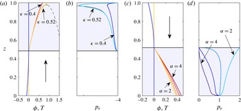
Same basic plotting scheme as in figure 3, showing: (a,b) solutions for upward ice advection with values of
 ${\it\kappa}$
close to the breakdown of steady-state solutions; and (c,d) solutions for downward ice advection showing the effect of changing
 ${\it\alpha}$
at the inflow boundary. The shooting method and composite asymptotic solutions are shown (they are essentially indistinguishable). In (a,b), solutions are for
 ${\it\kappa}=0.4$
(red/blue),
 ${\it\kappa}=0.52$
(orange/turquoise), while the black curve shows the asymptotic (‘outer’) solution that solves (4.5) with no boundary layers for
 ${\it\kappa}=0.52$
. Here
 ${\it\delta}=1.25\times 10^{-4}$
. In (c,d), solutions are for
 ${\it\alpha}=2$
(orange/turquoise), 2.33 (light red/light blue), 3 (red/blue) and 4 (maroon/dark blue) and
 ${\it\delta}=1.25\times 10^{-3}$
. See table 2 for the remaining parameters.

In fact, if we ignore the role of pressure gradients, then there is a maximum attainable upward moisture flux. A steady state cannot be reached if total moisture production in the domain exceeds this maximum flux: water starts to accumulate inside the domain instead. This is more likely to happen if
 ${\it\kappa}$
is larger, which facilitates downward drainage and reduces the maximum flux.
Figure 5(a,b) shows two examples of this situation for values of
 ${\it\kappa}$
small enough that the steady-state solution still exists. For the larger value
 ${\it\kappa}=0.52$
, the steady state is very close to breakdown, and for larger values we find there is no steady state. In fact if we were to set
 ${\it\delta}$
to zero with
 ${\it\kappa}=0.52$
there would be no steady solution in that case either; the maximum flux mentioned above is achieved just beneath the upper boundary, but the pressure gradients in a boundary layer enable moisture transport over the remaining short distance to the exterior boundary (this is only possible if the maximum flux is reached within an
 $O({\it\delta}^{2/5})$
distance from the boundary, see appendix D.1).
This phenomenon is easy to understand mathematically. Take (4.5) with
 $u$
constant. In steady state, the moisture flux must be
 $q=a(z-z_{ct})$
, related to
 ${\it\phi}$
through
 $q=\mathit{Pe}\,u{\it\phi}+{\it\kappa}g{\it\phi}^{{\it\alpha}}$
(in the limit
 ${\it\delta}\rightarrow 0$
). Equating these two expressions allows us to solve for
 ${\it\phi}$
, leading to the solid black line in figure 5(a) (the dashed black line also solves
 $\mathit{Pe}\,u{\it\phi}+{\it\kappa}{\it\phi}^{{\it\alpha}}g=a(z-z_{ct})$
, but does not satisfy
 ${\it\phi}(z_{ct})=0$
). If
 $u$
is positive and
 $g$
negative, then
 $q({\it\phi})$
has a maximum of
 $$\begin{eqnarray}\displaystyle q_{max}=\frac{({\it\alpha}-1)}{{\it\alpha}}\left[\frac{(\mathit{Pe}\,u)^{{\it\alpha}}}{-{\it\alpha}{\it\kappa}g}\right]^{1/({\it\alpha}-1)} & & \displaystyle\end{eqnarray}$$
reached at
 ${\it\phi}=[\mathit{Pe}\,u/(-{\it\alpha}{\it\kappa}g)]^{1/({\it\alpha}-1)}$
. If the maximum flux
 $a(z_{t}-z_{ct})$
demanded by mass conservation is larger than
 $q_{max}$
, then the simplified model does not permit a steady state. Clearly this happens if
 ${\it\kappa}$
is made too large since
 $q_{max}$
decreases with
 ${\it\kappa}$
. As shown in figure 5(a,b), it is possible to find steady-state solutions for values of
 ${\it\kappa}$
slightly larger than this argument would suggest, but not for substantially larger ones. For values of
 ${\it\kappa}$
larger than approximately
 $0.53$
and the remaining parameters as used in figure 5, a wave, or multiple waves, in porosity and compaction pressure form first near the top of the domain and slowly move downwards, growing as they move downwards (see Spiegelman (Reference Spiegelman1993) for a similar phenomenon in the theory of melt extraction from mantle rock). This rather complicated phenomenon will be explored in more detail in a separate paper.
We have illustrated the breakdown mechanism for cold ice moving upwards into temperate ice. In the case of ice moving upward from a temperate exterior domain
 $z_{t}$
that lies below the cold domain, a similar loss of steady state can occur, but since solutions then depend on precisely what boundary condition
 ${\it\phi}_{0}$
is specified at the lower boundary we avoid this additional complication here.
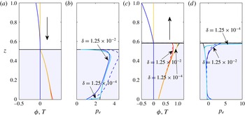
Comparison of full and asymptotic solutions. Same basic plotting scheme as in earlier figures, showing the shooting method (solid) and composite asymptotic solutions (dashed). The ‘outer’ solution to (4.5) with no boundary layers is shown in black. (a,b): solution for downward-moving ice with
 ${\it\delta}=1.25\times 10^{-2}$
(turquoise/orange) and
 ${\it\delta}=1.25\times 10^{-4}$
(blue/red). Other parameter values are given in table 2. (c,d) Show corresponding solutions for upward-moving ice, same colour scheme. Note the obvious discrepancies between asymptotic and full solutions at
 ${\it\delta}=1.25\times 10^{-2}$
, while they are practically indistinguishable for the smaller value. The discrepancies mostly manifest themselves in
 $p_{e}$
rather than
 ${\it\phi}$
.

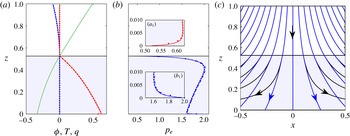
Solution with a non-constant velocity (5.2). Same basic plotting scheme as before, showing the finite volume (solid circles), shooting method (solid) and composite asymptotic solutions (dashed).
 ${\it\delta}=1.25\times 10^{-3}$
, and other parameter values are given in table 2. (a)
 $T$
in blue,
 ${\it\phi}$
in red and
 $q$
in green. (In the earlier solutions with constant velocity
 $u$
, the graph of
 $q$
is simply a straight line, and therefore omitted.) (b)
 $p_{e}$
in blue. (
 $\mathit{a}_{1}$
) and (
 $\mathit{b}_{1}$
) are enlargements of (a) and (b) near the bottom of the domain, showing the narrow boundary layers there. Panel (c) shows corresponding streamlines for ice flow (solid black) and moisture flow (dashed blue) in the two spatial dimensions.

5.4 Behaviour near cold–temperate inflow boundaries: dependence of permeability on porosity
A limitation of our model is that we do not have much information about the permeability of temperate ice. This affects not only our ability to estimate
 ${\it\kappa}$
, but also the dependence of permeability on porosity, parameterized here through a power law with exponent
 ${\it\alpha}$
. A choice of
 ${\it\alpha}=2$
arises if flow through temperate ice is limited by veins (triple grain junctions) while most of the moisture is stored at the nodes where multiple veins meet (Nye & Frank Reference Nye and Frank1973), while
 ${\it\alpha}=3$
can be seen as the natural small porosity limit of the Carman–Kozeny relationship (Bear & Bachmat Reference Bear and Bachmat1990). The choice of
 ${\it\alpha}$
can have a significant effect on our solutions, especially the compaction pressure distribution. This is particularly pronounced at inflow boundaries, where the elliptic problem (3.1) for
 $p_{e}$
becomes singular. In figure 5(c,d), we show solutions with a cold–temperate inflow boundary, keeping all parameter values but
 ${\it\alpha}$
constant (note that comparing values of
 ${\it\kappa}$
for different exponents
 ${\it\alpha}$
is however meaningless).
Qualitatively, the main difference we find is that compaction pressure near the inflow boundary increases with decreasing
 ${\it\alpha}$
. For
 ${\it\alpha}\geqslant 3$
, compaction pressures near the inflow boundary increase continuously from zero, whereas for smaller values of
 ${\it\alpha}$
, finite compaction pressures can occur at the boundary (we have limited our computations to
 ${\it\alpha}\geqslant 2$
, for which compaction pressure remains finite near the inflow boundary). A detailed analysis of the near-boundary behaviour is given in the supplementary material.
5.5 Comparison with asymptotic solutions
Figures 3 and 5 display the asymptotic solution along with the direct numerical solutions for relatively small values of the compaction parameter
 ${\it\delta}$
. Here we investigate more systematically how well the asymptotic solution agrees with the direct numerical solution as we alter
 ${\it\delta}$
, and describe the effect this has on the boundary layers that form in the temperate region. We focus on two cases, both with cold ice overlying temperate ice (as is most realistic for glaciers and ice sheets).
Figure 6 shows a solution for downward-moving ice in (a,b) and for the upward-moving case in (c,d). In each, solutions are plotted for
 ${\it\delta}=1.25\times 10^{-2}$
and
 ${\it\delta}=1.25\times 10^{-4}$
. Dashed coloured lines show the composite asymptotic solutions (computed from (4.5) and the appropriate boundary layer models describing the behaviour near
 $z_{t}$
and
 $z_{ct}$
), and solid lines show steady states calculated from the shooting method. The black line (mostly obscured behind the full
 ${\it\delta}=1.25\times 10^{-4}$
solution) is the asymptotic solution without any boundary layers (that is, the ‘outer’ solution that was also plotted in figure 5).
In both cases, the asymptotic solution is indistinguishable from the shooting method solution at
 ${\it\delta}=1.25\times 10^{-4}$
, but distinct at
 ${\it\delta}=1.25\times 10^{-2}$
, showing the expected convergence in the limit of small
 ${\it\delta}$
. The error is generally smaller for
 ${\it\phi}$
than for
 $p_{e}$
. For
 ${\it\delta}=1.25\times 10^{-2}$
, the latter error is considerably larger for the case of downward-flowing ice in figure 3(b) than for upward-flowing ice in figure 3(d). This is partially the result of the calculation for downward-flowing ice having been done with a larger value of
 ${\it\kappa}$
which in general leads to worse agreement between the asymptotic solution and the full solution for fixed
 ${\it\delta}$
. This would have been quite apparent in figure 4 had we included the asymptotic solutions there.
One a technical note, it appears that for
 ${\it\delta}=1.25\times 10^{-2}$
, the outer solution (black) actually agrees better with the full solution (blue) than the dashed composite solution in figure 3(b). This results from the boundary layer solution near
 $z_{ct}$
(appendix D.3), which gives more accurate results very close to the boundary but decays too slowly to give good composite solutions for moderate
 ${\it\delta}$
; omitting this boundary layer generally gives closer agreement except near
 $z_{ct}$
, where the fractional error becomes large if the boundary layer is omitted. Note that the boundary layer is only relevant when
 $2<{\it\alpha}<3$
, which applies for the solution shown in figure 6.
Quite generally, the composite solution also becomes more similar to the outer solution in the limit of small
 ${\it\delta}$
. This happens because the boundary layers shrink in extent: most of the boundary layers are of thickness
 $O({\it\delta}^{1/2})$
, the main exception being the case of a cold–temperate inflow boundary as described in appendix D. The boundary layers do, however have quite a distinct character, most notably in how compaction pressure behaves near the boundaries. Near the exterior boundary
 $z=z_{t}=0$
, there is a boundary layer in which
 $p_{e}$
departs by an
 $O(1)$
fraction from the outer solution in order to match the prescribed boundary condition (appendix D.1), while the boundary layer near the cold–temperate boundary has much larger
 $O({\it\delta}^{-1/2})$
excursions in compaction pressure if the boundary is an outflow boundary (to ensure the zero Darcy flux condition is met, see appendix D.2), and a much smaller correction if it is an inflow boundary (see appendix D.3), which in any case is required only when
 $2<{\it\alpha}<3$
(where the correction in
 $p_{e}$
is of
 $O({\it\delta}^{({\it\alpha}-2)/(3-{\it\alpha})})$
, while
 $p_{e}$
in the outer solution goes to zero near the boundary). We remind the reader that the boundary layer structure is also discussed in much greater detail in the supplementary material.
5.6 An ice divide solution
Here we present an extension of the temperature solution for an idealized ice divide (the central ridge that separates flow towards different parts of the ice sheet margin) due to Robin (Reference Robin1955) to the polythermal case. Instead of using a constant velocity
 $\boldsymbol{u}$
, we assume the velocity field
 $\boldsymbol{u}$
to be of the form
 $$\begin{eqnarray}\displaystyle \boldsymbol{u}=(x,0,-z), & & \displaystyle\end{eqnarray}$$
giving a linear change in velocity across the slab with depth while ensuring that
 $\boldsymbol{{\rm\nabla}}\boldsymbol{\cdot }\boldsymbol{u}=0$
. With the domain lying above
 $z>0$
, (5.2) replicates the idealized ice divide velocity field in Robin (Reference Robin1955).
We still use
 $u=-z$
to denote
 $z$
-component of the velocity field in this case. As before, it is perfectly consistent to assume that
 ${\it\phi}$
,
 $p_{e}$
and
 $q$
depend only on
 $z$
. Because we never previously assumed that
 $u$
was a constant (the only constraints actually being that
 $u$
depends on
 $z$
only, and does not change sign in the domain), the entire steady-state model of § 4, including the simplified hyperbolic model (4.5), applies without change to the new velocity field (5.2). This is true so long as we do not allow the point
 $z=0$
to lie inside the temperate subdomain
 ${\it\Omega}^{+}$
, so that
 $u$
cannot change sign and inflow boundaries at
 $z_{ct}$
still correspond to outflow boundaries at
 $z_{t}$
, and vice versa. (In fact, when solving for the steady states using the shooting method of appendix B, we do not allow
 $z=0$
to lie on the boundary of the domain either, to prevent the advection problem (4.2a
) becoming singular with
 $u=0$
, and use a small but finite
 $z_{t}$
.)
Figure 7 shows an example of a solution. One crucial difference from the previous examples is that the underlying velocity field is now intrinsically two-dimensional, allowing moisture transport in the transverse direction. Unlike the examples above, this also implies that the
 $z$
-component of total moisture flux
 $q$
need not depend linearly on
 $z$
, as part of the moisture produced can be evacuated through sideways advection rather than through vertical moisture transport. Figure 7 therefore shows the now non-trivial solution for
 $q$
(taken to be the total vertical enthalpy transport in both subdomains, i.e.
 $q=\mathit{Pe}\,uT-\text{d}T/\text{d}z$
in the cold domain) plotted along with
 ${\it\phi}$
and
 $p_{e}$
.
Near the base of the ice, vertical advection becomes very small, and lateral advection reduces the (negative) size of the flux
 $q$
: sideways transport starts to play a more significant role as the vertical velocity field
 $u$
becomes small. The other main qualitative difference with previous solutions lies in the boundary layer near the temperate exterior boundary
 $z_{t}$
: these turn out to be much narrower, occupying only a small region (of thickness
 $O({\it\delta})$
) near the base of the ice, in which effective pressure and porosity change rapidly (see the insets in figure 7
b).
6 Discussion and conclusions
We have developed a model for polythermal ice incorporating gravity- and pressure-gradient-driven moisture transport through a viscously compacting ice matrix. Our model is essentially a stripped-back form of the theory suggested by Fowler (Reference Fowler1984), although his boundary conditions are subtly different from ours. The main advantage of our formulation is that it is directly applicable to most ice flow models, in that it retains the incompressibility of ice and allows a standard Stokes flow solver (or its equivalent for ice flow models using a reduced version of the Stokes equations) to be used to find ice velocity, while still using Darcy’s law to account for the transport of moisture relative to the ice matrix. This stands in contrast with other approaches that use a diffusive constitutive relation for relative moisture flux, or allow no such flux at all. In particular, the fact that our model allows gravity to remove moisture from the temperate subdomain may prevent the excessive build-up of porosity.
We have used a finite volume discretization to solve the model, using an enthalpy method to capture the free boundary between cold and temperate ice (appendix A) without having to resort to the diffusive flux of an enthalpy gradient method. We have tested this solution method against a multiple shooting method that allows direct numerical solution of the steady-state equations as a one-dimensional free-boundary problem. The results obtained from the two methods are virtually indistinguishable, giving us confidence in the performance of both.
The numerical solutions have allowed us to explore the relatively diverse phenomenology of solutions. The most relevant difference between the solutions we have shown is intrinsic to the basic model, namely the difference between boundaries where cold ice flows through the cold–temperate boundary into the temperate domain (‘inflow’ problems) or vice versa (‘outflow’ problems). The effective boundary conditions at the cold–temperate boundary change depending on whether we have inflow or outflow at the cold–temperate boundary: at an inflow boundary, conductive heat flux and porosity vanish (so the enthalpy is continuous), while at an outflow boundary, porosity can instead be finite and a Stefan condition determines the non-zero conductive heat flux in terms of porosity and advection velocity.
To be more precise, both boundary conditions ultimately derive from the same Stefan condition, but the need to satisfy inequality constraints on
 $T$
and
 ${\it\phi}$
near an inflow boundary leads to the conclusion that conductive heat flux and porosity both vanish at inflow boundaries, while the same Stefan condition permits discontinuities in porosity at outflow boundaries. The ‘obstacle problem’ formulation implicit in Zwinger et al. (Reference Zwinger, Greve, Gagliardini, Shiraiwa and Lyly2007) and Suckale et al. (Reference Suckale, Platt, Perol and Rice2014), which requires zero conductive heat flux at the cold–temperate boundary, is therefore appropriate if there are only inflow boundaries, or (in an approximate way) if porosities are minimized at outflow boundaries, for instance by gravity-driven drainage, but not otherwise.
The other main difference between our sample solutions, apart from that between inflow and outflow solutions, lies in the direction of ice flow relative to gravity, which determines whether ice advection reinforces or opposes gravity-driven drainage. In the case of upward advection, larger permeabilities can lead to the breakdown of steady states as water becomes trapped in the domain through gravity-driven drainage, while larger permeabilities in the case of downward advection simply lead to smaller porosities and higher compaction pressures.
Different choices of power-law exponent
 ${\it\alpha}$
in the definition of permeability lead to different distributions of compaction pressure, especially near cold–temperate inflow boundaries. There is at present little experimental data on the permeability of temperate ice and its dependence on porosity, which is an obvious target for future research.
One of the practically useful results of this paper has also been that we have generally found good agreement between the full model and an asymptotic solution based on the limit of
 ${\it\delta}\ll 1$
, which leads to the simpler hyperbolic model (4.7). This allows us potentially to reconcile our model with the established enthalpy gradient models that are already in use in ice sheet simulations.
The standard enthalpy-gradient method (Aschwanden et al.
Reference Aschwanden, Bueler, Khroulev and Blatter2012) is most applicable to near-impermeable temperate ice, in which case it provides a diffusive regularization of the purely advective transport of moisture that would result in our model from setting
 ${\it\kappa}=0$
. The introduction of the diffusive term
 $\boldsymbol{j}=-{\it\nu}\boldsymbol{{\rm\nabla}}{\it\phi}$
with small but positive
 ${\it\nu}$
leads to porosity (and therefore enthalpy) going to zero at the cold–temperate boundary even where this is an outflow boundary in our parlance, while there is a discontinuity at such a boundary for purely advective transport. However, the discrepancy between the two models is then limited to a diffusive boundary layer near outflow boundaries of thickness
 $O({\it\nu})$
, and using the diffusive regularization introduces a comparable
 $O({\it\nu})$
error into the location of the free boundary and the computation of moisture content.
The standard enthalpy-gradient method however does not account for physically realistic drainage of moisture through the matrix with a non-zero permeability
 ${\it\kappa}>0$
, which may be key to preventing undue build-up of moisture content. Our asymptotic model, (4.7), suggests a plausible extension of the enthalpy-gradient method that incorporates at least gravity-driven drainage. In particular, we can define enthalpy as in (2.49) through
 $h=T$
for
 $T<T_{m}$
and
 $h=T_{m}+{\it\phi}$
for
 $T=T_{m}$
, and formulate the following enthalpy-gradient model,
 $$\begin{eqnarray}\displaystyle \mathit{Pe}\,\left(\frac{\partial h}{\partial t}+\boldsymbol{u}\boldsymbol{\cdot }\boldsymbol{{\rm\nabla}}h\right)+\boldsymbol{{\rm\nabla}}\boldsymbol{\cdot }\boldsymbol{Q}=a,\quad \boldsymbol{Q}=\left\{\begin{array}{@{}ll@{}}-\boldsymbol{{\rm\nabla}}h\quad & \text{for }h\leqslant T_{m}\\ {\it\kappa}\boldsymbol{g}(h-T_{m})^{{\it\alpha}}-{\it\nu}\boldsymbol{{\rm\nabla}}h\quad & \text{for}\,h>T_{m},\end{array}\right. & & \displaystyle\end{eqnarray}$$
which should be understood in its ‘weak’ form (given its diffusive nature, meaning that both
 $h$
and the normal component of
 $\boldsymbol{Q}$
will be continuous across the cold–temperate boundary). The model (6.1) is a diffusively regularized version of the asymptotic model for enthalpy transport (4.7).
The difference between this version and our full polythermal ice model, as described in § 2, lies in replacing the pressure-gradient-driven flux term
 ${\it\delta}{\it\kappa}{\it\phi}^{{\it\alpha}}\boldsymbol{{\rm\nabla}}p_{e}$
by
 $-{\it\nu}\boldsymbol{{\rm\nabla}}h$
in the temperate subdomain, which inevitably will lead to discrepancies near the cold–temperate boundary. The relevant boundary layers will differ from each other, but the hyperbolic ‘outer’ problems away from such boundary layers in general have the same solution. The resulting errors will generally be localized near the boundaries of the temperate subdomain, and both models should in general predict the location of the cold–temperate boundary to within a small (
 $O({\it\nu},{\it\delta})$
) error of each other. The applicability of (6.1) is therefore limited to cases where such small errors in locating the cold–temperate boundary are acceptable.
A diffusive model such as (6.1) may in fact be appropriate in a different physical limit to the one considered so far. Recall that we excluded surface energy effects from consideration in (2.15), and outlined a generalization in (2.16), which we did not however pursue further. It is conceivable that, rather than having a balance between advection, melting and closure of void space as in (2.15), there could be a leading-order balance between compaction pressure
 $p_{e}$
and the surface energy term
 $p_{s}({\it\phi})$
in (2.16), so
 $p_{e}=p_{s}({\it\phi})$
and the relative moisture flux becomes
 $\boldsymbol{Q}={\it\kappa}{\it\phi}^{{\it\alpha}}(\boldsymbol{g}+{\it\delta}\boldsymbol{{\rm\nabla}}p_{s}({\it\phi}))$
, which is of the same form as (6.1) if we put
 ${\it\nu}=-{\it\delta}{\it\kappa}{\it\phi}^{{\it\alpha}}\text{d}p_{s}/\text{d}{\it\phi}>0$
.
There are some further subtleties that may need careful handling: for instance, the diffusive model (6.1) is not able to handle the breakdown of solutions described in § 5.3 or, more generally, problems in which (4.7) predicts the formation of shocks: it can be shown that the diffusively smoothed version of (4.7) that arises from (6.1) behaves very differently in that case from our full model in § 2. These situations, which we will study in more detail elsewhere, are however unlikely to be widespread in ice sheets. Where they are absent, (6.1) provides a straightforward mechanism for adapting existing enthalpy-gradient models to incorporate some of the physics studied in this paper.
In closing, we emphasize the need for further experimental work to complement model development. For instance, our work has assumed a permeability of the form
 $k_{0}{\it\phi}^{{\it\alpha}}$
, where neither
 $k_{0}$
nor
 ${\it\alpha}$
are particularly well constrained by measurements (although
 ${\it\alpha}=2$
is a widely used limit for the case where moisture is mostly stored at the nodes of a network of veins, with the veins themselves controlling permeability). The need for experimental data is likely to become more acute if we include the effect of surface energy on compaction as described in equation (2.16): we would need a constitutive relation for the surface energy term
 $p_{s}({\it\phi})$
. These are clearly important questions for future research.
Acknowledgements
C.G.S. acknowledges the support of NSERC grants 357193-13 and 446042-13 and a Killam Faculty Research Fellowship at UBC. I.J.H. is supported by a Marie Curie FP7 Career Integration Grant within the 7th European Union Framework Programme. We thank the three anonymous referees and the editor, G. Worster, for their thorough scrutiny, and one referee in particular for drawing our attention to surface energy effects in limiting compaction.
Supplementary material
Supplementary material is available at http://dx.doi.org/10.1017/jfm.2016.251.
Appendix A. Finite volume method
The thermal and moisture equations can be written succinctly as
 $$\begin{eqnarray}\displaystyle & \displaystyle \mathit{Pe}\,\left(\frac{\partial h}{\partial t}+\boldsymbol{u}\boldsymbol{\cdot }\boldsymbol{{\rm\nabla}}h\right)={\rm\nabla}^{2}T+a-\frac{{\it\phi}p_{e}}{{\it\eta}},\quad \text{on}~{\it\Omega}, & \displaystyle\end{eqnarray}$$
 $$\begin{eqnarray}\displaystyle & \displaystyle \boldsymbol{{\rm\nabla}}\boldsymbol{\cdot }\boldsymbol{j}\equiv \boldsymbol{{\rm\nabla}}\boldsymbol{\cdot }\left[{\it\kappa}{\it\phi}^{{\it\alpha}}\left(\boldsymbol{g}+{\it\delta}\boldsymbol{{\rm\nabla}}p_{e}\right)\right]=\frac{{\it\phi}p_{e}}{{\it\eta}},\quad \text{on}~{\it\Omega}^{+}, & \displaystyle\end{eqnarray}$$
where the enthalpy is related to temperature and porosity by
 $$\begin{eqnarray}\displaystyle h=T+{\it\phi}\quad \text{and}\quad \left\{\begin{array}{@{}ll@{}}T=h,{\it\phi}=0,\quad & \text{on}~{\it\Omega}^{-},\\ T=T_{m},{\it\phi}=h-T_{m},\quad & \text{on}~{\it\Omega}^{+},\end{array}\right. & & \displaystyle\end{eqnarray}$$
and where
 ${\it\Omega}^{+}$
is defined by where
 $h>T_{m}$
, and
 ${\it\Omega}^{-}$
where
 $h\leqslant T_{m}$
.
The first equation (A 1) applies throughout the entire domain, provided we formally extend the definition of
 $p_{e}$
to be finite in the cold domain (the final term corresponding to the moisture divergence
 $\boldsymbol{{\rm\nabla}}\boldsymbol{\cdot }\boldsymbol{j}$
is only effective when
 ${\it\phi}>0$
). Provided this equation is solved with a conservative numerical scheme, the Stefan condition
 $\mathit{Pe}\,{\it\phi}^{+}(\boldsymbol{v}-\boldsymbol{u})\boldsymbol{\cdot }\boldsymbol{n}=-\boldsymbol{{\rm\nabla}}T^{-}\boldsymbol{\cdot }\boldsymbol{n}$
is automatically satisfied at the free boundaries. Boundary conditions are applied for
 $T$
on the cold exterior boundaries
 $\partial {\it\Omega}^{-}$
, and for
 ${\it\phi}$
on the inflow portions of the temperate boundaries
 $\partial {\it\Omega}^{+}$
. Equation (A 2) applies only in the temperate ice, with condition
 $\boldsymbol{j}\boldsymbol{\cdot }\boldsymbol{n}=0$
on
 ${\it\Gamma}$
and with a condition for
 $\boldsymbol{j}={\it\kappa}{\it\phi}^{{\it\alpha}}\left(\boldsymbol{g}+{\it\delta}\boldsymbol{{\rm\nabla}}p_{e}\right)$
or
 $p_{e}$
on
 $\partial {\it\Omega}^{+}$
.
Our procedure to solve these equations uses a finite volume discretization and a simple operator splitting method. Temperature, porosity and pressure are discretized on a regular grid, while ice velocity and moisture flux
 $\boldsymbol{j}$
are defined on a staggered grid. Using a harmonic average to define the permeability on the staggered grid means that the condition
 $\boldsymbol{j}\boldsymbol{\cdot }\boldsymbol{n}=0$
is naturally applied at any cold–temperate boundary. The discretized domain is partitioned into
 ${\it\Omega}^{+}$
and
 ${\it\Omega}^{-}$
explicitly at each time step according to the current value of
 $h$
. The elliptic equation (A 2) is solved on
 ${\it\Omega}^{+}$
to determine
 $p_{e}$
given the current
 ${\it\phi}$
, and the energy equation (A 1) is then advanced for
 $h$
with a combination of implicit and explicit discretization. Specifically, the left-hand side is treated with an upwind discretization, the temperature on the right-hand side is set equal to
 $h$
and discretized implicitly on the current
 ${\it\Omega}^{-}$
, but set equal to
 $T_{m}$
on
 ${\it\Omega}^{+}$
, and the final compaction term is discretized explicitly. The new value of
 $h$
then defines the new
 $T$
and
 ${\it\phi}$
as well as the new domain partition.
Appendix B. The shooting method for the temperate ice problem
The steady-state heat equation (4.1) is straightforward to solve through the use of integrating factors. For constant
 $u$
, we have
 $$\begin{eqnarray}\displaystyle T(z)=\frac{az}{\mathit{Pe}\,u}+A\exp (\mathit{Pe}\,uz)+B, & & \displaystyle\end{eqnarray}$$
while for the linear velocity profile (5.2), we obtain a more complicated formula in terms of Dawson’s integrals (see supplementary material). In both cases,
 $T(z)$
can be stated in closed form, with two constants of integration
 $A$
and
 $B$
. One constraint on
 $A$
and
 $B$
arises from the Dirichlet condition (4.4a
), while further constraints arise from the coupling between the temperate ice problem with the solution of the heat equation at
 $z=z_{ct}$
.
A closed form solution of the temperate ice problem (4.2) is not possible, but we can render it in a form suitable for a shooting method approach. Straightforward manipulations allow the one-dimensional problem (4.2) for temperate ice to be reformulated as a first-order system
 $$\begin{eqnarray}\displaystyle & \displaystyle \frac{\text{d}{\it\phi}}{\text{d}z}=\frac{a-{\it\phi}p_{e}}{\mathit{Pe}\,u}, & \displaystyle\end{eqnarray}$$
 $$\begin{eqnarray}\displaystyle & \displaystyle \frac{\text{d}p_{e}}{\text{d}z}={\it\delta}^{-1}\left(\frac{q}{{\it\kappa}{\it\phi}^{{\it\alpha}}}-\frac{\mathit{Pe}\,u}{{\it\kappa}{\it\phi}^{{\it\alpha}-1}}-g\right), & \displaystyle\end{eqnarray}$$
 $$\begin{eqnarray}\displaystyle & \displaystyle \frac{\text{d}q}{\text{d}z}=a+\mathit{Pe}\,{\it\phi}\frac{\text{d}u}{\text{d}z}. & \displaystyle\end{eqnarray}$$
 $N$
partitions of the temperate domain. This turns the solution into a root-finding problem, as we need to determine the correct ‘initial’ conditions at the starting point of each partition, such that the solution is continuous at each partition endpoint that is interior to the temperate domain and such that the boundary conditions at
 $z_{t}$
and
 $z_{ct}$
are satisfied. The root-finding problem, which we solve using Newton’s method, involves not only finding the ‘initial’ conditions for the system (B 2), but also the constants of integration
 $A$
and
 $B$
and the cold–temperate boundary location
 $z_{ct}$
.
A difficulty arises in solving the system (B 2) near a cold–temperate inflow boundary at
 $z=z_{ct}$
. In that case
 ${\it\phi}$
vanishes at the boundary and (B 2b
) becomes singular. We amend the shooting method above by solving a transformed system of equations in the partition of the domain closest to
 $z_{ct}$
in that case, using the transformed variables
 $$\begin{eqnarray}\displaystyle z-z_{ct}={\it\phi}^{{\it\nu}}{\it\chi},\quad {\it\Psi}={\it\phi}^{{\it\beta}}N,\quad {\it\omega}=[q-a(z-z_{ct})]/{\it\phi},\quad \frac{\text{d}{\it\zeta}}{\text{d}z}={\it\phi}^{-{\it\gamma}}, & & \displaystyle\end{eqnarray}$$
with for
 $2\leqslant {\it\alpha}\leqslant 3$
, we use
 ${\it\nu}={\it\gamma}=1$
,
 ${\it\beta}={\it\alpha}-2$
and
 ${\it\nu}=1$
,
 ${\it\beta}={\it\gamma}=({\it\alpha}-1)/2$
for
 ${\it\alpha}>3$
. This transforms the problem of integrating up to the boundary at
 $z=z_{ct}$
into the problem of finding an orbit into a fixed point of a dynamical system as
 $\text{sgn}(u(z_{ct}))\times {\it\zeta}\rightarrow -\infty$
. For details on the transformation, and the shooting method in general, see the supplementary material.
Appendix C. Temperate ice without advection
With no advection in the
 $z$
-direction, (4.2a
) degenerates into the algebraic relation
 ${\it\phi}=a/p_{e}$
and (4.2b
) becomes
 $$\begin{eqnarray}\frac{\text{d}q}{\text{d}z}=a,\quad q={\it\kappa}\left(\frac{a}{p_{e}}\right)^{{\it\alpha}}\left(g+{\it\delta}\frac{\text{d}p_{e}}{\text{d}z}\right).\end{eqnarray}$$
At the cold–temperate boundary, we now have neither an inflow nor an outflow boundary, but the combination of a vanishing Darcy flux and the Stefan condition in steady state require inflow-type boundary conditions on flux and temperature (but not porosity):
 $$\begin{eqnarray}T=-\frac{\text{d}T}{\text{d}z}=q=0.\end{eqnarray}$$
The boundary conditions on
 $T$
once again take the form appropriate for an obstacle problem, and finding the free boundary
 $z_{ct}$
decouples from the problem of determining porosity and compaction pressure.
The zero Darcy flux condition allows us to integrate (C 1) to find
 $q=a(z-z_{ct})$
, and a first-order problem for
 $p_{e}$
 $$\begin{eqnarray}{\it\delta}\frac{\text{d}p_{e}}{\text{d}z}=\frac{(z-z_{ct})p_{e}^{{\it\alpha}}}{{\it\kappa}a^{{\it\alpha}-1}}-g,\end{eqnarray}$$
which must be integrated from the exterior boundary, at which
 $p_{e}=N_{0}$
. An asymptotic outer solution for small
 ${\it\delta}$
can again be found, this time in closed form, by setting the left-hand side to zero:
 $$\begin{eqnarray}p_{e}=\left(\frac{g{\it\kappa}a^{{\it\alpha}-1}}{z-z_{ct}}\right)^{1/{\it\alpha}}.\end{eqnarray}$$
With
 $g<0$
, this only has a real solution if the temperate domain lies below
 $z_{ct}$
: in the absence of advection, a steady state requires water to be able to drain downwards under gravity out of the domain. This is an extreme example of the solution breakdown discussed in § 5.3: with no advection,
 $q_{max}$
is zero and for small
 ${\it\delta}$
, there can be no steady-state solutions in which temperate ice overlies cold ice.
We elaborate on the relevant boundary layers in the asymptotic solution near
 $z_{t}$
and
 $z_{ct}$
in appendix D.
Appendix D. Asymptotic solutions
The ‘outer’ part of the asymptotic solution can be found by integrating (4.5) from whichever end of the temperate subdomain has a porosity condition imposed. This is
 $z_{ct}$
for an inflow problem, and
 $z_{t}$
otherwise. Where
 $z_{ct}$
is an outflow boundary, its location is determined by finding
 $q$
from the outer solution and equating it to
 $-\text{d}T/\text{d}z$
at
 $z_{ct}$
. A range of different boundary layers is necessary to satisfy the remaining boundary conditions. We simply state the relevant boundary layers below, and give a more expansive derivation in the supplementary material.
D.1 Exterior boundary
Near
 $z_{t}$
, let
 $\hat{n}=(z-z_{t})/{\it\delta}^{1/2}$
,
 $\hat{p}_{e}(\hat{n})=p_{e}(z)$
,
 $\hat{{\it\phi}}(\hat{n})={\it\phi}(z)$
. Then
 $\hat{{\it\phi}}\sim {\it\phi}(z_{t})$
, and
 $$\begin{eqnarray}\displaystyle \hat{p}_{e}=p_{e}(z_{t})+(N_{0}-p_{e}(z_{t}))\exp \left(-{\it\lambda}|\hat{n}|\right),\quad \text{where}~{\it\lambda}=\sqrt{\frac{\mathit{Pe }\,u(z_{t})+{\it\alpha}{\it\kappa}{\it\phi}(z_{t})^{{\it\alpha}-1}g}{\mathit{Pe}\,u(z_{t}){\it\kappa}{\it\phi}(z_{t})^{{\it\alpha}}}}, & & \displaystyle \nonumber\\ \displaystyle & & \displaystyle\end{eqnarray}$$
where
 $p_{e}(z_{t})$
and
 ${\it\phi}(z_{t})$
are the outer solutions that satisfy (4.5) and (4.6) This works well (
 ${\it\lambda}$
must be real, which requires
 $\text{sgn}[u(z_{t})]=\text{sgn}[\mathit{Pe}\,u(z_{t})+{\it\alpha}{\it\kappa}g{\it\phi}(z_{t})^{{\it\alpha}-1}]$
) unless
 $u(z_{ct})$
or
 $\mathit{Pe}\,u(z_{t})+{\it\alpha}{\it\kappa}{\it\phi}(z_{t})^{{\it\alpha}-1}g$
are small in the outer solution.
For
 $u(z_{t})\sim O({\it\delta})$
, we need to define instead
 $\acute{n} =(z-z_{t})/{\it\delta}$
,
 $\acute{{\it\phi}}(\acute{n} )={\it\phi}(z)$
,
 $\acute{p}_{e}(\acute{n} )=p_{e}(z)$
. Putting
 $\acute{u} =u(z_{t})/{\it\delta}$
,
 $\acute{u} _{z}=\text{d}u/\text{d}z$
, with
 $\acute{u}$
and
 $\acute{u} _{z}$
both of
 $O(1)$
. Then
 $$\begin{eqnarray}\displaystyle \frac{\text{d}\acute{{\it\phi}}}{\text{d}\acute{n} }=\frac{a-\acute{{\it\phi}}\acute{p}_{e}}{\mathit{Pe}\,(\acute{u} +\acute{u} _{z}\acute{n} )},\quad \frac{\text{d}\acute{p}_{e}}{\text{d}\acute{n} }=\frac{\acute{q}}{{\it\kappa}\acute{{\it\phi}}^{{\it\alpha}}}-g, & & \displaystyle\end{eqnarray}$$
where
 $\acute{q}={\it\kappa}{\it\phi}(z_{t})^{{\it\alpha}}g$
is the moisture flux at the boundary in the outer solution, and, assuming an outflow boundary at
 $z_{t}$
,
 $\acute{p}_{e}=N_{0}$
at
 $\acute{n} =0$
and
 $\acute{{\it\phi}}\rightarrow {\it\phi}(z_{t})$
as
 $\acute{n} \rightarrow \infty$
. This alternative boundary layer is needed to deal with the Robin (Reference Robin1955)-type velocity field (5.2).
Conversely, if
 $\mathit{Pe}\,u+{\it\alpha}{\it\kappa}{\it\phi}^{{\it\alpha}-1}g=O({\it\delta}^{1/5})$
near the boundary or the outer solution breaks down (
 $\mathit{Pe}\,u+{\it\alpha}{\it\kappa}{\it\phi}^{{\it\alpha}-1}g=0$
inside the domain, with
 ${\it\phi}$
computed from (4.5)) within a distance
 $O({\it\delta}^{2/5})$
of the boundary, the following alternative boundary layer model is needed: identify a point
 $z_{f}$
such that
 $\mathit{Pe}\,u(z_{f})+{\it\alpha}{\it\kappa}{\it\phi}(z_{f})^{{\it\alpha}-1}g=0$
, extending
 $u$
and therefore (4.5) smoothly past the domain boundary if needed. Put
 $\grave{u} =u(z_{f})$
,
 ${\it\phi}_{c}={\it\phi}(z_{f})$
, and define
 $\grave{n}=(z-z_{t})/{\it\delta}^{2/5}$
,
 $\grave{{\it\phi}}(\grave{n})={\it\phi}(z)$
,
 $\grave{p}_{e}(\grave{n})={\it\delta}^{1/5}p_{e}(z)$
. Then
 $\grave{{\it\phi}}={\it\phi}_{c}+{\it\delta}^{1/5}{\it\phi}^{(1)}$
, and
 $$\begin{eqnarray}\displaystyle & \displaystyle \frac{1}{2}{\it\kappa}g{\it\alpha}({\it\alpha}-1){\it\phi}_{c}^{{\it\alpha}-2}\left.\grave{{\it\phi}}^{(1)}\right.^{2}+{\it\kappa}{\it\phi}_{c}^{{\it\alpha}}\frac{\text{d}\grave{p}_{e}}{\text{d}\grave{n}}=a(\grave{n}-\grave{n}_{0}), & \displaystyle\end{eqnarray}$$
 $$\begin{eqnarray}\displaystyle & \displaystyle \mathit{Pe}\,\grave{u} \frac{\text{d}\grave{{\it\phi}}^{(1)}}{\text{d}\grave{n}}+{\it\phi}_{c}\grave{p}_{e}=0, & \displaystyle\end{eqnarray}$$
where
 $\grave{n}_{0}=(z_{f}-z_{t})/{\it\delta}^{2/5}$
is
 $O(1)$
.
 $\grave{p}_{e}\rightarrow 0$
as
 $\text{sgn}(z_{t}-z_{ct})\times \grave{n}\rightarrow \infty$
and
 $\grave{p}_{e}=0$
at
 $\grave{n}=0$
(though in practice we apply
 $\grave{p}_{e}={\it\delta}^{1/5}N_{0}$
to get a more accurate solution). This boundary layer model applies only if
 $z_{t}$
is an outflow boundary. It corresponds to the near breakdown solution in figure 5(a,b).
For the case of no advection in (C 3) with outer solution (C 4), the boundary layer at the exterior boundary is obtained by defining
 ${\check{n}}=(z-z_{t})/{\it\delta}$
,
 $\check{p}_{e}({\check{n}})=p_{e}(z)$
, so that
 $$\begin{eqnarray}\displaystyle \frac{\text{d}\check{p}_{e}}{\text{d}{\check{n}}}=\frac{(z_{t}-z_{ct})\check{p}_{e}^{{\it\alpha}}}{{\it\kappa}a^{{\it\alpha}-1}}-g. & & \displaystyle\end{eqnarray}$$
subject to
 $\check{p}_{e}(0)=N_{0}$
.
D.2 Cold–temperate outflow boundaries
Near cold–temperate outflow boundaries, let
 ${\tilde{n}}=(z-z_{ct})/{\it\delta}^{1/2}$
,
 $\tilde{p}_{e}({\tilde{n}})={\it\delta}^{1/2}p_{e}(z)$
,
 $\tilde{{\it\phi}}({\tilde{n}})={\it\phi}(z)$
, and
 $\tilde{u} =u(z_{ct})$
,
 $\tilde{q}=\mathit{Pe}\,\tilde{u} {\it\phi}(z_{ct})+{\it\kappa}{\it\phi}(z_{ct})^{{\it\alpha}}g$
, where
 ${\it\phi}(z_{ct})$
is the outer solution. Then
 $$\begin{eqnarray}\displaystyle \frac{\text{d}\tilde{{\it\phi}}}{\text{d}{\tilde{n}}}=-\frac{\tilde{p}_{e}\tilde{{\it\phi}}}{\mathit{Pe}\,\tilde{u} },\quad \frac{\text{d}\tilde{p}_{e}}{\text{d}{\tilde{n}}}=\frac{\tilde{q}}{{\it\kappa}\tilde{{\it\phi}}^{{\it\alpha}}}-\frac{\mathit{Pe}\,\tilde{u} }{{\it\kappa}\tilde{{\it\phi}}^{{\it\alpha}-1}}-g & & \displaystyle\end{eqnarray}$$
with
 $(\tilde{{\it\phi}},\tilde{p}_{e})\rightarrow ({\it\phi}(z_{ct}),0)$
as
 $\text{sgn}(z_{t}-z_{ct})\times {\tilde{n}}\rightarrow \infty$
, and,
 $\tilde{{\it\phi}}=\tilde{q}/(\mathit{Pe}\,u)$
at
 ${\tilde{n}}=0$
. An orbit that connects the fixed point at
 $({\it\phi}(z_{ct}),0)$
to the line
 $\tilde{{\it\phi}}=\tilde{q}/(\mathit{Pe}\,u)$
in the
 $(\tilde{{\it\phi}},\tilde{p}_{e})$
-phase plane requires that
 $\text{sgn}[\tilde{u} ]=\text{sgn}[\mathit{Pe}\,\tilde{u} +{\it\alpha}{\it\kappa}{\it\phi}(z_{ct})^{{\it\alpha}}g]$
, which is similar to the sign constraint required for the exponent
 ${\it\lambda}$
in the previous § D.1 to be real. We do not explore the boundary layer structure necessary when
 $\mathit{Pe}\,u(z_{ct})+{\it\alpha}{\it\kappa}{\it\phi}(z_{ct})^{{\it\alpha}-1}g$
is small (see appendix D.1 above).
D.3 Cold–temperate inflow boundaries
Provided that we require
 ${\it\alpha}\geqslant 2$
, a boundary layer is required only for
 $2<{\it\alpha}<3$
. Let
 $\breve{n}={\it\delta}^{-1/(3-{\it\alpha})}(z-z_{ct})$
,
 $\breve{{\it\phi}}(\breve{n})={\it\delta}^{-1/(3-{\it\alpha})}{\it\phi}(z)$
, and
 $\breve{p}_{e}(\breve{n})={\it\delta}^{({\it\alpha}-2)/(3-{\it\alpha})}p_{e}(z)$
. Then
 $\breve{{\it\phi}}=a/(\mathit{Pe}\,\tilde{u} )\breve{n}$
and
 $\breve{p}_{e}$
satisfies
 $$\begin{eqnarray}\displaystyle \frac{\partial }{\partial \breve{n}}\left[{\it\kappa}\left(\frac{a}{\mathit{Pe}\,\tilde{u} }\breve{n}\right)^{{\it\alpha}}\frac{\partial \breve{p}_{e}}{\partial \breve{n}}\right]-\frac{a}{Pe\tilde{u} }\breve{n}\breve{p}_{e}=-\frac{{\it\alpha}a{\it\kappa}g}{\mathit{Pe}\,\tilde{u} }\left(\frac{a\breve{n}}{\mathit{Pe}\,\tilde{u} }\right)^{{\it\alpha}-1}, & & \displaystyle\end{eqnarray}$$
with
 $$\begin{eqnarray}\displaystyle \breve{p}_{e}\sim \frac{{\it\alpha}a{\it\kappa}g}{\mathit{Pe}\,\tilde{u} }\left(\frac{a\breve{n}}{\mathit{Pe}\,\tilde{u} }\right)^{{\it\alpha}-2} & & \displaystyle\end{eqnarray}$$
as
 $\text{sgn}(z_{t}-z_{ct})\times \breve{n}\rightarrow \infty$
, and
 $\breve{{\it\phi}}^{{\it\alpha}}(g+\text{d}\breve{p}_{e}/\text{d}\breve{n})\rightarrow 0$
as
 $\breve{n}\rightarrow 0$
.
D.4 Cold–temperate boundary with no advection
With no advection in (C 3) and with the outer solution (C 4), a boundary layer is necessary at the cold–temperate boundary to prevent the compaction pressure from becoming infinite. Let
 $\ddot{n}={\it\delta}^{-{\it\alpha}/({\it\alpha}+1)}(z-z_{ct})$
,
 $\ddot{p}_{e}(\ddot{n})={\it\delta}^{1/({\it\alpha}+1)}p_{e}(z)$
; then
 $$\begin{eqnarray}\displaystyle \frac{\text{d}\ddot{p}_{e}}{\text{d}\ddot{n}}=\frac{\ddot{n}\ddot{p}_{e}^{{\it\alpha}}}{{\it\kappa}a^{{\it\alpha}-1}}-g. & & \displaystyle\end{eqnarray}$$
subject to
 $\ddot{p}_{e}\sim ({\it\kappa}ga^{{\it\alpha}-1}/\ddot{n})^{1/{\it\alpha}}$
as
 $\text{sgn}(z_{t}-z_{ct})\times \ddot{n}\rightarrow \infty$
.