2 Monitoring Generalized Linear Models

In TSCS data, one observes N units repeatedly over T time periods. Data can also be represented by the sequence $\{( {X}_{it}, Y_{it}),~ i = 1, \ldots , N, ~ t = 1, \ldots , T\}$ , where 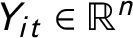$Y_{it} \in \mathbb {R}^{n}$ is the outcome response variable for observation i at time t, and $ {X}_{it}$ is an $n \times p$ matrix of p predictors at time t. In many cases, the goal is to estimate the relationship between $Y_{it}$ and $ {X}_{it}$ . For a varying-coefficient generalized linear model (Hastie and Tibshirani Reference Hastie and Tibshirani1993), one does this by treating $Y_{it}$ as a random variable whose mean $\mu _{it}$ relates to the predictors $ {X}_{it}$ as follows:

(1) $$ \begin{align} g(\mu_{it}) = {X}_{it} \boldsymbol{\beta}_{t}, \hskip 1pc i = 1, \ldots, N \hskip 1pc t = 1, \ldots, T. \end{align} $$

where a separate vector of p coefficients, $ {\beta }_{t} = (\beta _{1t}, \beta _{2t}, ..., \beta _{pt})$ , is fit for each time period and $g(\cdot )$ is an appropriately chosen link function that maps $\mu _{it}$ to a linear function of the predictors $ {X}_{it}$ . Common choices of $g(\cdot )$ include the identity, logit, and natural log function, corresponding to multivariate linear, logistic, and Poisson regression, respectively.Footnote ⁴

In the case of a pooled glm, one is quantifying the average effect of $ {X}_{it}$ on the mean of $Y_{it}$ , requiring a static relationship between $ {X}_{it}$ and $Y_{it}$ through time. The average relationship is accurate across each time period and equivalent to a time-varying model if $ {\hat {\beta }}_{1} = {\hat {\beta }}_{2} = \cdots = {\hat {\beta }}_{T}$ . For many applications this assumption simply does not hold, as the relationship between $ {X}_{it}$ and $Y_{it}$ is dynamic for at least one key variable.Footnote ⁵ In light of such concerns over detecting where relationships change and understanding why, we provide a technique that answers two questions about the relationship between two variables:

1. 1. Is the effect $ {\beta _{t}}$ constant through time?

2. 2. If $ {\beta _{t}}$ is not constant across all time points, then when does the effect significantly differ from previous periods?

2.1 Detecting Change Locations

Consider a time series of coefficient estimates for a generalized linear model in Equation (1):

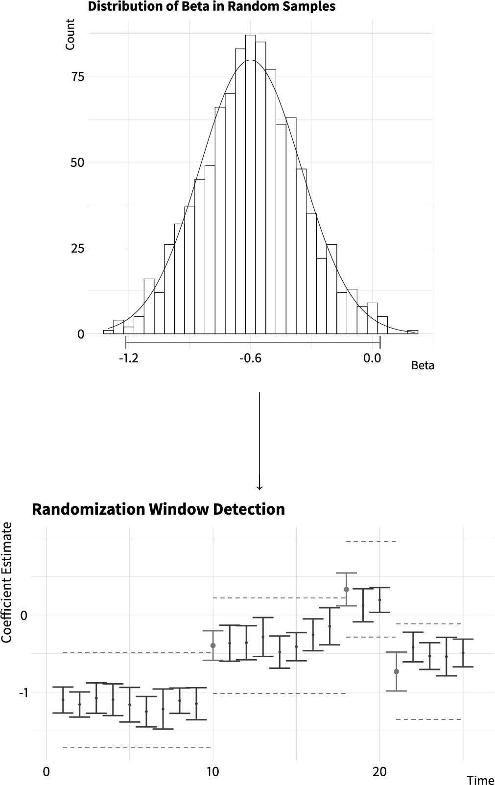
$( {\hat {\beta }}_{1}, \, {\hat {\beta }}_{2}, \, \ldots , \, {\hat {\beta }}_{T})$ . If the relationship is constant across any period of time, then each observed $ {\hat {\beta }}_{t}$ estimate within that range will vary around a stable mean value. However, if the relationship changes, then the subsequent observed $ {\hat {\beta }}_{t}$ estimates will vary around a new value. For any two variables, a visual demonstration of such a time-varying relationship can be found at the bottom of Figure 1. Detecting changepoints in such a time series is a statistical challenge because predictions are unverifiable and all time points are candidates for change, meaning there are an unknown number of partitions in the time series with unknown locations. In this sense, one is faced with an unsupervised exercise of estimating $\text {Pr}(\text {Change}_{t} = 1)$ for each point in time.

Figure 1

Display of constructing and applying the moving window. The top distribution includes the estimated values of $\hat {\beta }$ from random temporal samples. The blue bar at the base of the distribution is the estimated tolerance region, $\mathcal {R}$ . The lower figure then is the time series of coefficient estimates for the simulated data. The tolerance region begins at time = 1 and once a coefficient’s point-estimate falls outside of the region a change is signaled. That change is colored blue. A new region is built around the change with the same size but a new center.

In order to detect where changes have occurred, we draw on the SPM literature and apply a moving window to the time series of coefficients $ {\hat {\beta }_{t}}$ . SPM approaches take a statistic ${S}_{t}$ (in our application coefficient estimates), or more generally a vector of statistics $\boldsymbol {S}_{t}$ , that provides a summary of a dataset $\{( {X}_{t}, Y_{t}),~ t = 1, \ldots , T\}$ . Perhaps the most common SPM approach for identifying multiple changes is a moving-window control chart (Ge et al. Reference Ge, Song and Gao2013). In a typical moving-window approach, one produces a tolerance region, $\mathcal {R}$ , based upon the values of $S_{t}$ in a training period. For each new set of observations $({X}_{t}, Y_{t}$ ), $S_{t}$ is calculated. The new data is deemed “typical” if $S_{t} \in \mathcal {R}$ and deemed “anomalous” otherwise. Once a data point is labelled anomalous, a new tolerance region is produced.

Our approach determines the size of $\mathcal {R}$ through permutation inference before monitoring the time series. By repeatedly sampling a random set of time periods without replacement, extracting all data in those time points, and estimating the coefficient of interest, we are able to approximate a null distribution of time-invariant coefficients. Because the time periods are sampled at random, any observed differences across estimates are not expected to be due to the time periods selected. The permutation-based null distribution informs the tolerance region’s size by estimating how much coefficient variation occurs when the relationship is time-invariant. More formally, this permutation procedure is executed in the following steps.

Let $Y_{it} = g^{-1}( {X_{it}} {\beta }_{t}) + \varepsilon _{it}$ , where $i = 1, ..., N$ and $t = 1, ..., T$ . Moreover, let L represent the number of sampling iterations and J be the size of each random sample, where a sample is a set of time periods. The following four steps are repeatedly carried out:

Constructing a Null Distribution for $\widehat { {\beta }}$

• • For each $\ell \in \{1, ..., L\}:$

  • – Randomly sample J time periods without replacement, so that each $j \in \{1, ..., T\}$

  • – For each $ j \in \{1,..., J\}$ extract $( {X}_{j}, Y_{j})$

  • – Estimate $\hat {\beta }$ , where $Y_{ij} = g^{-1}( {X}_{ij} {\beta }) + \varepsilon _{ij}$

  • – Store $ {\hat {\beta }^{(\ell )}} = {\hat {\beta }}$

The sampled values $\{\hat {\beta }^{(\ell )}: \ell = 1, \ldots , L\}$ serve as a reference distribution against which we test for change. Specifically, we construct the tolerance region $\mathcal {R}$ using a Shewhart control chart, where the tolerance region for element $\beta _{kt}$ at time t is $\hat {\beta }_{kt} \pm 3 \sigma _{k}$ , $k = 1,...,p$ where $\sigma _{k}$ is the standard deviation of the estimated coefficients $\{\hat {\beta }^{(1)}_{k}, \ldots , \hat {\beta }_{k}^{(L)}\}$ , and t is the first time point in the tolerance region. We note that the Shewhart chart is one of many possible choices of a control chart from the SPM literature. For slow cumulative changes or small changes in the observed sequence, one may instead utilize the cumulative sum or exponentially weighted moving average control charts (see Woodall and Montgomery Reference Woodall and Montgomery1999 for an overview of other possible methods).Footnote ⁶ We subsequently refer to our technique as a Shewhart chart.

For parsimony, assume that the subsequent monitoring procedure is carried out on a single variable, whose estimated coefficient at time t is $\hat {\beta }_{t}$ .Footnote ⁷ Next, a prespecified probability cutoff, $\rho $ (0.5 by default), is selected to represent the necessary probability for $\hat {\beta }_{t}$ to signal a change. The probability that $\hat {\beta }_{t}$ signals a change is then the percent of the estimated sampling distribution that is greater than or less than $\mathcal {R}$ , depending on whether the point estimate is above or below the mean value within $\mathcal {R}$ . In other words, the probability of change for each time point, Pr $\,(\text {Change}_{t} = 1)$ , is the density of the estimated sampling distribution for $\hat {\beta }_{t}$ outside of $\mathcal {R}$ . Though easily changed, as a default if a coefficient’s point estimate is not inside $\mathcal {R}$ , then we reflect most SPM approaches and label an estimate as a change because more than half of the sampling distribution is outside $\mathcal {R}$ . This follows standard practice with logistic regression, where a predicted probability greater than 0.50 is generally classified as 1, rather than 0, because 1 is more likely than not. If the estimated $\text {Pr}\,(\text {Change}_{t} = 1)> \rho $ , then $\hat {\beta }_{t}$ is labelled a changepoint. Formally, this process is carried out as:

Monitoring a Coefficient, $\hat {\beta }_{t}$

• • For each $t \in \{1, ..., T\}$ , with a prespecified threshold $\rho $ :

  • – If $t = 1$ :

    • * Let $\mu _{k} = \hat {\beta }_{t}$ , where $k \in \{1, ..., K\}$ and K is the final number of partitions.

    • * Let $\mathcal {R}_{k} = \mu _{k} \pm 3\sigma $ , where $\mathcal {R}_{k}$ is the tolerance region for partition k and $\sigma $ is the standard deviation of the estimated null distribution of time-invariant effects.

  • – Else:

    • * If: Pr $\,(\hat {\beta }_{t} \in \mathcal {R}) \leq \rho $ , where Pr $\,(\hat {\beta }_{t} \in \mathcal {R})$ is the percent of the sampling distribution for $\hat {\beta }_{t}$ within $\mathcal {R}$ :

      • ⋅ $\hat {\beta }_{t}$ is not labelled a changepoint and Pr $\,(\hat {\beta }_{t} \in \mathcal {R})$ is stored.

    • * Else:

      • _⋅ $\hat {\beta }_{t}$ is labelled a changepoint and Pr $\,(\hat {\beta }_{t} \in \mathcal {R})$ is stored.

      • ⋅ A new tolerance region, $\mathcal {R}_{k}$ is calculated, where $\mathcal {R}_{k} = \hat {\beta }_{t} \pm 3\sigma $ .

2.2 Minimizing Overfitting

Given the range of options for changepoint analysis (Aminikhanghahi and Cook Reference Aminikhanghahi and Cook2017), why is the proposed technique favorable? The method’s conceptual strength stems from its ability to avoid overfitting. As discussed in Haynes, Eckley, and Fearnhead (Reference Haynes, Eckley and Fearnhead2017) and Killick and Eckley (Reference Killick and Eckley2014), changepoint analyses are easily susceptible to mistaking noisy fluctuations for genuine change, inspiring a literature on penalties meant to offset this risk.Footnote ⁸ For example, in a popular R package, estimates are produced by minimizing the following: Footnote ⁹

(2) $$ \begin{align} \sum_{i=1}^{m+1}\left[\mathcal{C}(y_{(\tau_{i-1} + 1):\tau_{i}})\right] + \beta f(m). \end{align} $$

Here m is the number of proposed partitions, y is the ordered data sequence, $\tau _{i-1}$ and $\tau _{i}$ are the start and end of candidate partitions, $\mathcal {C}$ is a cost function, and $\beta f(m)$ is a penalty that guards against overfitting. For example, the penalty value we use in simulation with this software is $2\times \text {log}(n)$ , which is equivalent to the BIC/SIC penalty. In general, $\beta f(m)$ is a tunable parameter which dictates the number of changepoints identified.

The emphasis placed on penalty inclusion in popular research and software captures the challenge posed by overfitting. However, in these applications, because true changepoints are unknown one cannot evaluate the quality of their exogenously set penalty. This leaves the researcher without knowledge of whether or not they are applying a penalty that is too strict or too light. We sidestep this tuning problem altogether through the permutation-based null distribution, which lets the data inform a threshold for differentiating noise from actual change.

3 Simulation Results

In order to test our method’s performance we conduct a Monte Carlo simulation, evaluating the Shewhart chart’s performance at each iteration and comparing it to alternative methods for changepoint analysis.Footnote ¹⁰ When evaluating the Shewhart chart across iterations, we compare it to BCP analysis (Erdman and Emerson Reference Erdman and Emerson2007), the non-BCP techniques referenced in Equation (2), and a cumulative sum control chart (CUSUM) test. These alternative methods and accompanying R packages are chosen because they cover most approaches to changepoint analysis, have reasonable runtimes, and do not require that the user prespecifies the number of changepoints.Footnote ¹¹

The steps of each simulation iteration were specified so that data for a varying-coefficient linear model, $Y_{it} = X_{it} {\beta }_{t} + \varepsilon _{it}$ , was generated with a prespecified number of changes in $\beta _{t}$ for one predictor, $x_{1t}$ , with all other relationships constant across the data. For each iteration a regression for every time period was fit, all methods were applied to estimates for the time-varying coefficient, and the difference between the true and estimated number of changes was stored. Across iterations, $\sigma $ (the standard deviation for the distribution which coefficients were drawn from) was varied in magnitude when the time-varying coefficient $\beta _{t}$ was generated, manipulating noise within each stable portion of time series. Specifically:

Monte Carlo Simulation Steps

• • For each iteration:

  • – The number of changepoints, P, is drawn from a truncated normal distribution.Footnote ¹²

  • – The location(s) of parameter changes are determined through P draws from a discrete uniform distribution, $U(1,T)$ .

  • – The mean value for each partition, $\mu _{p}$ , is drawn from a standard normal distribution, for $p = \{1, \ldots , P+1\}$ .

  • – Data for each time period, t is generated through a linear model where each coefficient value for the time-varying coefficient $\beta _{t}$ is drawn from a normal distribution with mean $\mu _{p}$ and standard deviation $\sigma $ .

  • – All changepoint techniques are applied to the time series of coefficient estimates $\hat {\beta }_{t}$ for the time-varying relationship.

  • – The difference between the actual and estimated number of changes is recorded.

Table 1

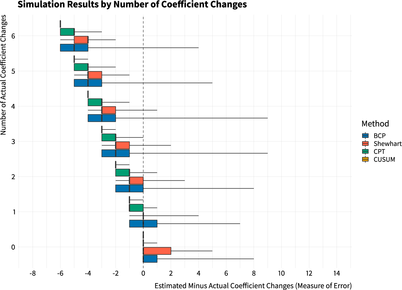
Root mean squared error by number of changes.

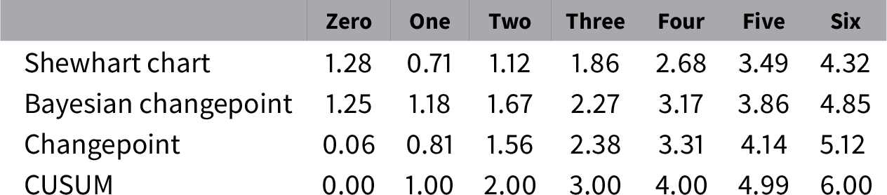
Table 1 provides a broad summary of the simulation’s results, where iterations are compared by the true number of coefficient changes. For each iteration, a method’s error is calculated as the difference between the estimated and true number of changes, meaning errors closer to 0 represent better performance. For example, if there are two changes but only one is detected, then the error would be $-$ 1. Across each number of changes, with the time series growing increasingly dynamic as the number increases, the Shewhart chart has the lowest mean squared error, except for when there are zero changes.Footnote ¹³ Though, and we return to this before concluding, the more dynamic the time-series, then, regardless of method chosen, the more difficult accurate estimation becomes.

Figure 2

Simulation results for each method stratified by the true number of coefficient changes. The x-axis corresponds to the difference between the estimated and actual number of coefficient changes. The y-axis is the true number of coefficient changes in the simulated data. The boxplots capture the summary statistics for each method’s performance. Results from BCP analysis are in blue, the Shewhart chart’s results are in red, changepoint is in green, and CUSUM in gold. Whiskers are generally one-sided because each method only tends to have especially large errors when they overfit and mistake noise for changepoints, leading to a large positive difference between the estimated and true number of changes.

Moving to a visual representation, Figure 2 displays a summary of each method’s performance across the simulation. Bayesian changepoint (BCP) analysis, which does not include a penalty, has the greatest tendency to overfit, with cases where the maximum number of errors is systematically far greater than 0. In cases where the error term is positive, the method of interest returns multiple false positives—detecting changepoints that do not exist. Considering the other methods, CUSUM tests are overly conservative and as the number of changepoints increases, the more they tend to treat the time series as having a stable mean but high variance. Changepoint analyses with an imposed penalty term avoid overfitting, having few instances of positive errors. But, the penalty appears to impose systematically too strict of a standard, rendering errors further from 0 in all cases except for those without any changepoints. Conversely, the Shewhart chart’s performance is closest to 0 across most conditions.

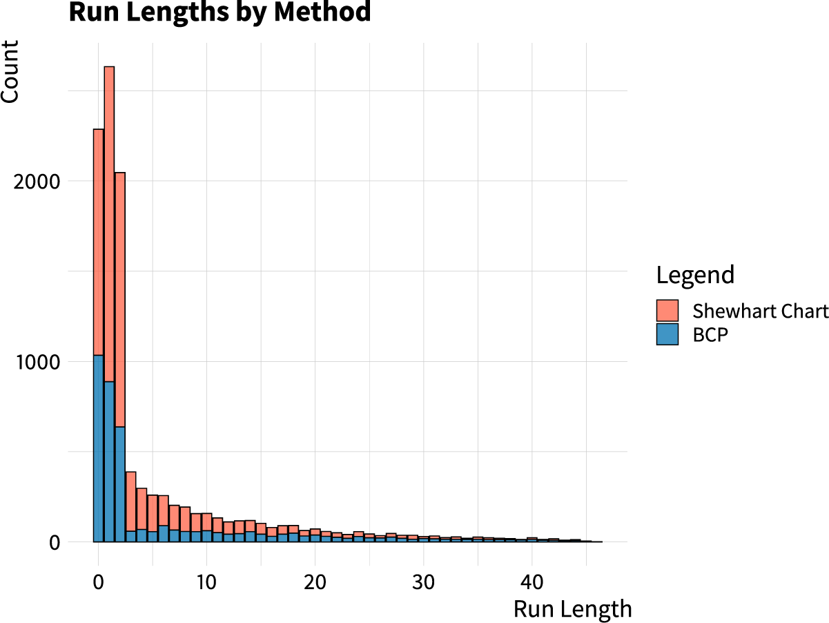
Last, we assess the average run length—the average time it takes for a change to be detected, once it has occurred. To estimate this, we ran a Monte Carlo simulation where only one change occurs, but the magnitude of this change and its location varies. We then applied all techniques to the resulting time series of coefficient estimates, recording whether a change was detected and, if detected, the time elapsed after the change until detection. We present the results of the simulation in Figure 3 and Table 2. CUSUM and non-BCP tests are left out of these descriptive statistics because they tend to fail to detect a change in these situations. Visually, the results look similar across techniques. A closer look at the summary statistics reveals a more nuanced story, however. While the two methods perform similarly when a change is detected, with a lower mean for the Shewhart Chart but an equivalent median for both, the false-negative rate (undetected changes) is far higher for BCP analysis. Because there are so many more undetected changes for the Bayesian approach, its bars in Figure 3 are shorter than those for the Shewhart chart.

Figure 3

Distribution of run lengths for each method in a Monte Carlo simulation where only one change occurs. CUSUM and non-BCP results are not included because the methods tend to be too conservative and miss the change altogether. Results from the Shewhart chart are in red and BCP in blue. Run length is the amount of time between when a change occurs and the change is detected. 10,000 iterations were run in total. Cases where no change is detected are not included but noted in Table 2.

Table 2

Summary statistics for simulations with one change. The statistics represent: whether a change was detected and, if detected, the amount of time after a change before it is detected.

4 Application to Militarized Interstate Disputes

To demonstrate the model’s applicability, we replicated Leeds’ (Reference Leeds2003) study on the relationship between alliance types and the initiation of militarized interstate disputes (MIDs). Using data spanning from 1816 to 1944, Leeds fits a generalized estimating equation (Zorn Reference Zorn2001) with terms for the association between various types of alliances—defensive alliances, offensive alliances, and neutrality pacts—and the initiation of a MID. Leeds argues that defensive alliances are negatively associated with MID initiation and that offensive alliances and neutrality pacts are positively associated with MID initiation. The results are important because they establish the actual empirical association between these variables, whereas theoretically relationships in varying directions are plausible. Moreover, applying the Shewhart chart introduces the question: “Under what conditions are alliances more versus less effective deterrents?,” rather than solely focusing on whether alliances appear effective on average.

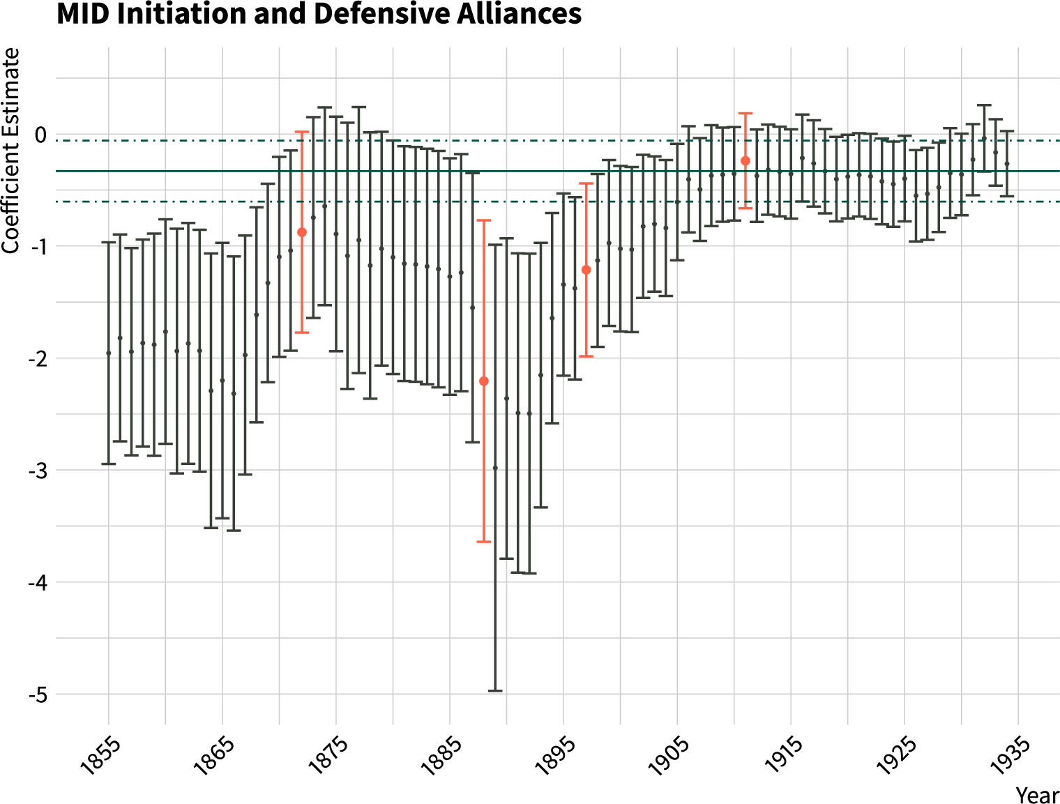
In order to test for the number of changes and their location, we obtained coefficient estimates over time by fitting a varying-coefficient model across temporal subsets of the dataset. Specifically, we produced estimates by: selecting twenty years of data,Footnote ¹⁴ fitting the model, storing results, moving forward one year, fitting the model again, and so on.Footnote ¹⁵ This approach allowed us to maximize the number of coefficient estimates while ensuring each model included sufficient data.Footnote ¹⁶ The results can be seen in Figure 4. First, as a reference point for the previously unmodeled heterogeneity, the pooled model’s point-estimate and confidence interval are included across the figure in green with dot-dashed lines for confidence intervals. Next, coefficient estimates which are not detected as a change are included in black and detected changes by the Shewhart chart are in red with larger dots. The estimates which are predicted to be changepoints include data from 1862 to 1882, 1878 to 1898, 1897 to 1907, and 1901 to 1921. It then follows to ask why these time periods correspond with estimated changes, whereas others do not. A full investigation of the substantive sources of these changepoints—and why other time periods are not changes—is beyond the scope of this manuscript. The first two changepoints, however, lend credence to the impact of the Wars of German Unification and then the loss of Bismarck’s leadership. The final two changepoints are likely indicative of the move toward World War I and then its start.

Figure 4

Replication and extension of Leeds (2003). Red, larger estimates correspond to changes detected by the Shewhart chart. Black estimates are considered stable by both techniques. The pooled model’s results are a reference point across the figure in green, with dot-dash lines for the pooled confidence interval.

Lastly, considering the missed variation that follows from a pooled model, during the long peace associated with the Concert of Europe defensive alliances were associated with far greater deterrent effects than the pooled model finds. This relationship dissipates and almost disappears with WWI, the interwar period, and WWII.Footnote ¹⁷ This suggests that the pooled estimate is actually somewhat conservative for much of the data.

5 Discussion and Conclusion

We develop a statistical procedure for detecting the locations of coefficient changepoints when fitting generalized linear models to TSCS data. The technique first estimates the bounds for stable statistical behavior through a permutation procedure, which then determines the size of a Shewhart chart that returns the probability of effects changing at each point in time. In a Monte Carlo simulation we find that this procedure outperforms BCP analysis, non-BCP analysis, and CUSUM tests in most simulated conditions. Last, we apply our techniques to a popular study on the relationship between alliances and the onset of conflict, revealing substantial unmodeled effect heterogeneity.

Before concluding, two cautionary points are merited. First, as Table 1 and Figure 2 demonstrate, as the number of changepoints increase in simulation iterations, the more inaccurate all methods become. Given that the exercise is unsupervised, it is not necessarily surprising that all methods struggle with these hard cases. But the results do suggest that one should consider how dynamic the time series of interest appears to be before making strong claims about detected changepoints. If the time series is highly dynamic, then, regardless of method, detecting all changepoints is a substantial statistical challenge. In such a case, one may be better suited investigating the accuracy of their coefficient estimates, exploring potential unmodeled confounders, and more.

Second, while the proposed technique and R packageFootnote ¹⁸ are readily extendable to other statistics of interest that occur over time, one needs the underlying data to apply our technique. More specifically, the null distribution of time-invariant effects can only be estimated if the data $( {X}_{it}, Y_{it})$ is available for each randomly selected set of time points. If one solely has access to a time series but none of the data used to generate that time series, then our method cannot be applied. In this case, other methods must be considered.

Although unmodeled effect heterogeneity poses the risk of faulty pooled inferences, it also presents an opportunity to theorize the sources of temporal effect variation. Why might effects change at one time and not another? Why might one change in effects be larger than others? These types of questions are substantively interesting and valuable. However, before these questions can be asked one must differentiate stable variation from genuine changes, which is a statistical challenge. Our proposed technique provides a straightforward means of doing so and improves upon existing approaches.