Introduction
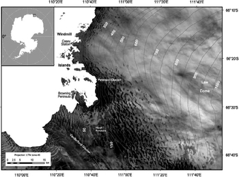
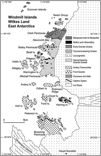
The Windmill Islands are a group of topographically low (<100 m) islands and peninsulas situated on the western margin of the Law Dome ice cap, East Antarctica, at approximately 66°20'S, 110°30'E (see Fig. 1). Roughly circular in shape and with a maximum elevation of approximately 1400 m, Law Dome is known to have extended well over the top of the Windmill Islands area during the Last Glacial Maximum, but has since retreated to expose the islands (Cameron Reference Cameron1964, Goodwin Reference Goodwin1993, Goodwin & Zweck Reference Goodwin and Zweck2000). This group of islands is important to the study of subsurface geology and post-glacial isostatic processes in the region as it is the only extensive stretch of exposed land, i.e. free of ice, for 400 km in any direction. Understanding the gravity response of local geology will contribute to ongoing interpretation of regional-scale gravity surveys such as ICECAP. As well, understanding the geometry and geology of the bed of the Law Dome will aid in interpreting origins of jökulhlaups and their implications for water beneath Antarctica. Figure 2 shows the Windmill Islands, which consist of 75 km2 of discontinuously exposed bedrock over an area of approximately 450 km2 (Cameron Reference Cameron1964).
The Windmill Islands on the western edge of the Law Dome ice cap, East Antarctica. Topographical heights are in metres, 50 m contour lines. (Map adapted from the Casey ice runway map provided by the Australian Antarctic Data Centre.)

The Windmill Islands showing prominent locations and rock units (adapted from Paul et al. Reference Paul, Stuwe, Teasdale and Worley1995). A–A’ is the location of the gravity profile in Fig. 5.

The aim of the study was to supplement the existing gravity network and to investigate the subsurface geology of the Windmill Islands region using the gravimetric method. The geophysics of this region has received little attention, with only two gravity surveys conducted previously. The first was in 1962 (Walker Reference Walker1966, Reference Walker1976) while the second was in 1993–94 (Haydon Reference Haydon1994). No previous attempts using any technique have been made to produce a model of the subsurface geology. The data in this paper (142 gravity stations over approximately 450 km2) are the union of the 1993–94 and 2004–05 season surveys, with the 1962 season survey being effectively resampled. This combined dataset enabled a Bouguer anomaly map and a 3D subsurface model to be constructed of the central area of the Windmill Islands region where gravity station concentration is highest.
Geological setting
The Windmill Islands (Fig. 2) consist of a layered sequence of schists, gneisses and migmatites (the Windmill Metamorphics) intruded by a porphyritic granite (the Ford Granite) and a charnockite unit (the Ardery Charnockite), which are cut by two swarms of easterly trending gabbro dykes (Blight & Oliver Reference Blight and Oliver1977, Reference Blight and Oliver1982, Post et al. Reference Post, Henson and Kinny1997). Early geological mapping and dating of the Windmill Islands rock units began in 1956 (Ravich & Voronov Reference Ravich and Voronov1958), and was followed by Cameron et al. (Reference Cameron, Goldich and Hottman1960), Cameron (Reference Cameron1964), Webb et al. (Reference Webb, McDougall and Cooper1964) and McLeod & Gregory (Reference McLeod and Gregory1966). Since then, the rocks of the Windmill Islands have been extensively studied by Blight & Oliver (Reference Blight and Oliver1977, Reference Blight and Oliver1982), Williams et al. (Reference Williams, Compston, Collerson and Arriens1983), Paul et al. (Reference Paul, Stuwe, Teasdale and Worley1995), Post et al. (Reference Post, Henson and Kinny1997) and Zhang et al. (Reference Zhang, Zhao, Liu, Liu, Hou, Li and Ye2012). The metamorphic grade of the Windmill Metamorphics ranges from upper amphibolite facies (sillimanite-biotite-orthoclase) in the north, through biotite-cordierite-almadine granulite to hornblende-orthopyroxene-granulite in the south (Blight & Oliver Reference Blight and Oliver1982). The structural and metamorphic relationships in the Windmill Islands geology show evidence for repeated tectonothermal activity (Paul et al. Reference Paul, Stuwe, Teasdale and Worley1995), with four distinct deformation episodes having been identified by Blight & Oliver (Reference Blight and Oliver1977, Reference Blight and Oliver1982).
Using SHRIMP (Sensitive High Resolution Ion MicroProbe) U-Pb zircon dating, Post et al. (Reference Post, Henson and Kinny1997) calculated the age of deposition of the Windmill Islands metasediments to be 2500–1700 Ma. This was followed by the four, undated, distinct deformation episodes first identified by Blight & Oliver (Reference Blight and Oliver1977, Reference Blight and Oliver1982) and further documented by Post et al. (Reference Post, Henson and Kinny1997), Post (Reference Post2000) and Zhang et al. (Reference Zhang, Zhao, Liu, Liu, Hou, Li and Ye2012). Using Zircon LA-ICP-MS U-Pb geochronology Zhang et al. (Reference Zhang, Zhao, Liu, Liu, Hou, Li and Ye2012) date the Garnet-bearing Granite Gneiss at 1250 Ma. Zhang et al. (Reference Zhang, Zhao, Liu, Liu, Hou, Li and Ye2012) date the Ardery Charnockite at 1200 Ma, while Post et al. (Reference Post, Henson and Kinny1997) report an age of 1160 Ma suggesting a long period for its emplacement. The Ford Granite was emplaced at 1170 Ma following the second deformation event (Post et al. Reference Post, Henson and Kinny1997).
Survey procedures, fieldwork and method of analysis
During 2004–05, two Lacoste and Romberg gravity meters, G104 and G101, were used to measure gravity at 97 stations. The survey was primarily carried out using inflatable rescue boats for transport, and therefore, the majority of the gravity measurements were taken near the boat landing sites close to sea level. Only meter G104 was used during this activity. Hagglunds (tracked vehicles) were the main mode of transport for surveying the peninsulas. Position and gravity observations were generally taken at local high points, often old survey stations due to their ease of subsequent re-identification and reoccupation. Both G104 and G101 were used in this segment. Finally, where the islands were enclosed by sea ice and joined to the mainland in the area surrounding Browning Peninsula, man hauling and backpacking with only G104 was undertaken.
Due to logistical constraints, two handheld Garmin GPS units were used for positioning at each gravity station. These constraints included the weight of equipment, transportation distance, distance from continuously operating base stations and station occupation time. These handheld GPS receivers applied the EGM96 geoid separation model (Lemoine et al. Reference Lemoine, Kenyon, Factor, Trimmer, Pavlis, Chinn, Cox, Klosko, Luthcke, Torrence, Wang, Williamson, Pavlis, Rapp and Olson1998) to convert ellipsoidal heights to orthometric heights. No transformations were applied to the longitudes and latitudes, which were recorded in the WGS84 reference frame. Additionally, both receivers were calibrated over two levelled tide gauge benchmarks on three independent sessions (Morgan Reference Morgan2011). These three sessions ensured that different GPS satellite geometries and conditions were sampled; thereby providing a local correction to the EGM96 model so that heights were relative to mean sea level. The precision of the mean height from both receivers is estimated using variance propagation to be ±2.7 m, 1-sigma (Morgan Reference Morgan2011). Horizontal positions have a precision better than ±2 m, 1-sigma, in each component.
The small 1993–94, 49 station gravity dataset of Haydon (Reference Haydon1994), was acquired using helicopters as the primary mode of transport. Gravity observations were taken with Lacoste and Romberg meter G398 mainly on hill tops at survey stations which provided position and elevation relative to mean sea level. Four of these stations, including station 6842.0004 (gravity mark naming convention), the adopted base station and the working base station, B5, were reoccupied on multiple occasions during the 2004–05 season and were used to tie together the two surveys. The still smaller 27 station dataset of Walker (Reference Walker1966, Reference Walker1976) has been excluded, primarily as new data was collected at 22 of these locations.
The reduction of this data was achieved in a two-step process. Step 1 was the determination of a new epoch value of the Casey mark 6842.0001. This was achieved through a least-squares adjustment of all G104 and G101 data including pre- and post-2004–05 Antarctic field season data obtained over absolute gravity stations in Hobart (Mount Pleasant and Mount Nelson Vault) and Canberra (Geoscience Australia). This solution used a single drift and scale for each meter, and resulted in the 2004–05 epoch value being determined as 982382.69 mgal (1 mgal=10 μm s-2). This adopted value is marginally higher than the Wellman (Reference Wellman1976) value of 982382.66 mgal. There are several plausible reasons for this small difference including observation and reduction uncertainties, meter calibration and consistency in reference frames. The difference is mathematically minimized in the analysis work undertaken in this paper when a third-order polynomial (approximately the regional field) is removed, since this polynomial contains a constant offset term. This base station was transferred on multiple occasions throughout the season to mark 6842.0003 (the more fundamental base station at Wilkes established by Sparkman in 1957 (Thiel et al. Reference Thiel, Bentley, Ostenso and Behrendt1959)), and two marks 6842.0002 and 6842.0004. Additionally new, more readily accessible and preservable marks at the Casey Science Building (200490.0005) and the Emergency Vehicle Shelter (200490.0006) were established.
Step 2 involved combining data from G104 and G101 with the data taken with G398 in 1993–94. In this solution the base station 6842.0001 was constrained with an uncertainty of 0.006 mgal which essentially tied the Windmill Island data to the Step 1 value of mark 6842.001 while utilizing a single whole of season drift rate and scale factor. There were four common gravity stations between the 2004–05 and 1993–94 surveys. The resultant, 1-sigma, uncertainty of a gravity observation from the combined solution was ±0.04 mgal. The gravity reference system of this solution is consistent with the current Australian gravity datum, ISOGAL84 (Wellman et al. Reference Wellman, Barlow and Murray1985), as the Canberra and Hobart gravity stations used to determine instrument scale factors and drift rates for the data are in this reference system. ISOGAL84 is consistent with IGSN71 (the International Gravity Standardisation Net; Morelli et al. Reference Morelli, Honkasalo, McConnel, Tanner, Szabo, Uotilla and Whalen1974). It is to be noted that the early record of Walker (Reference Walker1966, Reference Walker1976) is in the Potsdam 1930 system (Morelli et al. Reference Morelli, Honkasalo, McConnel, Tanner, Szabo, Uotilla and Whalen1974). The 1980 International Gravity Formula was used to compute the normal gravity field and the free-air correction using the latitude dependent reduction to mean sea level (Li & Gotze Reference Li and Gotze2001).
The ±2.7 m elevation uncertainty is the largest error source in the gravity reductions, clearly adding uncertainty to the free-air and Bouguer corrections but error sources also occur with: i) the reduction of gravity meter dial readings to milligals, ii) the average density of rock in the intervening layer between the gravity station and the reduction level (mean sea level) is imperfectly known, and iii) a component due to uncertainty associated with topographical corrections. After correcting for near-field effects, this component is estimated, through an analysis of the gravitational effect due to parallelepidides as used by Geldart et al. (Reference Geldart, Gill and Sharma1966), to be ±0.3 mgal at the 1-sigma level. The majority of this component is due to errors associated with steep cliffs. The total of these components is estimated to be ±1.16 mgal at the 1-sigma level.
The computation of above sea level near-field terrain corrections was based on the classical cylinder segment approach (see, for example, equation 2.26 or 2.58 of Telford et al. Reference Telford, Geldart and Sheriff1990). The available digital elevation model (DEM) was constructed from the Windmill Islands 1:50 000 map (Australian Antarctic Division 1997) with a tile size of 10 mx10 m by the Mapping Branch of the Australian Antarctic Division. Elevations were estimated to the 1 m level for the topography only. Mean sea level was implicitly defined by absent tiles. A local set of concentric circles were constructed for each gravity station with an incremental radius of 10 m and a centre of cell arc of approximately 10 m. This was due to the need to have an integer number of cells in each annuli. All cells were given a nominal zero elevation. This nominal elevation model was then updated using polar co-ordinates for all DEM tiles within 2 km of the gravity station. Finally, the terrain correction was computed after summing the component due to material above the station whose density was assumed to be 2670 kgm-3 and the component due to a lack of material below the station with the same 2670 kg m-3 density contrast. The number of contributing cells for validation were also tallied. This was, by design, one cell short as we also assumed that the gravity station was on flat ground out to a radius of 5 m to avoid computational instability. This computation of near-field, above sea level terrain corrections has been applied to the dataset; however, there is no bathymetric data available except in Newcombe Bay off Bailey Peninsula along the resupply route to Casey Station (a very minor portion of the total bathymetry of the survey area). Thus the detailed application of bathymetric terrain corrections cannot be undertaken with any confidence of improving the inherent uncertainty associated with station Bouguer anomalies. An analysis of near-field bathymetric terrain components (i.e. the terrain effects of bay areas within and surrounding the islands) has been conducted to examine the effects of the unapplied bathymetric terrain corrections within the Windmill Island survey. The 1-sigma uncertainty from uncompensated near-field bathymetric terrain effects are estimated to be most likely no larger than ±0.7 mgal which corresponds to a uniform slab of sea water of 10.2 m.
As terrain corrections due to far-field regional gravity effects have not been applied to these data, an analysis was needed to assess the resulting implications for the dataset. Not applying far-field terrain corrections probably leaves the Bouguer field with regional trends in both the east–west and north–south directions. Distant relief effects as a result of the ocean in the north and west, the Law Dome ice cap in the east, and the East Antarctic Ice Sheet and the deep trench associated with the Vanderford Glacier in the south must all be taken into account when considering applying far-field terrain corrections. For relief above and below each gravity station, the terrain correction must be subtracted from the conventional Bouguer contribution (Hammer Reference Hammer1939) or added to the station observed gravity (Telford et al. Reference Telford, Geldart and Sheriff1990). Mikuska et al. (Reference Mikuska, Pasteka and Marusiak2006) recommend separate treatments for the above and below sea level components.
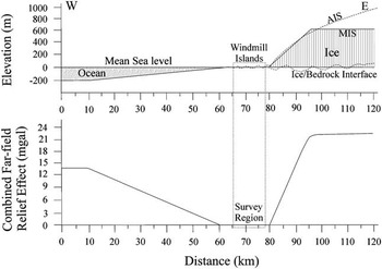
An analysis was conducted to deduce the magnitude of the gravitational effect of the sloping continental shelf to the west and the Law Dome ice cap to the east on the gravity station sites in the central region of the study area. The gravitational effects of a sloping continental shelf (200 m depth in 50 km) and the rising Law Dome ice cap (800 m height in 20 km) were investigated for a hypothetical west–east line (Fig. 3). The approach of Geldart et al. (Reference Geldart, Gill and Sharma1966), which uses sloping faults, was utilized. This shows that, providing the stations under investigation are greater than 2 km away from the far-field source, there would be little to no contribution of either the sloping continental shelf or the rising Law Dome ice cap to the majority of our gravity stations. Our analysis indicates that the combined far-field contribution of the continental slope and the Law Dome ice cap is less than 0.3 mgal and can be neglected as the stations are well removed from these features. The ice filled Totten-Vanderford Trench to the south is different in that this feature is extensive with steep and abrupt changes in surface slope, and hence, is likely to have a more significant effect over the Windmill Islands. We have chosen to neglect the effect, primarily due to large horizontal distances to it apart from the two southern most stations around Haupt Nunataks and the fact that a slowly decaying signal can be modelled with low-order polynomial surfaces.
Modelled far-field terrain effects on the Windmill Islands contributed by the ocean in the west and the Law Dome ice cap in the east. Model parameters used: the ocean floor extending from the western edge of the Windmill Islands, sloping at 0.229° to a depth of 200 m (based on Sandwell & Smith (Reference Sandwell and Smith1997) ETOPO-2 data), and an ice cap extending from the eastern edge of the Windmill Islands with an ice surface slope of 2.29° to a height of 800 m. The adopted ice/bedrock interface has been set at zero elevation (mean sea level). This is based upon ice echosounding and seismic data as reported by Pfitzner (Reference Pfitzner1980), which is shown as a dotted line undulating around zero elevation beneath the ice cap. The model ice surface (MIS) topography can be seen to be a good approximation of the actual ice surface (AIS) reported in Pfitzner (Reference Pfitzner1980). It is shown that the far-field terrain effects have little to no effect on the survey area relevant to modelling within the Windmill Islands (bounded by the dashed lines box).

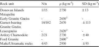
All gravity station locations were chosen to be on rock, not on ice, to enable precise reoccupation for future time series studies, and to allow more precise Bouguer corrections (the thickness of ice between the gravity stations and bedrock would create additional type (iii) uncertainties). In situ samples were collected to obtain a working a priori rock density. Where possible, an effort was made to acquire several samples from each of the main rock groups. Each of the samples was cored (25 mm diameter) and cut to length (22 mm) to obtain specimens for density analysis. From the in situ rock samples collected from the Windmill Islands, a density analysis of each rock unit was performed. From this analysis, each rock group was assigned a density range to apply constraints during 3D modelling. For certain rock units where fresh in situ samples could not be collected, densities were assigned using data from Haydon (Reference Haydon1994) and Hollin et al. (Reference Hollin, Cronk and Robertson1961). The average rock sample densities deduced through analysis and used in modelling are summarized in Table I. An area average of these values, 2670 kgm-3, has been adopted for Bouguer processing. Geosoft Oasis Montaj Version 6.1 was used to grid the Bouguer field. The software contours the gridded data using a minimum curvature algorithm.
Summary of rock densities from the Windmill Islands.
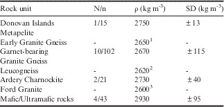
1 Adopted from Hollin et al. (Reference Hollin, Cronk and Robertson1961).
2 Adopted from Haydon (unpublished).
3 Deduced from modelling in this paper.
N/n=no. of samples/no. of measurements.
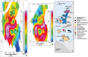
A third-order polynomial trend surface was removed from the reduced and gridded gravity dataset to remove the regional trend created by far-field gravity signals, thus enhancing the gravity signature associated with the subsurface geology. This third-order polynomial was removed from the gridded Bouguer field to produce a residual gridded Bouguer anomaly image for subsurface modelling (Fig. 4b).
Results
Bouguer anomalies
The observed Bouguer gravity field over the Windmill Islands is shown in Fig. 4a together with the locations of the gravity stations. As there is considerable uncertainty associated with the performance of estimators associated with the regional component of the gravity field at or near unconstrained edges, we limit our discussion, by involving a mask, to the central region which is shown in Fig. 4b. This inner region contains 133 gravity stations dispersed over an area of approximately 260 km2, which equates to an average area of 2.0 km2 per gravity station providing an ample dataset for subsurface modelling. An alternative view is that the average inter-station distance between gravity stations in this inner region is 0.8 km. It should be noted that there are bay areas in which no gravity stations were able to be established, and hence the concentration will be less in these areas while in other areas, notably the peninsulas and the island groups, which have a higher concentration of stations.
Bouguer gravity image of the merged 1993–94 and 2004–05 Windmill Islands gravity dataset. b. Residual Bouguer anomaly image. c. Simplified geology map of the area (adapted from Paul et al. Reference Paul, Stuwe, Teasdale and Worley1995). Correlations between the Bouguer anomalies and major geological units are evident. It can be seen that the dominant positive anomaly in the south is produced by the dense Ardery Charnockite unit, surrounding the relative low created by the Ford Granite pluton. The ice ramp can be seen as the small negative anomaly on Mitchell Peninsula at 66°20'S, 110°34'E. The Bouguer anomalies in the northern portion of the image are influenced by metamorphic rock units of varying densities, with the negative anomaly on Clark Peninsula caused by the less dense Early Granite Gneiss, and the negative anomaly offshore from Mitchell Peninsula resulting from the low density leucogneiss. The small triangles represent the 1993–94 gravity station locations, and the small black circles represent 2004–05 gravity station locations. The modelled profile line can be seen (labelled A–A’) passing through Holl, Ford and Herring islands.

The residual Bouguer image (Fig. 4b) exhibits correlations with the major rock units of the area (Fig. 4c). The dominant gravity feature on the anomaly map is the relative high that is associated with the relatively dense Ardery Charnockite unit (see Table I). This positive anomaly bends around the negative anomaly created by the less dense Ford Granite. A subtle relative low is situated just to the east of the Ford Granite pluton beneath Herring Island. There is a distinct negative anomaly centred on Clark Peninsula that correlates with the low density Early Granite Gneiss, the most common rock unit of Clark Peninsula. On the northern portion of Clark Peninsula and making up part of the Swain Group of islands is the interlayered Metapelite and Metapsammite unit, which does not appear to have a significant effect on the gravity signature. The only major leucogneiss unit of the area is situated west of Mitchell Peninsula, making up Hollin, Midgley, Pidgeon and Warrington islands. It displays a localized high amplitude negative anomaly. The relative low on Mitchell Peninsula proper that extends eastwards toward Law Dome is not consistent with Garnet-bearing Granite Gneiss but rather with a lower density material, most probably a mixture of ice and rock.
Modelling
The 3D modelling technique used in this study is called Section Modelling within the Encom software, Modelvision Pro 7.0. This technique involves dividing up the grid into east–west or north–south sections which are individually modelled before being joined to create the whole. The process is iterated and re-computed to ensure that each section fits its own unique Bouguer gravity profile as smoothly as possible, ensuring that a regional best-fit 3D model is generated. For this study, the grid was divided up into 1-km and 2-km wide, east–west oriented vertical sections. Two-kilometre wide sections were modelled in the southern and northern areas, whilst 1-km wide sections were modelled in the central area where data is denser and geological units are more complex. Maximum model depth is 15 km.
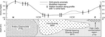
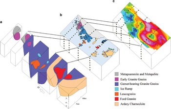
A modelled profile through the Ardery Charnockite, the Ford Granite and the Garnet-bearing Granite Gneiss along line A–A’ of Figs 2 & 4b is shown in Fig. 5. A subsurface 3D block diagram of the region derived using this modelling process is shown in Fig. 6a. A good correlation with the major geological units of the area can be seen (Fig. 6b), in particular the intrusive rock units at locations producing a relative high anomaly (dense charnockite at 2730±40 kg m-3) and an unsampled, isolated, relative low (less dense granite at 2600 kgm-3) are clearly visible. The modelled depth of the Ardery Charnockite is ~9±3 km in the northern and central regions, and ~5±2 km in the south (Fig. 6a). The 1-sigma limits of these depths have been deduced by changing the density of the charnockite to reflect its statistical variation and remodelling, whereas rigorous propagation techniques have been more generally adopted elsewhere in this work. The reliability of these depths and thicknesses was tested by varying these parameters in our model. In all cases the size of the residual between model gravity and observed gravity increased when these parameters were reduced. The western edge, over Holl Island, was very sensitive to these parameter changes. We are able to deduce the nature of the contacts using the regional model. The eastern contact has a steep dip (60–90°) and lies between Holl and Ford islands. The northern contact, north of Ardery Island, Odbert Island and Robinson Ridge, dips steeply to the north. The western contact is not discernible as there is no gravimetric or geological data. However, note that the peak of the gravity high occurs over Holl Island and gradients are relatively high. Thus, there is the expectation that the western contact is both steep and not too far to the west of Holl Island. The southern contact is also ill-defined. This work shows this contact to be south of Browning Peninsula, the effective limit of gravimetric and geological information. The indications are that the contact is steep. The model also suggests that the Ardery Charnockite is a thick, vertical, tabular body of igneous rock extending over much of the southern section of the Windmill Islands.
A modelled east–west trending profile (2 km wide section) through the Ardery Charnockite, the Garnet-bearing Granite Gneiss, and the Ford Granite, located slightly north of 66°25'S. The modelled response line is matched as closely as possible to the measured gravity line under geologically feasible constraints. It can be seen that the model is a poor fit in the region surrounding 110°35'E where there are no gravity stations as there are no islands present to allow measurements. The gridding procedure extrapolates this region to be a relative high; however, it is more likely to be a linear gradient between the two stations on either side of this bay. All densities shown are in kg m-3.

Block model of the Windmill Islands region and subsurface. a. The 3D model sliced along relevant east–west oriented transects to show the depth extents and orientations of the region’s major rock units. There is no vertical exaggeration, indicating the true dip of bodies and contacts. b. Geology map of the Windmill Islands (adapted from Paul et al. Reference Paul, Stuwe, Teasdale and Worley1995), with dotted black lines representing the slices. c. The Bouguer anomaly map of the Windmill Islands with dotted black lines representing the slices. See Fig. 4 for the associated Bouguer anomaly legend.

Discussion
The residual Bouguer image (Fig. 4b) exhibits correlations with the major rock units of the area (Fig. 4c). This image is not dissimilar to the same broad features postulated by Walker (Reference Walker1966) from his small 29 station gravity dataset. Either side of the modelled profile (Fig. 5) are extended marine areas where both gravimetric and geological data are interpolated from well-constrained data. This means that the adjacent marine profiles are less reliable, which in turn limits the reliability of the preferred model especially as we move further away from the constrained profile.
A second significant issue is the reliability of the profile to represent the subsurface geology. This reliability is also tied to station density and the adopted methodology. From Fig. 5 there is good agreement except in the middle segment where there is a significant departure between the observed and modelled values of the profile. It is immediately evident that there is a data paucity in this discrepancy region, caused by water, which limits the determined profile. It is also evident, on reviewing Fig. 4b, that the ridge which generates the local high may be a gridding artefact. Our evidence for this is two-fold: i) The ridge is not apparent when tension is applied to the minimum curvature splines (Smith & Wessel Reference Smith and Wessel1990) or when Delauney triangulation (Shewchuk Reference Shewchuk1996) is used to derive a basic Bouguer gravity field. We were unable to implement these variants within the chosen Encom software package. ii) A single granite pluton (the Ford Granite) cannot account for the anomaly pattern, yet it is most unlikely that the emplacement of this pluton would be anything other than a single pluton. It is noted that the isolated relative negative anomaly on Herring Island may be attributed to a separate granitic blind pluton; however, it is much more likely that a gridding artefact is present separating the one negative anomaly into two. The gravity is well-modelled at Ford Island in the west, and in the east, modelling of the gravity suggests that the pluton extends beneath the western portion of Herring Island at depth. It is also noted that the eastern end of the profile line in Fig. 5 has a ‘High mafic concentration region’ which has a higher density (2750 kg m-3) than the usual Garnet-bearing Granite Gneiss. This is required for the modelled response to fit the anomaly profile. This is feasible as Paul et al. (Reference Paul, Stuwe, Teasdale and Worley1995) observed approximately 70% Garnet-bearing Granite Gneiss and 30% mafics and ultramafics in this region of Herring Island. Hence a mixed rock density of 2750 kg m-3 has been used in the modelling based on the percentage of these rocks mapped on Herring Island.
The dominant gravity feature on the anomaly map is the relative high that is associated with the relatively dense Ardery Charnockite unit (Table I). Intrusive charnockites typically form during the thickening of the crystalline basement and shields when the crystallization of granite magma in the deep zone of the Earth’s crust takes place, and then the magma is emplaced as charnockitic plutons at various levels in the crust (Ravich Reference Ravich1972, Grikurov et al. Reference Grikurov, Kamenev and Kameneva1982). This results in charnockite bodies of various sizes and shapes, ranging from small dome-like plutons to larger batholith-like plutons outcropping over thousands of square kilometres (Ravich Reference Ravich1972). Grikurov et al. (Reference Grikurov, Kamenev and Kameneva1982) have noted that the largest intrusive charnockites are of tabular and lens-like shape extending to depths of several kilometres, whereas the smaller units are generally domes or stocks. To give an indication of the size of the charnockite units present in East Antarctica, the Mawson Charnockite in Mac. Robertson Land is exposed over an area of 10 000 km2 (Kizaki Reference Kizaki1972) and a large pluton, the Lodochnikov Massif charnockite, of Queen Maud Land is exposed over 4000 km2 (Ravich Reference Ravich1972, Mikhalsky et al. Reference Mikhalsky, Sheraton and Hahne2006). Finally, Grikurov et al. (Reference Grikurov, Kamenev and Kameneva1982) note that it is common for granitoids of this age to extend to depths of several kilometres (>5 km) in this type of geological setting in East Antarctica. Thus, Antarctic charnockite units can be both large laterally and thick.
The lateral extent of the Ford Granite is unlike the Ardery Charnockite. It is relatively small, being almost entirely limited to Ford Island. It is not possible to accurately quantify the lateral surface extents or contact dip angles of the Ford Granite as bay areas prevent outcrop. However, the Bouguer anomaly image in the vicinity of Ford Island is best modelled with the western and eastern contacts close to (within 1 km) of the Ford Island coastline, the eastern contact at the eastern coastline of Cloyd Island, with the southern contact existing further from Ford Island, more than half the way to Browning Peninsula. The deduced maximum thickness of the Ford Granite is in the range of 6–12 km, in the west where the contact is steep at (60–90°), and is modelled to extend from its known location towards the east at depth beneath the western portion of Herring Island (Fig. 5).
The Early Granite Gneiss rock unit, which comprises much of Clark Peninsula, has been modelled as extending to the north beneath the Swain Group of islands to produce the gravity low in this area (Fig. 6). The Metapelite and Metapsammite unit, which makes up the majority of the Swain Group, most probably exists as a relatively thin veneer of rock overlying the Early Granite Gneiss intrusion. The Early Granite Gneiss also extends to the south at depth towards Bailey Peninsula, implying that the contacts of the intrusion are outward dipping.
The leucogneiss unit that forms Hollin, Midgley, Pidgeon and Warrington islands off the west coast of Mitchell Peninsula has primarily outward dipping contacts and extends to depths of up to 6 km (Figs. 6a & 7b).
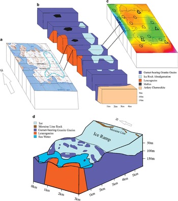
A gravity low within the Garnet-bearing Granite Gneiss unit on Mitchell Peninsula reveals an ice ramp connecting Mitchell Peninsula to the adjacent Law Dome ice cap. This ice ramp has been modelled in detail (Fig. 7). The ice ramp was first modelled assuming that the ice ramp was completely ice, and was assigned a density of 900 kg m-3. This created an ice ramp extending to a depth of approximately 50 m. A more feasible geological model assumes that the ice ramp is made up of approximately half ice and half rock. This assumption is based on the knowledge that the gravity observations were made on isolated rock outcrops (nunataks) and hence there must be a portion of rock within the ice ramp. A model was created assuming that the ice ramp is composed of ice with sporadic rock formations or nunataks. We adopted equal amounts of rock and ice to give an average density of 1800 kg m-3. The eastern extent of the ice ramp could not be defined as there were no in situ rock outcrops apart from the moraine line further up the ice cap slope (Fig. 7d). This model has the ice ramp extending down to a depth of just over 100 m, which is just below sea level, indicating that if this ice ramp were to melt the western half of Mitchell Peninsula would be an island or series of islands separated from the mainland by a marine channel. This has occurred at other places in Antarctica including both Biscoe Point (SCAR 2005) and Stonington Island (Splettstoesser Reference Splettstoesser1992) along the Antarctic Peninsula, where an ice ramp that was once joining the island to an ice cap has melted to leave the island separated from the ice cap by a narrow marine channel. Both of these ice ramps were of similar scale to the Mitchell Peninsula ice ramp proposed in this study.
Block model of the Mitchell Peninsula ice ramp. a. A topography map of Mitchell Peninsula with the lateral surface extents of the modelled ice ramp (turquoise dotted lines). The east–west oriented black lines represent the numerous 1 km thick transects that have been modelled across Mitchell Peninsula. b. A 3D block model that has been sliced along the modelled transects across Mitchell Peninsula. The ice ramp has been modelled to a depth of approximately 115 m. c. Bouguer anomaly image of Mitchell Peninsula. The low anomaly is created by the ice ramp which is less dense than its surrounding crustal rocks. Legend is the same as Fig. 4b. d. A 3D block model of the Mitchell Peninsula ice ramp with each of the sections from Fig. 7b aligned together, and with topography added to provide perspective.

Summary and implications
The reduction and analysis procedures of this study made extensive use of least-squares, especially error propagation, methodology. The results demonstrate that logistically compromised and hence relatively poor Antarctic gravity data can be processed to provide important ‘first cut’ interpretations. In this case, the study area, the Windmill Islands of Wilkes Land, East Antarctica, is the only significant ice-free accessible rock for 400 km in any direction and thus of importance in the field of Antarctic geoscience.
The study has shown that the major rock units in the area, the Ardery Charnockite and the granitic gneiss units, extend to depths of up to 7–13 km and possibly beyond (Figs. 4 & 6). These units are also of considerable lateral extent and typically have steep contacts. The Ford Granite has a steep western contact and extends to a depth of 6–12 km. The Ford Granite pluton either extends to the east at depth, or possibly a blind granitic pluton occurs to the east of the pluton beneath the western portion of Herring Island. The Early Granite Gneiss rock unit which comprises much of Clark Peninsula extends to the north beneath the Swain Group of islands, as suggested by a distinct gravity low. The other major negative anomaly in the area, situated in the vicinity of the islands off the coast of Mitchell Peninsula, is a result of the low density leucogneiss comprising those islands.
The implications for study of the gravity of the nearby Law Dome ice cap, which is generally at an elevation in excess of 1000 m, over a relatively flat, near-zero elevation bedrock/ice interface are that a uniform basement with a density of 2670 kg m-3 would be appropriate for that area. Thus, significant changes in surface gravity are to be initially ascribed to changes in ice thickness.
An ice ramp on the eastern half of Mitchell Peninsula extending to a depth of approximately 100 m has been detected (Fig. 7). This discovery close to Casey Station would allow a study monitoring melting of the ice ramp to be easily undertaken. The ice ramp on Mitchell Peninsula possesses the potential for detailed study of the impact of melting along this part of the East Antarctic coastline by means of precise differential GPS (DGPS) and gravity measurements. In this case, the DGPS data would provide information on the behaviour of the surface at the 2–3 mm level relative to the well-known International GNSS (Global Navigation Satellite Systems) Service (IGS) site at Casey Station, while changes in the observed Bouguer anomaly have the potential to ascribe which part of the ice ramp, the surface with a firn density of 600 kg m-3 or the ice ramp basement with an ice density of 900 kgm-3, is undergoing the greatest melting. Our modelling suggests that this is feasible with today’s automated relative gravity meters which have a least count reading of 0.001 mgal, resulting in an expected signal to noise ratio of four.
Acknowledgements
Firstly, we would like to thank the PhD reviewers whose careful and constructive reviews have greatly improved our manuscript. We would also like to thank the two anonymous reviewers of this paper for their helpful comments. This project drew upon a wide range of resources. We are grateful to all personnel at Casey Station for the 2004–05 summer season, especially Field Training Officer Martin Benevente and the inflatable rescue boat crews. Thanks to Suzanne Haydon and Lindsay Thomas who made available data collected during 1993–94 under ASAC Grant 724. Thanks to Geoscience Australia who made available a Lacoste and Romberg gravity meter (G101) as well as providing excellent library and general technical support. Primary funding and infrastructure was provided by the Australian Antarctic Division under ASAC Grant 2580. Bailey was supported by a Macquarie University RAACE scholarship and a Macquarie University Post-graduate Research Fund (PGRF) grant. Morgan was supported by the University of Canberra Research Fund. This is contribution 1028 from the Australian Research Council National Key Centre for Geochemical Evolution and Metallogeny of Continents (http://www.gemoc.mq.edu.au).
Author contribution
P.J. Morgan conceived the study and co-ordinated the fieldwork. B.T. Bailey and P.J. Morgan undertook the fieldwork. P.J. Morgan processed the site GPS data. B.T. Bailey undertook the primary processing, analysis and modelling of the data. P.J. Morgan and M.A. Lackie undertook secondary modelling and analysis of the data. B.T. Bailey prepared the draft manuscript and all authors contributed to refining the manuscript, with the text finalized by M.A. Lackie.