1. Introduction
Catastrophe (CAT) bonds are insurance-linked securities that transfer extreme, low-frequency risks from insurers to capital markets. They provide insurers with contingent capital for disaster losses while offering investors uncorrelated returns. However, CAT bond pricing remains analytically challenging because payoffs depend on non-Gaussian, discontinuous loss processes and heterogeneous contractual structures. These features produce heavy-tailed distributions, limited liquidity, and nonlinear relationships between expected loss and observed spreads – dynamics that traditional actuarial or no-arbitrage models struggle to explain.Footnote 1
Distortion operator theory provides a flexible actuarial framework that embeds investors’ tail-risk aversion by transforming objective loss probabilities into risk-adjusted measures. The seminal (Wang,Reference Wang2000) transform established this foundation, and subsequent extensions by Denuit et al. (Reference Denuit, Devolder and Goderniaux2007), Chen and Cox (Reference Chen and Cox2009), and Godin et al. (Reference Godin, Lai and Trottier2019) demonstrated its applicability to a broad class of contingent claims. In the CAT bond market, Galeotti et al. (Reference Galeotti, Gürtler and Winkelvos2013) showed that distortion-adjusted and linear specifications outperform traditional pricing rules, highlighting the value of incorporating tail adjustment. Later studies such as Gomez and Carcamo (Reference Gomez and Carcamo2014) and Braun (Reference Braun2016) extended into multifactor settings, combining expected loss with bond characteristics and macro-financial variables. Godin et al. (Reference Godin, Lai and Trottier2019) introduced the JD distortion operator to capture asymmetric and discontinuous tail behavior. More recent work by Herrmann and Hibbeln (Reference Herrmann and Hibbeln2023) emphasized liquidity frictions and repricing dynamics in secondary markets, underscoring the need for models that are both actuarially coherent and empirically adaptive.
Despite these advances, two important gaps remain. First, existing models rely almost exclusively on a bond’s own expected loss – either raw or distortion-adjusted – and have not incorporated distortion-based quantities as explicit factors within multifactor linear pricing models. As a result, prior studies have not examined how distortion-adjusted risk interacts with traditional financial and actuarial determinants. Second, the literature has largely overlooked contemporaneous information from market. As shown in Zhao and Yu (Reference Zhao and Yu2020), CAT bond market-based measures predict subsequent catastrophe losses, indicating that market prices aggregate forward-looking information about catastrophe risk. If market-wide signals forecast CAT risk, they should also help explain CAT bond spreads beyond a bond’s own expected loss. Issuance spreads of bonds with similar underlying peril, covered geographic region, and timing embed valuable signals about prevailing catastrophe risk premia, investor sentiment, reinsurance capacity, and market liquidity. These cross-bond signals have not been incorporated into distortion-operator pricing frameworks.
To address these challenges, we introduce a novel peer-adjusted distortion factor, built upon both the Wang transform (Wang, Reference Wang2000) and the JD distortion operator (Godin et al, Reference Godin, Lai and Trottier2019). This factor calibrates distortion parameters using the market-weighted issuance spread of a peer portfolio (excluding the target bond) – defined by matching bond’s underlying peril, covered geographic region, and a one-year issuance window – together with the target bond’s expected loss. By calibrating to a peer benchmark instead, we obtain a market-implied distortion kernel that reflects the collective valuation of comparable risks. The resulting peer-adjusted factor therefore embeds not only the actuarial information in expected loss but also contemporaneous pricing sentiment, reinsurance capacity constraints, and market liquidity conditions. Empirically, this factor is highly significant in both single- and multifactor settings, improving explanatory and predictive performance beyond traditional covariates. Moreover, the JD-based version of this factor systematically outperforms the Wang-based version in both in-sample and out-of-sample tests, providing a more accurate and economically consistent representation of catastrophe risk premia. These results are consistent with Galeotti et al. (Reference Galeotti, Gürtler and Winkelvos2013), who demonstrated the superior explanatory power of distortion-based frameworks and linear models; however, motivated by Zhao and Yu (Reference Zhao and Yu2020), our approach extends their insights by calibrating distortions through contemporaneous market information. It also advances the linear and multifactor frameworks of Galeotti et al. (Reference Galeotti, Gürtler and Winkelvos2013) and Braun (Reference Braun2016) by embedding the peer-adjusted distortion factor within a multifactor structure that integrates distortion-adjusted expected loss with bond-specific and macro-financial determinants.
From a methodological perspective, parallel advances in machine learning have transformed actuarial risk modeling. Wüthrich (Reference Wüthrich2017), Perla et al. (Reference Perla, Richman, Scognamiglio and Wüthrich2021), Richman and Wüthrich (Reference Richman and Wüthrich2021), and Zhu and Wüthrich (Reference Zhu and Wüthrich2021) showed that neural networks can approximate complex risk-transfer mechanisms while retaining interpretability across P&C insurance, mortality, and related domains. In particular, Chen et al. (Reference Chen, Lu, Zhang and Zhu2024) applied deep learning to weather and index insurance and achieves superior calibration of nonlinear loss-premium relationships. Wei and Jiang (Reference Wei and Jiang2025) further demonstrates that the neural net estimator (NNE) can consistently recover structural parameters in nonlinear dynamic systems, thereby bridging econometric inference with data-driven learning.
Building on these insights, our study employs recurrent neural network (RNN) not merely as predictive tools but as structural estimators of distortion operators. Compared with the nonparametric estimation approach used in Godin et al. (Reference Godin, Lai and Trottier2019), we take a further step forward. Unlike maximum likelihood (MLE), generalized method of moments (GMM), or kernel regression estimators, the RNN approach jointly captures temporal dependence, nonlinear parameter interactions, and tail dynamics intrinsic to catastrophe risk. Relative to other machine learning methods – such as ensemble regressors, gradient boosting, or kernel-based models – the RNN framework uniquely models sequential dependence and evolving parameter dynamics while preserving structural interpretability. This design yields smoother convergence, greater robustness to sample heterogeneity, and improved out-of-sample accuracy. By directly estimating distortion parameters from market data, the RNN provides a flexible yet economically interpretable calibration mechanism, advancing the methodological frontier of distortion-based CAT bond pricing.
In summary, this study contributes to the literature in three main ways. First, it provides theoretical and empirical evidence that the JD distortion operator offers a superior representation of catastrophe risk premia relative to the Wang transform and the raw expected loss of the CAT bond. Second, it introduces an RNN-based estimation method that enhances the accuracy, efficiency, and interpretability of distortion parameter inference compared with MLE, GMM, or ensemble approaches. Third, it identifies and validates a new peer-adjusted distortion factor that robustly explains pricing variation across issuance and trading markets, confirming that multifactor models integrating both actuarial and financial determinants yield the most consistent and predictive performance. By unifying distortion operator theory with neural estimation in a multifactor framework, this paper advances both the methodological and empirical foundations of CAT bond pricing in actuarial science.
The remainder of this paper is organized as follows. Section 2 develops the CAT bond pricing models based on the Wang and JD distortion operators, introduces the peer-adjusted distortion factor, and presents both single- and multifactor specifications. Section 3 describes the data and summary statistics. Section 4 reports the empirical results for the primary and secondary markets. Section 5 concludes.
2. Model
2.1. Distortion operator for CAT bond pricing spread
CAT bonds are financial instruments whose returns depend on the occurrence and severity of natural disasters. Because these events are rare but can generate large losses, investors demand compensation for the associated tail risk. Therefore, a proper pricing model must account for the nonlinearity of disaster risk and for the market’s risk preferences.
The distortion operator framework provides a flexible and theoretically consistent way to incorporate these effects. Instead of taking expectations under the physical probability measure, it reweights tail probabilities through a monotone, concave distortion function
 $ g\,:\,[0,1]\rightarrow[0,1] $
. This adjustment converts the physical loss distribution into a risk-adjusted one, thereby embedding investors’ risk aversion and market sentiment directly into the pricing kernel. The resulting premium can be expressed as a Choquet-type integral of the survival function. Following Galeotti et al. (Reference Galeotti, Gürtler and Winkelvos2013),
 \begin{equation}S = \frac{1}{A} \int_{b}^{b+A} g\!\left(\bar{F}_{X,P}(x)\right)\,dx,\end{equation}
where
 $ \bar{F}_{X,P}(x) = P(X\gt x) $
is the survival probability of loss X under the physical measure P, A is the layer width, and S represents the spread over the risk-free rate. If no triggering event occurs between b and
 $b{+}A$
, the investor receives the coupon reflecting S and the principal at maturity.Footnote
2
Two practical approximations of Equation (2.1) are commonly used. (1) With the probabilities of first and last loss,
 $\text{PFL}=\bar{F}_{X,P}(b)$
and
 $\text{PLL}=\bar{F}_{X,P}(b{+}A)$
, one can apply a trapezoidal rule:
 \begin{equation}S \approx \frac{g(\text{PFL}) + g(\text{PLL})}{2}.\end{equation}
(2) When detailed information on layer edges is unavailable, a rectangular approximation based on the expected loss (EL) may be used:
 \begin{equation}S \approx g(\text{EL}),\qquad\text{EL} \equiv \frac{1}{A}\int_{b}^{b+A}\bar{F}_{X,P}(x)\,dx.\end{equation}
However, as emphasized by Godin et al. (Reference Godin, Lai and Trottier2019), such simplifications can introduce bias. Equation (2.2) would be exact only if
 $g\!\circ\!\bar{F}_{X,P}$
were linear over
 $[b,b{+}A]$
, and Equation (2.3) would be exact only if g were linear over
 $[\bar{F}_{X,P}(b),\bar{F}_{X,P}(b{+}A)]$
. In reality,
 $g\!\circ\!\bar{F}_{X,P}$
is typically convex on that interval – since
 $\bar{F}_{X,P}$
is decreasing and bounded below – so the trapezoidal rule tends to overestimate the true spread. The magnitude and direction of these biases are difficult to assess ex ante and can interact with the calibration of distortion parameters. For this reason, it is essential to choose an appropriate distortion function g and to estimate its parameters carefully.
Remark 2.1. The intuition behind using
 $g(\cdot)$
is that it systematically inflates (or deflates) tail probabilities to reflect investors’ aversion to catastrophe risk. If
 $g(u)\gt u$
for small u, the right tail of the loss distribution receives a higher effective probability under the pricing measure, producing a higher premium S. Conversely, a concave g downweights high-probability, low-loss outcomes. This mechanism captures the observed convexity in the empirical relationship between expected loss and market spread that cannot be replicated by linear pricing rules. Hence, the distortion operator framework not only generalizes actuarial premium principles but also reconciles them with no-arbitrage pricing under risk-adjusted measures.
In this paper, we focus on two families of distortion functions: Wang transform (Wang Reference Wang2000) and JD distortion operator (Godin et al. Reference Godin, Lai and Trottier2019). The Wang transform offers a simple, smooth adjustment to tail risk, while the JD distortion introduces additional flexibility to capture discontinuous jumps and heavy-tailed catastrophe losses observed in CAT bond markets.
2.1.1. Distortion operator pricing model based on Wang transform
The Wang transform (Wang Reference Wang2000) modifies probability distributions through a monotonic distortion function. It is widely used in risk management and insurance pricing to address distributional asymmetry and tail risks (Wang Reference Wang2004; Galeotti et al. Reference Galeotti, Gürtler and Winkelvos2013). In CAT bond pricing, it transforms the original distribution into a risk-neutral one, aligning pricing with market preferences.
This method is particularly useful in modeling rare but severe losses. The mathematical foundation relies on risk-neutral valuation, with the distortion function g defined as:
 \begin{equation}g_\theta(x) = \Phi\left(\Phi^{-1}(x) + \theta\right),\end{equation}
where
 $ \Phi $
denotes the standard normal cumulative distribution function (CDF) and
 $ \theta $
is a parameter that reflects risk aversion. By estimating
 $ \theta $
, the distorted distribution is determined and used for pricing.
2.1.2. Distortion operator pricing model based on jump-diffusion processes
Catastrophe risk is characterized by low frequency but potentially extreme severity. The resulting loss distributions are heavy-tailed and may exhibit abrupt spikes, which pose challenges for pricing approaches that rely on smooth or light-tailed probability structures. While the Wang transform provides a parsimonious way to inflate tail probabilities, it is essentially a static distortion of a normal benchmark and may be too restrictive to capture the discontinuous and time-varying nature of disaster losses. In particular, when catastrophe losses feature jump-like realizations, distortion operators built on purely normal distributions can understate tail behavior and thereby impair risk pricing. Motivated by these stylized features, the CAT bond literature has widely adopted JD and compound Poisson structures to model catastrophe risk and related pricing dynamics (e.g., Lee and Yu Reference Lee and Yu2002; Vaugirard Reference Vaugirard2003; Egami and Young Reference Egami and Young2008; Nowak and Romaniuk Reference Nowak and Romaniuk2013, Parcollet et al. Reference Lai, Parcollet and Lamond2014, and among others).
Building on this line of work, Godin et al. (Reference Godin, Lai and Trottier2019) introduced a distortion operator based on JD processes, which enables dynamic adjustment of loss distributions and provides the first CAT bond evidence that JD structures are empirically appropriate and that investors’ aversion to natural disaster risk is reflected in observed prices. In this setting, JD models capture the possibility of sudden, infrequent, but severe loss shocks – such as those triggered by major catastrophes – thereby rationalizing higher required premia. Accordingly, Godin et al. (Reference Godin, Lai and Trottier2019) proposed a tractable JD distortion operator expressed as a mixture of normal and exponential components, offering a flexible yet interpretable representation of catastrophe-loss tails:
 \begin{equation}g_{\varphi ,\lambda ,\eta, \nu }(u) \equiv \gamma_{\lambda \nu ,\frac{\eta }{\nu }}\left(\gamma_{\lambda ,\eta }^{-1}(u) + \varphi \right),\end{equation}
where u denotes the loss probability,
 $ \lambda \gt 0 $
is the frequency of disaster events,
 $ \eta \gt 0 $
scales the losses,
 $ \nu \geq 1 $
influences tail heaviness, and
 $ \varphi \in \mathbb{R} $
reflects investor risk aversion. The function
 $ \gamma_{\lambda, \eta}^{-1} $
is the inverse of:
 \begin{equation}\gamma_{\lambda ,\eta }(x) \equiv \Pr\left(Z - \sum_{i=1}^{P} Y_i \le x\right), \quad x \in \mathbb{R},\end{equation}
where
 $ Z \sim \mathcal{N}(0,1) $
,
 $ P \sim \text{Poisson}(\lambda) $
, and
 $ Y_i \sim \text{Exp}(\eta) $
are independent.
Remark 2.2. The JD distortion operator provides a theoretically grounded and empirically validated extension of traditional pricing frameworks. Unlike the Wang transform, which applies a smooth and static shift to normal tail probabilities, the JD operator explicitly incorporates discontinuous jumps and heavy tails through a compound Poisson structure. This enables it to capture the low-frequency but high-severity nature of catastrophe losses that dominate the CAT bond market. As shown in Godin et al. (Reference Godin, Lai and Trottier2019), ignoring jump risk aversion leads to systematic pricing biases, particularly at high expected losses.
In this framework, u denotes the loss probability representing the cumulative distribution of market-perceived catastrophe losses. The parameters carry clear economic meaning:
 $\lambda$
denotes the frequency of disaster events, measuring how often catastrophic jumps occur;
 $\eta$
controls the magnitude of these losses, representing market expectations about potential loss severity;
 $\nu$
influences the heaviness of the loss-tail distribution, capturing volatility in extreme events; and
 $\varphi$
is the investor risk-aversion adjustment, describing the market’s subjective repricing of risk after a catastrophic shock. Together, these parameters allow the distortion to adjust flexibly to different peril types, market conditions, and phases of the insurance cycle.
Compared with standard no-arbitrage pricing frameworks, the JD approach more accurately reproduces the jump-like behavior and convex spread-loss relationship observed in CAT bond markets. It retains interpretability –
 $\lambda$
and
 $\eta$
describe the statistical structure of disaster shocks, while
 $\varphi$
embeds behavioral premia – and remains consistent with economic intuition. Although parameter estimation can be computationally demanding, the JD distortion’s ability to reconcile tail risk, discontinuities, and market sentiment makes it a natural and theoretically justified foundation for catastrophe bond pricing.
2.2. Estimating the distortion function Using a RNN
A central challenge in catastrophe bond pricing is the estimation of nonlinear distortion mappings that link expected loss (EL) to required spread (S). In our framework, this mapping
 $g(\cdot)$
is governed either by the Wang (Reference Wang2000) transform, which involves a single risk-aversion parameter or by the four-parameter JD distortion operator in Equation (2.5). The latter requires recovering a parameter vector
 $\vartheta=(\phi,\lambda,\eta,\nu)$
that jointly governs market risk aversion, jump intensity, loss severity, and tail heaviness. Classical approaches such as MLE and GMM estimate these parameters by solving high-dimensional nonlinear optimization problems that match model-implied to observed spreads. However, these methods are computationally expensive, sensitive to initial conditions, and often unstable when parameters interact in complex nonlinear ways within
 $g({\cdot})$
.
To address these issues, we adopt a RNN within the NNE framework proposed by Wei and Jiang (Reference Wei and Jiang2025). Their approach demonstrates that neural networks can be used not as black-box predictors but as structural parameter estimators: the network learns to invert the underlying economic model by recognizing the mapping between observables and latent structural parameters. In particular, the NNE framework interprets parameter estimation as a supervised learning problem trained on simulated data, thereby bypassing the need for explicit likelihood functions or moment conditions. This design yields estimators that are both statistically consistent and computationally scalable, especially for models – like the JD distortion operator – that embed nonlinear, simulation-based pricing components.
Following this framework, we simulate many synthetic sequences
 $\{(\mathrm{EL}_i,S_i)\}_{i=1}^n$
under random draws of
 $\vartheta$
, train the RNN to map each sequence back to its generating parameters, and then apply the trained network once to real data to obtain empirical estimates
 $\widehat{\vartheta}$
.Footnote
3
All pricing remains grounded in the structural relation
 $S=g(\mathrm{EL};\,\widehat{\vartheta})$
, ensuring interpretability and consistency with the distortion-operator framework.
2.2.1. Simulation and estimation procedure
We treat the calibration of the JD distortion model
 $S = g(\mathrm{EL};\, \vartheta)$
as a supervised learning task. Synthetic training samples
 $\{(\mathrm{EL}_i, S_i)\}_{i=1}^{n}$
are generated by randomly drawing parameter vectorsFootnote
4
and computing the corresponding distorted spreads using Monte Carlo approximations of
 $g(\mathrm{EL};\,\vartheta)$
.Footnote
5
The same procedure applies to the Wang transform, where the parameter space is one-dimensional (
 $\theta$
).
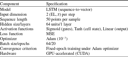
2.2.2. RNN architecture and hyperparameters
We implement a single-layer LSTM sequence-to-vector network with 64 hidden units to estimate the four parameters
 $(\phi, \lambda, \eta, \nu)$
from sequences of 50 normalized
 $(\mathrm{EL}, S)$
pairs. Input normalization serves as an implicit regularization mechanism. The model is trained on GPU using the Adam optimizer (
 $lr = 10^{-3}$
) with MSE loss, batch size 64, for a fixed 20 epochs. Inspection of the loss trajectories confirms stable convergence within these 20 epochs. Early stopping and dropout are omitted, as they do not improve performance and reduce interpretability. The LSTM uses sigmoid activations for the gating functions and tanh for the cell state, while the output layer is linear to produce continuous parameter estimates used in
 $S = g(\mathrm{EL};\, \widehat{\vartheta})$
. Key settings are summarized in Table 1.
RNN configuration for parameter estimation.

2.2.3. Benchmarking framework
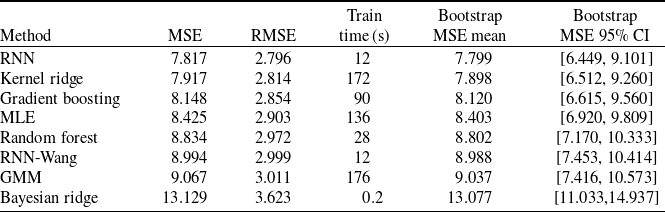
We benchmark the RNN estimator against classical and modern alternatives: MLE, GMM, Kernel Ridge, Gradient Boosting, Random Forest, Bayesian Ridge, and a Wang-RNN baseline. As shown in Table 2, three robust patterns emerge from the benchmark comparison: (1) Fit accuracy. The RNN achieves the lowest MSE and RMSE, indicating the best in-sample fit among all estimators. Kernel Ridge regression attains nearly comparable precision but requires an order-of-magnitude longer training time. MLE and GMM deliver higher residual variance due to their nonlinear optimization burden. (2) Statistical stability. Bootstrap dispersion is narrowest for the RNN, confirming that its fit is not driven by outliers. In contrast, MLE and GMM show wide bootstrap intervals, consistent with local minima sensitivity. (3) Training efficiency. Although deep learning models typically involve longer training phases, our implementation completes in about 12 s – an order of magnitude faster than Kernel Ridge, MLE and GMM, and notably more efficient than Gradient Boosting or Random Forest. After training, the RNN produces parameters and fitted spreads for the full dataset in a single forward pass, whereas likelihood-based estimators require repeated Monte Carlo evaluations. This efficiency, together with the RNN’s compact architecture and vectorized optimization, makes it far more scalable to large CAT bond samples while maintaining high estimation accuracy and numerical stability. Most importantly, even though it uses deep learning, the RNN directly recovers structural parameters
 $(\hat\phi,\hat\lambda,\hat\eta,\hat\nu)$
with clear economic meaning, preserving the transparency of the distortion-operator framework.
Comparison of estimation methods: accuracy, stability, and training efficiency.

Notes: All methods are trained on identical synthetic datasets and evaluated on real CAT bond data using three metrics: (1) Fit accuracy: MSE and RMSE between observed and model-implied spreads; (2) Statistical stability: bootstrap mean and 95% confidence intervals of MSE across bonds; bootstrap statistics are computed via residual resampling. (3) Training efficiency: total seconds required for calibration. Each bond’s own pair
 $(EL_i, S_i)$
is used to estimate the distortion parameters.
Overall, the RNN provides the most favorable trade-off between accuracy, stability, and efficiency while maintaining interpretability. These results justify its use for parameter calibration in JD distortion models and future extensions of CAT bond pricing frameworks.
2.3. A peer-adjusted pricing factor for unobserved issuance spreads
At issuance, a CAT bond’s own spread
 $spread_i$
is precisely the quantity to be priced, making direct calibration of the distortion mapping
 $g({\cdot})$
to its own pair
 $(EL_i, S_i)$
infeasible. Existing distortion-operator studies therefore rely solely on the bond’s expected loss, effectively ignoring contemporaneous pricing information contained in comparable CAT bonds. To overcome this limitation, we introduce a new, economically grounded peer-adjusted distortion factor that extracts a market-implied distortion kernel from the spreads of similar bonds.
For each bond i with peril-region category k(i) and issuance date t(i), we construct a peer benchmark spread as the amount-weighted average of primary-market issuance spreads from CAT bonds issued within the previous 12 months in the same category:
 \begin{equation} \widetilde S^{\,\mathrm{peer}}_{t,k} = \sum_{j\in\mathcal P(t,k)} \omega_j S_j, \qquad \omega_j = \frac{\mathrm{amount}_j}{\sum_{\ell\in\mathcal P(t,k)} \mathrm{amount}_\ell},\end{equation}
where
 $\mathcal P(t,k)$
is the peer set excluding the target bond itself. This peer-adjusted spread captures equilibrium compensation for comparable catastrophe risks and reflects contemporaneous investor sentiment, reinsurance capacity cycles, and liquidity conditions in the CAT bond market.
We then estimate distortion parameters by fitting
 $g({\cdot})$
to the peer benchmark rather than the unobserved target spread:
 \begin{equation}\widehat{\vartheta} = \arg\min_{\vartheta\in\Theta} \sum_{(t,k)} \Big( \widetilde S^{\,\mathrm{peer}}_{t,k} - g(EL_{t,k};\,\vartheta) \Big)^2,\end{equation}
where
 $\vartheta=\theta$
for the Wang transform and
 $\vartheta=(\phi,\lambda,\eta,\nu)$
for the JD distortion operator. This step yields a market-implied pricing kernel that embeds cross-bond information rather than relying solely on the target bond’s expected loss.
For the target bond i, the distortion-adjusted expected loss is then computed as:
 \begin{equation} \mathrm{gel}_i = g(EL_i;\,\widehat{\vartheta}),\end{equation}
where
 $\mathrm{gel} = \{gel_{jd},\, gel_{wang}\}$
denotes the expected loss adjusted under the JD operator and the Wang transform, respectively. This peer-adjusted distortion factor forms the core explanatory variable in our cross-sectional pricing models.
Remark 2.3. The peer-adjusted distortion factor provides both a conceptual and practical innovation. Conceptually, it integrates actuarial distortion theory with market-based information by transforming latent distortion parameters into an observable proxy that reflects the collective valuation of comparable risks. This allows consistent and non-circular calibration even when the bond’s own spread is unavailable at issuance. Practically, the factor offers underwriters and investors a real-time benchmark for assessing fair issuance spreads, while internally incorporating contemporaneous investor sentiment, reinsurance capacity constraints, and market liquidity into the distortion measure.
2.4. Pricing CAT bonds using the peer-adjusted distortion factor
Building on the peer-adjusted factor introduced in Section 2.3, this section incorporates the new factor into formal pricing models. The objective is to examine how well the peer-adjusted distortion variable, derived from Equation (2.9), explains the variation in CAT bond spreads both alone and in conjunction with other structural and market variables. Following Galeotti et al. (Reference Galeotti, Gürtler and Winkelvos2013) and Braun (Reference Braun2016), we consider two complementary specifications: a parsimonious single-factor model and an extended multifactor model. The former isolates the predictive content of the new pricing factor, while the latter evaluates its incremental explanatory power once standard controls are introduced.
2.4.1. Single-factor model
The single-factor model serves as a direct test of whether the peer-adjusted distortion variable encapsulates sufficient information to explain CAT bond spreads in isolation. Specifically, we estimate the following cross-sectional regression:
 \begin{equation} spread_i = \alpha + \beta \, \mathrm{gel}_i + \varepsilon_i,\end{equation}
where
 $spread_i$
denotes the observed primary-market spread and
 $\mathrm{gel}_i$
represents the distortion-adjusted expected loss obtained from the peer-calibrated model. The coefficient
 $\beta$
measures the sensitivity of spreads to distortion-adjusted risk, while the intercept
 $\alpha$
captures systematic risk premia not explained by expected loss alone. A significant and stable
 $\beta$
indicates that the peer-adjusted distortion factor effectively summarizes market pricing of catastrophe risk and provides a structurally grounded single-factor benchmark.
2.4.2. Multifactor model
While expected loss remains the dominant driver of CAT bond spreads, prior studies such as Galeotti et al. (Reference Galeotti, Gürtler and Winkelvos2013) and Braun (Reference Braun2016) highlight the importance of incorporating additional variables reflecting issuance characteristics, contractual design, and market environment. To ensure comparability with the literature and to capture cross-sectional heterogeneity, we extend the model as:
 \begin{align} spread_i = &\, \alpha + \beta_{1} \, \mathrm{gel}_i + \beta_{2} \, \textit{amount}_i + \beta_{3} \, \textit{maturity}_i + \beta_{4} \, \textit{indemnity}_i \nonumber \\[3pt] & + \beta_{5} \, \textit{bbrating}_i + \beta_{6} \, \textit{highyield}_i + \beta_{7} \, \textit{wind}_i + \beta_{8} \, \textit{earthquake}_i \nonumber \\[3pt] & + \beta_{9} \, \textit{us}_i + \beta_{10} \, \textit{japan}_i + \beta_{11} \, \textit{european}_i \nonumber \\[3pt] &+ \beta_{12} \, \textit{multiperil}_i + \beta_{13} \, \textit{reinsurance}_i \nonumber \\[3pt] & + \beta_{14} \, \textit{sp500}_i + \beta_{15} \, \textit{vix}_i + \beta_{16} \, \textit{ted}_i + \beta_{17} \, (\textit{wind} \times \textit{us})_i \nonumber \\[3pt] & + \beta_{18} \, (\textit{earthquake} \times \textit{us})_i + \beta_{19} \, (\textit{wind} \times \textit{japan})_i \nonumber \\[3pt] & + \beta_{20} \, (\textit{earthquake} \times \textit{japan})_i + \beta_{21} \, (\textit{wind} \times \textit{european})_i \nonumber \\[3pt] & + \beta_{22} \, (\textit{earthquake} \times \textit{european})_i + \varepsilon_i.\end{align}
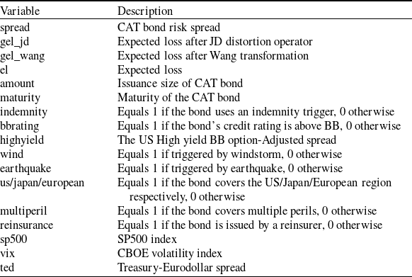
Each additional variable is included to account for structural and market effects documented in the literature. Issuance amount captures liquidity and investor participation; trigger type reflects information transparency and basis risk; maturity and rating proxy duration and credit quality; peril and region dummies control for heterogeneity in disaster exposure; and reinsurance sponsorship proxies counterparty reputation and market cycle conditions. All variables are defined in Table 3, and details are reported in Appendix A.
Variable definitions in the CAT bond pricing model.

To further evaluate the effectiveness of both the new peer-adjusted distortion factor and the underlying distortion operators, we conduct comparative estimations across three alternative measures: the distortion-adjusted expected loss from the JD operator (
 $gel\_jd$
), that from the Wang transform (
 $gel\_wang$
), and the raw expected loss (el) as a baseline. This dual comparison allows us to assess two dimensions of improvement – whether incorporating distortion adjustments enhances explanatory power relative to the traditional linear benchmark, and whether the JD distortion provides additional accuracy beyond the canonical Wang transform. Following the empirical framework of Galeotti et al. (Reference Galeotti, Gürtler and Winkelvos2013) and Braun (Reference Braun2016), we test whether replacing el with structurally distorted or peer-adjusted counterparts improves model fit, parameter stability, and pricing precision. The results, presented in Section 4, show that both the use of distortion-adjusted variables and the peer-adjusted calibration significantly enhance explanatory and predictive performance, confirming the value of our approach as a structural yet empirically tractable pricing framework.
3. Data
The availability of CAT bond trading data is relatively limited, posing challenges in obtaining high-frequency transaction information. This study explores pricing patterns in both the primary and secondary markets for CAT bonds. To address this limitation, we incorporate relevant data from both markets. The primary dataset consists of quarterly CAT bond issuance information from 1999 to 2021, publicly disclosed by LANE FINANCIAL. It includes variables such as Special Purpose Vehicle (SPV), Cedent, S&P Rating, Issuance Amount, Maturity Term, Spread Premium to LIBOR, and Expected Loss. To complement this, additional information on issuance characteristics, trigger types, peril classifications, and covered regions is obtained from ARTEMIS.Footnote 6
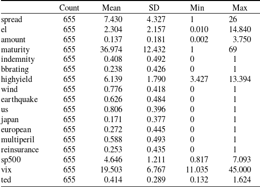
After removing observations with missing values, the final primary market sample contains 655 CAT bond issuances. Table 4 reports descriptive statistics for key variables used in the empirical analysis. The mean spread is approximately 7.43%, with substantial cross-sectional variation (standard deviation 4.33), reflecting heterogeneity in bond risk exposure and structural characteristics. The average expected loss (el) is 2.30%, while the average maturity is around 37 months. Approximately 41% of issuances use indemnity triggers, 24% are rated above BB, and 59% are classified as multi-peril. The inclusion of market-level indicators–such as the US High Yield BB Option-Adjusted Spread (highyield), the S&P 500 index (sp500), the CBOE Volatility Index (vix), and the Treasury-Eurodollar spread (ted) – captures macro-financial conditions influencing bond spreads at issuance.
Descriptive statistics on CAT bond primary market data.

Notes: This table summarizes key variables used in the empirical analysis of primary market CAT bond issuances, sourced from LANE FINANCIAL and ARTEMIS, cover the issuance period 1999–2021. The sample contains 655 observations after excluding records with missing values. spread is measured as the premium to LIBOR at issuance. el denotes expected loss. All variables are defined in Table 3, and details are reported in Appendix A.
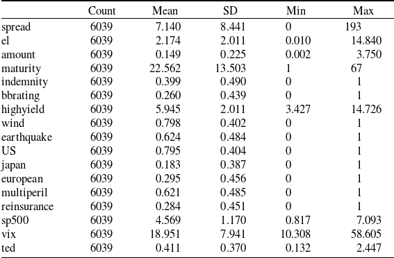
To complement the primary-market evidence, we assemble a panel of secondary-market CAT bond observations to assess pricing consistency over the bond life cycle. Secondary quotes are drawn from the same sources–LANE FINANCIAL and ARTEMIS–for 1999-2021. After removing missing entries, the secondary sample contains 6,039 bond-quarter observations. Table 5 summarizes key variables. Relative to issuance, secondary-market spreads average 7.14 and are more dispersed, consistent with post-issuance trading volatility and liquidity effects. Maturity is shorter by construction (mean 22.6 months). Issuance-time fundamentals (el, amount, peril/region) follow the same definitions as in the primary data, while market-level variables (highyield, sp500, vix, ted) capture time-varying macro-financial conditions that drive repricing.
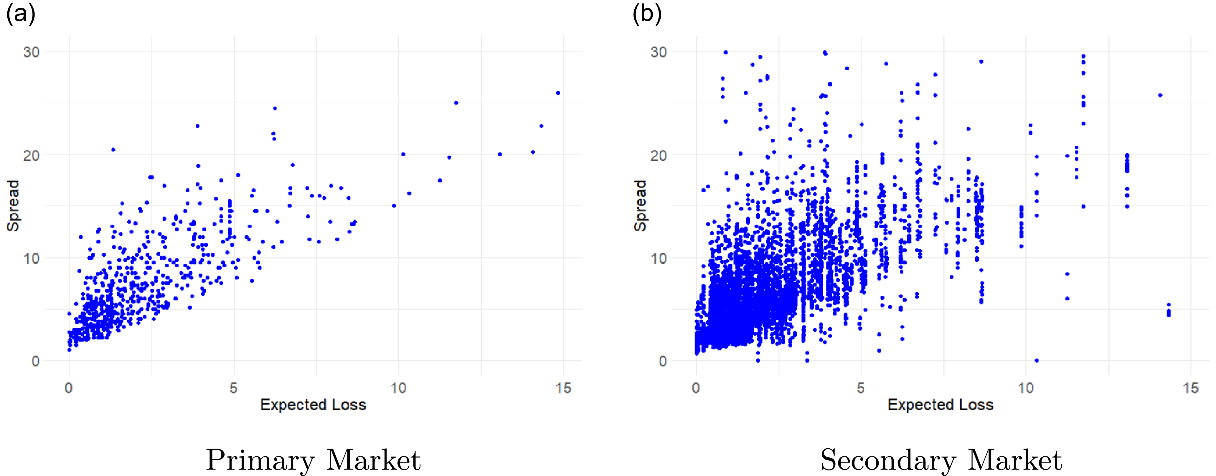
There is a clear positive correlation between CAT bond risk spreads and expected loss. As shown in Figure 1, this relationship holds for both the primary and secondary markets. Notably, most data points are concentrated in the lower range of expected losses, with relatively few observations exceeding 10%. This distribution suggests that linear models may not adequately capture pricing characteristics for bonds with higher expected losses. Furthermore, risk spreads in the secondary market exhibit greater volatility, indicating that additional pricing factors may be necessary to more accurately assess bond values in this market.
Descriptive statistics on CAT bond secondary market data.

Notes: This table reports descriptive statistics for 6039 secondary-market CAT bond observations (1999–2021). Variable definitions are consistent with the primary-market dataset. Secondary-market spreads are more dispersed, while maturities are naturally shorter after issuance. Market-level variables (highyield, sp500, vix, ted) reflect changing macro-financial conditions relevant for repricing.
Risk spreads and expected losses on CAT bonds.
Notes: This figure illustrates the relationship between risk spreads and expected losses for CAT bonds in both the primary and secondary markets. A positive correlation is evident across both markets, indicating that higher expected losses are generally associated with wider risk spreads.

4. Empirical results
4.1. Model fit of the peer-adjusted pricing factor
Building on the estimation framework introduced in Section 2.2, we use the RNN-based NNE to estimate the peer-adjusted distortion parameters defined in Section 2.3. This procedure yields fitted pricing kernels for both the JD and Wang distortion operators, based on the peer-averaged spreads that summarize recent market valuations for comparable catastrophe risks.
Figure 2 displays the model-implied spreads against expected losses. Both specifications reproduce the general concave relationship between CAT bond spreads and expected losses, confirming that the distortion-operator framework successfully captures the nonlinear pricing pattern observed in the market. However, the JD model exhibits a substantially closer alignment with the observed data, particularly in the mid-to-high risk region where nonlinear tail effects dominate. The Wang transform, by contrast, tends to systematically overestimate spreads in the upper tail: when expected loss exceeds roughly 4%, the blue curve consistently lies above both the JD fit and the actual data points. This overpricing arises from the Wang model’s limited flexibility – its single risk-aversion parameter
 $\theta$
produces a uniform shift of tail probabilities that cannot accommodate the jump discontinuities and heterogeneous tail thickness characteristic of catastrophe losses. The JD distortion operator, equipped with parameters controlling jump intensity (
 $\lambda$
), tail heaviness (
 $\nu$
), and exponential scaling (
 $\eta$
), adjusts more dynamically to extreme loss events and thereby avoids systematic bias at high expected loss levels.
Model fit comparison: JD versus Wang distortion.
Notes: This figure compares observed CAT bond spreads (black dots) with model-implied spreads from the JD (red) and Wang (blue) distortion operators. Both models reproduce the nonlinear relationship between spreads and expected loss, but JD fits more closely in the upper tail, where jump-risk and tail-risk effects dominate market pricing.

Residual diagnostics for JD and Wang models.
Notes: The left panel plots residuals (
 $S_{\text{real}} - S_{\text{fitted}}$
) against expected loss. JD residuals (blue) show smaller dispersion and no systematic bias, while Wang residuals (green) drift upward at higher expected losses, confirming overestimation in the upper tail. The right panel displays the residual density distributions, where JD residuals are more symmetric and centered around zero, indicating improved calibration and reduced heteroscedasticity.

Quantitatively, the JD distortion achieves a lower error (MSE = 13.853, RMSE = 3.722) than the Wang distortion (MSE = 15.372, RMSE = 3.921). When using each CAT bond’s own spread and expected loss for estimation, the same pattern holds: the JD model attains a lower MSE of 7.82 compared with 8.99 under the Wang transform (see Table 2). Although the numerical differences appear modest, they are economically significant given the structural heterogeneity of CAT bonds and the pronounced sensitivity of spreads to tail risk. These results underscore that the JD-based peer-adjusted factor offers a more accurate and theoretically coherent representation of market pricing across varying risk regimes.
Residual diagnostics in Figure 3 reinforce these conclusions. In the left panel, the JD residuals (
 $S_{\text{real}} - S_{\text{fitted}}$
) display a centered, pattern-free dispersion across expected losses, implying unbiased estimation and absence of systematic heteroscedasticity. Conversely, the Wang residuals show a clear upward trend for higher expected losses, consistent with overestimation in the upper tail. The right panel presents the residual density comparison: JD residuals are tightly concentrated around zero and approximately symmetric, whereas Wang residuals exhibit right skewness and heavier tails. This pattern confirms that the JD model not only improves mean accuracy but also stabilizes pricing errors, which is critical for robust CAT bond valuation and inference.
Overall, the JD distortion operator demonstrates superior empirical performance in estimating the peer-adjusted pricing factor. It captures nonlinear tail behavior and dynamic jump effects more effectively than the Wang transform, while its parameters (
 $\phi,\lambda,\eta,\nu$
) retain clear economic interpretations linking market risk premia to disaster frequency, magnitude, and investor risk aversion. This fitted JD distortion thus serves as the primary pricing factor in the subsequent single- and multifactor models for CAT bond spreads.
Estimated parameters and fit statistics for distortion models.

Notes: This table reports the estimated parameters and fit performance for the JD and Wang distortion operators, obtained from nonlinear least-squares estimation using peer-adjusted mean spreads. MSE and RMSE denote the mean and root mean squared errors between observed and model-implied spreads. The JD model’s richer parameterization – governing jump intensity (
 $\lambda$
), loss scaling (
 $\eta$
), tail thickness (
 $\nu$
), and investor risk aversion (
 $\phi$
) – allows flexible adjustment to tail behavior, leading to a more accurate and stable fit relative to the Wang transform.
Remark 4.1. Table 6 reports the JD-based distortion estimates
 $\widehat{\vartheta}=(\hat\phi,\hat\lambda,\hat\eta,\hat\nu)=(0.0510, 0.1863,\,4.9357,\,2.7555)$
, and all parameters fall within a plausible interior range for the JD operator. Economically,
 $\hat\phi$
indicates a moderate but clearly positive catastrophe risk premium;
 $\hat\lambda$
implies that the market prices a nontrivial jump component (with an intensity higher than the benchmark magnitude in Godin et al. Reference Godin, Lai and Trottier2019), consistent with investors assigning meaningful weight to rare disaster arrivals in the peer window. The estimates
 $\hat\eta\approx 4.94$
and
 $\hat\nu\approx 2.76$
are close in scale to the JD benchmarks and together imply a heavy right tail for jump losses, that is, severe events receive disproportionate pricing weight. Overall, this parameter configuration produces a distortion kernel that overweights extreme losses relative to moderate ones, which aligns with the observed convex spread-loss relation and explains why the JD specification delivers a tighter fit than the one-parameter Wang transform in both the peer-adjusted calibration and the bond-level benchmarking results.
4.2. Performance of single-factor CAT bond pricing models with peer-adjusted distortion factor in the primary market
4.2.1. In sample test
We begin by evaluating the performance of the single-factor models (Equation 2.10) in explaining CAT bond issuance spreads in the primary market. Columns (1)–(3) of Table 7 correspond to regressions using (1) the raw expected loss (el), (2) the JD-based peer-adjusted factor (
 $gel\_jd$
), and (3) the Wang-based peer-adjusted factor (
 $gel\_wang$
), respectively. All three coefficients are highly significant at the 1% level, confirming that expected loss is a dominant determinant of CAT bond spreads. However, the improvement in model fit from the raw EL specification (
 $R^2=0.592$
) to the distortion-based specifications (
 $R^2=0.610$
for JD and
 $R^2=0.603$
for Wang) indicates that incorporating risk distortions enhances explanatory power. The JD-based factor achieves the best in-sample fit, with an estimated coefficient of
 $0.926$
(s.e.
 $0.051$
). The lower intercept in the JD model (1.394 vs. 3.875 in the EL model and 3.326 in the Wang model) suggests that a significant portion of the excess premium – previously unexplained by EL – is absorbed by the nonlinear tail-risk adjustment captured by the JD distortion.
Parameter estimates of the linear regression model in the primary market.

Notes: This table reports the estimation results of the CAT bond spread models in the primary market. Columns (1)–(3) present the single-factor regressions using the raw expected loss (el),the JD-based peer-adjusted factor (
 $gel\_jd$
), and the Wang-based peer-adjusted factor (
 $gel\_wang$
), respectively. Columns (7)-(9) include all available control variables–bond and market-level factors–representing the full specification of the multifactor model. Columns (4)-(6) employ a parsimonious specification in which the control variables are selected via the LASSO procedure to mitigate multicollinearity while retaining explanatory power. Issuance year and risk group-clustered standard errors are reported in parentheses; significance levels are based on these clustered errors. Asterisks denote significance levels: *
 $p\lt0.1$
, **
 $p\lt0.05$
, ***
 $p\lt0.01$
.
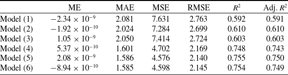
The overall in-sample fit statistics in Table 8 reinforce these conclusions. Model (2), which employs the JD-based peer-adjusted factor, achieves the lowest error (MSE = 7.284, RMSE = 2.699) among the single-factor models, outperforming both the raw EL (MSE = 7.631, RMSE = 2.763) and the Wang-based specification (MSE = 7.414, RMSE = 2.724). Importantly, the peer-adjusted distortion factor also outperforms the single-factor model that relies solely on the JD distortion applied to each bond’s own (EL, S) pair (Table 2, MSE=7.817, without other factors), confirming that incorporating peer market information enhances pricing accuracy.
In-sample performance of the models in the primary market.

Notes: This table compares the in-sample performance of various CAT bond pricing models in the primary market. The metrics include the ME, MAE, MSE, RMSE, and goodness-of-fit measures (
 $R^2$
and adjusted
 $R^2$
).
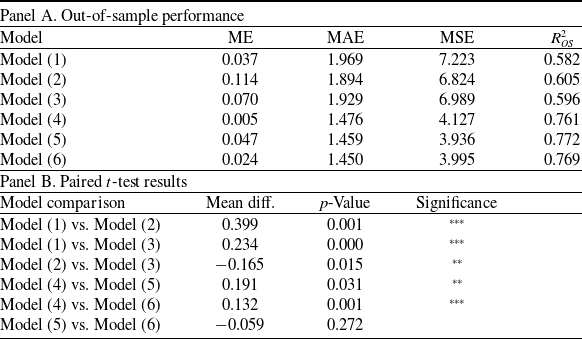
Out-of-sample performance and paired t-tests of the models in the primary market

Notes: This table presents the out-of-sample predictive performance and paired t-test results for various CAT bond pricing models in the primary market. All models are estimated using a random 50–50% data split into training and testing subsets. Panel A reports the ME, MAE, MSE, and the out-of-sample
 $R^2_{OS}$
. Panel B reports the paired t-tests comparing the models’ out-of-sample errors. Asterisks denote significance levels: *
 $p\lt0.1$
, **
 $p\lt0.05$
, ***
 $p\lt0.01$
.
While all models produce mean errors close to zero, Model (2) also delivers a slightly smaller MAE (2.024), indicating better precision in pricing CAT bond spreads. The higher
 $R^2$
and adj-
 $R^2$
values for Model (2) further confirm that its structural flexibility in capturing jump intensity and tail heaviness translates into measurable gains in explanatory power.
4.2.2. Out-of-sample test
Out-of-sample results, presented in Table 9, show that these advantages persist beyond the estimation sample. JD continues to outperform both raw EL and Wang specifications, with lower MSE (6.824 vs. 7.223 and 6.989, respectively) and higher out-of-sample
 $R^2_{OS}$
(0.605 vs. 0.582 and 0.596).Footnote
7
Paired t-tests in Panel B confirm that these differences are statistically significant: the JD-based peer-adjusted single-factor model (Model 2) significantly outperforms the raw EL model (Model 1) at the 1% level (mean MSE difference = 0.399,
 $p=0.001$
) and the Wang-based model (Model 3) at the 5% level (mean MSE difference = 0.165,
 $p=0.015$
). The Wang-based model also outperforms the raw EL at the 1% level. Although the magnitude of improvement may appear modest, the results are economically meaningful given the cross-sectional heterogeneity of CAT bonds and the high sensitivity of spreads to tail-risk misestimation. These findings collectively demonstrate that the peer-adjusted distortion factor, especially the JD-based factor, provides the more accurate and stable single-factor representation of catastrophe risk pricing in the primary market.
4.3. Performance of multifactor CAT bond pricing models with peer-adjusted distortion factor in the primary market
We next evaluate the peer-adjusted distortion factor within an extended cross-sectional setting that augments
 $\mathrm{gel}_i$
with issuance, contractual, peril/region, and market-wide covariates as in Equation (2.11). Table 7 reports three multifactor specifications for each core risk measure: a full model that includes all available controls (Columns (7)–(9)) and a parsimonious model in which controls are selected via adaptive LASSOFootnote
8
to mitigate multicollinearity (Columns (4)–(6)). Then, the multifactor price model (Equation 2.11) changes to:
 \begin{align} spread_i = &\, \alpha + \beta_{1} \, \mathrm{gel}_i + \beta_{2} \, \textit{amount}_i + \beta_{3} \, \textit{maturity}_i + \beta_{4} \, \textit{indemnity}_i \nonumber\\[3pt] & + \beta_{5} \, \textit{bbrating}_i + \beta_{6} \, \textit{highyield}_i + \beta_{7} \, \textit{wind}_i + \beta_{8} \, \textit{earthquake}_i \nonumber\\[3pt] & + \beta_{9} \, \textit{us}_i + \beta_{10} \, \textit{sp500}_i + \beta_{11} \, \textit{vix}_i + \beta_{12} \, (\textit{wind} \times \textit{us})_i \nonumber\\[3pt] & + \beta_{13} \, (\textit{earthquake} \times \textit{us})_i + \beta_{14} \, (\textit{wind} \times \textit{japan})_i + \varepsilon_i.\end{align}
4.3.1. Fit and parsimony
Across multifactor specifications, the JD-based factor remains the top performer. In the LASSO-selected models, Model (5, JD-based) achieves the best in-sample fit among the Columns (4)–(6) of Table 8, exhibiting the lowest MSE (4.576) and RMSE (2.140) and the highest
 $R^2$
(0.755), narrowly outperforming both the raw EL (Model 4) and the Wang-based (Model 6) specifications. Out-of-sample results in Table 9 show a consistent ordering: Model (5) delivers the lowest MSE (3.936) and the highest
 $R^2_{OS}$
(0.772) among the LASSO models. Paired t-tests also confirm that the peer-adjusted distortion factors outperform the raw EL in the multifactor models. The JD-based model (Model 5) and Wang-based model (Model 6) significantly outperform the raw EL model (Model 4) at the 5% level and 1% level, respectively. Although the JD-based and Wang-based models are not statistically different at conventional levels, the JD specification’s stronger economic foundations, combined with its consistently better in-sample and out-of-sample fit, make it the more compelling choice overall. Comparing the full models (7)–(9) yields the same qualitative conclusion: the JD-based specification (Model 8) achieves the best in-sample fit, matching the explanatory power of the full EL and Wang versions while maintaining greater parsimony.
4.3.2. Economic content of controls
Control coefficients line up with the literature. Credit conditions (highyield) load positively and significantly across multifactor specifications, consistent with wider credit spreads raising required CAT bond premia. Market-uncertainty (vix) enters with a small but positive and marginally significant effect, indicating a modest pass-through of broad risk aversion. Interactions such as
 $\textit{US}\times\textit{Wind}$
are economically large and significant, capturing geography-peril premia documented by Braun (Reference Braun2016). After LASSO selection, the resulting model remains stable and interpretable, with reduced collinearity and essentially unchanged
 $R^2$
, indicating that the incremental gains are not driven by overfitting.
Taken together, the multifactor evidence confirms that the JD-based peer-adjusted factor retains superior explanatory power once standard bond-level and market-level controls are introduced. The gains are both statistically and economically meaningful in-sample and out-of-sample. For instance, within the JD specification, the multifactor model attains an in-sample
 $R^2$
of 0.755 versus 0.610 for its single-factor counterpart, while the MSE declines from 7.284 to 4.576 – highlighting the substantial improvement from jointly modeling actuarial and financial determinants. These results reinforce the core premise of the paper: modeling jump intensity and tail heaviness within the distortion operator yields a pricing factor that is structurally grounded and empirically dominant in the primary CAT bond market. Robustness tests with regard to peril-specific subsamples, region-specific subsamples, and different-period subsamples for the multifactor models also confirm this, as detailed in the Appendix B.
4.4. Performance of CAT bond pricing models with peer-adjusted distortion factor in the secondary market
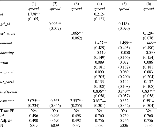
We extend the primary-market evidence to a panel of secondary-market quotes, asking whether the peer-adjusted distortion factor continues to organize pricing once bonds trade post-issuance.Footnote 9 Secondary spreads are observed in an unbalanced panel and are jointly exposed to market-wide shocks; we therefore estimate models with quarter fixed effects (time FE) and, in multifactor settings, include a lagged dependent variable to capture price inertia.
4.4.1. Single-factor models with time fixed effects
We begin by isolating the pricing content of the peer-adjusted distortion factor in a panel setting. Consistent with the primary-market analysis, we estimate a single-factor pricing model in the secondary market. However, unlike the (cross-sectional) issuance data, secondary quotes form an unbalanced panel in which spreads are jointly exposed to common time-varying shocks – such as fluctuations in global risk appetite, funding conditions, and the reinsurance cycle. These features motivate the inclusion of quarterly time fixed effects (time FE) to absorb market-wide shocks that move all bonds in tandem.Footnote 10
Formally, the time-FE single-factor model is specified as:
 \begin{equation}\textit{spread}_{i,t} = \alpha + \beta\,\mathrm{gel}_{i,t} + \tau_t + \varepsilon_{i,t},\end{equation}
where
 $\tau_t$
denotes quarter dummies capturing contemporaneous shocks common to all CAT bonds.
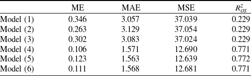
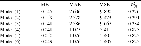
Columns (1)–(3) of Table 10 report the in-sample estimates. Out-of-sample performance is evaluated using both time- and ID-based splits (see Tables 11 and 12). Consistent with the primary-market findings, the JD-based peer-adjusted distortion factor matches or exceeds the explanatory power of alternative specifications across all metrics – yielding lower MSE and MAE and higher
 $R^2_{OS}$
. This result indicates that peer-calibrated tail-risk adjustments remain informative even after accounting for market-wide temporal variations.
In-sample regression results with time fixed effects (secondary market).

Notes: Columns (1)–(3) report time-FE single-factor models using el,
 $gel\_jd$
, and
 $gel\_wang$
, respectively. Columns (4)–(6) report time-FE multifactor models with one-period lagged spread. To mitigate the influence of extreme observations, the secondary-market data are winsorized at the 1st and 99th percentiles. Standard errors are clustered by year and id; asterisks denote *
 $p\lt0.1$
, **
 $p\lt0.05$
, ***
 $p\lt0.01$
.
Out-of-sample performance of models based on time-division.

Notes: Train on data up to 2019; test on 2020+. Models (1)–(3): single-factor; Models (4)–(6): multifactor. The reported ME, MAE, MSE, and
 $R^2_{OS}$
are calculated on the test sets.
4.4.2. Multifactor models with time fixed effects and lagged spread
Building on the preceding single-factor framework, we extend the analysis to a dynamic multifactor specification. In addition to the unbalanced panel structure and common time shocks discussed above, secondary-market spreads also exhibit pronounced price inertia, arising from gradual information diffusion, trading frictions, and liquidity constraints. These features motivate a specification that includes quarterly time fixed effects to absorb contemporaneous market-wide shocks and a lagged dependent variable to capture serial dependence in pricing dynamics. The inclusion of the lag term
 $\textit{lag(spread)}$
parsimoniously accounts for persistence that would otherwise bias coefficient estimates on the structural covariates.
Out-of-sample performance of models based on ID-division.

Notes: Train on a random 80% of bonds; test on the remaining 20%. Models (1)–(3): single-factor; Models (4)–(6): multifactor. The reported ME, MAE, MSE, and
 $R^2_{OS}$
are calculated on the test sets.
To capture cross-sectional heterogeneity and retain comparability with Section 4.3, we augment Equation (4.2) with issuance, contractual, and market covariates, as well as a one-period lag of spreads to capture price inertia:
 \begin{equation}\textit{spread}_{i,t} = \alpha + \beta_1\,\mathrm{gel}_{i,t} + \boldsymbol{\beta}'\mathbf{X}_{i,t} + \rho\,\textit{spread}_{i,t-1} + \tau_t + \varepsilon_{i,t},\end{equation}
where
 $\mathbf{X}_{i,t}$
collects bond characteristics, peril/region dummies and their interactions, and market-level variables (see Equation (2.11)), while
 $\tau_t$
denotes quarter fixed effects capturing contemporaneous common shocks. To mitigate multicollinearity, we employ an adaptive LASSO for control selection as well. Formally, the time-FE multifactor model is specified as:
 \begin{align}\textit{spread}_{i,t} = \alpha & + \beta_{1}\,\mathrm{gel}_{i,t}+ \beta_{2}\,\textit{amount}_{i,t}+ \beta_{3}\,\textit{bbrating}_{i,t}+ \beta_{4}\,\textit{highyield}_{t} \nonumber \\[3pt]& + \beta_{5}\,\textit{wind}_{i}+ \beta_{6}\,(\textit{us}\times\textit{wind})_{i}+ \beta_{7}\,(\textit{us}\times\textit{earthquake})_{i} \nonumber \\[3pt]& + \beta_{8}\,\textit{sp500}_{t}+ \beta_{9}\,\textit{vix}_{t}+ \rho\,\textit{spread}_{i,t-1}+ \tau_{t}+ \varepsilon_{i,t}.\end{align}
Columns (4)–(6) of Table 10 present estimates for the raw/JD/Wang versions, respectively.Footnote
11
The lag is highly significant (
 $\rho\approx 0.84$
) and materially reduces RMSE, while the JD-based specification (Model 5) delivers the best fit among the three, mirroring the primary-market ordering. Robustness test of models without time fixed effects and with/without lagged spread can be found in Appendix C.
4.4.3. Out-of-sample performance and contrast with the primary market
We evaluate six specifications out-of-sample using both a time split (train: data up to 2019; test: 2020+) and an ID split (train: 80% of bonds; test: 20%). In each split, Models (1)–(3) are single-factor time-FE regressions based on el,
 $gel\_jd$
, and
 $gel\_wang$
; Models (4)–(6) are the corresponding multifactor time-FE models. Tables 11 and 12 show that the JD-based peer-adjusted distortion factor (Models 2 and 5) are consistently competitive and typically attain the lowest errors and highest
 $R^2_{OS}$
within each block.
As in Section 4.2, the ordering across pricing factors is stable: JD
 $\gt$
Wang
 $\gt$
EL. The secondary market exhibits larger gains from including dynamics, reflecting persistence that cannot be captured by cross-sectional controls alone; nonetheless, the JD factor retains incremental predictive content once controls and dynamics are in place.
Overall, the JD-based peer-adjusted factor remains the most accurate and stable organizing variable for secondary-market CAT bond pricing, consistent with – and complementary to – the primary-market results.
5. Conclusion
This paper develops an integrated framework for catastrophe bond pricing that unifies distortion operator theory with RNN-based estimation. By combining actuarial tail-risk adjustment with data-driven parameter learning, the approach enhances both theoretical coherence and empirical applicability.
A novel peer-adjusted distortion factor is introduced to address the identification challenge at issuance, embedding contemporaneous investor sentiment, reinsurance capacity, and market liquidity into the distortion measure. This factor remains highly significant across both primary and secondary markets, improving explanatory and predictive performance beyond traditional covariates. Empirical evidence shows that the JD distortion operator consistently outperforms the Wang transform in capturing nonlinear and discontinuous pricing dynamics. The RNN estimator further improves parameter accuracy, robustness, and efficiency while preserving structural interpretability, establishing neural networks as an effective tool for structural estimation in actuarial models. Extending the analysis to a multifactor specification demonstrates that catastrophe bond spreads reflect layered sources of risk. The multifactor models consistently outperform their single-factor counterparts, confirming that combining distortion-adjusted measures with financial and bond-specific determinants yields a more comprehensive and robust pricing framework.
Overall, integrating distortion operators with neural estimation offers a coherent, interpretable, and empirically validated foundation for CAT bond pricing, advancing both actuarial science and financial risk modeling.
Supplementary material
The supplementary material for this article can be found at https://doi.org/10.1017/asb.2026.10089
Acknowledgments
We would like to thank Zhuo Jin, Hong Li, Shaun S. Wang, Feier Yan, Yaodi Yong, Lianzeng Zhang, Hui Zhao, Yang Zhao, and conference participants at the Third International Conference on Actuarial Science, Quantitative Finance and Risk Management. The authors contributed equally to this article. All remaining errors are ours.
Financial support
This research was supported by the MOE (Ministry of Education in China) Liberal Arts and Social Sciences Foundation No. 24YJA790002.
Competing interests
On behalf of all authors, the corresponding author states that there is no conflict of interest.