

I. Introduction
Rietz (Reference Rietz1988) hypothesized that rare and severe macroeconomic disasters could help resolve the equity premium puzzle (Mehra and Prescott (Reference Mehra and Prescott1985)), an idea later revitalized by Barro (Reference Barro2006). Since then, rare disasters have garnered significant attention from both academic researchers and market participants.Footnote 1 Recent research has emphasized the importance of modeling the time variation in disaster risk. Unlike models assuming a constant probability of disasters, frameworks that allow for time-varying disaster probabilities can generate a volatile equity premium and account for several macro-finance puzzles, such as excess volatility and return predictability (Gabaix (Reference Gabaix2012), Gourio (Reference Gourio2012), and Wachter (Reference Wachter2013)). However, empirical estimation of time-varying probabilities of consumption disasters (henceforth, TVPCD) remains highly challenging, which in turn undermines a critical foundation of rare-disaster models.
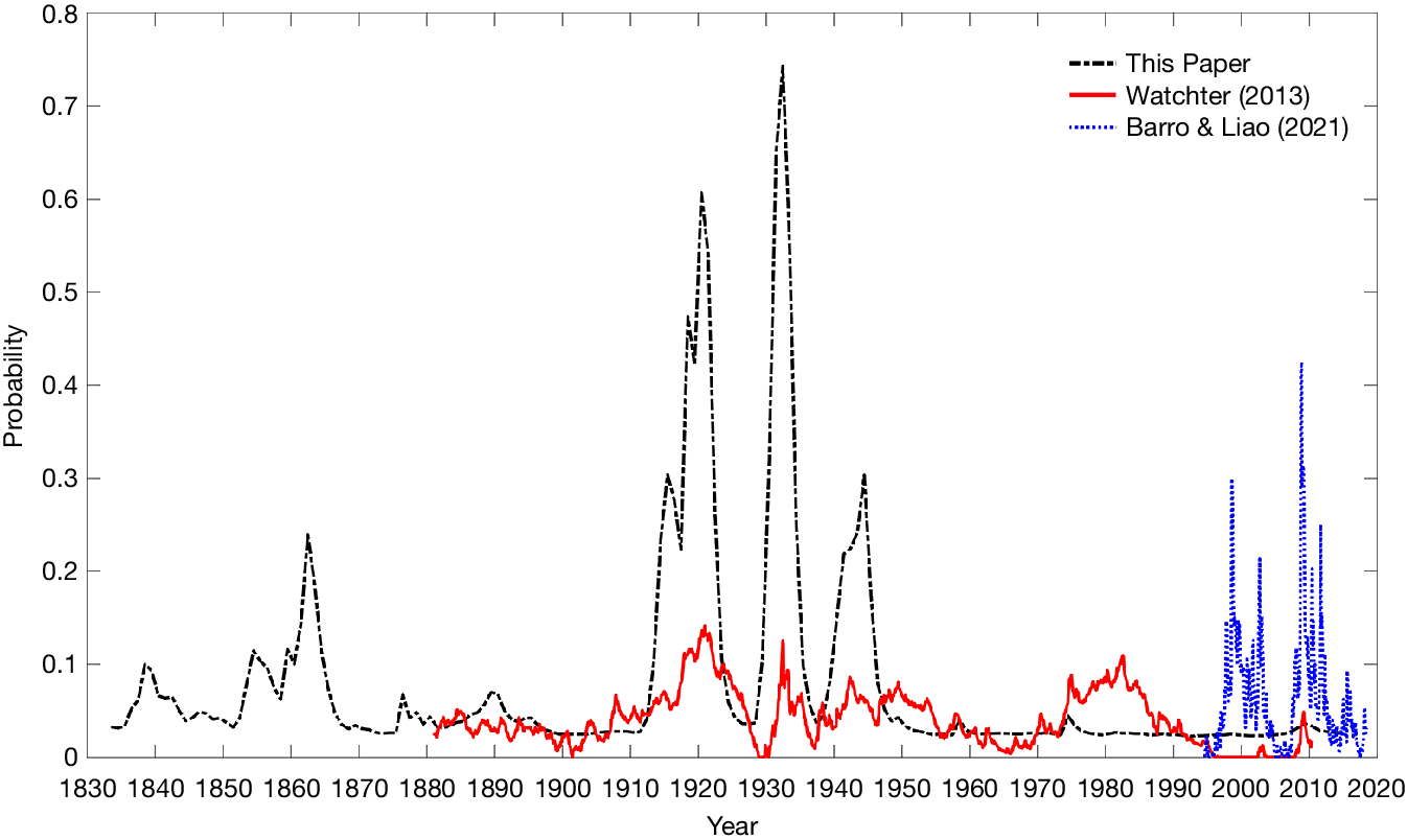
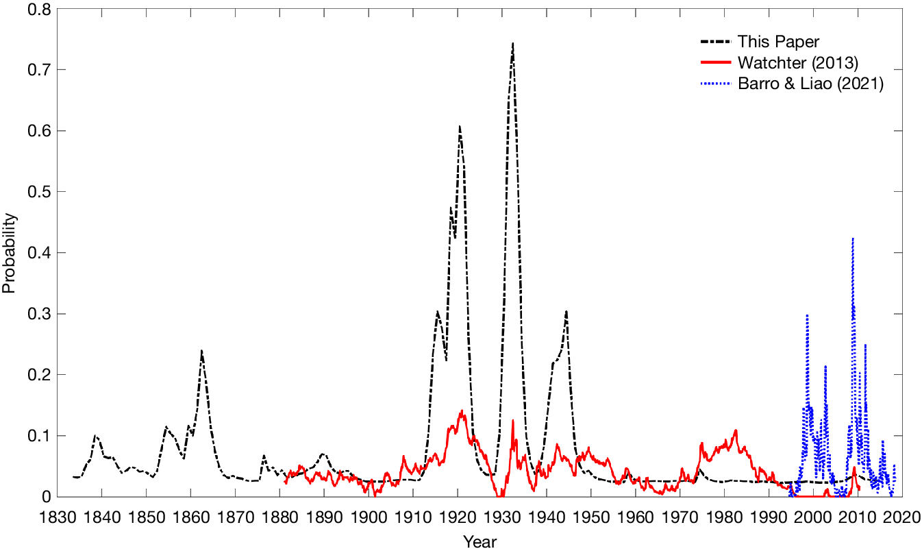
To date, most of the literature has relied on indirect measures of disaster risk inferred from asset prices (Barro and Liao (Reference Barro and Liao2021), Bollerslev and Todorov (Reference Bollerslev and Todorov2011), and Wachter (Reference Wachter2013)). However, these measures often reflect investors’ subjective perceptions rather than the actual probability of disasters and may also incorporate risk factors unrelated to disaster risk. More importantly, inferring disaster probabilities from asset prices introduces a circularity problem, making it difficult to establish an independent, objective estimate of disaster risk. Consequently, disaster risk has been described as “dark matter for economists” (Campbell (Reference Campbell2017), Chen, Dou, and Kogan (Reference Chen, Dou and Kogan2024)). Given these limitations, researchers have sought to construct direct measures of disaster risk using proxy variables that predict consumption disasters (Baron, Xiong, and Ye (Reference Baron, Xiong and Ye2022), Berkman, Jacobsen, and Lee (Reference Berkman, Jacobsen and Lee2011), and Manela and Moreira (Reference Manela and Moreira2017)). In this article, we propose an alternative method that directly estimates the physical (or “real”) probability of time-varying consumption disasters from historical consumption data. As an immediate demonstration, Figure 1 compares our estimated disaster probabilities for the United States with those implied by Wachter (Reference Wachter2013) and Barro and Liao (Reference Barro and Liao2021). Our estimates yield results comparable to those in the existing literature, and for key historical macroeconomic events such as World War I, World War II, and the Great Depression, our model produces disaster probability levels and dynamics that align more closely with common historical narratives.
Figure 1 plots the time-varying consumption disaster probabilities for the United States estimated in this paper (black dashed line) compared with those implied by Wachter (Reference Wachter2013) (red solid line) and Barro and Liao (Reference Barro and Liao2021) (blue dotted line). The estimates from this paper are based on the posterior mean of the disaster probability index derived from long-term national accounts data.
In this article, we propose a new consumption disaster model with time-varying disaster probabilities. In our model, the world and the countries are connected through the international interactions of the world and country-specific disasters and their disaster probabilities. Using long-term national accounts data for 42 economies, we estimate the parameters for the processes of consumption disasters and disaster probabilities. With the estimated disaster model, we back out the coefficient of risk aversion and analyze the asset-pricing implications of the consumption disaster risk.
Our model carefully characterizes both consumption disasters and their probability dynamics. The time-varying probabilities of global and country-specific consumption disasters follow logistic functions of disaster probability indices, which evolve as autoregressive processes with occasional jumps. Specifically, jumps in the global disaster probability index arise from world disasters and unexpected events in the previous period, whereas jumps in country-specific disaster probability indices are driven by unexpected idiosyncratic shocks, current world disasters, and past country-specific disaster dynamics.
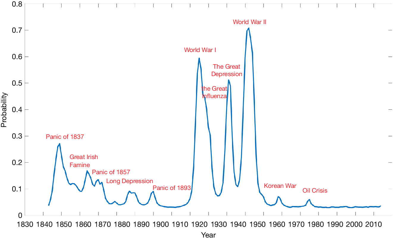
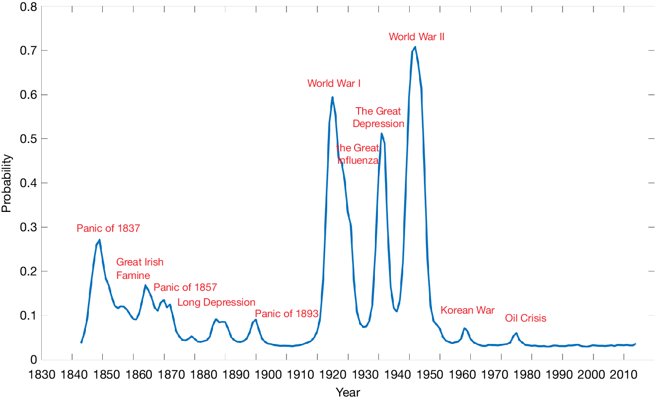
Our first set of findings pertains to the identification of global and country-specific consumption disasters. At the world level, the estimated disaster periods—with the posterior disaster probability of 25% or more—include 1838–1839, 1913–1921, 1930–1933, and 1939–1945, and those with the posterior probability exceeding 50% include 1914–1916, 1931, and 1940–1944. These periods correspond to familiar historical disasters, such as the world wars, the Great Depression, and possibly the Great Influenza Epidemic of 1918–1920 (but not the recent Great Recession of 2007–2009). Figure 2 depicts our estimates of the world disaster probabilities. We also identified many familiar disastrous events for individual countries and small groups of countries, including the First Sino-Japanese War for China in 1895, the Russian Revolution and Civil War during 1917–1922, the 1973 Chilean coup and its aftermath, the Argentinean stagnation and hyperinflation during 1988–1991, and the government-debt crisis and recession in Greece during 2010–2012. The graphs of country-specific disaster probabilities are shown in Section IV.D and in Supplementary Material Section H.
Figure 2 displays the posterior mean of the world disaster probability estimated from the model. Major historical events coinciding with probability peaks are labeled.
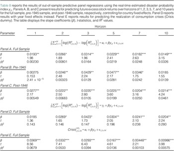
The second set of findings is about the asset-pricing implications of the estimated consumption disaster model. Matching the observed long-term average real rates of return on corporate equity and short-term government bills requires a coefficient of relative risk aversion (CRRA) of 5.2, which is significantly lower than the typical estimates from rare-disaster models. In addition, this model can also quantitatively replicate the predictability of excess stock returns by the dividend yield, as demonstrated in Campbell and Shiller (Reference Campbell and Shiller1988), Cochrane (Reference Cochrane1992), and so forth. One major challenge for general equilibrium models of the stock market is to generate long-run predictability in excess stock returns without producing counterfactual predictability in consumption growth. Our model addresses that challenge, as the estimated dividend yield effectively predicts excess stock returns over extended horizons while exhibiting minimal predictability for consumption growth. This finding aligns with empirical evidence from studies such as Beeler and Campbell (Reference Beeler and Campbell2012), Campbell (Reference Campbell2003), and Lettau and Ludvigson (Reference Lettau and Ludvigson2001). Among other asset-pricing statistics, we also find evidence of the out-of-sample predictability of equity premia from our model’s estimated disaster probability index. That is, a higher disaster probability today predicts a higher average future excess stock return over long horizons. The predictive power of the disaster probability index is notably significant in both time series and cross-sectional contexts.
Unlike prior studies that indirectly estimate disaster probabilities from asset prices, we construct a direct, time-varying measure of macroeconomic disaster probabilities using historical national accounts data, independent of financial data or assumptions about investor preferences. Additionally, our TVPCD model explicitly models the time-series dynamics of global and country-specific disaster probabilities, which are of intrinsic importance in macroeconomics and asset pricing. Substantial efforts have been made in the literature to improve the estimation of disaster risk; our approach offers a novel perspective on measuring disaster risk and provides empirical support for the rare disaster hypothesis through an alternative methodology.
The rest of the article is organized as follows: Section II relates our study to the previous literature on the TVPCD. Section III lays out our formal model. Section IV discusses the data used in this study, describes our method of estimation, and presents empirical results, including a detailed description of six illustrative countries. Section V presents the framework for asset pricing and draws out the implications of the estimated consumption processes for CRRA and various statistics, including the average equity premium and the volatilities of equity returns and premia. Section VI explores the real-time predictability from our estimated disaster probability index. Section VII concludes.
II. Relation to the Literature
Since the seminal work of Rietz (Reference Rietz1988) and Barro (Reference Barro2006), rare-disaster models have been widely recognized for their ability to rationalize asset-pricing puzzles. These models emphasize that even the mere possibility of rare but severe macroeconomic disasters—such as wars, natural disasters, financial crises, and pandemics—can significantly influence asset valuations, investment decisions, and real economic outcomes.
Early rare-disaster models, such as those in Barro (Reference Barro2006), (Reference Barro2009), Barro and Ursúa (Reference Barro and Ursúa2008), and Barro and Jin (Reference Barro and Jin2011), assume a constant probability of disasters. Later models, such as Nakamura, Steinsson, Barro, and Ursúa (Reference Nakamura, Steinsson, Barro and Ursúa2013) and Barro and Jin (Reference Barro and Jin2021), allow disaster probabilities to vary over time and take on several different values, but this variation is directly contingent upon the actual occurrence of disasters. As a result, these models struggle to explain large financial market fluctuations during periods when no consumption disasters are observed. This limitation highlights the need to model disaster probabilities as time-varying and less tightly linked to the actual occurrence of disasters.
A notable step in this direction is Gabaix (Reference Gabaix2012), which discusses time-varying disaster probabilities but does not provide a detailed empirical implementation or parameter calibration. Wachter (Reference Wachter2013) advances the literature by proposing a model with time-varying disaster probabilities, which can generate a volatile equity premium and reconcile several macro-finance anomalies, including excess volatility and return predictability. However, the highest disaster probability estimated in Wachter (Reference Wachter2013)—14% in 1920—appears much lower than what historical records suggest (see Figure 1).
Disaster risk is described as “dark matter” in economic models because it is difficult to directly measure due to its rarity. The existence of this dark matter poses a fundamental challenge to the key assumptions of rare-disaster models. Many studies have attempted to measure disaster risk using various approaches. The existing literature has largely relied on indirect proxies of disaster risk derived from asset prices. For example, several studies have explored measures obtained from option prices (Backus, Chernov, and Martin (Reference Backus, Chernov and Martin2011), Bollerslev and Todorov (Reference Bollerslev and Todorov2011), and Seo and Wachter (Reference Seo and Wachter2019)) or from the cross section of asset returns (Kelly and Jiang (Reference Kelly and Jiang2014)). Siriwardane (Reference Siriwardane2015) constructs a jump risk factor based on short-term option prices for a broad panel of U.S. firms, arguing that this factor proxies for the variation in the risk-neutral probability of macroeconomic disasters. Similarly, Barro and Liao (Reference Barro and Liao2021) propose an option-pricing model incorporating recursive preferences and apply it to far-out-of-the-money put options on the aggregate stock market. Their estimated disaster probabilities fluctuate sharply, spiking during the global financial crisis and peaking at 42% in 2008. While asset prices are highly sensitive to disaster risk, using them to measure disaster probabilities presents a fundamental challenge: The circular nature of extracting disaster probabilities from asset prices raises concerns about whether these estimates truly reflect objective disaster probabilities or are merely self-referential. Moreover, disaster probabilities inferred from financial markets rely on specific assumptions about investor preferences and can be confounded by other risk factors unrelated to disaster risk. As a result, the absence of direct measures of disaster risk has given rise to the argument that financial markets may at times underplay the real threat of disasters (Baron and Xiong (Reference Baron and Xiong2017), Muir (Reference Muir2017)).
A number of studies have attempted to address this challenge by using proxy variables likely to capture variation in tail risk. Baron et al. (Reference Baron, Xiong and Ye2022), for example, propose a measure based on credit expansions and asset bubbles, building on evidence that credit booms often precede banking crises and deep recessions. Berkman et al. (Reference Berkman, Jacobsen and Lee2011) construct a crisis index from a broader set of international political events to reflect perceived disaster risk. Manela and Moreira (Reference Manela and Moreira2017) develop a news-based uncertainty index by linking Wall Street Journal front-page coverage to the CBOE Volatility Index (VIX). More recently, Adrian, Boyarchenko, and Giannone (Reference Adrian, Boyarchenko and Giannone2019) and Marfè and Pénasse (Reference Marfè and Pénasse2024) use quantile regressions to estimate macroeconomic tail risks, with the latter deriving time-varying disaster probabilities by weighting predictors according to their ability to forecast the conditional distribution of consumption growth, using a rich international data set covering macroeconomic, political, and financial variables.
Our study contributes to this literature by proposing a direct, data-driven measure of time-varying disaster probabilities based solely on historical consumption data. Unlike existing approaches that rely on asset prices, preference assumptions, or proxy variables, we estimate the disaster probability process within a unified framework using a long-span international data set and Bayesian Markov chain Monte Carlo (MCMC) methods. Importantly, all model parameters are jointly estimated within this coherent structural framework, in contrast to much of the existing literature that relies on calibrating parameters separately—making our characterization of disaster risk more internally consistent and empirically credible. Our model distinguishes between transitory and permanent consumption shocks and captures global and country-level disaster dynamics. As a result, it not only aligns closely with historical macroeconomic crises but also delivers strong out-of-sample predictability for excess stock returns, offering robust empirical support for the time-varying disaster risk hypothesis.
III. The Model
Our model builds on the framework of Nakamura et al. (Reference Nakamura, Steinsson, Barro and Ursúa2013), a modified version of the Lucas Tree model that allows disasters to unfold over multiple years and be followed by systematic recoveries. This structure provides a more realistic depiction of consumption dynamics and addresses a key limitation of the Rietz–Barro framework—namely, its tendency to overstate risk by assuming instantaneous and complete consumption drops without recovery, as noted by Constantinides (Reference Constantinides2008), Donaldson and Mehra (Reference Donaldson, Mehra and Mehra2008), and Julliard and Ghosh (Reference Julliard and Ghosh2012).
The primary innovation of our model relative to Nakamura et al. (Reference Nakamura, Steinsson, Barro and Ursúa2013) and Barro and Jin (Reference Barro and Jin2021) is the introduction of time-varying disaster probabilities. We also implement several refinements: i) Disaster gaps are assumed to shrink only during normal periods, avoiding the entanglement of multiple effects during disasters, and ii) we allow for serial correlation in the immediate effects of disasters and correlation between immediate and permanent effects, extending beyond the IID assumptions of prior models. The detailed model setup is presented below.
A. Components of Consumption
Similar to previous rare-disaster models, the logarithm of consumption per capita for country
 $ i $
at time
 $ t $
,
 $ {c}_{it} $
, is assumed to be the sum of three unobserved variables:
 $$ {c}_{it}={x}_{it}+{z}_{it}+{\sigma}_{\varepsilon i}{\varepsilon}_{it}, $$
where
 $ {x}_{it} $
is the “potential level” of the logarithm of per capita consumption and
 $ {z}_{it} $
is the “disaster gap,” which describes the deviation of
 $ {c}_{it} $
from its potential level due to current and past consumption disasters. The potential level of consumption and the disaster gap depend on the disaster process, as detailed below. The term
 $ {\sigma}_{\varepsilon i}{\varepsilon}_{it} $
is a temporary shock, where
 $ {\varepsilon}_{it} $
is an IID standard normal variable. The standard deviation,
 $ {\sigma}_{\varepsilon i} $
, of the shock varies by country. We also allow
 $ {\sigma}_{\varepsilon i} $
to take on two values for each country, one up to 1945 and another thereafter. This treatment allows for post-WWII moderation in observed consumption volatility, particularly because of improved measurement in national accounts—see Romer (Reference Romer1986) and Balke and Gordon (Reference Balke and Gordon1989).
B. Time-Varying Disaster Probabilities
We assume that for the whole world and an individual country, there are disaster and normal states. Each state tends to persist over time, but there are varying possibilities for transitioning from one state to the other. The disaster probabilities are determined by the world and country-specific processes.
Let
 $ {I}_{wt} $
be the dummy variable for the presence of a world disaster with
 $ \mathit{\Pr}\left({I}_{wt}=1\right)={p}_{wt} $
. The probability of a world disaster in time
 $ t $
,
 $ {p}_{wt} $
, is assumed to be
 $$ {p}_{wt}=F\left({y}_{wt}\right)=\frac{1}{1+{e}^{-{y}_{wt}}}, $$
where
 $ F\left(\cdot \right) $
is a logistic function and
 $ {y}_{wt} $
is the world disaster probability index at time
 $ t $
. In the evolvement of the world disaster probability, there are jumps that are caused by either unexpected events or disasters in previous periods. Specifically, we assume that the world disaster index
 $ {y}_{wt} $
evolves according to the following equation:
 $$ {y}_{wt}={y}_w^{\ast }+{\rho}_{y_w}\left({y}_{w,t-1}-{y}_w^{\ast}\right)+{K}_{wt}{J}_{wt}^{(1)}+{I}_{w,t-1}{J}_{wt}^{(2)}+{\sigma}_{y_w}{\zeta}_{wt}, $$
where
 $ {\zeta}_{wt} $
is an IID standard normal variable,
 $ {\rho}_{y_w} $
is the first-order autoregressive coefficient, and
 $ {y}_w^{\ast } $
is the mean-reverting value of
 $ {y}_{wt} $
if there are no jumps.
 $ {K}_{wt} $
is a dummy variable with
 $$ \mathit{\Pr}\left({K}_{wt}=1\right)={p}_K, $$
for some
 $ {p}_K>0 $
, and
 $ {J}_{wt}^{(1)} $
and
 $ {J}_{wt}^{(2)} $
stand for jumps whose sizes follow a two-sided power-law distribution with density function
 $$ {f}_{J_w}(s)={\beta}_{J_w}{\left(|s-{m}_w|+1\right)}^{-{\alpha}_{J_w}}, $$
where
 $ {\beta}_{J_w}=\left({\alpha}_{J_w}-1\right)/2 $
, and
 $ {m}_w $
and
 $ {\alpha}_{J_w} $
are all constant parameters characterizing the location and shape of the power-law distribution.Footnote
2 Here,
 $ {J}_{wt}^{(1)} $
describes the jump that is triggered by an unexpected world event in period
 $ t $
, and this trigger is effective only when
 $ {K}_{wt}=1 $
;
 $ {J}_{wt}^{(2)} $
describes the jump that is caused by the world disaster in period
 $ \left(t-1\right) $
. Both of these jump terms are introduced to accommodate the rapid growth of the index during disaster periods. Specifically,
 $ {K}_{wt}{J}_{wt}^{(1)} $
aims to account for unexpected shocks that lead to a sharp rise in the disaster index
 $ {y}_{wt} $
, particularly when the probability of the economy transitioning from a normal state to a disaster state abruptly rises. The dummy variable
 $ {K}_{wt} $
is introduced to indicate the occurrence of such unexpected and usually rare shocks. The second jump term
 $ {I}_{w,t-1}{J}_{wt}^{(2)} $
considers the persistency of the disaster state, where a disaster state in the previous period tends to keep the probability of subsequent disasters at a high level.
For each country, similar to the process of world disaster probability, we assume that the chance of country
 $ i $
experiencing a rare macroeconomic disaster in time
 $ t $
,
 $ {p}_{it} $
, is given by
 $$ {p}_{it}=\mathit{\Pr}\left({I}_{it}=1\right)=F\left({y}_{it}\right)=\frac{1}{1+{e}^{-{y}_{it}}}, $$
where
 $ {I}_{it} $
is the dummy variable for the presence of a disaster in country
 $ i $
at period
 $ t $
and
 $ {y}_{it} $
is the disaster probability index. We assume that the country-specific disaster index
 $ {y}_{it} $
evolves according to the following process with jumps:
 $$ {y}_{it}={y}_i^{\ast }+{\rho}_y\left({y}_{i,t-1}-{y}_i^{\ast}\right)+{K}_{it}{J}_{it}^{(1)}+{D}_{it}{I}_{wt}{J}_{it}^{(2)}+{E}_{it}{I}_{i,t-1}{J}_{it}^{(3)}+{\sigma}_{y_i}{\zeta}_{it}, $$
where
 $ {\rho}_y $
is the first-order autoregressive coefficient,
 $ {y}_i^{\ast } $
is the mean-reverting value of
 $ {y}_{it} $
if there are no jumps, and
 $ {\zeta}_{it} $
is an IID standard normal variable. The random variables
 $ {J}_{it}^{(1)} $
,
 $ {J}_{it}^{(2)} $
, and
 $ {J}_{it}^{(3)} $
stand for jumps whose sizes all follow a two-sided power-law distribution with the following density function:
 $$ {f}_J(s)={\beta}_J{\left(|s-m|+1\right)}^{-{\alpha}_J}, $$
where
 $ {\beta}_J=\left({\alpha}_J-1\right)/2 $
, and
 $ m $
and
 $ {\alpha}_J $
are different sets of constant parameters with that of
 $ {f}_{J_w}(s) $
. In equation (5),
 $ {J}_{it}^{(1)} $
describes the jump that is triggered by an unexpected country-specific event in period
 $ t $
, and this trigger is effective only when
 $ {K}_{it}=1 $
;
 $ {J}_{it}^{(2)} $
describes the jump that is caused by the world disaster in period
 $ t $
, and the jump occurs only when
 $ {D}_{it}=1 $
; and
 $ {J}_{it}^{(3)} $
describes the jump that is caused by the country-specific disaster in period
 $ \left(t-1\right) $
, and the jump occurs only when
 $ {E}_{it}=1 $
. In short,
 $ {K}_{it} $
,
 $ {D}_{it} $
, and
 $ {E}_{it} $
are dummy variables that may trigger jumps in
 $ {y}_{it} $
only when they take on value 1. We assume that
 $ \mathit{\Pr}\left({K}_{it}=1\right)={p}_K $
,
 $ \mathit{\Pr}\left({D}_{it}=1\right)={p}_D $
, and
 $ \mathit{\Pr}\left({E}_{it}=1\right)={p}_E $
, with
 $ {p}_D>0 $
and
 $ {p}_E>0 $
.
Thus, a current world disaster triggers a jump in the disaster probability index
 $ {y}_{it} $
for country
 $ i $
with probability
 $ {p}_D $
. Similarly,
 $ {p}_E $
is the probability that a country-specific disaster in period
 $ \left(t-1\right) $
triggers a jump in the disaster index in period
 $ t $
, and
 $ {p}_K $
is the probability of unexpected and idiosyncratic jumps.
C. Potential Consumption
The growth rate of potential consumption for country
 $ i $
at time
 $ t $
is specified as
 $$ \Delta {x}_{it}={\mu}_i+{I}_{it}{\eta}_{it}+{\sigma}_{ui}{u}_{it}, $$
where
 $ \Delta {x}_{it}\equiv {x}_{it}-{x}_{i,t-1} $
,
 $ {\mu}_i $
is the constant long-run average growth rate of potential consumption,
 $ {I}_{it}{\eta}_{it} $
picks up the permanent effect of a disaster, and
 $ {u}_{it} $
is an IID standard normal variable.
D. Dynamics of Disaster Gaps
Returning to equation (1), we now consider the disaster gap
 $ {z}_{it} $
, which describes the deviation of
 $ {c}_{it} $
from its potential level, due to current and past rare disasters. We assume that
 $ {z}_{it} $
follows a modified autoregressive process:
 $$ {z}_{it}={\rho}_z^{1-{I}_{it}}{z}_{i,t-1}+{I}_{it}{\phi}_{it}-{I}_{it}{\eta}_{it}+{\sigma}_{\nu i}{\nu}_{it}, $$
where
 $ {\rho}_z $
is a first-order autoregressive coefficient, with
 $ 0\le {\rho}_z<1 $
. The shock includes the standard normal variable
 $ {\nu}_{it} $
multiplied by the country-specific constant volatility
 $ {\sigma}_{\nu i} $
. Different from Nakamura et al. (Reference Nakamura, Steinsson, Barro and Ursúa2013) and Barro and Jin (Reference Barro and Jin2021), the disaster gap
 $ {z}_{it} $
only vanishes in normal periods. That is, in disaster periods, the disaster gap accumulates; recovery only happens after a rare disaster. Thus,
 $ {\rho}_z $
describes the country’s rate of recovery after disasters.
Our model captures the effects of disasters on consumption in two ways. First, disasters cause a large immediate drop in actual consumption, represented by the immediate disaster effect,
 $ {\phi}_{it} $
. Second, disasters may influence the potential consumption level to which actual consumption will eventually return, represented by the permanent disaster effect
 $ {\eta}_{it} $
. We assume that
 $ {\phi}_{it} $
follows an autoregressive process:
 $$ {\phi}_{it}={\rho}_{\phi }{\phi}_{i,t-1}+{\omega}_{\phi_{it}}, $$
where
 $ {\omega}_{\phi_{it}} $
follows an exponential distribution with density function
 $$ {f}_{\phi}\left(\omega \right)={\alpha}_1{e}^{\alpha_1\omega }, $$
where
 $ \omega <0 $
and
 $ {\alpha}_1>0 $
.Footnote
3 While
 $ {\phi}_{it} $
does not have a lasting impact on consumption, part of this drop may recover after the disaster state ends. Since actual consumption will ultimately converge to the potential consumption level once the disaster is over, only the impact on potential consumption
 $ {\eta}_{it} $
has a permanent effect. Consequently, the remaining portion
 $ {\phi}_{it}-{\eta}_{it} $
represents the temporary disaster effect on actual consumption, which vanishes after the disaster period.
In our model, the disaster gap
 $ {z}_{it} $
is used to capture the dynamics of this temporary disaster effect. During the disaster state (
 $ {I}_{it}=1 $
),
 $ {z}_{it} $
accumulates the temporary disaster effect
 $ {\phi}_{it}-{\eta}_{it} $
each period, according to equation (7):
 $ {z}_{it}={z}_{i,t-1}+{\phi}_{it}-{\eta}_{it}+{\sigma}_{\nu i}{\nu}_{it} $
. In the post-disaster recovery period (
 $ {I}_{it}=0 $
),
 $ {z}_{it} $
gradually fades away as it follows an autoregressive process:
 $ {z}_{it}={\rho}_z{z}_{i,t-1}+{\sigma}_{\nu i}{\nu}_{it} $
. Therefore, the temporary disaster shock
 $ {\phi}_{it}-{\eta}_{it} $
does not affect
 $ {c}_{it} $
in the long run.
In terms of practical meaning, the immediate impact of a disaster
 $ {\phi}_{it} $
might represent the destruction of infrastructure, crowding out of consumption due to increased government spending, and short-term financial system weaknesses, part of which might recover after the disaster. Meanwhile, the permanent effect
 $ {\eta}_{it} $
could indicate a lasting loss in time spent on R&D or permanent institutional changes triggered by the disaster.
E. Permanent Disaster Effect
The term
 $ {I}_{it}{\eta}_{it} $
operates for country
 $ i $
at time
 $ t $
, when the country enters a disaster state
 $ \left({I}_{it}=1\right) $
. The random shock
 $ {\eta}_{it} $
determines the long-run effect of a current disaster on the level of country
 $ i $
’s potential consumption. If
 $ {\eta}_{it}<0 $
, a disaster today lowers the long-run level of potential consumption; that is, the projected recovery from a disaster is less than 100%. We assume that
 $ {\eta}_{it} $
is correlated with the immediate disaster effect
 $ {\phi}_{it} $
in the following way:
 $$ {\eta}_{it}={\alpha}_{\eta }+{\rho}_{\eta }{\phi}_{it}+{\omega}_{\eta_{it}}, $$
where
 $ {\omega}_{\eta_{it}} $
follows a two-sided exponential distribution
 $$ {f}_{\eta}\left(\omega \right)=\frac{1}{2}{\alpha}_2{e}^{-{\alpha}_2\mid \omega \mid } $$
with
 $ \omega \in \mathrm{\mathbb{R}} $
and
 $ {\alpha}_2>0 $
. In practice, we find that the mean of
 $ {\eta}_{it} $
is negative, but a particular realization may be positive. Thus, although the typical recovery is less than complete, a disaster sometimes raises a country’s long-run level of consumption, so that the eventual recovery exceeds 100%.
F. An Illustration of Typical Disaster Dynamics
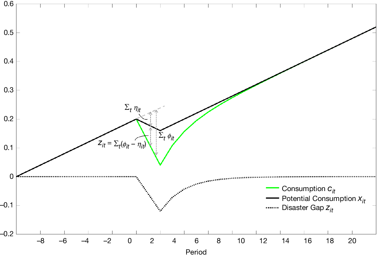
By decomposing consumption into potential consumption and a disaster gap, the model captures disaster dynamics that unfold over multiple periods and are followed by recovery. Figure 3 illustrates a typical scenario our model can generate. For simplicity, we abstract from all shocks except
 $ {\phi}_{it} $
and
 $ {\eta}_{it} $
, assume a 2% annual consumption growth trend, and simulate a two-period disaster with parameters
 $ {\rho}_z=0.6 $
,
 $ {\phi}_{it}=-0.1 $
, and
 $ {\eta}_{it}=-0.04 $
during each disaster period.
Figure 3 illustrates the evolution of consumption components during and after a simulated two-period disaster. The solid black line represents potential consumption (
 $ {x}_{it} $
), the solid green line represents actual consumption (
 $ {c}_{it} $
), and the dotted black line represents the disaster gap (
 $ {z}_{it} $
). The simulation assumes a 2% annual consumption growth trend and uses parameters
 $ {\rho}_z=0.6 $
,
 $ {\phi}_{it}=-0.1 $
, and
 $ {\eta}_{it}=-0.04 $
. The disaster occurs in periods 1 and 2, followed by a recovery phase where the disaster gap gradually dissipates while the permanent loss in potential consumption persists.
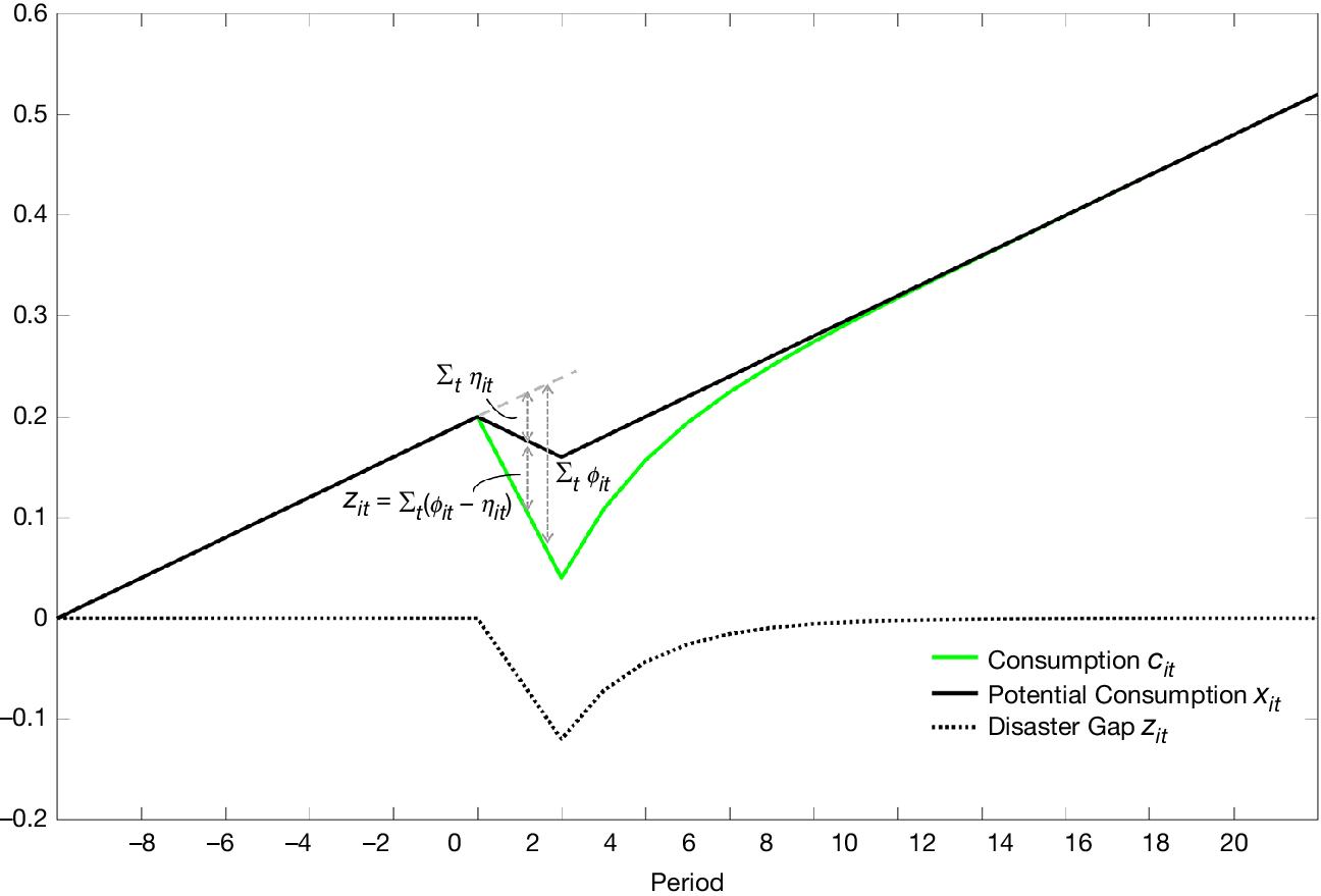
At the end of period 0, the economy enters a disaster state. Potential consumption (
 $ {x}_{it} $
, solid black line) evolves as in equation (6) and declines each period due to the persistent shock
 $ {\eta}_{it} $
, resulting in a cumulative drop of
 $ 0.08 $
, which represents the permanent damage. Actual consumption (
 $ {c}_{it} $
, green line) falls below potential consumption during the disaster. The difference between the two—the disaster gap (
 $ {z}_{it} $
)—is shown as a dotted line. It accumulates according to equation (7):
 $ {z}_{it}={z}_{i,t-1}+{\phi}_{it}-{\eta}_{it}, $
where
 $ {\phi}_{it}-{\eta}_{it} $
captures the transitory effect of the disaster.
When the disaster ends in period 2, actual consumption has cumulatively fallen by 0.2 relative to the no-disaster path. Recovery then begins. The disaster gap shrinks over time via:
 $ {z}_{it}={\rho}_z{z}_{i,t-1}, $
eventually disappearing, while the permanent loss in potential consumption (
 $ {\sum}_t{\eta}_{it}=-0.08 $
) persists. Hence, the disaster is partially permanent. The model accommodates a wide range of disaster scenarios. If
 $ {\eta}_{it}=0 $
, the disaster is fully transitory; if
 $ {\phi}_{it}={\eta}_{it} $
, the disaster is entirely permanent.
IV. Empirical Findings on Rare Disasters
A. Data
This article uses a data set on annual real per capita consumption (personal consumer expenditure) and gross domestic product (GDP) for 42 economies, which expands the Barro and Ursúa (Reference Barro and Ursúa2010) Macroeconomic Dataset, as far back as 1790 and going through 2014.Footnote 4 For most of the economies, the GDP series is longer than the corresponding consumption series. In order to fully utilize the information contained in this long-term macroeconomic data set, we concatenate the consumption and GDP series as follows: When the GDP series dates back earlier than does the corresponding consumption series, we concatenate the beginning portion of the GDP series with the corresponding consumption series.Footnote 5 For convenience, we still call the so-obtained series the consumption series, as the GDP data occur only when the corresponding consumption series are unavailable, and the main part of these series is still the consumption series. This treatment is appropriate under the assumption that the growth rates of consumption and GDP are close to each other, and helps to employ more information contained in the data, which is especially important for the study of rare disasters.
The concatenated consumption and GDP series have 6,189 country-year observations, as we choose to start from 1833 with at least ten countries. To better utilize the rich information in the data set, we allow for some short interruptions in the series, rather than discarding the beginning portion to get a shortened uninterrupted series as in Nakamura et al. (Reference Nakamura, Steinsson, Barro and Ursúa2013) and Barro and Jin (Reference Barro and Jin2021).Footnote 6 This is another reason why the data used in this study can further date back to as early as 1833.
B. Estimation Method
We use a standard Bayesian MCMC to estimate the model. This method is appropriate for complicated models like the one we have here. Moreover, we are facing data irregularities as we have unbalanced panel data with missing observations, which makes Bayesian MCMC the ideal choice for empirical implementation. Specifically, we utilize a Gibbs sampler to draw samples from the posterior distributions of the parameters and unobserved quantities, augmented with Metropolis steps when necessary (see Gelman, Carlin, Stern, Dunson, Vehtari, and Rubin (Reference Gelman, Carlin, Stern, Dunson, Vehtari and Rubin2013) for a detailed discussion on the MCMC algorithms). A more detailed explanation of this algorithm can be found in Supplementary Material Section C.
The convergence of the MCMC simulation is guaranteed under very mild conditions. In order to accurately estimate parameters and unknown quantities, we run four simulation chains with over-dispersed starting points throughout the parameter space (see Supplementary Material Section F for details on the specification of the four simulation chains). Besides visually evaluating the trace plots of parameters and unknown quantities from the simulation, we also assess the convergence by comparing the variation “between” and “within” simulated sequences (see Chapter 11 of Gelman et al. (Reference Gelman, Carlin, Stern, Dunson, Vehtari and Rubin2013) for a discussion of this method).
After 200,000 iterations, the simulation results from the four sets of far-apart initial values stabilize and become very close to each other. Therefore, we iterate each chain for 1 million times and use the latter half to analyze the posterior distributions of parameters and unknown quantities of interest. The first 500,000 iterations are dropped as burn-in.
In order to implement the Bayesian MCMC method, we need to specify various priors. In general, the priors are specified to be “not very informative.” That is, the standard deviation of the prior distribution is set to be fairly large if the prior is not flat. The detailed specification for prior distributions of parameters is listed in Table 1 in Supplementary Material Section D. We also specify the conditional prior distributions for accurate estimation. Please see Supplementary Material Sections E and F for details on these technical treatments.
C. Empirical Results
1. Time-Varying Disaster Probabilities
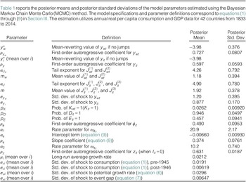
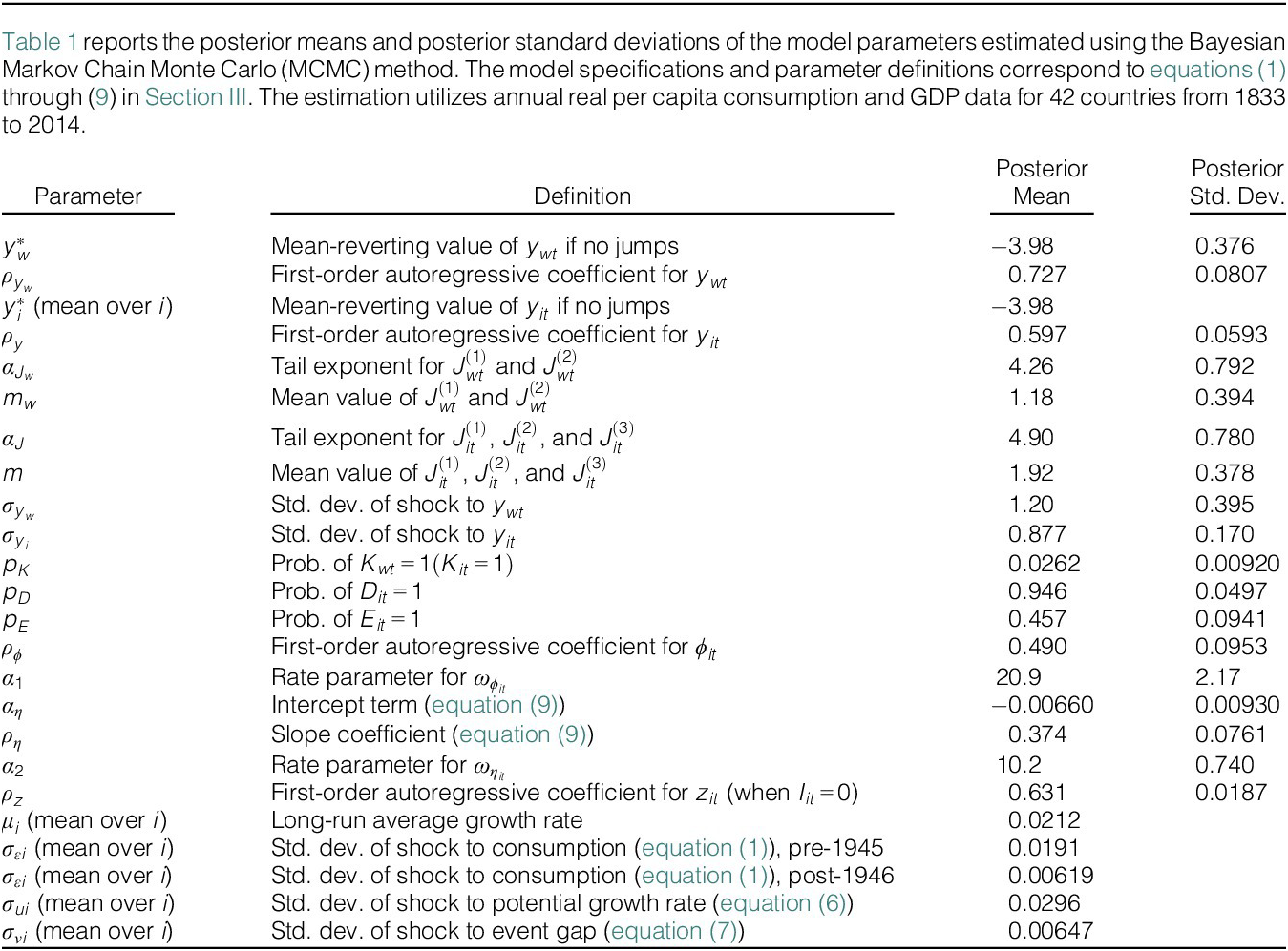
Table 1 exhibits the posterior means and standard deviations for the parameters of the model. The first group of parameters corresponds to those in equations (3) and (5) for the world and country-specific disaster indices, respectively. These indices can be converted into corresponding probability according to equations (2) and (4). Parameters
 $ {y}_w^{\ast } $
and
 $ {y}_i^{\ast } $
are the mean-reverting values of the probability indices
 $ {y}_{wt} $
for the world and
 $ {y}_{it} $
for country
 $ i $
, respectively, if there are no jumps. The posterior means of
 $ {y}_w^{\ast } $
and
 $ {y}_i^{\ast } $
(mean over
 $ i $
) are both
 $ -3.98 $
, which corresponds to a disaster probability of 1.83% per year. The process of
 $ {y}_{wt} $
is more persistent than that of
 $ {y}_{it} $
, and the posterior means of
 $ {\rho}_{y_w} $
and
 $ {\rho}_y $
are 0.727 and 0.597, respectively. Parameters
 $ {\alpha}_{J_w} $
,
 $ {m}_w $
,
 $ {\alpha}_J $
, and
 $ m $
characterize the two-sided power-law distribution of jumps in the processes of
 $ {y}_{wt} $
and
 $ {y}_{it} $
, respectively. These jumps have a mean value of 1.18 (for
 $ {J}_{wt}^{\left(\cdot \right)} $
) and 1.92 (for
 $ {J}_{it}^{\left(\cdot \right)} $
) with fat tails. According to the functional forms of the two-sided power law, the standard deviations of jumps are 0.700 (for
 $ {J}_{wt}^{\left(\cdot \right)} $
) and 0.365 (for
 $ {J}_{it}^{\left(\cdot \right)} $
). Parameter
 $ {p}_K $
characterizes the probability that an unexpected jump occurs in the processes of
 $ {y}_{wt} $
and
 $ {y}_{it} $
in a given year, and that probability is 2.62%. The posterior mean of
 $ {p}_D $
is 0.946, meaning that a world disaster at time
 $ t $
will trigger a jump in
 $ {y}_{it} $
for country
 $ i $
with very high probability. While the posterior mean of
 $ {p}_E $
is only 0.457, indicating that a previous-period country-specific disaster will trigger a jump in
 $ {y}_{it} $
for country
 $ i $
with a probability a bit less than one half. From the above analysis, we see that a worldwide disaster is more likely to continue than a country-specific disaster. Simulations using the posterior means of the parameters show that the average duration is 2.11 years for world disasters and 1.95 years for country-specific disasters.
The time-varying probability processes determine the average fractions of disaster periods for the world and an individual country in the long run. We simulate the world economy for 1 million periods using the aforementioned posterior means of the parameters, and the results indicate that the world is in the disaster state for 12.2% of the time and an individual country is in the disaster state for 12.0% of the time. Accordingly, the simulated sequences of
 $ {p}_{wt}\left(=F\left({y}_{wt}\right)\right) $
and
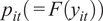 $ {p}_{it}\left(=F\left({y}_{it}\right)\right) $
have mean values of 0.122 and 0.120, respectively. On the other hand, the posterior means of
 $ {I}_{wt} $
,
 $ {I}_{it} $
,
 $ {p}_{wt} $
, and
 $ {p}_{it} $
in the MCMC are 0.117, 0.121, 0.117, and 0.119, respectively, which are very close to the corresponding statistics for the simulated world economy. We compare these statistics with the data used in Barro and Jin (Reference Barro and Jin2011), and they are very close.Footnote
7
The posterior means of the world disaster probability
 $ {p}_{wt} $
are plotted in Figure 2. The probability exceeds 25% for 22 of the 182 sample years (from 1833 to 2014): 1838–1839, 1913–1921, 1930–1933, and 1939–1945. Especially in some of these years (1914–1916, 1931, and 1940–1944), the posterior probability exceeds 50%. These years correspond to the main world disasters in the long-term international data: World War I, the Great Depression, and World War II, with the possible addition of the Great Influenza Epidemic of 1918–1920.
Figure 1 depicts our estimates of disaster probabilities for the United States and replicates the implied disaster probabilities represented in Figure 8 in Wachter (Reference Wachter2013) and in Panel A of Figure 1 in Barro and Liao (Reference Barro and Liao2021) as comparisons. In Wachter’s (Reference Wachter2013) calculation, the highest disaster probability occurs in 1920 with a value of 14%. The second-highest value occurs in 1932 with a value of 12.5%. It seems not to be a coincidence that our estimates also show two peaks in 1920 and 1932, which most likely correspond to the aftermath of World War I and the Great Depression, respectively. However, our estimated disaster probability values are much higher (
 $ >0.6 $
). There is another peak in Wachter’s (Reference Wachter2013) estimates in 1982 with a value of 10.8%, which is even higher than the disaster probability for the WWII period. Meanwhile, our estimated disaster probabilities are very small for the early 1980s, with a value of 2%, and we do not identify any disaster or event that might significantly lower the consumption during that period. Based on the comparisons between our estimated disaster probability and the real-world data used in Barro and Jin (Reference Barro and Jin2011), we think our estimates are more accurate than Wachter’s (Reference Wachter2013).Footnote
8 On the other hand, the highest value in Barro and Liao’s (Reference Barro and Liao2021) estimates of disaster probabilities for 1994–2018 is 42.5% in 2008. We also find a small peak in 2009, but the value is only 4%. As option prices can be affected by many factors, we think that some financial market risk other than real consumption disaster risk may be contributing to their empirical calculation, which makes the estimates of the disaster probability a bit too high for the 2008 financial crisis.
From Figure 2, we can also pin down years with world disaster probability between 10% and 25%. They are 1836–1837, 1840–1849, 1852–1862, 1912 (pre-WWI), 1922–1923 (post-WWI), 1928–1929 (pre-Great Depression), 1934 (post-Great Depression), 1936–1938 (pre-WWII), and 1946–1947 (post-WWII). The recent global financial crisis during 2008–2010 does not register in the figure as a worldwide disaster, with the posterior disaster probability around 3%, but it shows up as a country-specific disaster for Greece and Iceland.
We also plot the posterior means of disaster probability
 $ {p}_{it} $
for each country, which can be found in Supplementary Material Section H. It is not surprising to see that the posterior mean of
 $ {p}_{it} $
is high when the world is in a disaster. Outside of the main world disaster periods (1838–1839, 1913–1921, 1930–1933, and 1939–1945), the cases in which individual countries have posterior means for
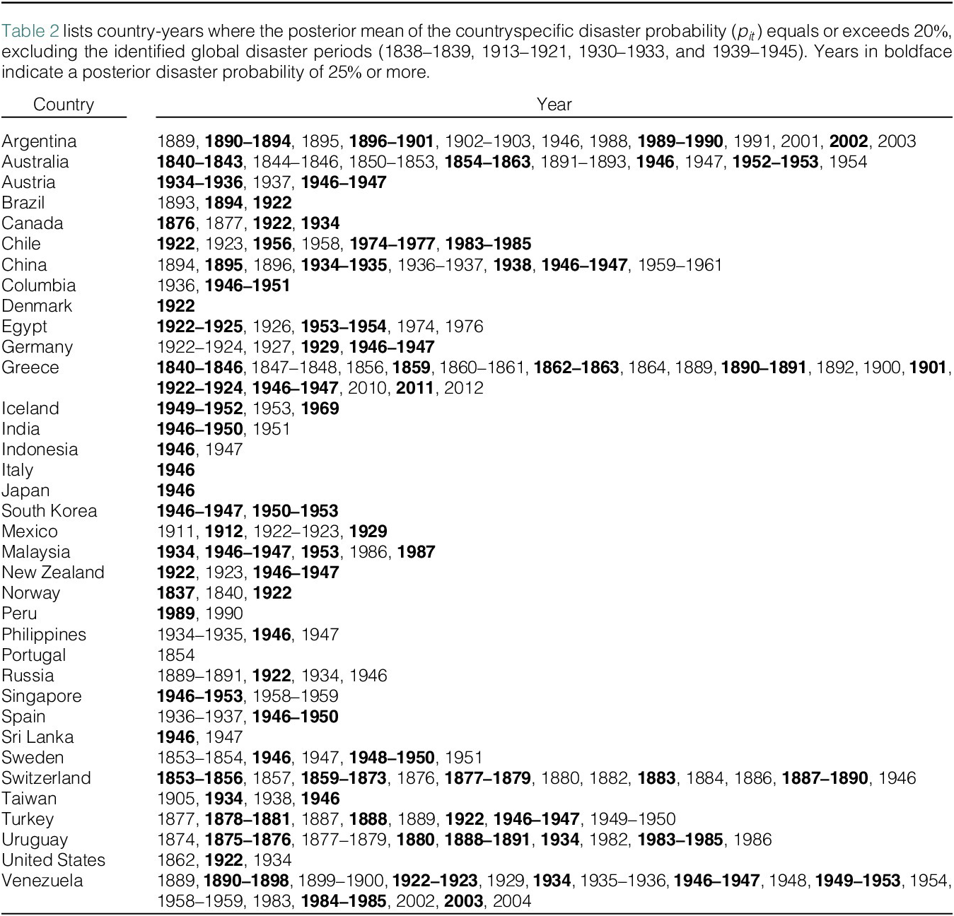
 $ {p}_{it} $
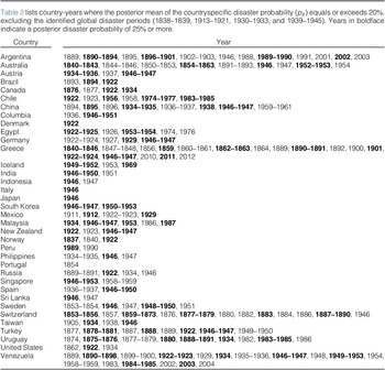
of 25% or more are listed in Table 2. These events include the Argentinean stagnation and hyperinflation in 1988–1991, the collapse of the Argentinean fixed-dollar regime in 2001–2002, the 1973 Chilean coup and its aftermath, the First Sino-Japanese War for China in 1895, the Egyptian revolution and independence as the Kingdom of Egypt in 1919–1922, the July Revolution of Egypt in 1952, the government-debt crisis and recession in Greece during 2010–2012, Indian independence in 1947, the Korean War for South Korea during 1950–1953, the violence and economic collapse in Peru in 1989–1990, the Russian Revolution and civil war during 1917–1922, and the Russo-Turkish War for Turkey in 1877–1881. Moreover, if we look into cases in which individual countries have posterior means of
 $ {p}_{it} $
between 20% and 25%, some other events will register, including China’s Great Famine during 1959–1961, the German hyperinflation in 1922–1924, the Spanish Civil War in 1936–1937, and the American Civil War in 1862.
2. Size Distribution of Disasters
The second group of parameters in Table 1 characterizes the immediate and permanent effects of disasters, along with the dynamics of disaster gaps described in equations (7)–(9). The parameter
 $ {\rho}_z=0.631 $
governs the persistence of the disaster gap, implying that over 60% of a temporary disaster shock remains after 1 year, and about 90% dissipates within 5 years. While the temporary component
 $ {\phi}_{it}-{\eta}_{it} $
eventually fades out, the long-term consequence depends on the realization of the permanent component,
 $ {\eta}_{it} $
.
In contrast to the previous rare-disaster models, where the immediate and permanent effects of a disaster are usually assumed to follow IID normal or truncated normal distributions, we allow for correlations within and between these two effects. The immediate effect
 $ {\phi}_{it} $
of a disaster evolves according to equation (8). The parameter
 $ {\rho}_{\phi } $
describes the temporal correlation between
 $ {\phi}_{it} $
and
 $ {\phi}_{i,t-1} $
. The estimated value 0.49 implies that there is a rather large serial correlation in the process of
 $ {\phi}_{it} $
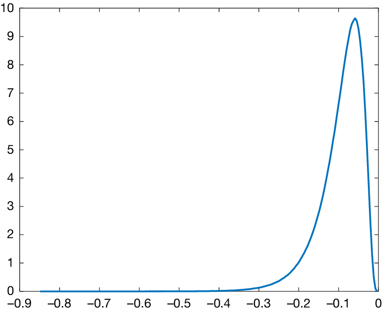
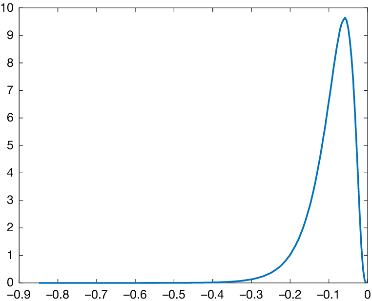
. The probability density function for
 $ {\phi}_{it} $
plotted in Figure 4 has a heavy tail on its support
 $ \left(-\infty, 0\right] $
. The simulated mean of
 $ {\phi}_{it} $
is
 $ -0.094 $
; that is, the per capita consumption falls by 9.0% on average over the first year of a disaster.Footnote
9 The simulated standard deviation of
 $ {\phi}_{it} $
is 0.055, indicating considerable dispersion in the distribution of the first-year disaster size. The probability of
 $ {\phi}_{it} $
falling below
 $ -0.149 $
log points (
 $ \approx -13.8\% $
, 1 standard deviation away from the mean) is 13.3%, and the probability of falling below
 $ -0.203 $
log points (
 $ \approx -18.4\% $
, 2 standard deviations away from the mean) is 4.7%. The probability density of the distribution of
 $ {\phi}_{it} $
diminishes exponentially, as
 $ {\phi}_{it} $
gets further away to the left, the left tail of the distribution of
 $ {\phi}_{it} $
is notably heavy. See also the discussion in footnote 3.
Figure 4 displays the simulated probability density function for the immediate disaster effect
 $ {\phi}_{it} $
. The distribution is derived from the estimated model parameters, where
 $ {\phi}_{it} $
follows an autoregressive process with error terms following an exponential distribution (see equation (8)).
For the permanent effect
 $ {\eta}_{it} $
, we allow for contemporaneous correlation with
 $ {\phi}_{it} $
, justified by the empirical link between short-run damage and long-run impact. The posterior mean of
 $ {\rho}_{\eta } $
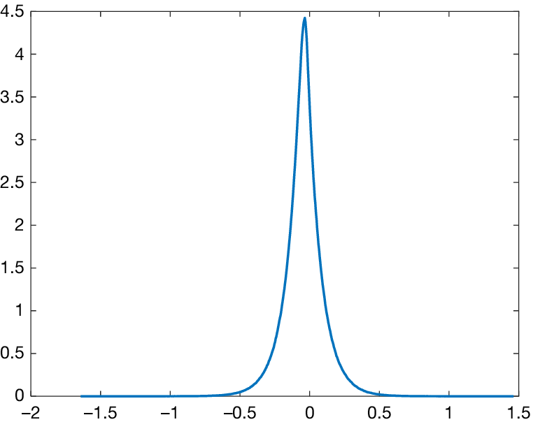
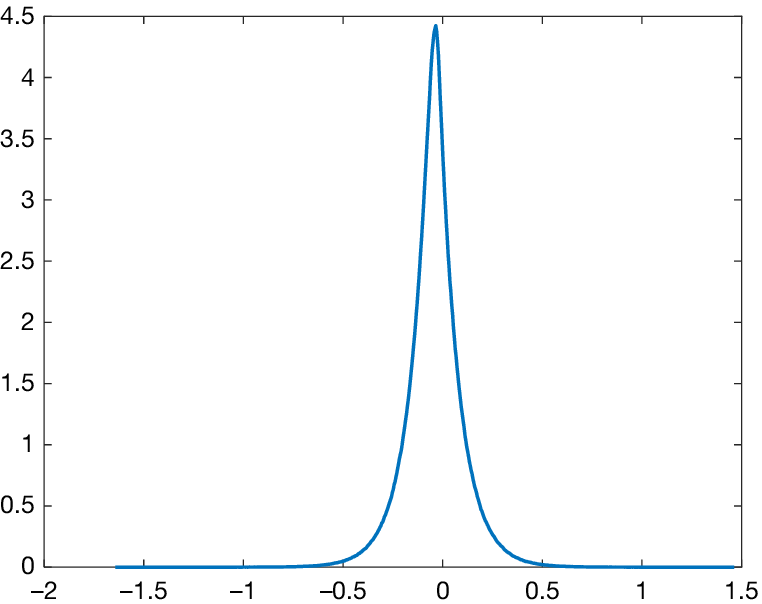
is 0.374, implying a sizable positive correlation. Figure 5 displays the slightly asymmetric distribution of
 $ {\eta}_{it} $
(due to dependence on
 $ {\phi}_{it} $
), with a simulated mean of
 $ -0.042 $
and a large standard deviation of 0.14.
Figure 5 displays the simulated probability density function for the permanent disaster effect
 $ {\eta}_{it} $
. The variable
 $ {\eta}_{it} $
determines the long-run impact of a disaster on potential consumption and is modeled to be correlated with the immediate effect
 $ {\phi}_{it} $
as specified in equation (9).
Following Barro and Ursúa (Reference Barro and Ursúa2008), we define disaster size as the peak-to-trough drop in consumption. Simulations reveal that the average disaster size is
 $ -12.2\% $
, and the standard deviation is as large as 12.8%.Footnote
10 When conditioning on disasters with peak-to-trough contractions of at least 10%, then the average disaster size is
 $ -22.1\% $
, and the standard deviation becomes 13.3%. Thus, the estimated disaster sizes in this study are extremely close to those documented in Barro and Ursúa (Reference Barro and Ursúa2008) and Barro and Jin (Reference Barro and Jin2011).Footnote
11
Our simulation indicates that, on average, 55.5% of consumption will recover over the years after disasters. That is, on average, 44.5% of the drop from the consumption trend during a disaster is permanent. Interestingly, 31.3% of disasters lead to over-recovery, where post-disaster consumption exceeds the pre-disaster trend—possibly reflecting long-run “cleansing” effects of crises.
D. Six Illustrated Countries
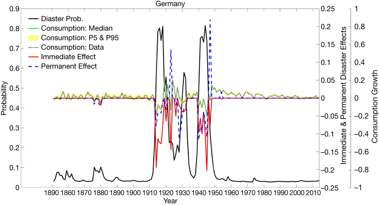
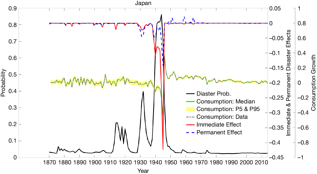
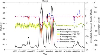
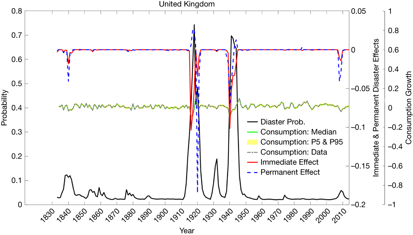
To provide a more intuitive and vivid illustration of our empirical findings, we highlight six countries: China, Germany, Japan, Russia, the United Kingdom, and the United States. Figures 6–11 display the time evolution of the posterior means of three key variables for each country: the disaster probability (
 $ {p}_{it} $
), the immediate effect (
 $ {I}_{it}{\phi}_{it} $
), and the permanent effect (
 $ {I}_{it}{\eta}_{it} $
), all expressed as quantities per year. The posterior distribution of consumption growth is also shown in each figure. The graphs clearly identify World War I, the Great Depression, and World War II as major disasters across countries. Disaster shocks—both immediate and permanent—tend to occur when the posterior mean of
 $ {p}_{it} $
is elevated, with substantial cross-country variation in their magnitude during these periods.
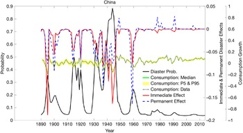
Figure 6 presents the time evolution of the key model variables for China. The solid black line plots the posterior mean of the disaster probability (
 $ {p}_{it} $
, left axis). The solid red line and dashed blue line represent the posterior means of the immediate disaster effect (
 $ {I}_{it}{\phi}_{it} $
) and permanent disaster effect (
 $ {I}_{it}{\eta}_{it} $
), respectively (right axis). The solid green line shows the median of the model-implied consumption growth, with the yellow shaded area indicating the 5th to 95th percentile confidence interval. The black dashed line represents the actual historical consumption growth data.
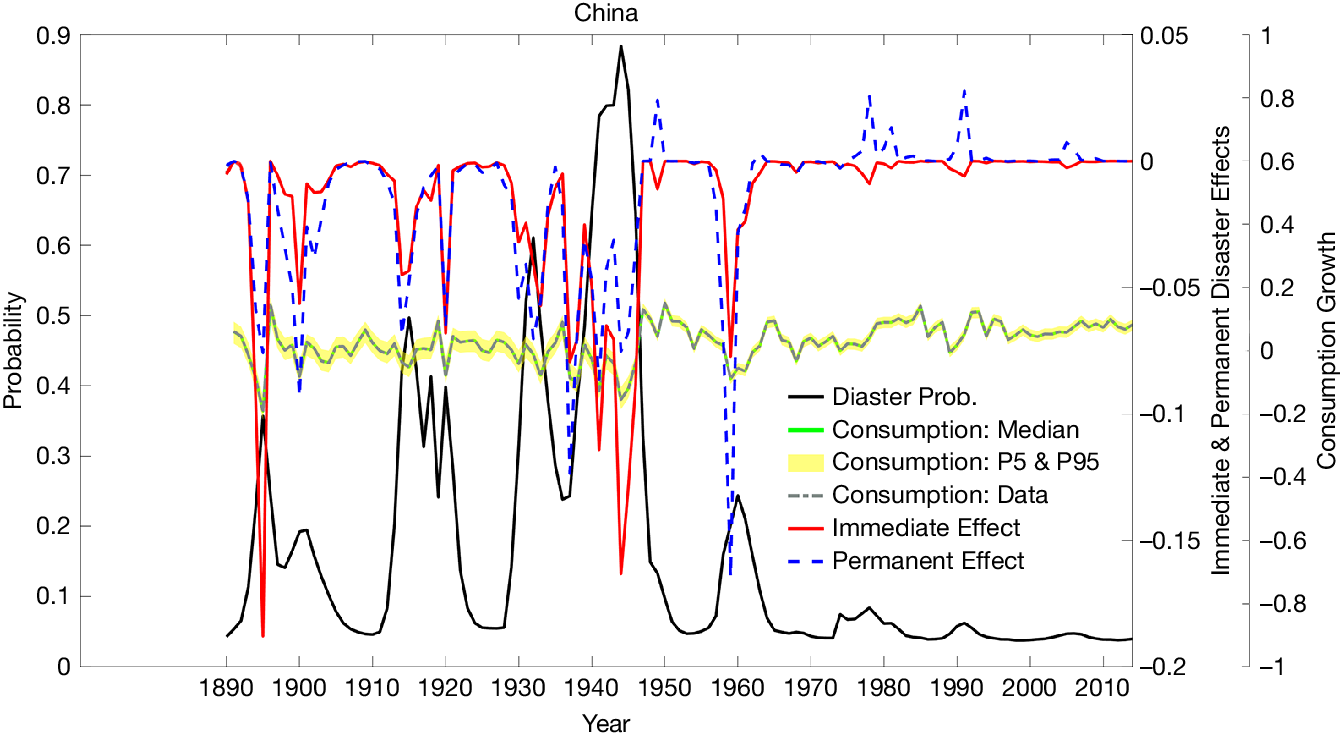
For China in Figure 6, the most severe disasters are WWII, the Great Depression, and WWI, while the First Sino-Japanese War in 1895 and the Great Chinese Famine in 1960 also register prominent disaster probabilities. The immediate disaster effect reached
 $ -17.1\% $
in 1895 and
 $ -15.1\% $
in 1944. Surprisingly or not, the permanent disaster effect was as large as
 $ -15.2\% $
in 1959 at the start of the Great Chinese Famine. For Germany in Figure 7, the disaster probability peaked during the two world wars, and the two largest immediate disaster effects were about
 $ -18\% $
both during these periods. The case for Japan in Figure 8 is similar—WWII caused the largest drop in the country’s per capita consumption level, and the immediate disaster effect was
 $ -34.5\% $
. The main disasters for Russia in Figure 9 are the two world wars, and the immediate disaster effects reached tremendously low levels of
 $ -33.8\% $
in WWII and
 $ -27.4\% $
in WWI. For the United Kingdom in Figure 10 and the United States in Figure 11, the patterns are similar but in much smaller magnitudes. The largest immediate disaster effects for these two countries are both less than 10%. However, the United Kingdom experienced a sudden drop in its long-run consumption level after WWI (
 $ -16.9\% $
in 1920), and the United States also experienced a 13.4% fall in its long-run consumption trend during the American Civil War (1861–1865).
Figure 7 presents the time evolution of the key model variables for Germany. The solid black line plots the posterior mean of the disaster probability (
 $ {p}_{it} $
, left axis). The solid red line and dashed blue line represent the posterior means of the immediate disaster effect (
 $ {I}_{it}{\phi}_{it} $
) and permanent disaster effect (
 $ {I}_{it}{\eta}_{it} $
), respectively (right axis). The solid green line shows the median of the model-implied consumption growth, with the yellow shaded area indicating the 5th to 95th percentile confidence interval. The black dashed line represents the actual historical consumption growth data.
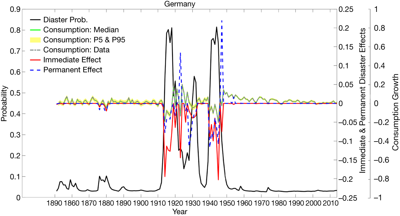
Figure 8 presents the time evolution of the key model variables for Japan. The solid black line plots the posterior mean of the disaster probability (
 $ {p}_{it} $
, left axis). The solid red line and dashed blue line represent the posterior means of the immediate disaster effect (
 $ {I}_{it}{\phi}_{it} $
) and permanent disaster effect (
 $ {I}_{it}{\eta}_{it} $
), respectively (right axis). The solid green line shows the median of the model-implied consumption growth, with the yellow shaded area indicating the 5th to 95th percentile confidence interval. The black dashed line represents the actual historical consumption growth data.
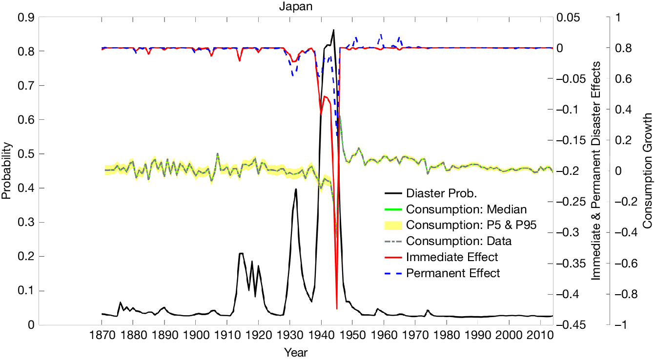
Figure 9 presents the time evolution of the key model variables for Russia. The solid black line plots the posterior mean of the disaster probability (
 $ {p}_{it} $
, left axis). The solid red line and dashed blue line represent the posterior means of the immediate disaster effect (
 $ {I}_{it}{\phi}_{it} $
) and permanent disaster effect (
 $ {I}_{it}{\eta}_{it} $
), respectively (right axis). The solid green line shows the median of the model-implied consumption growth, with the yellow shaded area indicating the 5th to 95th percentile confidence interval. The black dashed line represents the actual historical consumption growth data.
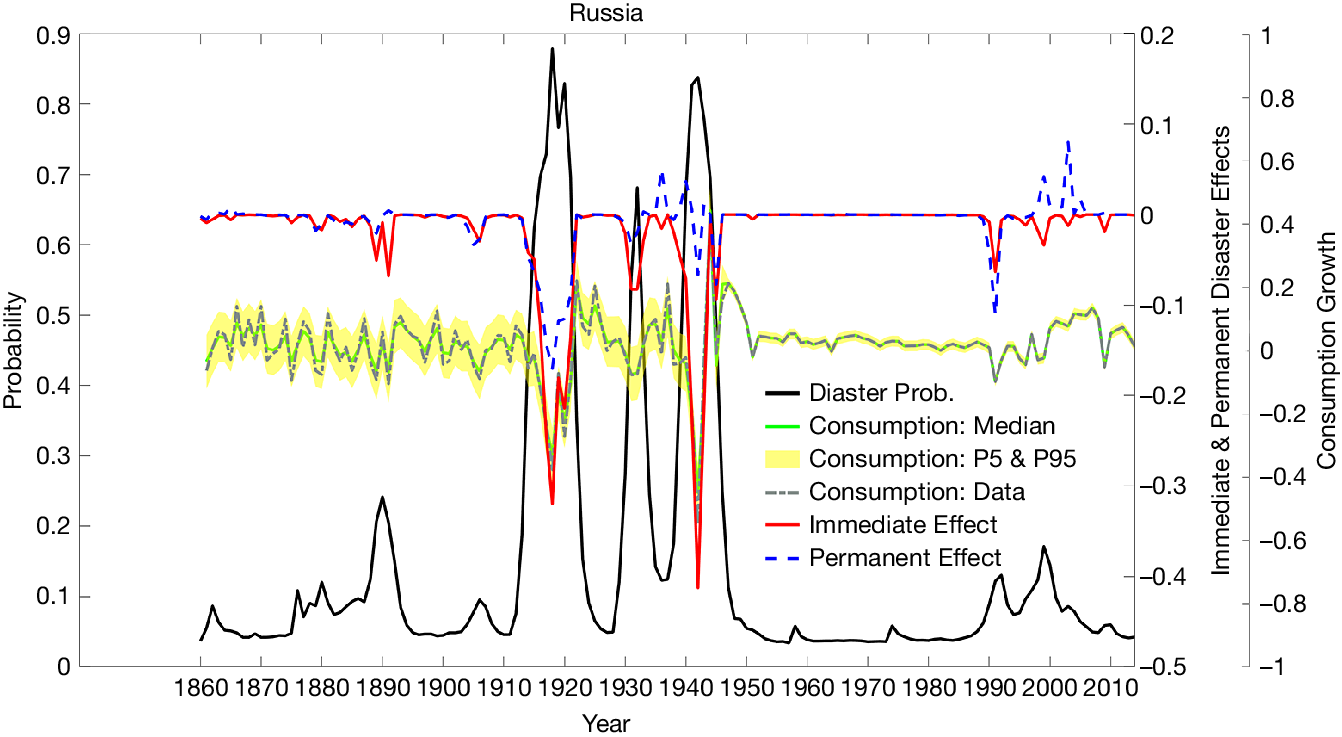
Figure 10 presents the time evolution of the key model variables for the United Kingdom. The solid black line plots the posterior mean of the disaster probability (
 $ {p}_{it} $
, left axis). The solid red line and dashed blue line represent the posterior means of the immediate disaster effect (
 $ {I}_{it}{\phi}_{it} $
) and permanent disaster effect (
 $ {I}_{it}{\eta}_{it} $
), respectively (right axis). The solid green line shows the median of the model-implied consumption growth, with the yellow shaded area indicating the 5th to 95th percentile confidence interval. The black dashed line represents the actual historical consumption growth data.
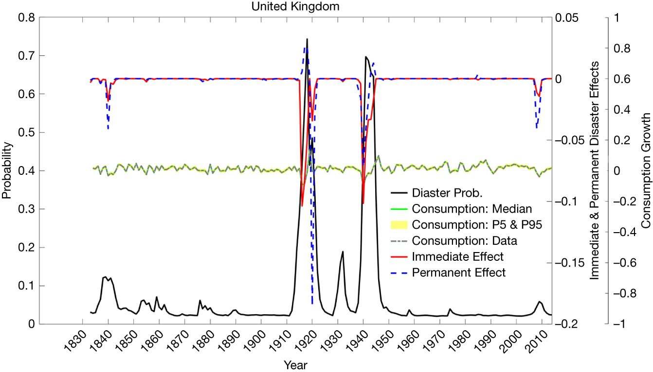
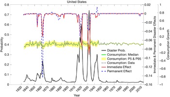
Figure 11 presents the time evolution of the key model variables for the United States. The solid black line plots the posterior mean of the disaster probability (
 $ {p}_{it} $
, left axis). The solid red line and dashed blue line represent the posterior means of the immediate disaster effect (
 $ {I}_{it}{\phi}_{it} $
) and permanent disaster effect (
 $ {I}_{it}{\eta}_{it} $
), respectively (right axis). The solid green line shows the median of the model-implied consumption growth, with the yellow shaded area indicating the 5th to 95th percentile confidence interval. The black dashed line represents the actual historical consumption growth data.
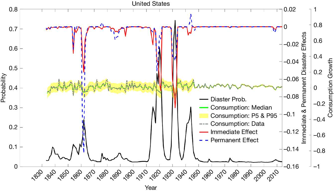
Unlike the findings in Nakamura et al. (Reference Nakamura, Steinsson, Barro and Ursúa2013) and Barro and Jin (Reference Barro and Jin2021), our results show clear persistence in both the immediate and permanent disaster effects, with fewer erratic jumps during disaster periods. This smoother pattern arises from our modified disaster dynamics in equation (7), which links the disaster gap to its own history and contemporaneous shocks. In addition, the allowance for serial correlation in
 $ {\phi}_{it} $
and its correlation with
 $ {\eta}_{it} $
leads to a more realistic characterization of disaster effects.
E. Robustness
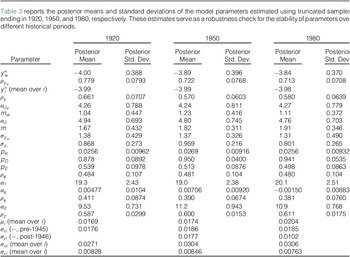
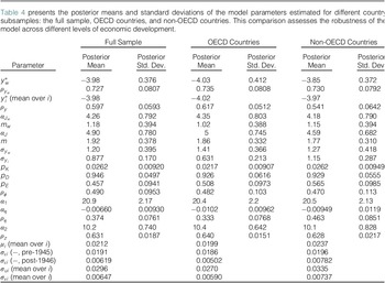
To assess the robustness of model parameters, we re-estimate the model using different subsamples across time and country groups. The results are summarized in Tables 3 and 4.
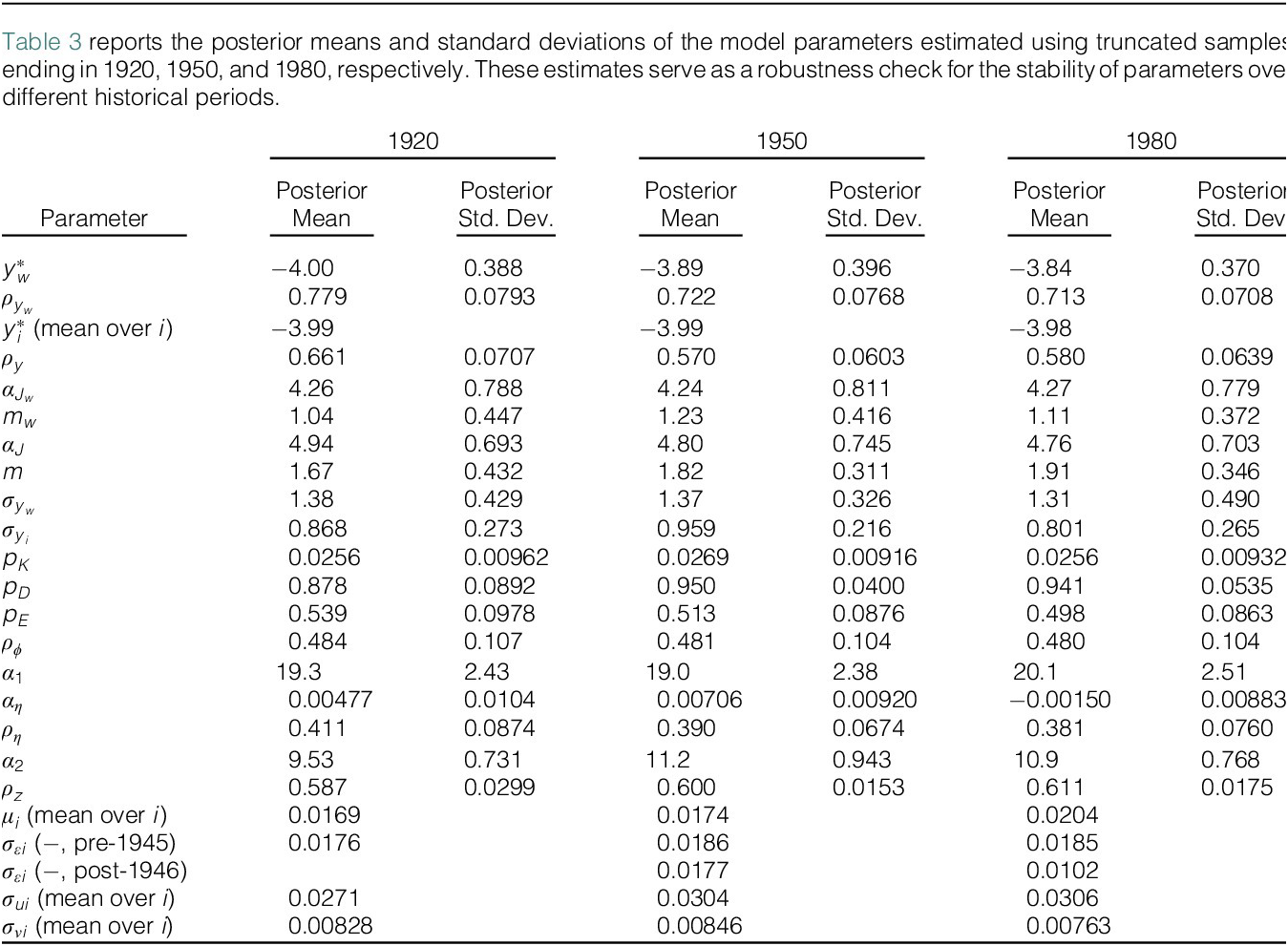
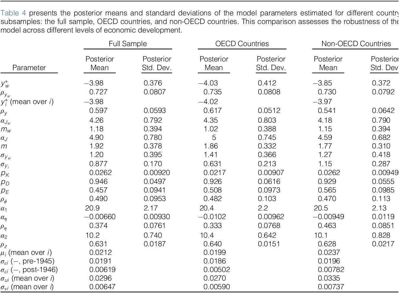
Table 3 reports estimates based on truncated time samples ending in 1920, 1950, and 1980, with the full-sample estimates (from Table 1) serving as the baseline. Parameter estimates remain broadly consistent across different sample periods in terms of posterior means and standard deviations. Slight deviations appear in the early-period sample (ending in 1920), where
 $ {\rho}_y $
is higher, and both
 $ {P}_D $
and
 $ {\rho}_z $
are lower compared with the baseline. This reflects more persistent disaster probabilities, less frequent jumps, and faster recoveries—likely due to the exclusion of several major global disasters in the early sample.
Table 4 reports results for Organization for Economic Cooperation and Development (OECD) and non-OECD groups, alongside the full sample for comparison. The parameters are generally robust across country groups, though some heterogeneity is evident. In particular, non-OECD countries display lower
 $ {\rho}_y $
and higher
 $ {\sigma}_{yi} $
, indicating more volatile and less persistent disaster probabilities. They also exhibit larger standard deviations in volatility-related parameters—
 $ {\sigma}_{\unicode{x025B}_i} $
,
 $ {\sigma}_{u_i} $
, and
 $ {\sigma}_{\mu_i} $
—as well as higher
 $ {\rho}_{\eta } $
, suggesting that disasters tend to have more severe and lasting effects in these economies.
V. Asset Pricing
A. Framework
We now analyze the asset-pricing implications of the estimated consumption disaster model and discuss the effects on asset prices from the disentanglement of disaster probability and the realization of disasters. We assume that the representative agent in the endowment economy has Epstein and Zin (Reference Epstein and Zin1989) and Weil (Reference Weil1990) (EZW) preferences. Under these preferences, Epstein and Zin (Reference Epstein and Zin1989) show that the return on any asset satisfies the condition
 $$ {\unicode{x1D53C}}_t\left[{\beta}^{\frac{1-\gamma }{1-\theta }}{\left(\frac{C_{t+1}}{C_t}\right)}^{\frac{-\theta \left(1-\gamma \right)}{1-\theta }}{R}_{w,t+1}^{\frac{\theta -\gamma }{1-\theta }}{R}_{a,t+1}\right]=1, $$
where
 $ {R}_{a,t+1} $
denotes the gross return on asset a from period
 $ t $
to
 $ t+1 $
and
 $ {R}_{w,t+1} $
is the gross return on total wealth, which in our model equals the value of the equity claim on a country’s consumption. The parameter
 $ \beta $
is the subjective discount factor,
 $ \gamma $
is the coefficient of relative risk aversion, and
 $ \frac{1}{\theta } $
is the intertemporal elasticity of substitution (IES), which governs the agent’s desire to smooth consumption over time. The EZW preferences delink the CRRA and the IES and avoid some counterintuitive predictions in asset pricing that a power utility function would make.
The Euler condition for asset return, equation (10), cannot be solved analytically. Hence, we adopt a standard numerical method. Specifically, equation (10) is an integral equation for the price-dividend ratio of the consumption claim. We can find the fixed point of the corresponding function via iteration. Given the price-dividend ratio of the consumption claim, the pricing of other assets can be determined by solving equation (10).Footnote 12
The values of
 $ \gamma $
and
 $ \beta $
are estimated by matching the observed long-term average real rates of return on corporate equity and short-term government bills—a proxy for risk-free claims. There are long-history data for 17 countries in Barro and Ursúa ((Reference Barro and Ursúa2008), Table 5),Footnote
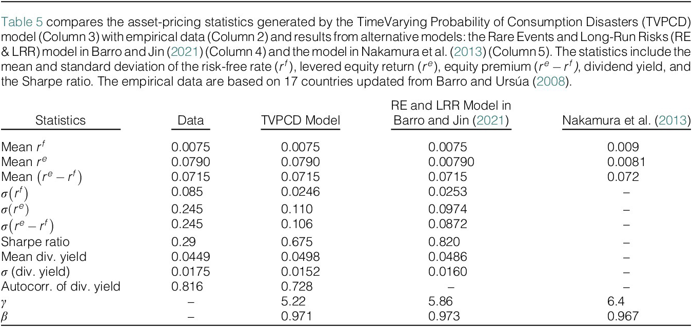
13 which we update to 2014. The arithmetic average of real rates of return is 7.9% per year on levered equity and 0.75% per year on short-term government bills (see column 2 of Table 5). Hence, the average equity premium is 7.15% per year. As the data on equity returns are observations of levered claims on the consumption stream, we assume a corporate debt–equity ratio of 0.5, following Nakamura et al. (Reference Nakamura, Steinsson, Barro and Ursúa2013).
Besides the dynamics model parameters listed in Table 1, the values of CRRA (
 $ \gamma $
), IES (
 $ \frac{1}{\theta } $
), and the subjective discount factor (
 $ \beta $
) need to be determined to analyze the asset-pricing implications of the estimated disaster model. There has been a debate over the appropriate value for the IES in the macroeconomics and finance literature. Bansal and Yaron (Reference Bansal and Yaron2004) claim that an IES greater than 1 is critical for capturing the “reasonable” positive relationship between the expected consumption growth rate and the price-dividend ratio for an unlevered equity claim on consumption. Barro (Reference Barro2009) also notes that IES
 $ >1 $
is necessary for a negative relationship between the consumption uncertainty and this price-dividend ratio. Moreover, Nakamura et al. (Reference Nakamura, Steinsson, Barro and Ursúa2013) show that low IES values, such as IES
 $ \le 1 $
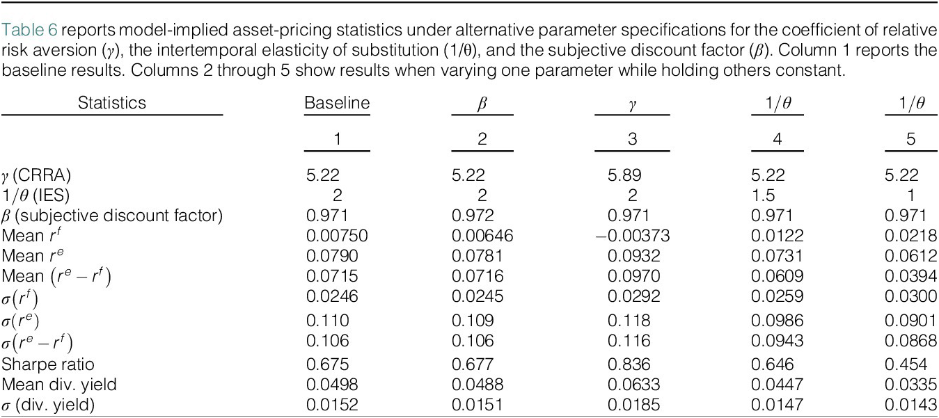
, are inconsistent with the observed behavior of asset prices during consumption disasters. Bansal and Yaron (Reference Bansal and Yaron2004) use a value of 1.5, and Barro (Reference Barro2009), Barro and Jin (Reference Barro and Jin2021), and Nakamura et al. (Reference Nakamura, Steinsson, Barro and Ursúa2013) adopt Gruber’s (Reference Gruber2013) empirical estimate of 2. Since our model is based on the framework established by Nakamura et al. (Reference Nakamura, Steinsson, Barro and Ursúa2013), we also use IES = 2 for comparability. We also explore the impact of varying IES values on asset-pricing outcomes in Table 6. Next, we determine the values of two free parameters,
 $ \gamma $
and
 $ \beta $
, to fit the observed long-term average real rates of return on corporate equity and short-term government bills.
B. Empirical Evaluation
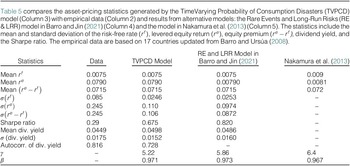
The asset-pricing results are exhibited in Table 5. The second column reports the target empirical values of various asset-pricing statistics, including the mean and standard deviation of the risk-free rate
 $ {r}^f $
, the levered equity return
 $ {r}^e $
, and the equity premium
 $ {r}^e-{r}^f $
; the Sharpe ratio; and the mean and standard deviation of the dividend yield. These statistics are obtained from Barro and Ursúa (Reference Barro and Ursúa2008) and Global Financial Data.
The asset-pricing results are summarized in Table 5. Column 2 reports the empirical targets, including the mean and standard deviation of the risk-free rate (
 $ {r}^f $
), equity return (
 $ {r}^e $
), equity premium (
 $ {r}^e-{r}^f $
), Sharpe ratio, and dividend yield, sourced from Barro and Ursúa (Reference Barro and Ursúa2008) and Global Financial Data. Column 3 presents results from our baseline TVPCD model, whereas columns 4 and 5 report corresponding outcomes from the RE & LRR (Rare events and long-run risks)model in Barro and Jin (Reference Barro and Jin2021) and the Nakamura et al. (Reference Nakamura, Steinsson, Barro and Ursúa2013) model, respectively.
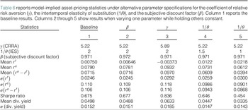
Given an IES of 2 and the parameter estimates in Table 1, both the TVPCD and RE & LRR models match the observed average risk-free rate (0.75%) and equity premium (7.15%). The required CRRA is 5.2 for our model, compared with 5.9 in the RE & LRR model and 6.4 in Nakamura et al. (Reference Nakamura, Steinsson, Barro and Ursúa2013). The reduction in the required risk aversion stems primarily from the time-varying nature of disaster probabilities, which allows the model to generate risk premia even in the absence of realized disasters. Additional features—such as persistence in immediate effects and their correlation with permanent damage—further enhance the model’s ability to capture asset-pricing moments.
In terms of volatility, our model estimates
 $ \sigma \left({r}^e-{r}^f\right)=0.106 $
and a Sharpe ratio of 0.675, which exceeds the empirical benchmark of 0.29. While the volatility is still underestimated, the result is reasonable, given the model’s general equilibrium structure and a conservative debt–equity ratio of 0.5. For comparison, Barro and Jin (Reference Barro and Jin2021) report
 $ \sigma \left({r}^e-{r}^f\right)=0.087 $
with
 $ \gamma =5.9 $
. Notably, as reported in Table 6, asset return volatilities increase with
 $ \gamma $
, and the introduction of time-varying disaster risk significantly amplifies the model-implied volatility of equity premia. Consequently, the TVPCD model delivers a more realistic Sharpe ratio than the RE & LRR benchmark.Footnote
14 Similarly, our model produces a higher and more plausible estimate of equity return volatility
 $ \sigma \left({r}^e\right) $
.
Our model estimates an average dividend yield of 4.98% with a volatility of 1.52%, both broadly consistent with empirical observations. However, the first-order autocorrelation of dividend yield is 0.728, lower than the empirical value of approximately 0.816. This discrepancy stems from the fact that our model does not target dividend yield—or any asset price moments—during estimation. In addition, dividends are modeled as a fixed proportion of consumption under the assumption of a low corporate debt-to-equity ratio (0.5), without explicitly modeling the dividend process. Similar simplifications are also discussed in Marfè and Pénasse (Reference Marfè and Pénasse2024).
We also explore the sensitivity of asset-pricing results to variations in the subjective discount factor
 $ \beta $
, the risk aversion coefficient
 $ \gamma $
, and the IES, as reported in Table 6. Increasing
 $ \beta $
lowers both the mean risk-free rate and the mean equity return, with a slightly larger effect on the former, leading to a modest rise in the average equity premium. At the same time, volatilities of asset returns and dividend yield decline slightly, whereas the Sharpe ratio increases. Raising
 $ \gamma $
reduces the mean risk-free rate and increases the equity return, thus widening the equity premium. Other asset-pricing moments, such as volatilities and the Sharpe ratio, also increase. Finally, decreasing the IES to 1.5 or 1 raises the mean risk-free rate and lowers the equity return, resulting in a smaller equity premium. In these cases, the volatility of the risk-free rate rises, whereas other asset-pricing statistics fall relative to the benchmark.
We next discuss the model’s implications for excess return and consumption predictability. Numerous studies (e.g., Campbell and Shiller (Reference Campbell and Shiller1988), Cochrane (Reference Cochrane1992), Fama and French (Reference Fama and French1989), and Keim and Stambaugh (Reference Keim and Stambaugh1986)) have shown that high dividend yields predict high excess returns. Therefore, I conducted the following panel regression analysis to examine whether the dividend yield in the model can predict excess stock returns:
 $$ \frac{1}{H}\sum \limits_{h=1}^H\left[\mathit{\log}\left({R}_{i,t+h}^e\right)-\mathit{\log}\left({R}_{i,t+h}^b\right)\right]={\alpha}_i+\beta {divyield}_{it}+{\unicode{x025B}}_{i,t+H}, $$
where
 $ {R}_{i,t+h}^e $
and
 $ {R}_{i,t+h}^b $
are, respectively, country
 $ i $
’s return on aggregate market and on government bill between
 $ t+h-1 $
and
 $ t+h $
, and
 $ {divyield}_{i,t} $
is country
 $ i $
’s dividend yield on the aggregate market at period
 $ t $
.
To facilitate comparison, I performed the regression using both historical data and simulated data from the model. The historical data are drawn from 17 countries with long data histories (as detailed in Table 5, see footnote 13), starting from 1920.Footnote 15 To ensure that the statistical power of the model-based regression is as close as possible to that of the historical data, we simulated 1,000 paths for 17 economies, each with a length of 1,000 years, and performed a panel regression on each simulated path. We calculate this regression for returns measured over horizons ranging from 1 to 10 years.
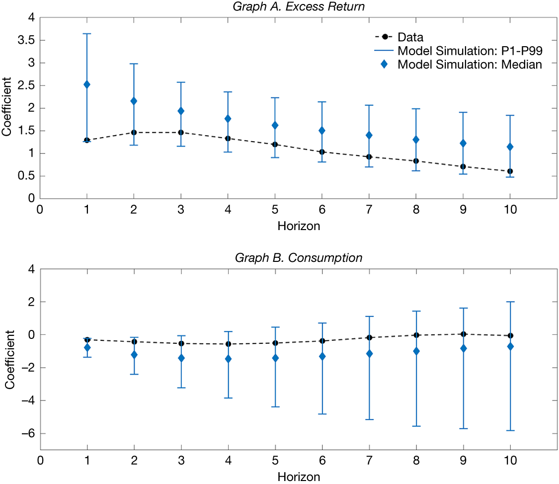
Graph A of Figure 12 presents the 1st, 50th, and 99th percentiles of the predictive coefficients from the model simulations, alongside their empirical counterparts. The positive distribution of coefficients for dividend yield across all horizons indicates that our model effectively captures the equity premium predictability of the dividend yield observed in the data. As observed in the trend of the regression coefficients, there is a gradual decline in the magnitude of these coefficients as the prediction horizon lengthens. This long-term downward trend in coefficient values is consistent with the implications of our model and is also observed in other studies on rare disasters.Footnote 16 As is typical in models with time-varying disaster probabilities, disaster risk tends to mean-revert, with the risk premium and dividend yield reverting along with it. Consequently, periods of high disaster risk are generally followed by periods of relatively lower disaster risk. Therefore, as the forecast horizon extends, the coefficient estimate is expected to decline. Graph A of Figure 12 also shows the empirical counterparts. The point estimates of the regression coefficients exhibit a similar pattern and fall within the interval produced by the model simulations at each horizon. Although there is a slight uptick in empirical coefficients at shorter horizons—likely a result of data noise—the overall trend aligns with the model’s projections, exhibiting a downward trajectory as the forecast horizon lengthens.
Figure 12 evaluates the model’s ability to reproduce the empirical long-horizon predictability of excess stock returns and consumption growth by the dividend yield. Graph A displays the slope coefficients from panel regressions of cumulative excess stock returns on the initial dividend yield over horizons ranging from 1 to 10 years (equation (11)). Graph B displays the coefficients from panel regressions of cumulative consumption growth on the dividend yield (equation (12)). The black dots represent point estimates from historical data (17 countries, post-1920). The blue diamonds represent the median estimates from 1,000 model simulations, with error bars indicating the 1st to 99th percentile range.

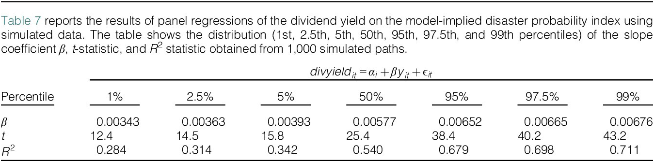
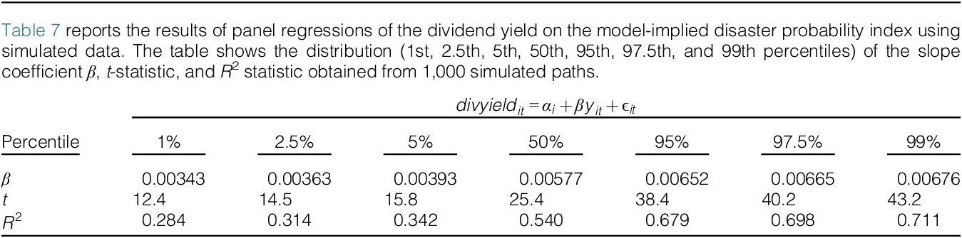
This finding of predictability follows naturally from our model’s properties: A high dividend yield is associated with elevated disaster risk, which in turn predicts higher future expected returns on stocks relative to bonds. Table 7 presents the regression results of the dividend yield on the disaster probability index derived from the model simulations. We report various percentiles of the coefficient estimates, standard errors, and
 $ {R}^2 $
statistics. The median
 $ {R}^2 $
exceeds 0.5, indicating that the fear of potential disasters significantly drives the variation in dividend yield. An elevated probability of disaster drives up the dividend yield, which in turn signals higher expected future excess returns on stocks. Therefore, fluctuations in disaster probability could potentially serve as a predictor of future stock excess returns, a topic we examine further in Section VI.
It is also valuable to examine the extent of consumption growth predictability implied by the model. Similar to the previous analysis, we conduct predictive panel regressions of H-year-ahead log consumption growth on past country dividend yields:
 $$ \sum \limits_{h=1}^H\Delta {c}_{i,t+h}={\alpha}_i+\beta {divyield}_{i,t}+{\unicode{x025B}}_{i,t+H}, $$
where
 $ \Delta {c}_{i,t+h} $
is country
 $ i $
’s log growth in aggregate consumption between periods
 $ t+h-1 $
and
 $ t+h $
, and
 $ {divyield}_{i,t} $
is country
 $ i $
’s dividend yield on the aggregate market at period
 $ t $
.
Graph B of Figure 12 shows the estimation results for cumulative horizons ranging from 1 to 10 years. The coefficients from the simulated data vary widely, with both positive and negative values for each horizon, indicating insignificant evidence of consumption growth predictability. The point estimates from the historical data exhibit a similar pattern, with magnitudes close to 0. These findings align with several studies (e.g., Beeler and Campbell (Reference Beeler and Campbell2012), Campbell (Reference Campbell2003), Cochrane (Reference Cochrane1994), Hall (Reference Hall1988), Lettau and Ludvigson (Reference Lettau and Ludvigson2001)) that also report little to no predictability of consumption growth over long horizons.
VI. Predictability from Disaster Probability Index
A. Model-Implied Predictability
From the analysis in Section V, we understand that the disaster probability index could serve as a predictor for future stock excess returns. In this section, we will conduct a deeper analysis of this possibility. We will begin by examining the model’s implications on the predictability of the disaster probability index.
We utilize the following panel regression model to investigate the predictability of future excess returns:
 $$ \frac{1}{H}\sum \limits_{h=1}^H\left[\mathit{\log}\left({R}_{i,t+h}^e\right)-\mathit{\log}\left({R}_{i,t+h}^b\right)\right]={\alpha}_i+\beta {y}_{it}+{\unicode{x025B}}_{i,t+H}, $$
where
 $ {R}_{i,t+h}^e $
and
 $ {R}_{i,t+h}^b $
are the gross returns on aggregate stock market indices and short-term government bills from year
 $ \left(t+h-1\right) $
to year
 $ \left(t+h\right) $
for country
 $ i $
, respectively,
 $ H $
is the forecasting horizon,
 $ {y}_{it} $
is the disaster probability index of country
 $ i $
, and
 $ {\mu}_i $
accounts for the country fixed effects. We conduct this regression analysis using data generated through simulations. As in Section V, we simulated 1,000 paths for 17 different economies, each spanning 1,000 years, and ran a panel regression on each simulated path. This analysis was carried out for returns measured over various time horizons, ranging from 1 to 10 years.
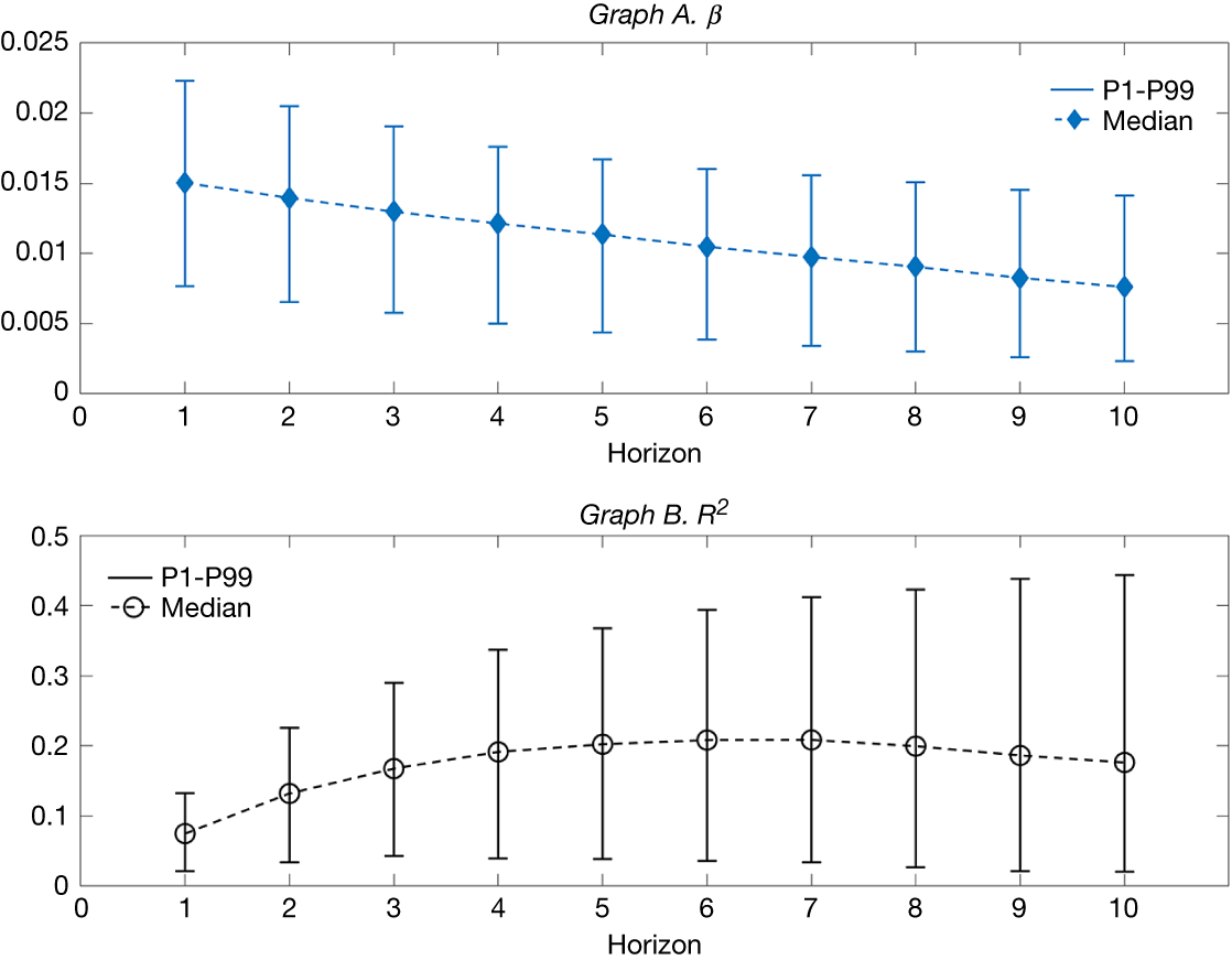
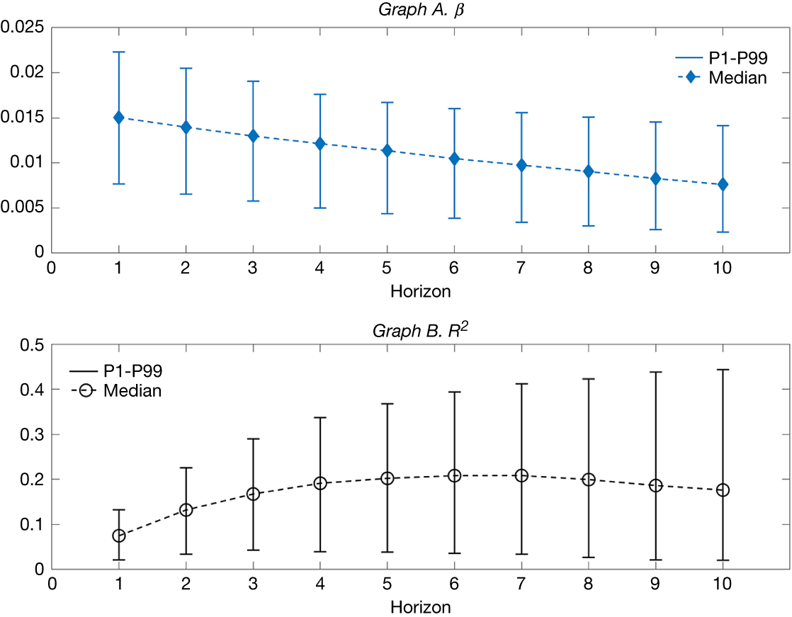
Graph A of Figure 13 presents the 1st, 50th, and 99th percentiles of the predictive coefficients derived from the regressions of simulated data. The results indicate a robust positive relationship between the disaster probability index and excess returns across all forecast horizons, underscoring the influence of disaster risk on stock returns. As the forecast horizon extends, we observe a gradual decrease in the magnitude of these coefficients, reflecting a diminishing impact of disaster probability on excess returns over time. This pattern is consistent with the characteristics of a disaster model with time-varying probabilities, where disaster risk tends to mean-revert—an issue we have already discussed in Section V.B. Graph B of Figure 13 displays the
 $ {R}^2 $
values from these regressions, showing a clear upward trend as the forecast horizon extends. The
 $ {R}^2 $
starts at 0.075 for a 1-year horizon and reaches a peak of 0.208 around the seventh year, followed by a slight decline. This initial rise in
 $ {R}^2 $
likely reflects the reduction in noise from short-term returns as the horizon lengthens, allowing for clearer predictive signals. However, as the forecast horizon becomes too extended, the
 $ {R}^2 $
experiences a modest drop, indicating a diminishing predictive power over the longer term.
Figure 13 illustrates the predictive power of the disaster probability index for excess stock returns based on model simulations. Graph A plots the distribution (median and 1st–99th percentiles) of the slope coefficients (
 $ \beta $
) from panel regressions of cumulative excess returns on the disaster probability index
 $ {y}_{it} $
over horizons of 1 to 10 years (equation (13)). Graph B plots the corresponding distribution of the R
2 statistics.
B. Real-Time Return Predictability
The model simulation results in Section VI.A confirm the significant predictive power of the disaster probability index on future excess returns. In this section, we evaluate the real-time predictability of the empirical disaster probability index. For this end, we regress the average future excess stock return on the posterior mean of the country disaster probability index estimated from the TVPCD model. The panel regression model used here is identical to the regression model (13) in Section VI.A, but with
 $ {y}_{it} $
and
 $ \log \left({R}_{i,t+h}^e\right)-\log \left({R}_{i,t+h}^b\right) $
derived from historical data rather than model simulations. Additionally, to ensure real-time prediction, each period’s estimate of the disaster probability index
 $ {y}_{it} $
relies solely on the information available up to each point in time.
Specifically,
 $ {y}_{it} $
represents the contemporaneous posterior mean of country
 $ i $
’s disaster probability index. We construct
 $ {y}_{it} $
in real time using an expanding-window approach. For each year
 $ t $
, we estimate
 $ {y}_{it} $
based on data available from the sample’s starting year (1833) up to year
 $ t $
. We rerun the MCMC estimation procedure to obtain the posterior mean of country
 $ i $
’s disaster probability index
 $ {y}_{it} $
using all available data up to period
 $ t $
. This process is repeated for subsequent years
 $ t+1 $
,
 $ t+2 $
, and so on, using all the data available up to those years. We then use this real-time disaster probability index
 $ {y}_{it} $
to forecast future equity premiums over horizons ranging from 1 to 10 years. Given that some countries in the sample have later start dates for their consumption data, the real-time estimates of
 $ {y}_{it} $
start from 1920.
Panel A of Table 8 presents the predictive regression results using the full sample period across forecasting horizons of 1 to 10 years. The results reveal that the disaster probability index is a strong predictor of future returns. Specifically, a one-unit increase in the disaster probability index (equivalent to a 5.5 percentage point rise in the disaster probability, based on the sample average of disaster probability index) predicts a 0.91 percentage point higher return in the following year, with the predicted premium rising to 3.1% annually over a 3-year horizon. The magnitude of the regression coefficients initially experiences a slight increase in the short term, followed by a gradual decrease as the forecast horizon extends, while maintaining consistent predictive significance. The early rise in coefficients may be attributed to the presence of more noise in the short-horizon return data. Additionally, the
 $ {R}^2 $
statistic shows a steady upward trend as the forecast horizon lengthens, reaching nearly 3.3% at the 10-year mark. Compared with the regression results from the simulated data in Section VI.A, the
 $ {R}^2 $
from the real-time prediction regressions are considerably lower. This discrepancy is likely due to the greater variation in actual return data, which includes more shocks beyond disaster risk.
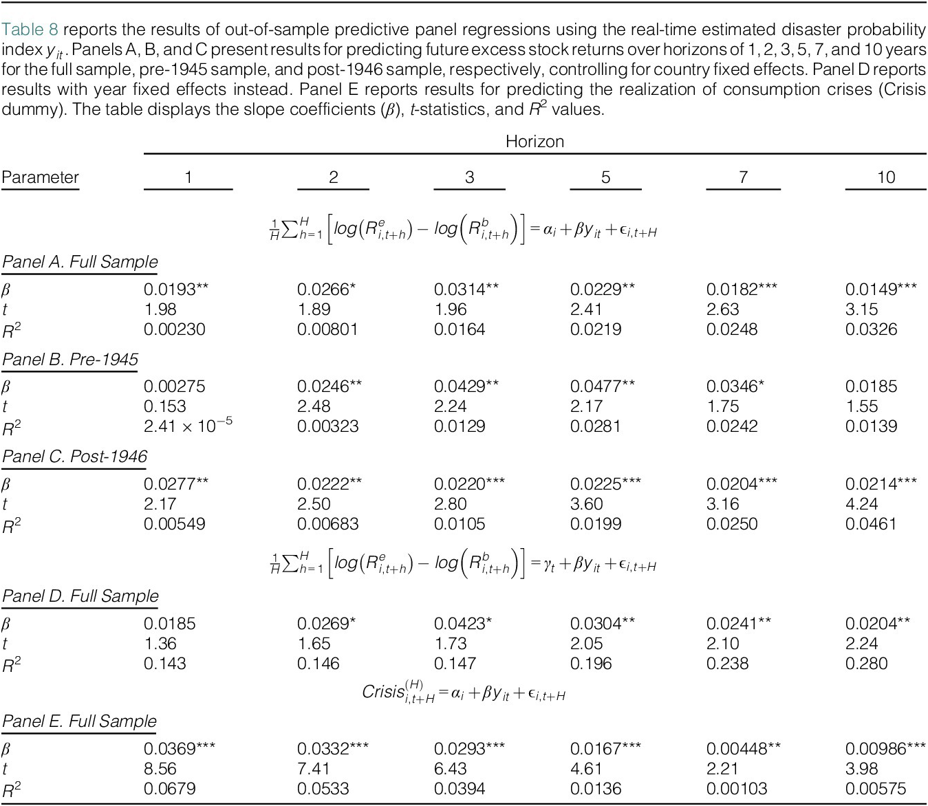
Turning to the subperiods, Panels B and C of Table 8 report the prediction results for the prewar (pre-1945) and postwar (post-1946) periods. One notable difference between these two periods is that far fewer disasters occurred in the latter. Despite this, we see that even in the postwar era, the disaster probability index continues to exhibit strong and sustained predictive power. Manela and Moreira (Reference Manela and Moreira2017) interpret this postwar predictability as being driven by ongoing concerns about potential disasters.
To explore whether disaster risk has cross-sectional predictability for returns, we examine the same predictability regressions, replacing country fixed effects with year fixed effects. Panel D of Table 8 presents these regression results. The coefficients become significantly positive after two periods, and their significance increases notably after five periods. The weaker significance in the earlier periods may be due to the interference of other individual-level factors, which diminish as the forecasting horizon extends. This result suggests that the disaster probability index also exhibits some predictive power at the cross-sectional level, as economies with higher disaster risk tend to predict higher future excess returns.
To further supplement the discussion on the disaster risk predictive power, we examine whether the disaster indices possess any out-of-sample forecasting power for realized disasters. Specifically, we conduct the following panel regression:
 $$ {Crisis}_{i,t+H}^{(H)}={\alpha}_i+\beta {y}_{it}+{\unicode{x025B}}_{i,t+H}. $$
Here, the dependent variable is the crisis dummy variable, which indicates whether country
 $ i $
is experiencing a disaster at time
 $ t $
. The variable
 $ Crisis=1 $
denotes the occurrence of a disaster, while
 $ Crisis=0 $
indicates otherwise. We adopt the definition from Marfè and Pénasse (Reference Marfè and Pénasse2024): A macroeconomic crisis is identified as a 2-standard-deviation decline in consumption growth relative to its long-term trajectory:
 $$ Crisi{s}_{i,t}^{(H)}=\left\{\begin{array}{cc}1,& \mathrm{if}\;\Delta {c}_{i,t}^{\left.H\right)}<\mathrm{mean}\left(\Delta {c}_{i,t}^{(H)}\right)-2\times \mathrm{SD}\left(\Delta {c}_{i,t}^{(H)}\right),\\ {}0,& \mathrm{otherwise},\end{array}\right. $$
where the H-year consumption growth is measured as
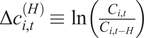 $ \Delta {c}_{i,t}^{(H)}\equiv \ln \left(\frac{C_{i,t}}{C_{i,t-H}}\right) $
.
Panel E of Table 8 presents the results of this predictive panel regression. We observe that the disaster probability index demonstrates strong forecasting power for future crises across all horizons. This finding not only reinforces the reliability of the disaster probability index but also lends some support to its predictive power for returns.
VII. Conclusions
To the best of our knowledge, this is the first article to incorporate time-varying disaster probabilities into the rare-disaster model and to estimate the physical (or “real”) processes of disasters and disaster probabilities in an integrated global framework with international interactions of disaster risks. All the parameters used to characterize the processes of disasters and disaster probabilities are estimated using the long-term national accounts data, which avoids the potential tendency of overstating the disaster risk in typical parameter calibration when using financial market data. The model identifies major historical disaster episodes, such as the world wars and the Great Depression, along with some disasters that affected only individual countries or several countries. The empirical results from the TVPCD model accord very well with historical records of macroeconomic disasters, and we think our estimates are more accurate than those reported in recent similar studies.
With respect to the asset-pricing implications of the estimated model, a match of the observed real rates of return on risk-free claims and corporate equity requires a
 $ \gamma $
of 5.2, which is substantially smaller than the estimates from previous rare-disaster models. The introduction of the time-varying disaster probability delinks the variations in disaster probabilities and the realizations of disasters, lowers the required CRRA
 $ \gamma $
, increases the estimated volatilities of equity returns and premia, and provides a better match for the Sharpe ratio compared with previous rare-disaster models. Moreover, the out-of-sample predictive regressions show that the disaster probability index estimated from our model has significant real-time predictive power for excess returns over long horizons, and this predictive ability holds both over time and in the cross section.
Financial Statement
This study is supported by the National Natural Science Foundation of China (Grant No. 72403043) and the Ministry of Education Project of Humanities and Social Sciences (Grant No. 22YJC790045).
Supplementary Material
To view supplementary material for this article, please visit http://doi.org/10.1017/S0022109025101853.