1 Introduction
Geophysical flows are well known to be strongly influenced by the density stratification at intermediate scales of the order of
 $1{-}100~\text{m}$
in the ocean and
 $100{-}1000~\text{m}$
in the atmosphere (see, e.g. Thorpe Reference Thorpe2005). This stratification is often used to decouple the horizontal quasi-geostrophic motions from the non-geostrophic internal waves (Riley & Lelong Reference Riley and Lelong2000) in order to simplify the dynamics of the flow. However, the coupling between these two types of motion is a subtle phenomenon which is still deeply studied, especially in the case of turbulent flows (Thorpe Reference Thorpe2016). A generic example of such a decaying turbulent flow is the bluff body wake in a continuously stratified fluid, which has been studied for more than 50 years (Lin & Pao Reference Lin and Pao1979; Baines Reference Baines1987; Spedding Reference Spedding2014) due to its fundamental interest and geophysical applications. The goal of this paper is to give quantitative predictions of the internal waves emitted by a horizontally translating bluff body using a detailed comparison between experimental results and theoretical models.
Theoretically, the solution of a moving point source in a stratified fluid has been known since the early pioneering paper of Lighthill (Reference Lighthill1967) on anisotropic waves. The phase lines of these lee waves can be easily computed and were compared successfully with experimental measurements on the translation of a steady cylinder (Stevenson Reference Stevenson1968; Boyer et al. Reference Boyer, Davies, Fernando and Zhang1989), an oscillating cylinder (Stevenson & Thomas Reference Stevenson and Thomas1969) and a tilted cylinder (Meunier Reference Meunier2012). The amplitude of the internal waves was later given as a complex analytical series by Miles (Reference Miles1968) and approximated in the far field by Miles (Reference Miles1971) using the stationary phase method. This solution has been generalized using Green’s functions for a time dependent fixed point source (Voisin Reference Voisin1991) and for a point source moving with a non-constant velocity (Voisin Reference Voisin1994).
The lee waves of a translating sphere have been studied experimentally in detail by Bonneton, Chomaz & Hopfinger (Reference Bonneton, Chomaz and Hopfinger1993) and Robey (Reference Robey1997). On one hand, Bonneton et al. (Reference Bonneton, Chomaz and Hopfinger1993) focused on the wake of a small sphere in a deep pycnocline (i.e. in a continuously stratified fluid of height much larger than the sphere diameter). They found that the wave isophases and the amplitude were in agreement with the prediction of Miles (Reference Miles1971) for moderate Froude numbers
 $1<F<2$
where
 $F=2U_{B}/(ND)$
(
 $U_{B}$
being the towing velocity,
 $D$
the diameter and
 $N$
the buoyancy frequency). On the other hand, Robey (Reference Robey1997) studied the wake of a large sphere in a thin thermocline where the lee waves exhibited a discrete set of eigenmodes. The isophases of these modes were in good agreement with the theoretical model based on Milder (Reference Milder1974). But the amplitude could only be correctly predicted by assuming that the streamwise length of the bluff body was three times larger than the sphere diameter. Robey (Reference Robey1997) explained that this required tuning of the model was due to the presence of the recirculation zone behind the bluff body. However this prediction was only correct for
 $F<4$
. Indeed, both experimental studies showed the presence of a second type of internal wave at smaller wavelength. These waves were emitted by the turbulent wake itself and became stronger than the lee waves for Froude numbers larger than 4 (Bonneton et al.
Reference Bonneton, Chomaz and Hopfinger1993; Robey Reference Robey1997). These wake waves will be described further on.
The Green’s function formulation of the lee waves described by Voisin (Reference Voisin1994) was extended by Scase & Dalziel (Reference Scase and Dalziel2004) to bluff bodies towed at an angle with respect to the horizontal. Their asymptotic solutions were compared to experimental results at low Froude number in Scase & Dalziel (Reference Scase and Dalziel2006), which showed that the finite size of the source and the viscous attenuation should be taken into account. The drag due to the internal waves can be derived from these formulae and has been refined by Voisin (Reference Voisin2007). These predictions have been recently compared to experimental measurements by Brandt & Rottier (Reference Brandt and Rottier2015). They found that the lee wave drag is correctly predicted at low Froude number but that it is larger than the expected value at moderate Froude (
 $2<F<5$
). They explained this discrepancy by the presence of the wake waves (despite their attempt to remove their contribution). In this paper, we will show that this discrepancy may come from an additional term in the model due to the excitation of lee waves by the drag. We will introduce this term in the model used by Robey (Reference Robey1997) and show that it is dominant at moderate Froude number.
In order to understand the generation of waves by the turbulent wake, the structure of the wake is now briefly described. At large enough Reynolds numbers (larger than a few thousands), the near wake is three-dimensional with a velocity defect decreasing as
 $t^{-2/3}$
and a wake width increasing as
 $t^{1/3}$
as in a homogeneous wake (see, e.g. Tennekes & Lumley Reference Tennekes and Lumley1972). Here, time
 $t$
corresponds to the time after the passage of the bluff body, which corresponds to a downstream distance
 $x=U_{B}t$
. At
 $Nt=2$
, the velocity defect becomes small enough such that the local Froude number (based on the velocity defect and the wake width) becomes of order unity (meaning that the Ozmidov scale becomes of the order of the wake width). Stratification starts to modify the wake with two major effects: the saturation of the wake height and the creation of flat horizontal vortices (see the review by Lin & Pao Reference Lin and Pao1979). The saturation of the wake height (together with the momentum conservation) induces a slower decay of the velocity defect as
 $t^{-0.25}$
. However, Spedding (Reference Spedding1997) showed experimentally that this stage, called the non-equilibrium (NEQ) regime, is only transient since the velocity decreases faster again after
 $Nt=50$
as
 $t^{-2/3}$
during the quasi two-dimensional regime (Spedding Reference Spedding1997; Gourlay et al.
Reference Gourlay, Arendt, Fritts and Werne2001; Dommermuth et al.
Reference Dommermuth, Rottman, Innis and Novikov2002; Diamessis, Spedding & Domaradzki Reference Diamessis, Spedding and Domaradzki2011; Pal et al.
Reference Pal, Sarkar, Posa and Balaras2017) due to the vertical diffusion of the wake (Chomaz et al.
Reference Chomaz, Bonneton, Butet and Hopfinger1993a
). Despite this complex temporal dependence of the velocity defect, the horizontal wake width and the distance between pancake vortices were found experimentally to increase as
 $t^{1/3}$
in all stages (Spedding Reference Spedding1997, Reference Spedding2002). All these temporal dependencies can be modelled by simply assuming that the vertical Reynolds stress vanishes at
 $Nt=2$
, as proposed theoretically (Meunier, Diamessis & Spedding Reference Meunier, Diamessis and Spedding2006) and confirmed numerically (Redford, Lund & Coleman Reference Redford, Lund and Coleman2015).
Waves generated by the turbulent wake were first observed by Gilreath & Brandt (Reference Gilreath and Brandt1985) behind a self-propelled body. These non-deterministic waves were thought to be generated by the collapse of the large scale turbulent bursts. Such random waves were also observed by Bonneton et al. (Reference Bonneton, Chomaz and Hopfinger1993) in the wake of a towed sphere. They formed semi-concentric waves with a short wavelength (of the order of the sphere diameter). However, Bonneton et al. (Reference Bonneton, Chomaz and Hopfinger1993) also observed coherent waves with a slightly larger wavelength (of the order of three diameters) at later times. The wavelength of these coherent waves was shown by Hopfinger et al. (Reference Hopfinger, Flor, Chomaz and Bonneton1991) and Lin, Boyer & Fernando (Reference Lin, Boyer and Fernando1993) to be equal to the vertical oscillation of the turbulent wake due to the spiral instability.
Robey (Reference Robey1997) also observed these coherent wake waves in a thin thermocline (without the random semi-concentric waves) and predicted their wavelength and amplitude by assuming that the waves were emitted by a single pancake vortex translating at the wake defect velocity. However, the theoretical spatial structure of the waves was not exactly similar to the structure obtained experimentally. It should be noted that this model is very close to the model proposed by Dupont & Voisin (Reference Dupont and Voisin1996) of a point source translating at the bluff body velocity with an oscillating frequency equal to the vortex shedding frequency.
Spedding et al. (Reference Spedding, Browand, Bell, Chen, Lawrence, Pieters and Yonemitsu2000) observed experimentally these coherent waves in a thick density stratification and showed that the wavelength scales as
 $F^{1/3}$
like the spacing of the coherent pancake vortices of the wake. The detailed numerical study of Abdilghanie & Diamessis (Reference Abdilghanie and Diamessis2013) also confirmed this dependence as
 $F^{1/3}$
. The waves are emitted as a burst during the NEQ regime, which can last until
 $Nt=50$
at moderate Reynolds numbers and until
 $Nt=100$
at larger Reynolds numbers. This increase of emitted internal waves can also be obtained by reducing the density diffusion coefficient rather than the kinematic viscosity, as shown by de Stadler, Sarkar & Brucker (Reference de Stadler, Sarkar and Brucker2010). Zhou & Diamessis (Reference Zhou and Diamessis2016) showed that the wavelength decreases as
 $t^{-1}$
far above the wake due to the dispersive nature of the wave. They also found that the wavelength decreases slightly with the Reynolds number and is correlated with the vertical Taylor scale of the wake turbulence.
A different mechanism has been identified in a turbulent vertical shear where internal waves are emitted by the spanwise Kelvin–Helmholtz billows (Munroe & Sutherland Reference Munroe and Sutherland2014). Recently, Watanabe et al. (Reference Watanabe, Riley, de Bruyn Kops, Diamessis and Zhou2016) showed that the thickness of the interface between the turbulent and the non-turbulent region scales with the Kolmogorov scale and that the loss of energy due to wave radiation and to turbulent dissipation are comparable. In this paper, we will show that the wake waves are excited by the coherent pancake vortices of the wake, as stated by Robey (Reference Robey1997). We will extend his model of internal waves emitted by a single vortex to internal waves emitted by a periodic array of vortices.
The goal of this paper is to provide extensive experimental particle image velocimetry (PIV) measurements of the internal waves emitted by a weakly stratified wake. The large amount of data obtained by this technique permits us to separate the two types of waves on a large range of Froude numbers. The characteristics of the lee waves are obtained for large Froude numbers and show that there is a missing ingredient in classical models of lee waves, due to the drag of the bluff body (i.e. to the separation of the flow behind the bluff body). We also show that the wake waves can be explained by the emission of waves by the array of coherent vortices. The paper is organized as follows. In § 2, we describe the experimental set-up and the technique used to separate the two types of waves. Section 3 is devoted to the lee waves and § 4 to the wake waves. Conclusions follow in § 5.
2 Materials and methods
The experiment has been described in detail in previous papers (Spedding, Browand & Fincham Reference Spedding, Browand and Fincham1996; Spedding Reference Spedding1997), and only the main features of the apparatus, and of the data acquisition are outlined here.
2.1 Experimental devices
A bluff body with diameter
 $D$
(equal to 1.28 cm or 2.52 cm for the sphere) is towed at a velocity
 $U_{B}$
ranging from
 $2~\text{cm}~\text{s}^{-1}$
to
 $1~\text{m}~\text{s}^{-1}$
along the
 $x$
direction. The bluff body is maintained at a height
 $z_{0}$
above the bottom of the tank by three thin wires (
 $d=250$
microns) under strong tension
 $T$
, as shown in figure 1. These tow wires slide along three guide cables with a minimum of vibration. The disturbances created by the wakes of the tow wires themselves (where
 $Re<250$
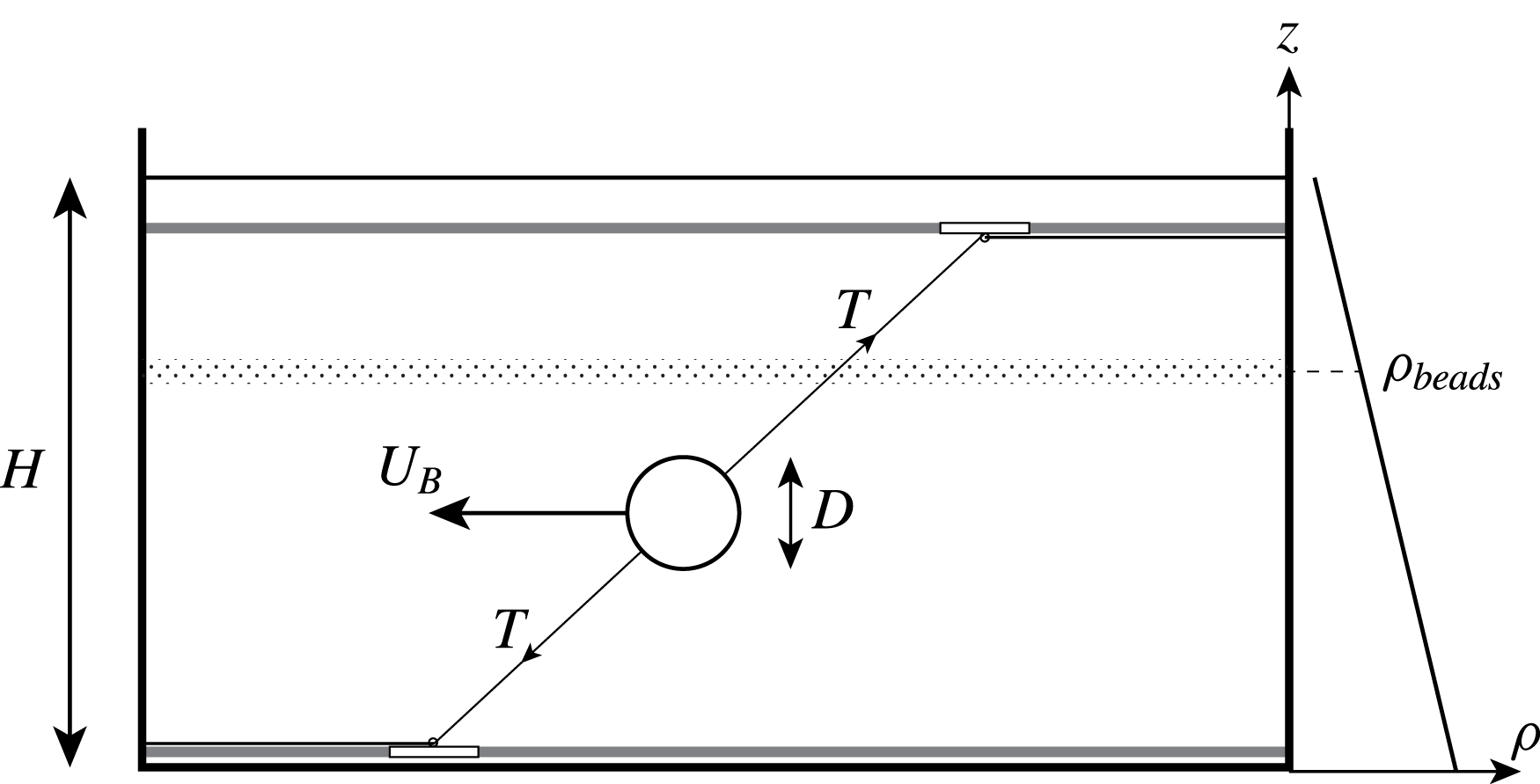
) are negligible in amplitude compared with the wake of the bluff body. Furthermore, the obliquely mounted wires do not intersect the measurement plane, which is close to the body height. To investigate the influence of the shape of the body, several objects are used: a sphere for comparison with previous results, two slender objects such as a 6 : 1 cylinder (with diameter 1.28 and 2.68 cm) and a 6 : 1 spheroid (with diameter 1.3 and 2.54 cm). Both the spheroid and the cylinder are towed in the direction of the major axis. However, most of the results are obtained for the sphere.
Schematic of the experimental set-up. The sphere of diameter
 $D$
is towed at velocity
 $U_{B}$
by thin wires with a strong tension
 $T$
.

The tank of horizontal section
 $380\times 244~\text{cm}^{2}$
is filled up to a height varying from 24 to 26 cm with stably stratified salted water using the double bucket method. The density difference, of the order of 10 %, allows us to reach a buoyancy frequency
 $N=[(-g/\unicode[STIX]{x1D70C}_{0})(\unicode[STIX]{x2202}\unicode[STIX]{x1D70C}/\unicode[STIX]{x2202}z)]^{1/2}$
of the order of
 $2~\text{s}^{-1}$
.
2.2 Parameters of the flow
Using the tow speed,
 $U_{B}$
, the diameter,
 $D$
, of the bluff body, the kinematic viscosity of the fluid
 $\unicode[STIX]{x1D708}=1.02\times 10^{-6}~\text{m}^{2}~\text{s}^{-1}$
and the buoyancy frequency
 $N$
, two non-dimensional parameters can be defined. The Reynolds number
 $Re\equiv U_{B}D/\unicode[STIX]{x1D708}$
is varied between 600 and 15 000. The Froude number defined by
 $F\equiv 2U_{B}/ND$
, where
 $N$
is the buoyancy frequency, is varied between 1 and 96, and for a set of experiments with fixed
 $N$
and
 $D$
, it is proportional to the Reynolds number.
2.3 Particle image velocimetry (PIV)
The flow is analysed by measuring horizontal two-dimensional instantaneous velocity fields using PIV. For flow seeding, small polystyrene beads are carefully sorted out with a density adjusted to within 0.15 %. When introduced in the stratified fluid, the particles settle at the specific height where the fluid has the same density marking an isopycnal with a thickness of approximately 3 mm. The height
 $z$
of the isopycnal can be moderately modified, by adding or removing small amounts of heavy fluid at the bottom of the tank, to be located at the desired altitude above the bluff body (typically 0 to 2 diameters above the centreline). The particles are illuminated by four
 $1~\text{kW}$
floodlights and their positions are recorded on a Pulnix TM9701 CCD camera positioned above the tank, over a field of view with dimensions
 $79\times 56~\text{cm}^{2}$
. The digital images are treated by a variant of the customized correlation image velocimetry (CIV) algorithm described in detail in Fincham & Spedding (Reference Fincham and Spedding1997). The resulting velocity fields correspond to the horizontal velocities
 $(u,v)$
since the camera is far above the tank (approximately 3 m). The uncertainties in the individual velocity measurements are of the order of 1 %. The vertical derivative of the vertical component of the velocity can be calculated from the incompressibility
 $\unicode[STIX]{x2202}w/\unicode[STIX]{x2202}z=-\unicode[STIX]{x2202}u/\unicode[STIX]{x2202}x-\unicode[STIX]{x2202}v/\unicode[STIX]{x2202}y$
where partial derivatives of
 $u$
and
 $v$
are calculated by a smoothing spline interpolation of the velocity field with an uncertainty of less than 10 %. This quantity is a good indicator of internal waves and is insensitive to the presence of horizontal vortices known to appear in stratified wakes. As noted earlier, the velocity fields are obtained at different times
 $t$
after the bluff body has crossed the centre of the image which correspond to downstream distances behind the bluff body equal to
 $x=U_{B}t$
at the centre of the image (also written
 $x/D=Nt~F/2$
in non-dimensional units).
2.4 Two types of internal waves
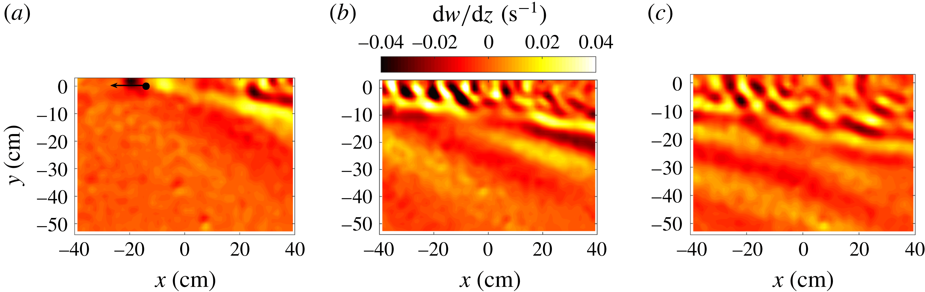
Typical instantaneous fields of vertical divergence are shown in figure 2 (the sphere being translated from right to left). They exhibit two types of internal waves at two different wavelengths. The first set of waves propagates rapidly far from the axis of the bluff body due to its large wavelength and has a small angle between the isophases and the
 $x$
-axis. The second set of waves remains closer to the
 $x$
-axis because the wavelength is smaller and has a larger angle close to
 $45^{\circ }$
between the isophases and the
 $x$
-axis.
Divergence measured two diameters above the centre of the sphere at (a)
 $Nt=2.7$
, (b)
 $Nt=21.6$
and (c)
 $Nt=40.5$
.
 $F=4$
,
 $Re=2400$
. The measurement plane is located at
 $z/H=0.629$
and the bluff body at
 $z_{0}/H=0.435$
.

These two types of internal waves were already observed by Bonneton et al. (Reference Bonneton, Chomaz and Hopfinger1993) and Robey (Reference Robey1997) who showed that the first set of waves (with large wavelength) corresponds to the lee waves of the bluff body itself with an amplitude decreasing with the Froude number. They also indicated that the second set of waves (with small wavelength) is emitted by the turbulent wake and has an amplitude increasing with the Froude number.
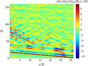
These two sets of waves have a very different phase velocity and it is convenient to use this property to separate them. This is clearly visible in the spatio-temporal diagram of figure 3 where the lee waves appear at early times (from
 $Nt=0$
to 30) and propagate very rapidly in
 $x$
. Fitting an isophase (black solid line on the figure) indicates that the slope is close to
 $2/F$
, meaning that the position increases as
 $x/D=NtF/2$
, i.e. that the lee waves have an
 $x$
-phase velocity equal to the bluff body velocity
 $U_{B}$
. By contrast, the wake waves (isophases fitted by blue solid lines) appear at later times (from
 $Nt=30$
to 150) and propagate slower in
 $x$
.
Spatio-temporal diagram measured two diameters above the centre of the sphere at
 $y=5D$
. The grey (magenta) dashed line marks an isophase of the wake waves and the black dashed line marks an isophase of the lee waves.
 $F=4$
,
 $Re=2400$
,
 $z/H=0.63$
and
 $z_{0}/H=0.44$
.

In the next section, the lee internal waves will be studied by looking at the divergence field far from the
 $x$
-axis at early times and in the frame of reference of the bluff body. The wake waves will be studied in § 4 by looking at the divergence close to the
 $x$
-axis at later times and in a frame of reference moving slowly with respect to the laboratory frame of reference.
3 Lee waves
3.1 Experimental measurements
Since the lee waves are stationary in the frame of reference moving with the bluff body, it is possible to do a temporal average in this frame of reference. This amounts to do a change of variable from
 $x$
to a new streamwise coordinate
 $X=x+U_{B}t$
. To do so, the instantaneous divergence fields are translated by a distance
 $x=U_{B}t$
and the mean field is obtained at each location
 $X$
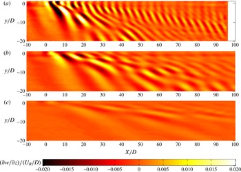
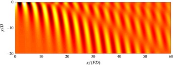
from the average of all available instantaneous divergence fields. This type of reconstruction is convenient since it removes the wake waves which are not stationary in this frame of reference. An example is given in figure 4 for three different Froude numbers. The lee waves propagate from the position of the sphere and have a complicated structure with dislocations in the isophases. These dislocations were not present in the experimental results of Bonneton et al. (Reference Bonneton, Chomaz and Hopfinger1993) probably due to the fact that the height of fluid is here smaller than in their experiments. Their results were in good agreement with the theory in an infinite fluid. Here, the presence of dislocations suggest that only a finite number of vertical Fourier modes are excited as obtained experimentally by Robey (Reference Robey1997) and explained theoretically by Vasholz (Reference Vasholz2011).
Mean vertical velocity gradient
 $\unicode[STIX]{x2202}w/\unicode[STIX]{x2202}z$
in the frame moving with the sphere measured two diameters above the centre of the sphere at (a)
 $F=1$
,
 $Re=600$
, (b)
 $F=2$
,
 $Re=1200$
and (c)
 $F=4$
,
 $Re=2400$
.
 $z/H=0.629$
and
 $z_{0}/H=0.435$
.

By comparing the divergence fields at different Froude numbers, it is clear that the wavelength (dimensionalized by
 $D$
) increases with the Froude number and that the amplitude (dimensionalized by
 $U_{B}/D$
) decreases with the Froude number. This can be quantified by extracting
 $X$
-profiles of divergence at a given position
 $y$
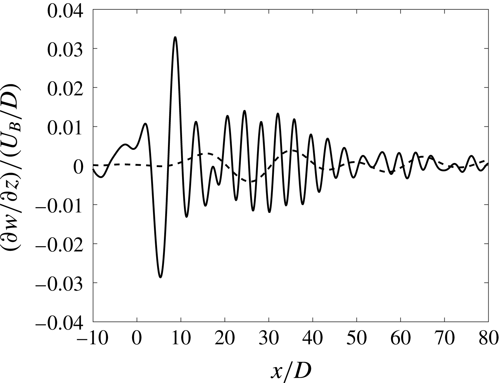
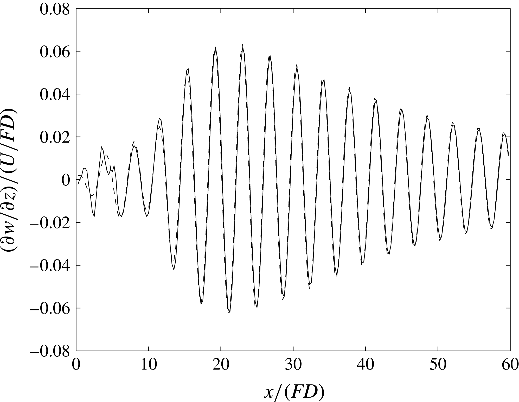
. Figure 5 shows such a profile at
 $y=-3D$
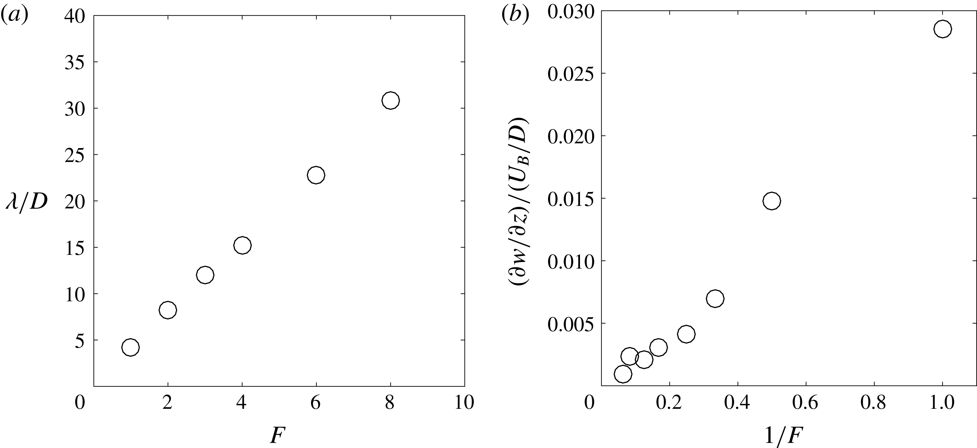
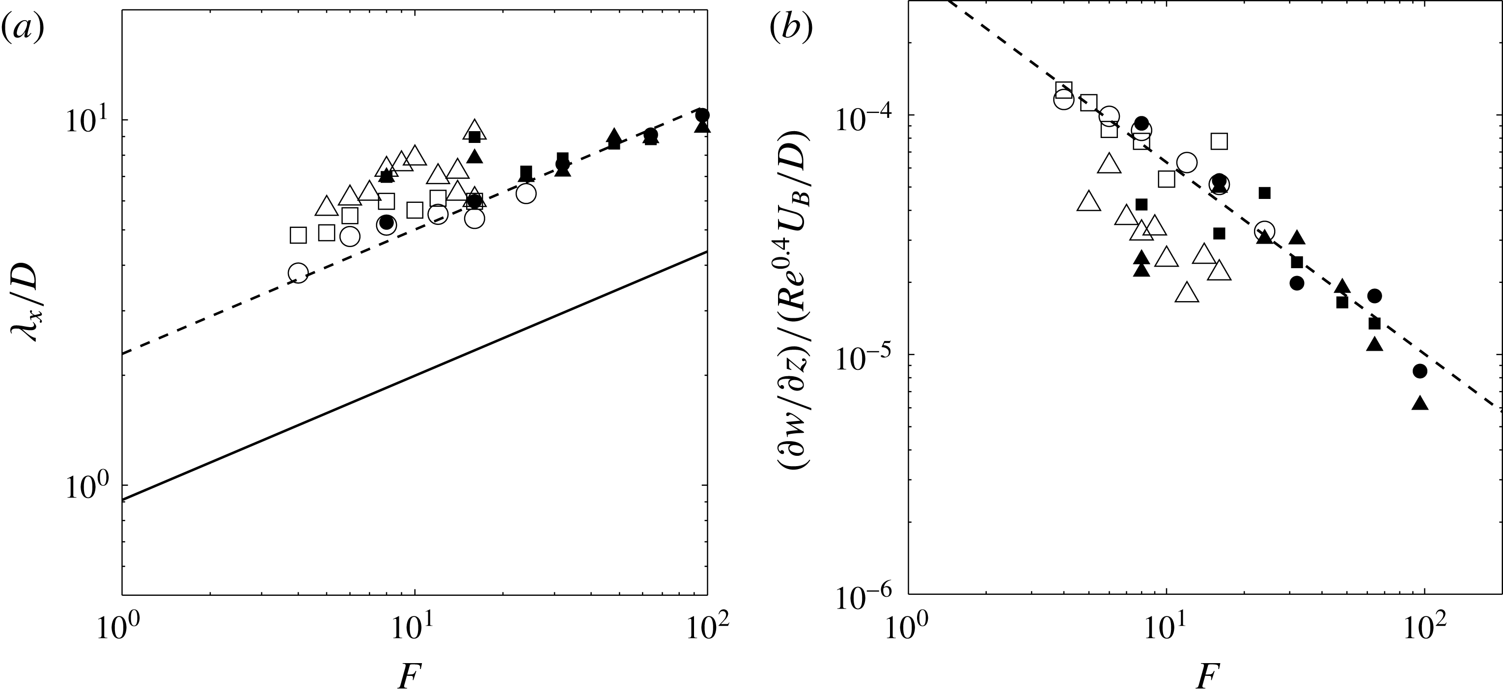
for two different Froude numbers. The wavelength is well defined on this type of profiles and clearly increases with the Froude number. For each Froude number, the wavelength has been measured over five wavelengths; it is plotted in figure 6(a) as a function of the Froude number. The wavelength increases linearly with the Froude number. This can be intuitively understood by the fact that a fluid particle oscillates at the frequency
 $N/(2\unicode[STIX]{x03C0})$
and is advected at the velocity
 $U_{B}$
. The wavelength is thus
 $\unicode[STIX]{x1D706}=2\unicode[STIX]{x03C0}U_{B}/N$
which can be rewritten
 $\unicode[STIX]{x1D706}/D=\unicode[STIX]{x03C0}F$
, in excellent quantitative agreement with the experimental measurements.
Mean vertical velocity gradient
 $\unicode[STIX]{x2202}w/\unicode[STIX]{x2202}z$
as a function of the downstream distance
 $x$
measured at
 $z=2D$
and
 $y=-3D$
for
 $F=1$
,
 $Re=600$
(solid line) and for
 $F=4$
,
 $Re=2400$
(dotted line).
 $z/H=0.629$
and
 $z_{0}/H=0.435$
.

(a) Wavelength of the lee waves measured at
 $z=2D$
and
 $y=-3D$
over the first five wavelengths. (b) Amplitude of the mean divergence at the first minimum located at
 $X=6FD\pm 10\,\%$
,
 $y=-3D$
and
 $z=2D$
. The Reynolds number is equal to
 $Re=600F$
.
 $h=H/D=10.2$
,
 $z/H=0.629$
and
 $z_{0}/H=0.435$
.

Figure 6(b) plots the amplitude of the lee waves. The maximum divergence is not measured at the first maximum which is too close to the sphere and is thus very noisy. This amplitude is rather measured at the first minimum of the
 $X$
-profiles, and is usually very close to the largest amplitude. This minimum is obtained close to
 $X/D=6F$
for all Froude numbers, which indicates that not only the wavelength but also the phase is proportional to the Froude number.
Figure 6(b) shows that the amplitude varies linearly with the inverse of the Froude number for
 $F\in [1,16]$
. Such a scaling seems similar to the scaling obtained by Bonneton et al. (Reference Bonneton, Chomaz and Hopfinger1993) for a Froude number ranging from 1 to 2. Indeed, they obtained that the displacement
 $\unicode[STIX]{x1D701}$
of the isopycnals is proportional to
 $F^{-1}$
. However, this would mean that the vertical velocity
 $w=\text{d}\unicode[STIX]{x1D701}/\text{d}t\sim (U_{B}/\unicode[STIX]{x1D706})\unicode[STIX]{x1D701}$
scales as
 $F^{-2}$
(since
 $\unicode[STIX]{x1D706}$
is proportional to
 $F$
) together with the vertical divergence. Our scaling of the vertical divergence as
 $F^{-1}$
is thus in disagreement with their measurements and their theoretical explanation. We will show in the following that their scaling is only valid at low Froude numbers and that an additional term must be taken into account at larger Froude numbers.
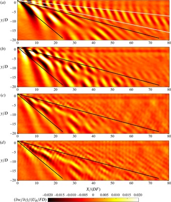
The various scalings of the amplitude and of the wavelength indicate that the lee waves seem to be self-similar such that
 $\unicode[STIX]{x2202}_{z}w$
must be dimensionalized by
 $U_{B}/(FD)$
and plotted as a function of
 $X/(FD)$
. This is what has been done in figure 7 for four different Froude numbers. The structure of the lee waves is now roughly independent of the Froude numbers. Most of the lee waves are emitted between the two black lines which correspond to angles equal to
 $15^{\circ }$
and
 $40^{\circ }$
for
 $F=1$
. However, at
 $F=1$
there is an additional structure of internal waves emitted at a smaller angle (located between the two white lines). We will show in the next theoretical section that this structure is a subcritical mode which can occur only at low Froude numbers. It also seems that the amplitude is slightly weaker for
 $F=8$
than for
 $F=1$
. It indicates that it decays slightly faster than
 $F^{-1}$
, especially for
 $F<2$
.
Mean vertical velocity gradient
 $\unicode[STIX]{x2202}w/\unicode[STIX]{x2202}z$
renormalized by the Froude number measured two diameters above the centre of the sphere at (a)
 $F=1$
,
 $Re=600$
, (b)
 $F=2$
,
 $Re=1200$
, (c)
 $F=4$
,
 $Re=2400$
and (d)
 $F=8$
,
 $Re=4800$
.
 $z/H=0.629$
and
 $z_{0}/H=0.435$
.

3.2 Lighthill theory
The calculation is adapted from the classical Lighthill theory and only the key points are given here. The details of the calculation are given in appendix A. For low amplitude, the structure of the lee waves is governed by the linearized Navier–Stokes equations for the velocity
 $\boldsymbol{u}=(u,v,w)$
in the Boussinesq approximation, together with the density equation and the incompressibility:
 $$\begin{eqnarray}\displaystyle & \displaystyle \displaystyle \frac{\unicode[STIX]{x2202}\boldsymbol{u}}{\unicode[STIX]{x2202}t}=\frac{-\unicode[STIX]{x1D735}p}{\unicode[STIX]{x1D70C}_{0}}-\frac{g\unicode[STIX]{x1D70C}}{\unicode[STIX]{x1D70C}_{0}}\boldsymbol{e}_{z}+{\mathcal{F}} & \displaystyle\end{eqnarray}$$
 $$\begin{eqnarray}\displaystyle & \displaystyle \displaystyle \frac{\unicode[STIX]{x2202}(g\unicode[STIX]{x1D70C}/\unicode[STIX]{x1D70C}_{0})}{\unicode[STIX]{x2202}t}-N^{2}w=0 & \displaystyle\end{eqnarray}$$
 $$\begin{eqnarray}\displaystyle & \displaystyle \unicode[STIX]{x1D735}\boldsymbol{\cdot }\boldsymbol{u}={\mathcal{Q}}. & \displaystyle\end{eqnarray}$$
 ${\mathcal{Q}}$
and
 ${\mathcal{F}}$
are two forcing terms stationary in the frame moving at the bluff body velocity.
 ${\mathcal{Q}}$
is the volumetric forcing term created by the moving boundaries of the bluff body. It is taken as a dipole in
 $x$
with a strength taken such that the induced velocity is equal to
 $-U_{B}$
at the surface of the sphere:
 $$\begin{eqnarray}{\mathcal{Q}}(x+U_{B}t,y,z)=(D/2)^{3}U_{B}\unicode[STIX]{x1D6FF}^{\prime }(x+U_{B}t)\unicode[STIX]{x1D6FF}(y)\unicode[STIX]{x1D6FF}(z-z_{0}),\end{eqnarray}$$
where
 $z_{0}$
is the vertical position of the sphere.
 ${\mathcal{F}}$
corresponds to the force exerted by the sphere on the fluid, which has been often neglected in previous studies. We have assumed that the force term has only an
 $x$
component
 ${\mathcal{F}}_{x}$
(no lift term). It is taken as a point force of strength given by the drag coefficient:
 $$\begin{eqnarray}{\mathcal{F}}_{x}={\textstyle \frac{1}{2}}C_{D}\unicode[STIX]{x03C0}(D/2)^{2}U_{B}^{2}\unicode[STIX]{x1D6FF}(x+U_{B}t)\unicode[STIX]{x1D6FF}(y)\unicode[STIX]{x1D6FF}(z-z_{0}).\end{eqnarray}$$
Manipulating these equations to eliminate variables leads to a forced internal wave equation for the vertical velocity component:
 $$\begin{eqnarray}\unicode[STIX]{x1D6FB}^{2}\displaystyle \frac{\unicode[STIX]{x2202}^{2}w}{\unicode[STIX]{x2202}t^{2}}+N^{2}\left(\displaystyle \frac{\unicode[STIX]{x2202}^{2}}{\unicode[STIX]{x2202}x^{2}}+\displaystyle \frac{\unicode[STIX]{x2202}^{2}}{\unicode[STIX]{x2202}y^{2}}\right)w=\displaystyle \frac{\unicode[STIX]{x2202}^{3}{\mathcal{Q}}}{\unicode[STIX]{x2202}z\unicode[STIX]{x2202}t^{2}}-\displaystyle \frac{\unicode[STIX]{x2202}^{3}{\mathcal{F}}_{x}}{\unicode[STIX]{x2202}x\unicode[STIX]{x2202}z\unicode[STIX]{x2202}t}.\end{eqnarray}$$
In the
 $z$
direction, the lee waves propagate rapidly such that they quickly fill the small height
 $H$
of fluid. The velocity is thus decomposed in a discrete sum of modes in the vertical direction. Since the buoyancy frequency is nearly constant in the experiment, the orthonormal modes are simply sine functions:
 $$\begin{eqnarray}w=\mathop{\sum }_{n=1}^{\infty }w_{n}(x+U_{B}t,y)\sqrt{\frac{2}{H}}\sin \left(\frac{n\unicode[STIX]{x03C0}z}{H}\right).\end{eqnarray}$$
Introducing this decomposition into (3.4) and taking the Fourier transform in
 $x$
and
 $y$
leads to an expression (see detailed calculation in appendix A) for the vertical velocity
 $$\begin{eqnarray}\frac{w}{U_{B}}=\mathop{\sum }_{n=1}^{\infty }n\unicode[STIX]{x03C0}\sin \left(\frac{n\unicode[STIX]{x03C0}z}{H}\right)\cos \left(\frac{n\unicode[STIX]{x03C0}z_{0}}{H}\right)\left[\frac{-D^{2}}{2\unicode[STIX]{x03C0}F^{2}H^{2}}I_{n}^{vol}(X,y)-\frac{C_{D}D^{2}}{4FH^{2}}I_{n}^{drag}(X,y)\right],\end{eqnarray}$$
where the volumetric mode is given by
 $$\begin{eqnarray}\!\!I_{n}^{vol}(X,y)=\int _{s_{n}}^{1}\frac{s^{2}\,\text{d}s}{\sqrt{1-s^{2}}\sqrt{\hat{n}^{2}-F^{-2}(1-s^{2})}}\cos \left(\frac{2sX}{DF}\right)\cos \left(\frac{2sy}{D}\sqrt{\frac{\hat{n}^{2}}{1-s^{2}}-F^{-2}}\right)\end{eqnarray}$$
and the drag mode is given by
 $$\begin{eqnarray}I_{n}^{drag}(X,y)=\int _{s_{n}}^{1}\frac{s\,\text{d}s}{\sqrt{1-s^{2}}\sqrt{\hat{n}^{2}-F^{-2}(1-s^{2})}}\sin \left(\frac{2sX}{DF}\right)\cos \left(\frac{2sy}{D}\sqrt{\frac{\hat{n}^{2}}{1-s^{2}}-F^{-2}}\right),\end{eqnarray}$$
with
 $\hat{n}=n\unicode[STIX]{x03C0}D/(2H)$
and
 $s_{n}=0$
for supercritical modes (defined by
 $\hat{n}F>1$
) and
 $s_{n}=(1-\hat{n}^{2}F^{2})^{1/2}$
for subcritical modes (defined by
 $\hat{n}F<1$
). It can be noted that the volumetric mode
 $I_{n}^{vol}(X,y)$
has a structure similar to the drag mode
 $I_{n}^{vol}(X,y)$
but in phase quadrature (see figure 22 in appendix A). The vertical velocity gradient
 $\unicode[STIX]{x2202}w/\unicode[STIX]{x2202}z$
is obtained from this formula by replacing
 $\sin (n\unicode[STIX]{x03C0}z/H)$
by
 $n\unicode[STIX]{x03C0}\cos (n\unicode[STIX]{x03C0}z/H)/H$
. In the volume and drag modes, the integrals are difficult to calculate since they strongly oscillate at large
 $X$
and
 $y$
. They can be approximated using the stationary phase method as shown in appendix B. However, this approximation fails at the cusps such that the full solution is used in the core of the paper. Numerically, the integrals were evaluated using the standard integration function ‘quad’ of Matlab which uses a recursive adaptive Simpson quadrature method. The tolerance was set to
 $10^{-7}$
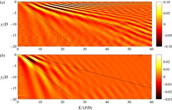
. The inviscid solution for
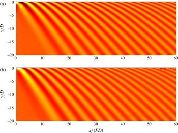
 $\unicode[STIX]{x2202}w/\unicode[STIX]{x2202}z$
is plotted in figure 8(a) for
 $F=4$
with a drag coefficient given by Blevins (Reference Blevins1984) as
 $C_{D}=0.4$
for the sphere in a homogeneous fluid for Reynolds numbers between
 $10^{3}$
and
 $10^{5}$
. The drag coefficient is only weakly affected by the stratification for
 $F>2$
. This solution presents dislocations (near
 $y/D=-3$
for
 $X/(FD)$
between 10 and 30) as in the experiments, which are due to interference between the discrete modes.
Theoretical prediction of the vertical velocity derivative
 $\unicode[STIX]{x2202}w/\unicode[STIX]{x2202}z/(U_{B}/FD)$
at (a)
 $Re=+\infty$
and (b)
 $Re=2400$
for a sphere with
 $F=4$
,
 $h=H/D=10.2$
.
 $z/H=0.629$
and
 $z_{0}/H=0.435$
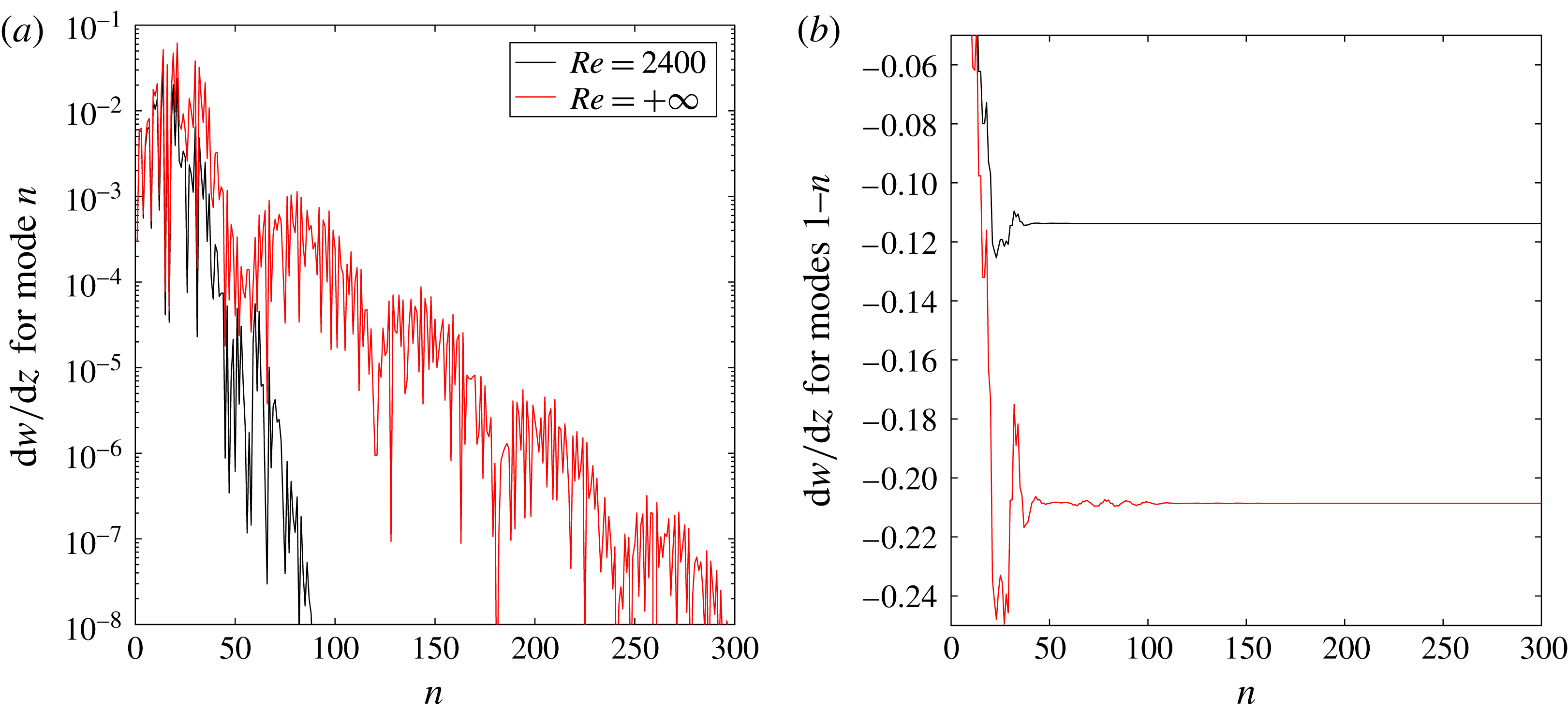
. Black lines correspond to 15 and 40 degree angles which surround most of the lee waves measured experimentally (plotted in figure 7). Thirty modes have been used in order to decreases the error down to 20 % in the viscous case. Robey (Reference Robey1997) only observed 2–3 modes since he used a larger sphere with a diameter of the order of the pycnocline thickness, leading to strong finite size effects (see § C.1).

However, it is clear that this solution is very different from the experimental result of figure 7(c). Indeed, the theoretical lee waves extend very far downstream close to the
 $X$
axis (up to
 $X/(FD)=60$
) whereas they quickly decay close to the
 $X$
axis in the PIV measurements. This is due to the presence of high modes in the theory (i.e. with high vertical wavenumber
 $n\unicode[STIX]{x03C0}/H$
). In the experiment, these modes are viscously damped and the theory must be modified in order to add viscous effects as shown by Scase & Dalziel (Reference Scase and Dalziel2006).
This is done by multiplying the amplitude of the wave by a decay factor
 $\exp (-\unicode[STIX]{x1D708}k^{2}t)$
where
 $k$
is the norm of the wavevector and
 $t=X/U_{B}$
. This term can be calculated as
 $\exp (-\unicode[STIX]{x1D708}Xn^{2}\unicode[STIX]{x03C0}^{2}/(U_{B}H^{2}(1-s)^{2}))$
and must be multiplied to the integrand of (3.7) and (3.8). This leads to a very different theoretical solution, as shown in figure 8(b) for the same Reynolds number as in the experiment
 $Re=2400$
. The internal waves are strongly damped close to the
 $X$
-axis for
 $X/FD$
larger than 20. The structure is now closer to the structure found experimentally. It should be noted that all experiments have been done with the bluff body towed close to mid-height (
 $z_{0}/H\sim 1/2$
). As seen in (3.6), the amplitude of odd modes is close to zero since
 $w$
is proportional to
 $\cos (n\unicode[STIX]{x03C0}z_{0}/H)$
. The amplitude of these modes is thus highly sensitive to the position of the bluff body, to the exact profile of stratification and to other additional effects. Several perturbative effects have been added to the theory (non-Boussinesq effects, surface waves at the free surface and finite size of the sphere) in order to explain this discrepancy (see appendix C). But their influence on the lee waves is negligible. It is possible that the experimental attenuation of the lee waves comes from a loss of coherence far from the wake axis due to the turbulent motions of the wake or to the nonlinearity of the density profile at the bottom and at the free surface.
For a quantitative comparison, the
 $x$
-wavelength of the lee waves has been measured theoretically on the first five lobes at
 $y/D=-3$
as in the experiment. The wavelength is proportional to the Froude number as in the experiment. It is equal to
 $$\begin{eqnarray}\unicode[STIX]{x1D706}=5.6F,\end{eqnarray}$$
within 0.3 %, which slightly overestimates the experimental values by 30 %. Furthermore, the amplitude of the lee waves has been measured as the minimum (over
 $X$
) of
 $\unicode[STIX]{x2202}w/\unicode[STIX]{x2202}z$
at
 $y/D=-3$
. This minimum is obtained close to
 $X/(FD)=7$
, which is close to the experimental position of the minimum (
 $X/(FD)=6$
).
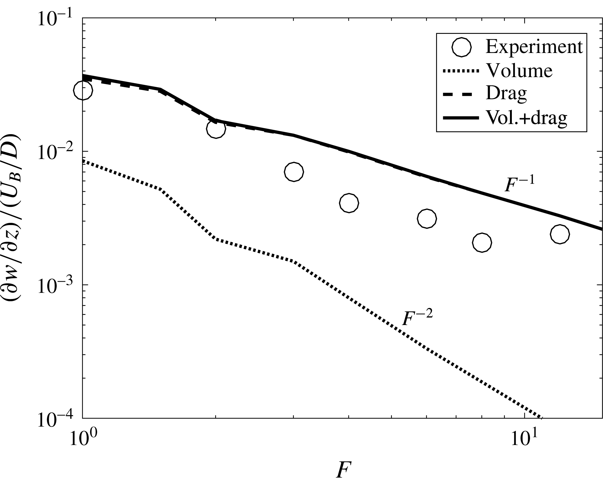
The amplitude is plotted in figure 9 as a function of the Froude number. The amplitude is first calculated for the volume source term
 ${\mathcal{Q}}$
only, then for the drag term
 ${\mathcal{F}}_{x}$
only and finally for both source terms. It is clear from this figure that the volume source term is negligible compared to the drag term at moderate and large Froude numbers (for
 $F>2$
). This can be explained by the fact that in (3.6) the volume mode
 $I_{n}^{vol}$
is divided by
 $F^{2}$
whereas the drag mode
 $I_{n}^{drag}$
is divided by
 $F$
. As a consequence, the amplitude of the drag (respectively volume) term scales as
 $F^{-1}$
(respectively
 $F^{-2}$
) in figure 9. The total amplitude thus scales as
 $F^{-1}$
for
 $F>2$
, in excellent quantitative agreement with the experimental result. For Froude numbers smaller than 1, the volume term may become dominant, leading to a different scaling. This can explain the scaling measured by Bonneton et al. (Reference Bonneton, Chomaz and Hopfinger1993) for
 $1<F<2$
, which can be translated into
 $\unicode[STIX]{x2202}w/\unicode[STIX]{x2202}z\sim F^{-2}$
. For larger Froude numbers, Robey (Reference Robey1997) had noted that the amplitude was smaller in the model than in the experiments. He fixed the problem by taking into account the recirculation bubble (of finite downstream size) behind the bluff body. This translated the maximum of the amplitude toward larger Froude numbers but did not modify the scaling. Here, we have considered the drag which creates a recirculating jet (of infinite downstream size) behind the bluff body, leading to the separation of the flow. This extension of Robey’s ideas gives a better agreement on a larger range of Froude numbers.
Amplitude of the vertical velocity derivative
 $\unicode[STIX]{x2202}w/\unicode[STIX]{x2202}z$
at
 $y/D=-3$
and
 $z/D=2$
. The theory is obtained for the volume source term only (dotted line), for the drag source term only (dashed line) and for both source terms (solid line).
 $Re=600F$
,
 $h=H/D=10.2$
,
 $z/H=0.629$
and
 $z_{0}/H=0.435$
.

It is very interesting to see that the drag term is in fact the dominant term at moderate and large Froude numbers. Indeed, most of the theoretical studies have been done by considering the volume source term only. This simple and poorly known contribution should probably be taken into account in most geophysical stratified wakes.
3.3 Influence of the shape of the bluff body
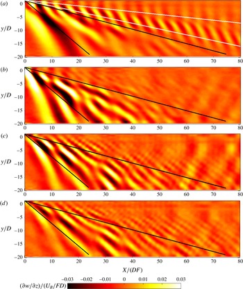
Experiments using two different bluff bodies have been done in order to quantify the influence of the shape of the bluff body. First, a 6 : 1 cylinder has been translated horizontally along its axis. The rescaled divergence has been measured by PIV and averaged in the frame of reference of the bluff body as done with the sphere. This quantity (which reveals the lee waves) is plotted in figure 10 for 4 different Froude numbers. As for the sphere, the lee waves contain a subcritical mode for
 $F=1$
only, which propagates at an angle between
 $6^{\circ }$
and
 $12^{\circ }$
(plotted as white lines). The lee waves also contain supercritical modes for all Froude numbers, which propagate at an angle between
 $15^{\circ }$
and
 $40^{\circ }$
(plotted as black lines) exactly as for the sphere. The isophases exhibit dislocations which reveal the interference of several supercritical modes.
Mean vertical velocity gradient
 $\unicode[STIX]{x2202}w/\unicode[STIX]{x2202}z$
renormalized by the Froude number measured two diameters above the centre of the 6 : 1 cylinder at (a)
 $F=1$
,
 $Re=740$
, (b)
 $F=2$
,
 $Re=1480$
, (c)
 $F=4$
,
 $Re=2960$
and (d)
 $F=8$
,
 $Re=5920$
.
 $z/H=0.606$
and
 $z_{0}/H=0.403$
.

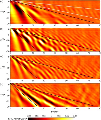
Second, a 6 : 1 spheroid has been translated along its major axis. The lee waves of the spheroid are shown in figure 11 for four different Froude numbers. They are exactly similar to the lee waves of the cylinder and the sphere. They exhibit a subcritical mode for
 $F=1$
only and several supercritical modes for all Froude numbers.
Mean vertical velocity gradient
 $\unicode[STIX]{x2202}w/\unicode[STIX]{x2202}z$
renormalized by the Froude number measured two diameters above the centre of the 6 : 1 spheroid at (a)
 $F=1$
,
 $Re=680$
, (b)
 $F=2$
,
 $Re=1360$
, (c)
 $F=4$
,
 $Re=2720$
and (d)
 $F=8$
,
 $Re=5440$
.
 $z/H=0.596$
and
 $z_{0}/H=0.401$
.

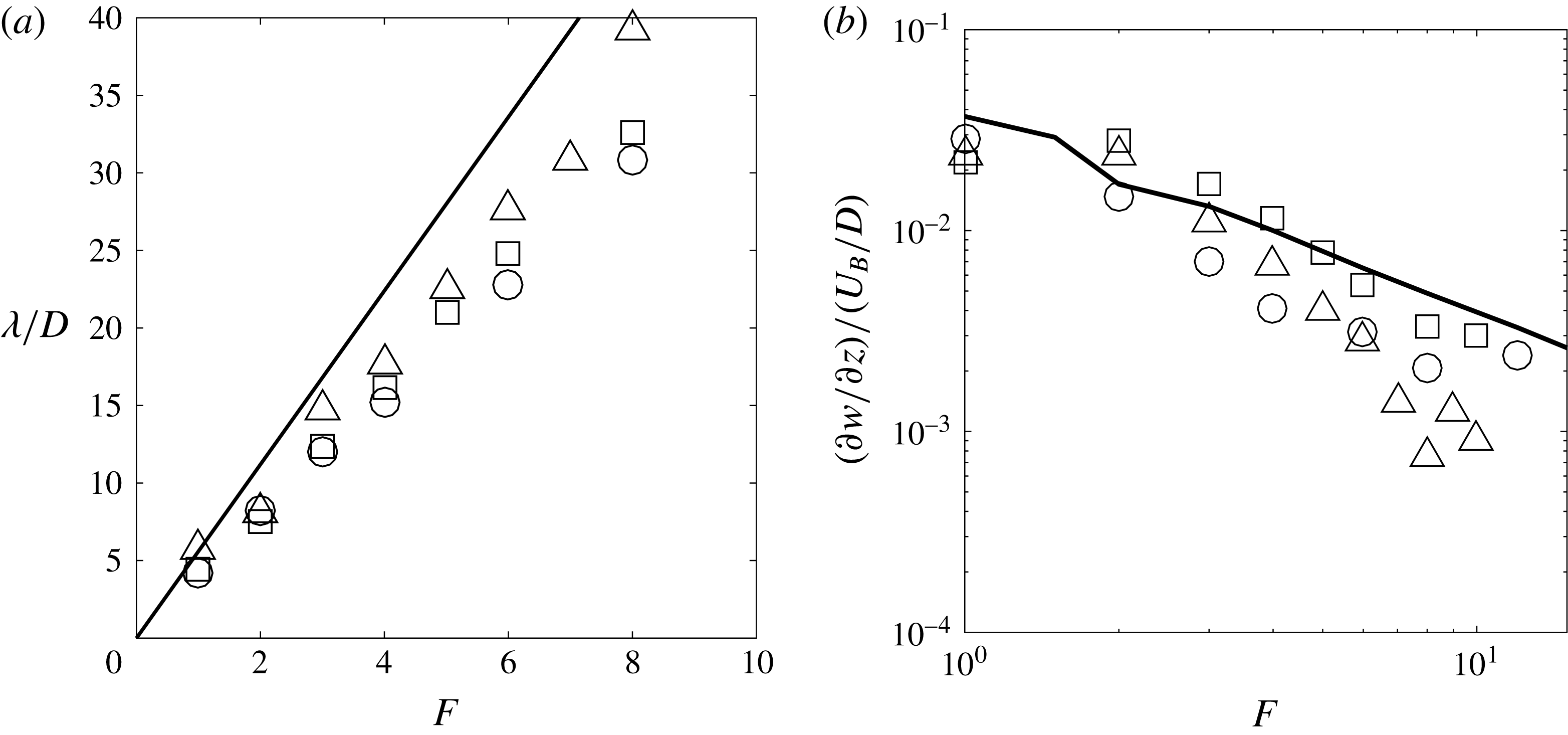
The wavelength of the lee waves have been measured for the cylinder and the spheroid. They are plotted in figure 12(a) and show a linear variation with the Froude number for
 $1<F<8$
. They are slightly larger than the wavelength of the sphere (by approximately 5 % for the cylinder and by approximately 15 % for the spheroid). The model obtained from the Lighthill theory (plotted as a solid line in figure 12
a) is in fair agreement with these experimental measurements although overpredicting the wavelength by 20 %.
(a) Wavelength of the lee waves measured at
 $z=2D$
and
 $y=-3D$
over the first five wavelengths. (b) Amplitude of the mean divergence at the first minimum located at
 $x=6FD\pm 20\,\%$
,
 $y=-3D$
and
 $z=2D$
. Symbols correspond the experimental measurements for a sphere (○), a 6 : 1 cylinder (▫) and a 6 : 1 spheroid (▵). Solid lines correspond to the theory for a sphere with the volumetric and the drag terms. The Reynolds number is approximately equal to
 $Re=600F$
.

The amplitude
 $\unicode[STIX]{x2202}w/\unicode[STIX]{x2202}z$
has also been measured at the first minimum of the
 $x$
-profiles at
 $y=-3D$
. For the 6 : 1 cylinder, the amplitude seems to scale as
 $F^{-1}$
as for the sphere. This indicates that the lee waves are created by the drag term rather than the volumetric term. Moreover, the amplitude is approximately twice as large for the cylinder as for the sphere. This is consistent with the fact that the drag coefficient is approximately twice as large for a cylinder as for a sphere. It thus seems that the Lighthill theory developed in the last subsection successfully predicts the amplitude of the lee waves of a cylinder since the drag term in (3.6) is proportional to the drag coefficient. For the spheroid, the amplitude is smaller than the amplitude of the sphere for
 $F>5$
. This is consistent with the fact that the drag coefficient is approximately twice smaller for a spheroid than for a sphere. However, for
 $F<5$
, the amplitude is larger for the spheroid than for the sphere. This could be explained by the fact that the volumetric term (which becomes dominant at small Froude numbers) may be larger for the spheroid than for the sphere. As a consequence, it seems that the amplitude of the lee waves scale as
 $F^{-2}$
for the spheroid.
4 Wake waves
As noted at the end of § 2, the wake waves propagate in the
 $x$
-direction slower than the lee waves which propagate at the bluff body velocity
 $U_{B}$
. In the previous section, this property was used to filter out the wake waves by averaging the velocity fields in the frame moving at
 $U_{B}$
. In this section, the lee waves will be filtered out by averaging the fields in a frame moving at the phase velocity
 $U_{\unicode[STIX]{x1D719}}$
of the wake waves. This procedure also helps to filter out the disturbances created by the turbulent motions within the wake itself (i.e. close to the centreline).
4.1 Phase velocity of the wake waves
To do so, the phase velocities
 $U_{\unicode[STIX]{x1D719}}$
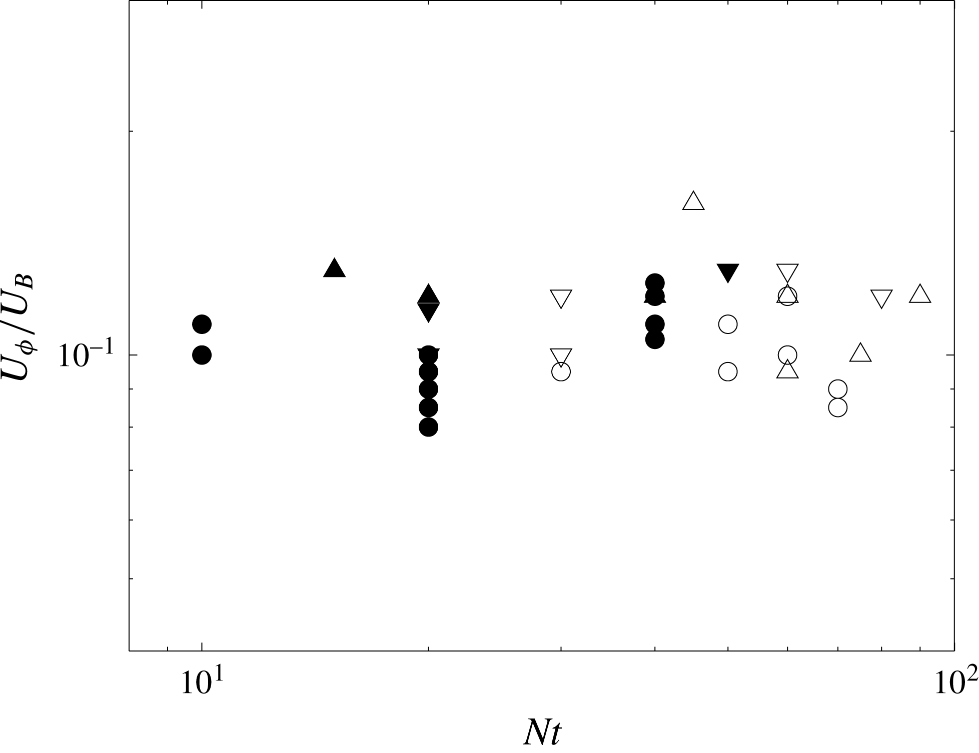
of the wake waves need to be determined accurately. They have been measured on spatio-temporal diagrams similar to the one in figure 3. They are reported in figure 13 for
 $F=8$
, where each symbol corresponds to a line identified in the spatio-temporal diagram. The phase velocity
 $U_{\unicode[STIX]{x1D719}}$
corresponds to the inverse of the slope and the time is taken at the middle of the line. Figure 13 indicates that the phase velocity is nearly constant in time although the waves are measured on a large period (between
 $Nt=10$
and
 $Nt=100$
). Moreover, the phase velocity is independent of the location at which it is measured (in
 $y$
and in
 $z$
) and also independent of the Reynolds number.
Phase velocity of the wake waves as a function of time measured at
 $z=1D$
(circles) and at
 $z=2D$
(triangles). Filled symbols are obtained at
 $y=1.5D$
and open symbols at
 $y=5D$
.
 $F=8$
,
 $Re=4850$
(except for ▿:
 $Re=1260$
).

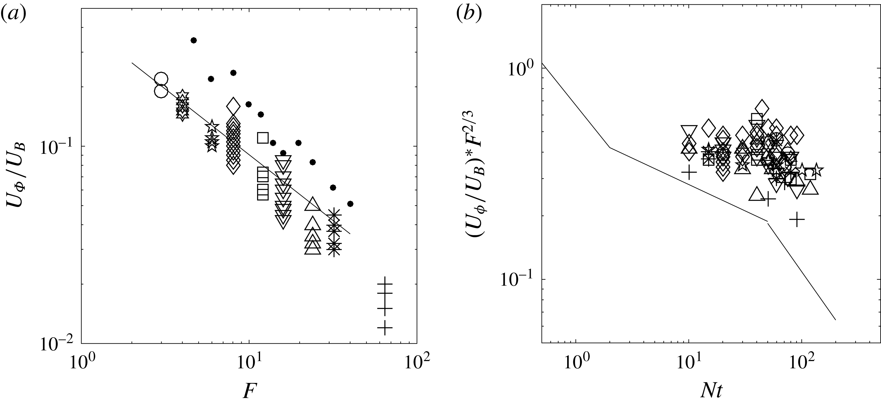
Phase velocity of the wake waves (a) as a function of the Froude number and (b) as a function of time rescaled by
 $F^{2/3}$
. Dotted symbols correspond to the experimental results of Robey (Reference Robey1997). The solid line corresponds to the wake velocity defect given by Spedding (Reference Spedding1997), taken from (4.1) at
 $Nt=2$
in (a). Symbols in (b) correspond to the same Froude numbers as in (a).
 $z=2D$
.

However, the phase velocity
 $U_{\unicode[STIX]{x1D719}}$
strongly depends on the Froude number, as shown in figure 14(a). These experimental measurements are compared to the phase velocities measured by Robey (Reference Robey1997) (small black round symbols) which are larger by up to a factor 2. This is probably because the results of Robey (Reference Robey1997) are obtained for a thin thermocline (approximately ten times smaller than the sphere) whereas our results are obtained for a thick thermocline (about ten times larger than the sphere). The phase velocity scales as
 $F^{-2/3}$
and corresponds exactly to the velocity defect of the wake at
 $Nt=2$
(shown as a solid line in figure 14
a) and given by Spedding (Reference Spedding1997) as
 $$\begin{eqnarray}\frac{U}{U_{B}}=0.5(Nt)^{-0.25}\quad \text{for }1.7<Nt<50.\end{eqnarray}$$
As already explained by Robey (Reference Robey1997), this indicates that the waves are probably emitted by the coherent structures (pancake vortices) which move at the wake velocity. For
 $Nt\ll 2$
, the local Froude number of the vortices is larger than 1 such that the waves emitted have a very small amplitude. At
 $Nt=2$
, the local Froude number is equal to 1 such that the amplitude of the emitted waves is maximum. This creates a burst of internal waves which propagate slowly in the vertical direction for
 $Nt>2$
. These waves are then observed between
 $Nt=10$
and
 $Nt=100$
when they reach the measurement plane (see figure 14). As time increases, the velocity defect decreases such that the amplitude of the emitted waves decreases. This probably creates slower and less energetic waves that may be observed later. This effect could explain the weak decay (by approximately 30 %) observed in figure 14(b) between the early waves (
 $Nt=10$
) and the late waves (
 $Nt=100$
). This effect is clearly visible in the simulations of Zhou & Diamessis (Reference Zhou and Diamessis2016) since the measurement plane is farther (
 $z/D=9$
). It should be noted that there are large fluctuations (of the order of 50 %) of the phase velocity in a single experiment. These fluctuations are much larger than the noise in the measurement (of the order of 10 %) and reflect the strong fluctuations of the turbulent wake itself.
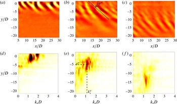
Velocity divergence (a–c) and corresponding
 $x$
-spectra (d–f) of the wake waves. The fields are obtained at
 $Nt=16.3$
(a,d), 60 (b,e), 130 (c,f), averaged over six velocity fields, i.e.
 $N\unicode[STIX]{x0394}t=16$
.
 $F=8$
,
 $Re=4850$
,
 $z=2D$
.

4.2 Divergence fields
This accurate characterization of the phase velocity is now used to average the velocity fields in the frame of reference moving with the wake waves at
 $U_{\unicode[STIX]{x1D719}}$
. An example of the divergence
 $\unicode[STIX]{x2202}w/\unicode[STIX]{x2202}z$
is plotted in figure 15(a–c) averaged over an optimized duration (
 $\unicode[STIX]{x0394}t=8.5~\text{sec}$
). At
 $Nt=16$
, the wake waves are clearly visible with isophases oriented at
 $50^{\circ }$
with respect to the
 $x$
-axis. At early times, the waves are located directly above the sphere wake (around
 $y=0$
). At later times, the waves propagate away from the wake centreline, creating two bands filled with internal waves on each side of the centreline (for
 $2<|y|/D<8$
at
 $Nt=60$
). At very late stages, some waves are visible very far from the centreline (for
 $6<|y|/D<18$
at
 $Nt=130$
). However, a dislocation at
 $|y|/D=10$
tends to indicate that the waves at
 $|y|/D>10$
are due to a reflection of the waves at the free surface.
These internal waves are similar to the wake waves obtained numerically by Abdilghanie & Diamessis (Reference Abdilghanie and Diamessis2013) and observed experimentally by Robey (Reference Robey1997). They also bear some similarities with the ‘random waves’ observed by Bonneton et al. (Reference Bonneton, Chomaz and Hopfinger1993). However, the ‘semi-circular concentric waves’ observed at a smaller wavelength by Bonneton et al. (Reference Bonneton, Chomaz and Hopfinger1993) are not visible here.
The velocity divergence fields have been Fourier transformed in
 $x$
in order to measure the
 $x$
-wavelength. At each cross-stream position
 $y$
, the
 $x$
-Fourier transforms are calculated and then plotted as a stack in figure 15(d–f). The spectra exhibit a peak which propagates towards large
 $y$
while remaining at a fixed wavenumber (
 $K_{x}/D\approx 1.2$
). The peak is relatively broad (
 $1<K_{x}D<2$
) probably due to the irregularity of the von Kármán wake.
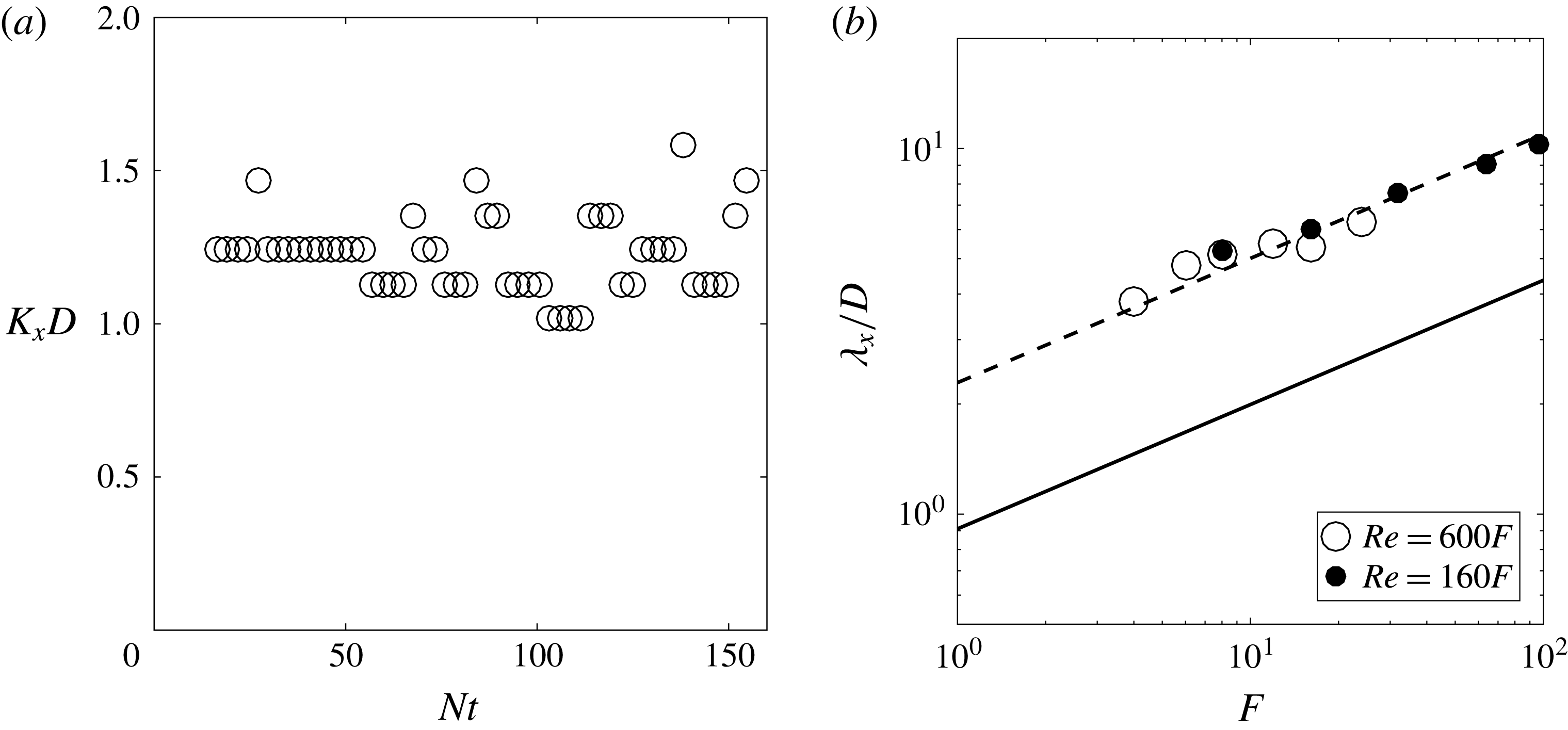
(a) Temporal evolution of the maximum streamwise wavenumber. (b) Wavelength of the wake waves as a function of the Froude number. Lines correspond to the wavelength of the von Kármán vortex street (i.e. the distance between same sign vortices) given by (4.2) at
 $Nt=2$
(solid line) and at
 $Nt=30$
(dotted line).
 $z=2D$
.

4.3 Characteristics of the wake waves
The
 $x$
-wavenumber
 $K_{x}$
corresponding to this peak is plotted in figure 16(a) as a function of time. It is nearly constant up to
 $Nt=160$
and can be extracted for each run. This wavenumber is not modified when the measurement plane is located one diameter above the sphere. The corresponding
 $x$
-wavelength
 $\unicode[STIX]{x1D706}_{x}^{w}=2\unicode[STIX]{x03C0}/K_{x}$
is plotted in figure 16(b) as a function of the Froude number. It scales as
 $F^{1/3}$
which is similar to the wake horizontal width and to the distance between same sign vortices. This is coherent with a burst of internal waves emitted by the von Kármán vortex street whose wavelength sets the wavelength of the emitted waves. The distance between same sign vortices has been found experimentally by Spedding (Reference Spedding2002) to be equal to
 $$\begin{eqnarray}\frac{\unicode[STIX]{x1D706}_{x}}{D}=0.71(Nt)^{0.34}F^{0.34}.\end{eqnarray}$$
This prediction is plotted as a solid line in figure 16(b) assuming that the waves are emitted at the beginning of the NEQ regime (i.e. for
 $Nt=2$
). Unfortunately, this prediction is twice smaller than the experimental results. An excellent agreement is obtained by assuming that the internal waves are emitted by the von Kármán vortices at
 $Nt=30$
(plotted as a dotted line) rather than at
 $Nt=2$
. However, this is in disagreement with the phase velocity of the waves measured previously which indicated that the waves are emitted at
 $Nt=2$
. It should be noted that the wavelength depends very weakly on the Reynolds number: it decreases by only 10 % when the Reynolds number increases by a factor 4. This is slightly smaller than the Reynolds dependence obtained by Zhou & Diamessis (Reference Zhou and Diamessis2016) far above the wake. This suggests that it could be due to an attenuation of the small wavelengths during their propagation. However, it should be noted that this
 $x$
-wavenumber does not correspond to the horizontal wavenumber
 $k_{H}$
measured by Abdilghanie & Diamessis (Reference Abdilghanie and Diamessis2013) and Zhou & Diamessis (Reference Zhou and Diamessis2016) which is a two-dimensional (2-D) wavenumber
 $k_{H}=\sqrt{k_{x}^{2}+k_{y}^{2}}$
.
The
 $y$
-location of the maximum of the spectrum has also been measured for each spectrum. This position
 $y^{w}$
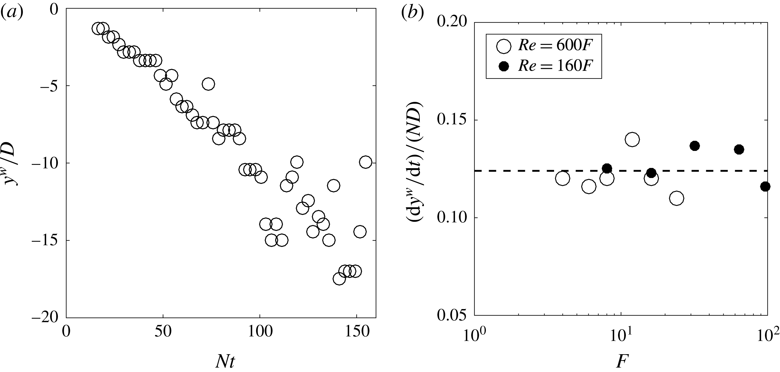
, which corresponds to the distance between the wake centreline and the band of internal waves, is plotted in figure 17(a) as a function of time. It increases linearly with time. This is consistent with a burst of internal waves emitted at early times, which propagates with a constant group velocity. The horizontal velocity of the wavepacket has been extracted for all Froude numbers. It seems to be well fitted by the dimensional law:
 $$\begin{eqnarray}\frac{\text{d}y^{w}}{\text{d}t}=0.125ND.\end{eqnarray}$$
This velocity is smaller by a factor 2 to 6 to the streamwise velocity of the waves
 $U_{\unicode[STIX]{x1D719}}$
. Moreover, it does not have the same scaling than
 $U_{\unicode[STIX]{x1D719}}$
which scales as
 $F^{1/3}ND$
. It should be noted that the position
 $y^{w}$
is identical at
 $z=D$
and
 $z=2D$
.
Cross-stream position
 $y_{w}$
(a) and cross-stream velocity
 $\text{d}y_{w}/\text{d}t$
(b) of the maximum of the wake waves. In (a),
 $F=8$
,
 $Re=4850$
.
 $z=2D$
.

The angle
 $\unicode[STIX]{x1D6FC}^{w}$
of the isophases with respect to the centreline (see schematic definition in figure 15
b) can be extracted by calculating the 2-D Fourier spectrum of each instantaneous divergence field (not shown here). The angle
 $\unicode[STIX]{x1D6FC}^{w}$
is simply given by
 $\tan (\unicode[STIX]{x1D6FC}^{w})=K_{x}/K_{y}$
where
 $(K_{x},K_{y})$
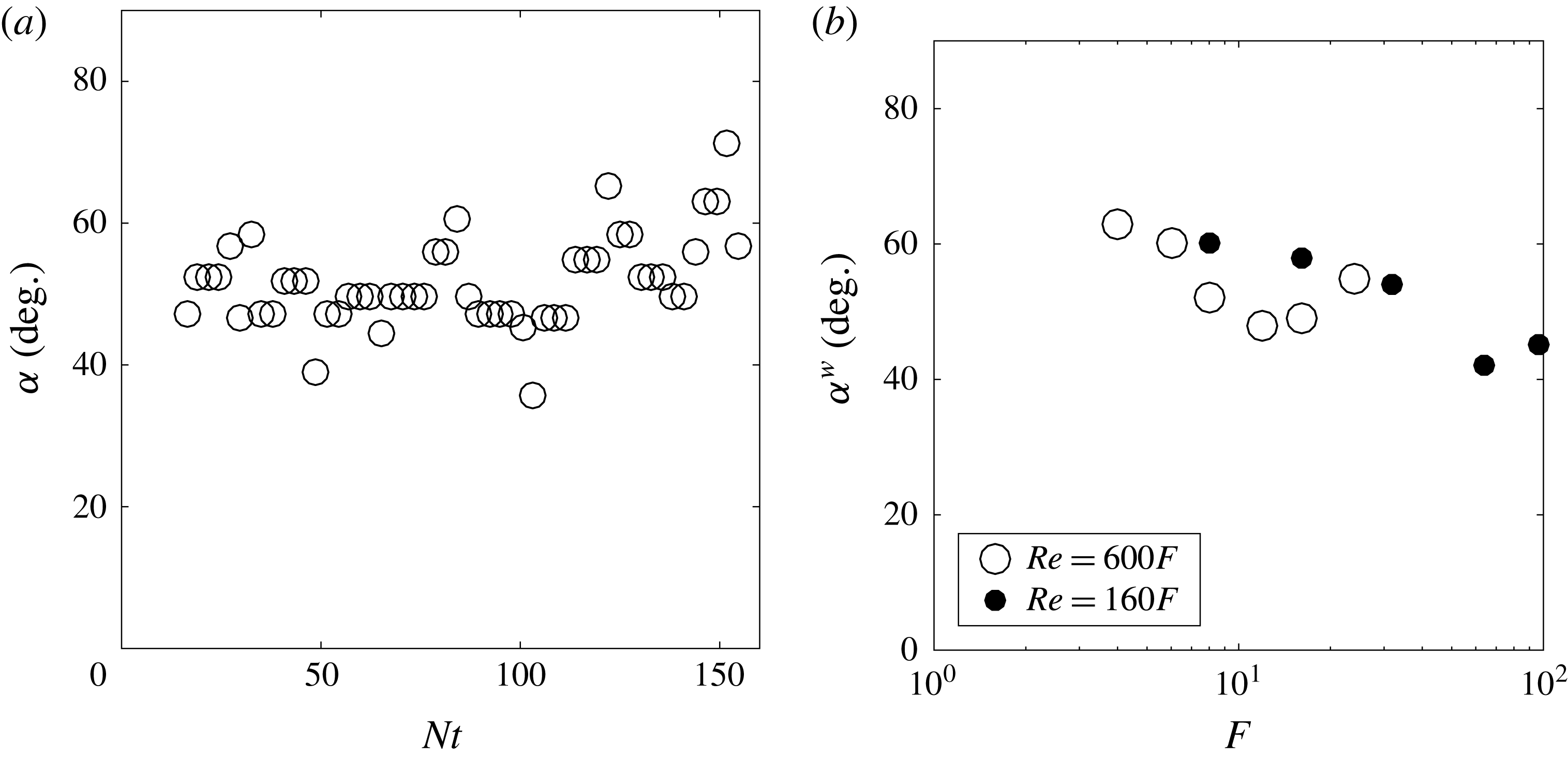
correspond to the position of the maximum of the 2-D spectrum. It is plotted as a function of time in figure 18(a) and seems to be roughly constant around
 $50^{\circ }$
. The small increase at late stages may not be relevant since it might be related to waves reflected at the free surface. The mean angle is then plotted as a function of the Froude number in figure 18(b). The angle
 $\unicode[STIX]{x1D6FC}^{w}$
decreases from
 $55^{\circ }$
to
 $45^{\circ }$
when the Froude number increases from
 $F=4$
to
 $F=96$
. It should be noted that this tilt angle is independent of the Reynolds number and remains unchanged between
 $z=D$
and
 $z=2D$
.
Angle of the horizontal wavevector (a) as a function of time and (b) as a function of
 $F$
. In (a),
 $F=8$
,
 $Re=4850$
.
 $z=2D$
.

4.4 Amplitude of the wake waves
Finally, the amplitude of the wake waves is measured as the root mean square (r.m.s.) value of the divergence of the wake waves on the line
 $y/D=-3$
. This amplitude strongly depends on time and is maximum around
 $Nt=25$
for any Froude and Reynolds number. This reflects the fact that the waves propagate horizontally at a velocity
 $\text{d}y^{w}/\text{d}t$
independent of
 $F$
and
 $Re$
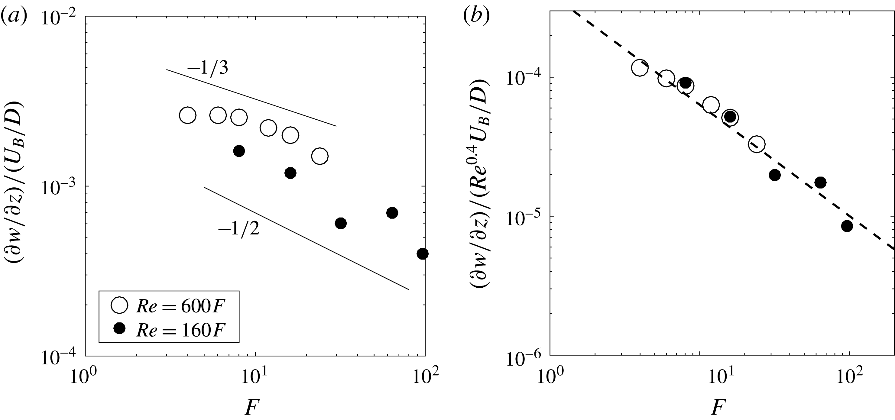
. The maximum amplitude is plotted in figure 19(a) as a function of the Froude number. The amplitude seems to decrease as
 $F^{\unicode[STIX]{x1D6FE}}$
with an exponent
 $\unicode[STIX]{x1D6FE}$
between
 $-1/2$
and
 $-1/3$
. Such a scaling is consistent with the results by Bonneton et al. (Reference Bonneton, Chomaz and Hopfinger1993) and Robey (Reference Robey1997) who found that the displacement
 $\unicode[STIX]{x1D701}$
of the isopycnal seems proportional to the Froude number. Indeed, the velocity divergence
 $\unicode[STIX]{x2202}w/\unicode[STIX]{x2202}z$
is equal to
 $\text{i}k_{z}w$
where the vertical velocity
 $w=\text{d}\unicode[STIX]{x1D701}/\text{d}t$
is the product of the frequency of the wave
 $\unicode[STIX]{x1D714}=ik_{x}U_{\unicode[STIX]{x1D719}}$
(similar to a Doppler shift) times the displacement
 $\unicode[STIX]{x1D701}$
. It leads to an expression for the velocity divergence:
 $$\begin{eqnarray}\frac{\unicode[STIX]{x2202}w}{\unicode[STIX]{x2202}z}=-k_{z}k_{x}U_{\unicode[STIX]{x1D719}}\unicode[STIX]{x1D701}.\end{eqnarray}$$
Assuming that the vertical wavenumber
 $k_{z}$
scales as the horizontal wavenumber
 $k_{x}\sim F^{-1/3}$
and taking into account the scaling
 $U_{\unicode[STIX]{x1D719}}\sim F^{-2/3}$
leads to a scaling for the velocity divergence as
 $$\begin{eqnarray}\frac{\unicode[STIX]{x2202}w/\unicode[STIX]{x2202}z}{U_{B}/D}\sim F^{-4/3}\frac{\unicode[STIX]{x1D701}}{D}.\end{eqnarray}$$
A scaling of the velocity divergence
 $\unicode[STIX]{x2202}w/\unicode[STIX]{x2202}z\sim F^{-1/3}$
is thus consistent with a scaling of the displacement
 $\unicode[STIX]{x1D701}\sim F$
observed by Robey (Reference Robey1997) and Bonneton et al. (Reference Bonneton, Chomaz and Hopfinger1993). Moreover, the quantitative value
 $\unicode[STIX]{x1D701}=0.005F$
given by Bonneton et al. (Reference Bonneton, Chomaz and Hopfinger1993) is in quantitative agreement with the divergence obtained in our experiments.
Maximum amplitude of the r.m.s. divergence as a function of the Froude number at
 $y/D=-3$
and
 $z/D=2$
. The dashed line corresponds to a fit of the experimental data scaling as
 $F^{-0.8}$
.

However, all these experiments are obtained with a varying Reynolds number which may drastically modify the scaling in Froude number at a fixed Reynolds number. Indeed, figure 19(a) indicates that the amplitude is approximately twice larger for the large Reynolds number experiments (
 $D=2.52~\text{cm}$
, large open symbols) than for the small Reynolds number experiments (
 $D=1.28~\text{cm}$
, small filled symbols). It means that the amplitude must be rescaled by
 $Re^{0.4}$
in order to collapse all data. Such a dependence on the Reynolds number has already been observed numerically by Abdilghanie & Diamessis (Reference Abdilghanie and Diamessis2013) although they obtained a weaker exponent for the wave momentum flux:
 $\langle uw\rangle \sim Re^{0.25}$
. The rescaled amplitude of the divergence is plotted in figure 19(b) and shows a reasonable collapse for the two series of Reynolds numbers. As a consequence, the scaling with the Froude number is modified and seems to be close to
 $F^{-0.8}$
. This scaling is close to the scaling of the velocity defect
 $U_{0}$
(and the phase velocity
 $U_{\unicode[STIX]{x1D719}}$
) as
 $F^{-2/3}$
. This Froude dependence is in excellent agreement with the results by Abdilghanie & Diamessis (Reference Abdilghanie and Diamessis2013) who found that the momentum flux
 $\langle uw\rangle$
decreases slightly faster with respect to
 $F$
than the squared velocity defect
 $U_{0}^{2}$
at a fixed Reynolds number.
The best fit of the amplitude gives:
 $$\begin{eqnarray}\frac{\unicode[STIX]{x2202}w/\unicode[STIX]{x2202}z}{U_{B}/D}=0.0004Re^{0.4}F^{-0.8}.\end{eqnarray}$$
So far, there is no explanation for the dependence of the amplitude with the Reynolds number. It is possible that the wake becomes more turbulent and irregular at larger Reynolds numbers leading to a more energetic emission of internal waves on a longer duration. Further experiments at larger Reynolds numbers might be necessary in order to confirm the validity of the scalings at large Reynolds numbers.
Finally, it should be mentioned that the amplitude of the wake waves is smaller than the lee waves by an order of magnitude when extrapolating these results to
 $F=1$
. However, the wake waves become dominant for Froude numbers larger than 10, in agreement with the results of Bonneton et al. (Reference Bonneton, Chomaz and Hopfinger1993).
4.5 A simple model
It is possible to calculate theoretically the internal waves emitted by a von Kármán vortex street. The vortices are supposed to be separated by a wavelength
 $\unicode[STIX]{x1D706}_{x}=2\unicode[STIX]{x03C0}/k_{x}$
between same sign vortices given by (4.2). The distance between the two rows of vortices is taken as
 $d=0.4\unicode[STIX]{x1D706}_{x}$
which is characteristic of stratified wakes (Meunier & Spedding Reference Meunier and Spedding2004). The vortices are supposed to move at the velocity
 $U_{\unicode[STIX]{x1D719}}$
given by (4.1). The low pressures at the centre of each vortex creates a perturbation which is periodic in
 $x$
for each row of vortices. The pressure perturbation is thus taken at
 $z=0$
as
 $$\begin{eqnarray}p(x,y,t)=\left[\unicode[STIX]{x1D6FF}\left(y-\frac{\text{d}}{2}\right)-\unicode[STIX]{x1D6FF}\left(y+\frac{\text{d}}{2}\right)\right]\cos [k_{x}(x+U_{\unicode[STIX]{x1D719}}t)].\end{eqnarray}$$
The internal waves emitted by this pressure perturbation are simply given for large
 $y$
and
 $z$
by
 $$\begin{eqnarray}p(X,y,z)=\text{Re}[\text{e}^{\text{i}k_{x}X}\text{e}^{\text{i}\sqrt{(N^{2}/U_{\unicode[STIX]{x1D719}}^{2}-k_{x}^{2})z^{2}-k_{x}^{2}(y-d/2)^{2}}}-\text{e}^{\text{i}k_{x}X}\text{e}^{\text{i}\sqrt{(N^{2}/U_{\unicode[STIX]{x1D719}}^{2}-k_{x}^{2})z^{2}-k_{x}^{2}(y+d/2)^{2}}}],\end{eqnarray}$$
where
 $\text{Re}$
is the real part and
 $X=x+U_{\unicode[STIX]{x1D719}}t$
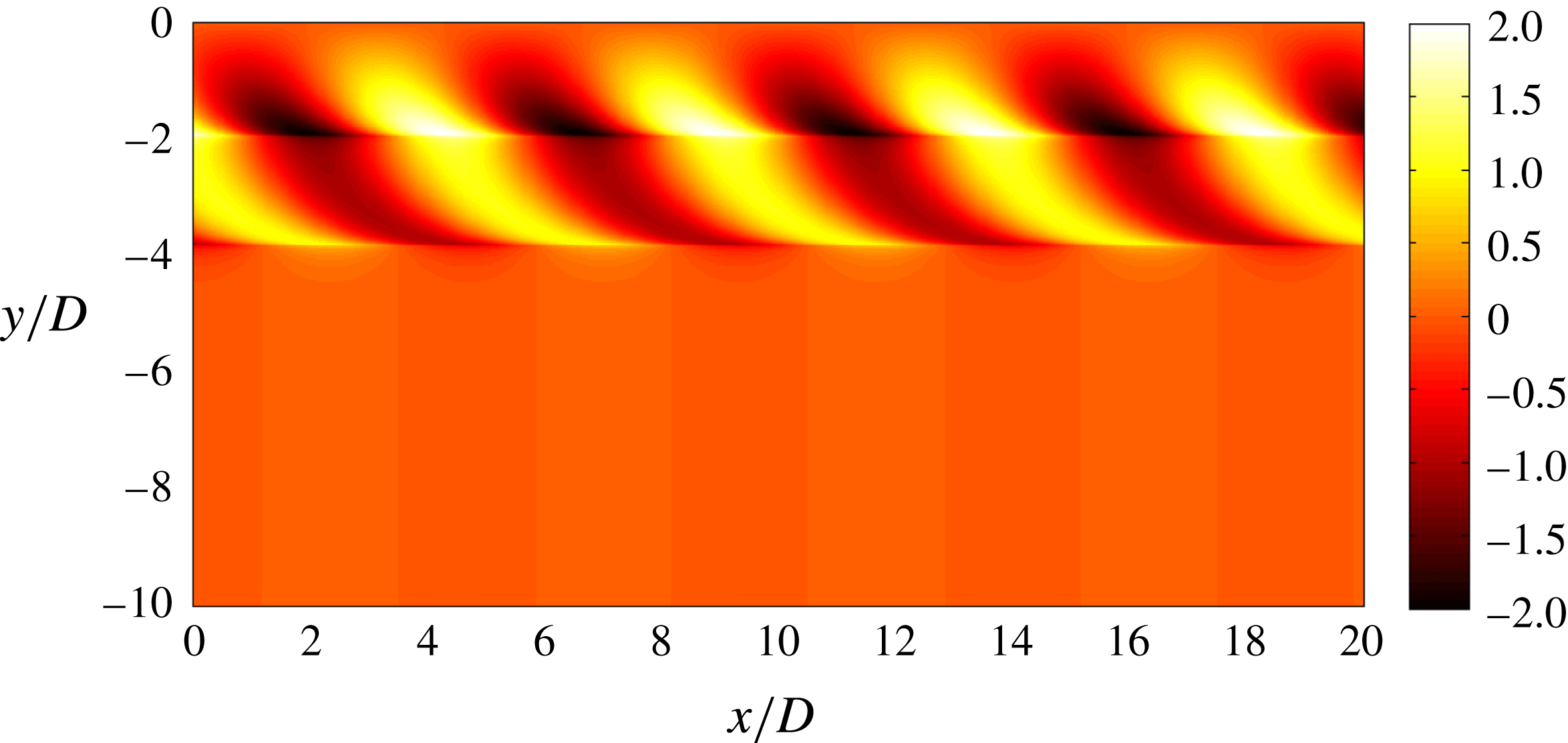
. The calculation, which makes use of the stationary phase method, is detailed in appendix D. This distribution is plotted in figure 20 two diameters above the wake for
 $F=8$
. It is composed of alternate lobes between
 $y/D=-1$
and
 $y/D=-4$
tilted at approximately
 $45^{\circ }$
with respect to the
 $x$
-axis. This structure is very similar to the internal waves measured experimentally at
 $Nt=16$
shown in figure 15(a). Moreover, the angle of
 $45^{\circ }$
is in excellent agreement with the measurements shown in figure 18. However, the theoretical solution does not spread in
 $y$
as much as in the experiments. This is probably because the pressure perturbation is broader in
 $y$
than the Dirac function taken theoretically in
 $y$
.
Analytical solution (4.8) of the internal waves emitted by a von Kármán vortex street two diameters above the wake.
 $F=8$
.

This pattern is closer to the experimental observations than the pattern obtained by Dupont & Voisin (Reference Dupont and Voisin1996) and Robey (Reference Robey1997). Indeed, the pattern is here invariant in the streamwise direction (as in the experiments) whereas the pattern obtained by Dupont & Voisin (Reference Dupont and Voisin1996) and Robey (Reference Robey1997) are localized behind the emitting point source.
4.6 Influence of the shape of the bluff body
Finally, the experiments done with a cylinder and a 6:1 spheroid have been analysed in the same way as for the sphere. The instantaneous spectra (in the frame moving at
 $U_{\unicode[STIX]{x1D719}}$
) have been used to extract the wavelength of the wake waves. It is plotted in figure 21(a) as a function of the Froude number and compared to the wavelength of the turbulent wake given by (4.2) at
 $Nt=30$
(dashed line). The wavelength of the cylinder is very close to the wavelength obtained for the sphere but it seems to be slightly larger (by approximately 20 %) for
 $F<20$
. As shown by Meunier & Spedding (Reference Meunier and Spedding2004), this can be explained for a self-preserved wake by the fact that the effective diameter of the turbulent wake is larger for a cylinder than for a sphere: it is 40 % larger when taken proportional to
 $\sqrt{C_{D}}$
. The wavelength should thus be 40 % larger but since the effective Froude number is also 30 % smaller (and since
 $\unicode[STIX]{x1D706}_{x}\sim F^{1/3}$
), the data for the cylinder can be expected to be 25 % above the sphere’s data in figure 21. This is in good agreement with the experimental results.
(a) Wavelength and (b) rescaled amplitude as a function of the Froude number. Symbols correspond to a sphere (
 $\circ$
), to a cylinder (▫) and to a 6:1 spheroid (▵). Large open symbols correspond to large bluff bodies (
 $Re\sim 600F$
) whereas small filled symbols correspond to small bluff bodies (
 $Re\sim 160F$
). In (a), the wavelength of the von Kármán vortex street (4.2) is plotted at
 $Nt=2$
(solid line) and at
 $Nt=30$
(dashed line). In (b), the dashed line corresponds to the prediction (4.6) for a sphere.

The wavelength of the slender spheroid is very close to the wavelength of the sphere for
 $F>20$
but it seems to be larger by approximately 40 % for
 $F<20$
. This result is counter-intuitive since the effective diameter of the spheroid is smaller than for the sphere and would give a wavelength approximately 20 % smaller. It is possible that the large aspect ratio of the spheroid creates initially a wake with a larger wavelength than for the sphere (in disagreement with the theory of self-preserved wakes). Meunier & Spedding (Reference Meunier and Spedding2004) indeed found experimentally that the wavelength of the spheroid’s vortex street is slightly larger (by approximately 15 %) at the beginning of their measurements (i.e.
 $Nt=100$
) but ultimately reaches the wavelength of the self-preserved turbulent wake at
 $Nt=200$
. This could explain the fact that the wavelength is 40 % larger than for the sphere at
 $Nt<30$
when the internal waves are emitted.
The amplitude of the internal waves is also measured for the cylinder and for the slender spheroid. It is plotted in figure 21(b). For the cylinder, the amplitude is very close to the amplitude obtained for the sphere on the whole range of Froude numbers. For the slender spheroid, the amplitude is approximately twice smaller for
 $F<20$
. This could be related to the fact that the wavelength is larger for these Froude numbers. Indeed, equation (4.4) indicates that the amplitude is proportional to the wavenumber squared (at constant isopycnal displacement
 $\unicode[STIX]{x1D701}$
) such that an increase of 40 % of the wavelength leads to an amplitude twice larger.
5 Conclusion
In this paper, we have analysed experimentally and theoretically the internal waves emitted by a bluff body translated horizontally in a continuously stratified fluid. Three different bluff bodies have been used: a sphere, a 6:1 cylinder and a 6:1 slender spheroid. Two types of internal waves are emitted and can be separated by averaging the velocity fields in the corresponding frame of reference.
First, lee internal waves are emitted by the bluff body itself. These large wavelength internal waves are stationary in the frame of reference of the bluff body. The wavelength is proportional to the Froude number and the amplitude of the vertical velocity gradient
 $\unicode[STIX]{x2202}w/\unicode[STIX]{x2202}z$
is inversely proportional to the Froude number. The scaling of the amplitude indicates that the lee internal waves cannot be predicted correctly by assuming that the flow has no separation behind the bluff body. It means that the separation of the flow, which is related to the drag force, creates a dominant contribution to the lee waves at large Froude numbers. A model derived from the Lighthill theory has been developed which describes the flow as a classical non-separating dipolar flow (proportional to the volume of the bluff body) superimposed to a recirculating jet (proportional to the drag force). This model clearly shows that the drag term is indeed larger than the volume term for
 $F>2$
(since the volume term leads to an amplitude
 $\unicode[STIX]{x2202}w/\unicode[STIX]{x2202}z$
scaling as
 $F^{-2}$
). It is curious to see that previous experimental studies on lee internal waves (see, e.g. Bonneton et al.
Reference Bonneton, Chomaz and Hopfinger1993; Robey Reference Robey1997) have been compared to theoretical models taking into account only the volume term. However these models were shown to be satisfactory for
 $F<2$
only, when the volume term is comparable to the drag term. This is why these studies deduced that the amplitude
 $\unicode[STIX]{x2202}w/\unicode[STIX]{x2202}z$
of the lee waves scales as
 $F^{-2}$
(or equivalently that the amplitude
 $\unicode[STIX]{x1D701}$
of the isopycnal displacement scales as
 $F^{-1}$
). In fact, at larger Froude numbers, the drag term becomes dominant and leads to an amplitude
 $\unicode[STIX]{x2202}w/\unicode[STIX]{x2202}z$
scaling as
 $F^{-1}$
(or equivalently an amplitude
 $\unicode[STIX]{x1D701}$
independent of
 $F$
). It should be noted that the spatial structure of the drag modes and the volume modes are very similar and simply in phase quadrature.
Second, wake waves are emitted by the turbulent wake at a smaller wavelength. As noted by Robey (Reference Robey1997), these waves move at a velocity
 $U_{\unicode[STIX]{x1D719}}$
much smaller than the bluff body velocity and scaling as
 $F^{-2/3}$
. This velocity quantitatively corresponds to the defect velocity of the wake at the beginning of the NEQ regime (
 $Nt=2$
), i.e. when the local Froude number is equal to 1. Furthermore, the wavelength of the internal waves scales as
 $F^{1/3}$
as already noted by Spedding et al. (Reference Spedding, Browand, Bell, Chen, Lawrence, Pieters and Yonemitsu2000) and Abdilghanie & Diamessis (Reference Abdilghanie and Diamessis2013). The streamwise wavelength is quantitatively equal to the wavelength of the von Kármán vortex street at
 $Nt=30$
(defined as the distance between co-rotating vortices). These observations indicate that the wake waves are emitted by the travelling coherent structures in the transonic stage. A simplified model has been done where the von Kármán vortex street is modelled as a double row of periodic pressure perturbations. This model is close to the model proposed by Robey (Reference Robey1997) of a single travelling vortex or the model of Dupont & Voisin (Reference Dupont and Voisin1996) of an oscillating point source. The spatial structure of the waves emitted by the vortex street is derived analytically and presents strong similarities with the wake waves observed experimentally. However, the amplitude of the wake waves has not been predicted theoretically. Experimentally, the amplitude seems to depend on the Reynolds number (in contrast to the lee waves which are Reynolds number independent). The empirical scaling for the amplitude is
 $\unicode[STIX]{x2202}w/\unicode[STIX]{x2202}z\sim Re^{0.4}F^{-0.8}$
in fair agreement with the numerical results of Abdilghanie & Diamessis (Reference Abdilghanie and Diamessis2013).
The dominance of the drag term in the lee internal waves may have strong implications for geophysical flows. First, it means that the amplitude is much larger than obtained with the volume term only at moderate to large Froude numbers.
Second, it means that all the internal waves emitted by a bluff body can be quantified simply by the drag of the bluff body. Indeed, the wake waves simply depends on the effective diameter of the bluff body, i.e. to the square root of the drag coefficient. The shape of the bluff body is thus only relevant through the amount of drag that it creates. This permits to draw a very simple picture of emitted internal waves depending on a single parameter, as shown here for three different bluff bodies. This would be very useful in weather forecast models for example since the bottom drag is usually known even for very complex topography.
Third, it implies that internal waves emitted at large Froude numbers by a self-propelled bluff body may be much weaker than for a towed body. Indeed, the drag term in the lee waves should vanish and the amplitude of the wake waves should be smaller since the amplitude and velocity of the von Kármán vortex street is smaller. It would be interesting to check experimentally if this statement is correct. For a self-propelled body, the amplitude of the lee internal waves can be predicted by the volume term. But the amplitude of the wake waves still remains unknown. It is even unclear whether the coherent vortices present in a turbulent momentumless wake can emit internal waves since they may not move in the streamwise direction. Further research on this type of wake is clearly needed in order to draw a confident picture of the emitted internal waves.
Acknowledgements
All the experiments have been done at Univ. Southern California with the support of ONR grant no. N00014-96-1-0001 under Dr L. P. Purtell and Dr R. Joslin. Reviewer 2 is greatly acknowledged for correcting several errors in the formulae and in the figures.
Appendix A. Derivation of the amplitude of the lee internal waves
The goal of this section is to solve (3.4) with the source terms
 ${\mathcal{Q}}$
given by (3.2) and
 ${\mathcal{F}}$
by (3.3). The right-hand side term in (3.4), is moving at the velocity
 $-U_{B}$
such that it can be written
 ${\mathcal{S}}(X,y,z)$
with
 $X=x+U_{B}t$
. The velocity
 $w$
is considered to be a function of
 $X$
,
 $y$
and
 $z$
in order to describe a stationary solution in the frame of reference moving with the bluff body. Temporal derivatives
 $\unicode[STIX]{x2202}/\unicode[STIX]{x2202}t$
are thus replaced by
 $U_{B}\unicode[STIX]{x2202}/\unicode[STIX]{x2202}X$
in these new variables. Taking the double Fourier transform over
 $X$
and
 $y$
gives
 $$\begin{eqnarray}{\mathcal{D}}(-k_{X}U_{B},\boldsymbol{k})\tilde{w}(k_{X},k_{y},z)=-k_{X}^{2}U_{B}^{2}\displaystyle \frac{\unicode[STIX]{x2202}\tilde{{\mathcal{Q}}}}{\unicode[STIX]{x2202}z}-k_{X}^{2}U_{B}\displaystyle \frac{\unicode[STIX]{x2202}\tilde{{\mathcal{F}}_{x}}}{\unicode[STIX]{x2202}z},\end{eqnarray}$$
where
 $$\begin{eqnarray}{\mathcal{D}}(\unicode[STIX]{x1D714},\boldsymbol{k})=-\unicode[STIX]{x1D714}^{2}\left(-k_{X}^{2}-k_{y}^{2}+\displaystyle \frac{\unicode[STIX]{x2202}^{2}}{\unicode[STIX]{x2202}z^{2}}\right)-N^{2}(k_{X}^{2}+k_{y}^{2})\end{eqnarray}$$
is the dispersion relation of the internal waves. In (A 1), the frequency has been taken equal to the Doppler shift
 $-k_{X}U_{B}$
since the source terms are stationary in the frame moving at the velocity
 $-U_{B}$
.
The velocity is then decomposed into eigenmodes
 $$\begin{eqnarray}w=\mathop{\sum }_{n}w_{n}(X,y)\unicode[STIX]{x1D713}_{n}(z)\end{eqnarray}$$
of the dispersion equation in the vertical direction. Since the buoyancy frequency is constant, the eigenmodes are simply sine functions in
 $z$
. The requirement of the vanishing velocity at
 $z=0$
and
 $z=H$
and the orthonormality of the set of eigenmodes imposes:
 $$\begin{eqnarray}\unicode[STIX]{x1D713}_{n}(z)=\sqrt{\frac{2}{H}}\sin \left(\frac{n\unicode[STIX]{x03C0}z}{H}\right).\end{eqnarray}$$
Introducing the decomposition (A 3) in (A 1), multiplying by
 $\unicode[STIX]{x1D713}_{n}(z)$
and integrating over
 $z$
leads to the formula
 $$\begin{eqnarray}\tilde{w}_{n}(k_{X},k_{y})=\frac{{\mathcal{P}}_{n}(k_{X},k_{y})}{{\mathcal{D}}_{n}(-k_{X}U_{B},k_{X},k_{y})},\end{eqnarray}$$
where
 $$\begin{eqnarray}{\mathcal{P}}_{n}(k_{X},k_{y})=\int _{z=0}^{H}\unicode[STIX]{x1D713}_{n}(z)\left[-k_{X}^{2}U_{B}^{2}\displaystyle \frac{\unicode[STIX]{x2202}\tilde{{\mathcal{Q}}}}{\unicode[STIX]{x2202}z}-k_{X}^{2}U_{B}\displaystyle \frac{\unicode[STIX]{x2202}\tilde{{\mathcal{F}}_{x}}}{\unicode[STIX]{x2202}z}\right]\,\text{d}z\end{eqnarray}$$
is the scalar product of the source terms with the eigenmode
 $\unicode[STIX]{x1D713}_{n}(z)$
and
 $$\begin{eqnarray}{\mathcal{D}}_{n}(\unicode[STIX]{x1D714},k_{X},k_{y})=\unicode[STIX]{x1D714}^{2}\left(k_{X}^{2}+k_{y}^{2}+\frac{n^{2}\unicode[STIX]{x03C0}^{2}}{H^{2}}\right)-N^{2}(k_{X}^{2}+k_{y}^{2})\end{eqnarray}$$
is the dispersion relation of the mode with vertical wavenumber
 $n\unicode[STIX]{x03C0}/H$
.
The scalar product term is calculated using an integration by parts:
 $$\begin{eqnarray}{\mathcal{P}}_{n}(k_{X},k_{y})=\unicode[STIX]{x1D713}_{n}^{\prime }(z_{0})\left[\text{i}k_{X}^{3}U_{B}^{3}\left(\frac{D}{2}\right)^{3}+k_{X}^{2}\frac{\unicode[STIX]{x03C0}C_{D}U_{B}^{3}D^{2}}{8}\right].\end{eqnarray}$$
The Fourier transform
 $\tilde{w}_{n}(k_{X},k_{y})$
of the velocity contains two poles for each wavenumber
 $k_{X}$
at
 $$\begin{eqnarray}k_{y}=\pm k_{y}^{0}(k_{X})=\pm k_{X}\sqrt{\frac{\hat{n}^{2}F^{2}-1+(U_{B}k_{X}/N)^{2}}{1-(U_{B}k_{X}/N)^{2}}},\end{eqnarray}$$
where
 $$\begin{eqnarray}\hat{n}=\frac{n\unicode[STIX]{x03C0}D}{2H}.\end{eqnarray}$$
However, for causality conditions, only the positive (respectively negative) pole
 $+k_{y}^{0}(k_{X})$
must be taken into account in the inverse Fourier transform when
 $y>0$
(respectively
 $y<0$
). Using the residue theorem, the inverse Fourier transform over
 $k_{y}$
can be calculated, leading to
 $$\begin{eqnarray}\tilde{w}(k_{X},y,z)=-\frac{\text{i}}{2}\mathop{\sum }_{n}\frac{\unicode[STIX]{x1D713}_{n}(z)}{N^{2}-U_{B}^{2}k_{X}^{2}}\frac{\text{e}^{\text{i}k_{y}^{0}(k_{X})|y|}}{k_{y}^{0}(k_{X})}{\mathcal{P}}_{n}(k_{X},k_{y}^{0}).\end{eqnarray}$$
Taking the inverse Fourier transform over
 $k_{X}$
with a change of variable
 $s=U_{B}k_{X}/N$
leads to the vertical velocity in real space:
 $$\begin{eqnarray}w(X,y,z)=\frac{-\text{i}}{4\unicode[STIX]{x03C0}N^{2}}\mathop{\sum }_{n}\unicode[STIX]{x1D713}_{n}(z)\int _{-\infty }^{+\infty }\frac{\text{e}^{\text{i}k_{y}^{0}|y|}\text{e}^{\text{i}sXN/U_{B}}}{|s|\sqrt{1-s^{2}}\sqrt{\hat{n}^{2}F^{2}-(1-s^{2})}}{\mathcal{P}}_{n}(Ns/U_{B},k_{y}^{0})\,\text{d}s.\end{eqnarray}$$
Causality (group velocity) considerations show that the doubly infinite integral along the
 $s$
-axis must be taken below all singularities appearing on the real
 $s$
-axis for the downstream (
 $X>0$
) field. In this regard, inspection of (A 12) reveals that the integrand has branch point singularities at
 $s=\pm 1$
and
 $s=\pm s_{n}=\pm \sqrt{1-\hat{n}^{2}F^{2}}$
for subcritical modes. Of course, a branch point also exists at
 $s=0$
, but this singularity is associated with the potential-like (near-field) motion, making no contribution to the radiated wave field, and will be disregarded. Then, by Cauchy’s theorem, and the fact that the contour for
 $X>0$
must be closed in the upper half of the complex
 $s$
-plane, the integral can be reduced to contours around branch cuts taken on the real axis between
 $(-1,-s_{n})$
and between
 $(+s_{n},+1)$
. By symmetry properties of the integrand, the two resulting integral expressions arising from the two separate branch cut contours can be combined into just a single integral over the finite interval
 $(s_{n},1)$
. For supercritical modes, the integral can be reduced to a contour around the branch cut taken on the real axis between
 $(0,1)$
.
Furthermore, the combination of complex exponential terms are readily reduced to an entirely real expression with purely trigonometric variation in the horizontal
 $(X,y)$
plane. By this means the solution for the vertical velocity field for the linear, radiated wave pattern emanating from the volumetric and drag force sources can be represented by the following expression involving a single quadrature plus a final summation over the discrete set of vertical eigenmodes:
 $$\begin{eqnarray}\displaystyle & & \displaystyle w(X,y,z)=\mathop{\sum }_{n}\unicode[STIX]{x1D713}_{n}(z)\unicode[STIX]{x1D713}_{n}^{\prime }(z_{0})\nonumber\\ \displaystyle & & \displaystyle \quad \times \,\int _{s_{n}}^{1}\frac{\cos (k_{y}^{0}|y|)\displaystyle \left[\frac{-ND^{3}}{\unicode[STIX]{x03C0}}s^{2}\cos \left(\frac{sXN}{U_{B}}\right)-C_{D}U_{B}D^{2}s\sin \left(\frac{sXN}{U_{B}}\right)\right]}{\displaystyle 8\sqrt{1-s^{2}}\sqrt{\hat{n}^{2}F^{2}-(1-s^{2})}}\,\text{d}s,\qquad\end{eqnarray}$$
where
 $s_{n}=0$
for supercritical modes and
 $s_{n}=\sqrt{1-\hat{n}^{2}F^{2}}$
for subcritical modes. Introducing the expression (A 9) of the pole
 $k_{y}^{0}$
and the expression of
 $\unicode[STIX]{x1D713}_{n}(z)$
leads to the formula (3.6) for the vertical velocity
 $w$
.
The volume mode
 $I_{n}^{vol}$
and the drag mode
 $I_{n}^{drag}$
(defined by (3.7) and (3.8) respectively) are plotted in figure 22 for
 $F=4$
,
 $H/D=10.2$
and
 $n=4$
. They exhibit hyperbolic phase lines because these modes are supercritical (since
 $\hat{n}F=n\unicode[STIX]{x03C0}DF/(2H)=2.46$
is larger than 1). This means that the velocity of the bluff body is larger than the maximum phase velocity for this vertical wavenumber.
Structure of (a) the volume mode
 $I_{n}^{vol}(X,y)$
and (b) the drag mode
 $I_{n}^{drag}(X,y)$
defined by (3.7) and (3.8) respectively for
 $n=4$
. Here
 $F=4$
and
 $h=H/D=10.2$
such that the mode is supercritical for
 $n=4$
(defined by
 $k_{z}=n\unicode[STIX]{x03C0}/H$
) since
 $\hat{n}F=n\unicode[STIX]{x03C0}U_{B}/NH=2.46$
is larger than 1.

If the vertical wavenumber is decreased, the phase velocity may exceed the bluff body velocity if
 $\hat{n}F<1$
. In this case, the modes become subcritical with a different spatial structure, as shown in figure 23.
Structure of the volume mode
 $I_{n}^{vol}(X,y)$
defined by (3.7) for
 $n=1$
. Here,
 $F=4$
and
 $h=H/D=10.2$
such that the mode is subcritical for
 $n=1$
(defined by
 $k_{z}=n\unicode[STIX]{x03C0}/H$
) since
 $\hat{n}F=n\unicode[STIX]{x03C0}U_{B}/NH=0.61$
is smaller than 1.

Appendix B. Stationary phase approximation
The integrals
 $I_{n}(X,y)$
are very difficult to integrate because they strongly oscillate for large
 $X$
or
 $y$
. They can be approximated using the stationary phase method. For example, the volume integral given in (3.7) can be written as:
 $$\begin{eqnarray}I_{n}^{vol}(X,y)=\mathop{\sum }_{\unicode[STIX]{x1D716}=\pm 1}\int _{0}^{1}f(s)\cos [g_{\unicode[STIX]{x1D716}}(s)]\,\text{d}s,\end{eqnarray}$$
with
 $$\begin{eqnarray}\displaystyle & \displaystyle f(s)=\frac{s^{2}}{2\sqrt{1-s^{2}}\sqrt{\hat{n}^{2}-F^{-2}(1-s^{2})}} & \displaystyle\end{eqnarray}$$
 $$\begin{eqnarray}\displaystyle & \displaystyle g_{\unicode[STIX]{x1D716}}(s)=\frac{2s}{FD}\left(X+\unicode[STIX]{x1D716}y\sqrt{\frac{\hat{n}^{2}F^{2}}{1-s^{2}}-1}\right)\quad \text{where }X=x+U_{B}t. & \displaystyle\end{eqnarray}$$
The derivative of the phase
 $g^{\prime }(s)$
vanishes when
 $\unicode[STIX]{x1D716}$
has the sign of
 $-y$
(for
 $X>0$
) and when
 $s=\sqrt{1-\unicode[STIX]{x1D707}}$
with
 $\unicode[STIX]{x1D707}$
solution of
 $$\begin{eqnarray}\unicode[STIX]{x1D707}^{4}\left(1+\frac{X^{2}}{y^{2}}\right)-\hat{n}^{2}F^{2}\frac{X^{2}}{y^{2}}\unicode[STIX]{x1D707}^{3}-2\hat{n}^{2}F^{2}\unicode[STIX]{x1D707}^{2}+\hat{n}^{4}F^{4}=0\end{eqnarray}$$
in the interval
 $[0,1]$
. Calculating the second derivative of the phase
 $g^{\prime \prime }(s)$
and introducing in the approximation for large
 $x$
,
 $y$
leads to a simple value of the integral:
 $$\begin{eqnarray}I_{n}^{vol}(X,y)=\frac{\sqrt{\unicode[STIX]{x03C0}U_{B}}(\hat{n}^{2}F^{2}-\unicode[STIX]{x1D707})^{1/4}(\unicode[STIX]{x1D707}-\unicode[STIX]{x1D707}^{2})^{3/4}}{\sqrt{NH}\sqrt{2\hat{n}^{2}y|3\hat{n}^{2}F^{2}+\unicode[STIX]{x1D707}(\unicode[STIX]{x1D707}-4)|}}\cos (\unicode[STIX]{x1D719}),\end{eqnarray}$$
with
 $$\begin{eqnarray}\unicode[STIX]{x1D719}=\frac{2\sqrt{1-\unicode[STIX]{x1D707}}}{DF}\left(X+U_{B}t-|y|\sqrt{\hat{n}^{2}F^{2}/\unicode[STIX]{x1D707}-1}-\unicode[STIX]{x1D716}^{\prime }\frac{\unicode[STIX]{x03C0}}{4}\right)\end{eqnarray}$$
and
 $$\begin{eqnarray}\unicode[STIX]{x1D716}^{\prime }=\text{sign}[\,y(3\hat{n}^{2}F^{2}+\unicode[STIX]{x1D707}(\unicode[STIX]{x1D707}-4))].\end{eqnarray}$$
For subcritical modes, the root
 $\unicode[STIX]{x1D707}$
must also be smaller than
 $\hat{n}^{2}F^{2}$
.
For drag modes, the same type of calculation gives the result:
 $$\begin{eqnarray}I_{n}^{drag}(X,y)=\frac{\sqrt{\unicode[STIX]{x03C0}U_{B}}(\hat{n}^{2}F^{2}-\unicode[STIX]{x1D707})^{1/4}(\unicode[STIX]{x1D707}-\unicode[STIX]{x1D707}^{2})^{3/4}}{\sqrt{NH}\sqrt{2\hat{n}^{2}y|3\hat{n}^{2}F^{2}+\unicode[STIX]{x1D707}(\unicode[STIX]{x1D707}-4)|}\sqrt{1-\unicode[STIX]{x1D707}}}\sin (\unicode[STIX]{x1D719}).\end{eqnarray}$$
The final result for the velocity takes a form without integrals:
 $$\begin{eqnarray}\displaystyle \frac{w}{U} & = & \displaystyle -\left(\frac{D}{2H}\right)^{2}\mathop{\sum }_{n=1}^{\infty }\frac{\sqrt{\unicode[STIX]{x03C0}U_{B}}(\hat{n}^{2}F^{2}-\unicode[STIX]{x1D707})^{1/4}(\unicode[STIX]{x1D707}-\unicode[STIX]{x1D707}^{2})^{3/4}}{\sqrt{NH}\sqrt{2\hat{n}^{2}y|3\hat{n}^{2}F^{2}+\unicode[STIX]{x1D707}(\unicode[STIX]{x1D707}-4)|}}\nonumber\\ \displaystyle & & \displaystyle \times \,\left(\frac{2\cos (\unicode[STIX]{x1D719})}{\unicode[STIX]{x03C0}F^{2}}+\frac{C_{D}\sin (\unicode[STIX]{x1D719})}{F\sqrt{1-\unicode[STIX]{x1D707}}}\right)n\unicode[STIX]{x03C0}\sin \left(\frac{n\unicode[STIX]{x03C0}z}{H}\right)\cos \left(\frac{n\unicode[STIX]{x03C0}z_{0}}{H}\right),\end{eqnarray}$$
where
 $\unicode[STIX]{x1D719}$
is given by (B 6) and
 $\unicode[STIX]{x1D707}$
is the root of (B 4) in the interval
 $[0,\min (1,\hat{n}^{2}F^{2})]$
. If there are several roots in this interval, the velocity is the sum of all the terms corresponding to each root. This solution is compared in figure 24 with the exact value of the integral and gives an excellent agreement far from the bluff body, i.e. for
 $X>10D$
. However, this solution diverges at the cusp of the subcritical modes. The correct amplitude at the cusped edge of wave field for subcritical modes requires evaluation of the solution involving a higher-order stationary point that arises when both
 $g^{\prime }(s)$
and
 $g^{\prime \prime }(s)$
vanish. The analysis of this case has not been performed, and hence this stationary phase approximation has not been used throughout the paper. All the theoretical results shown in the paper are obtained by computing numerically the integral of the full solution (A 13).
Comparison of the vertical velocity gradient
 $\unicode[STIX]{x2202}w/\unicode[STIX]{x2202}z$
obtained by the exact theory (dashed line) and by the approximation using the stationary phase method (solid line). This is obtained for a sphere with
 $F=4$
,
 $h=H/D=10.2$
.
 $z/H=0.629$
and
 $z_{0}/H=0.435$
.

Appendix C. Additional effects
C.1 Finite size source
The finite size of the bluff body may be taken into account by supposing that the source is distributed over a disk located at
 $X=0$
with a characteristic size
 $a$
(close to the diameter of the bluff body). Mathematically, it can be done by replacing the Dirac functions
 $\unicode[STIX]{x1D6FF}(y)$
and
 $\unicode[STIX]{x1D6FF}(z-z_{0})$
in the source terms of (3.2), (3.3) by Gaussian distributions
 $\unicode[STIX]{x1D6FF}_{a}(y)=\exp (-y^{2}/a^{2})/(a\sqrt{\unicode[STIX]{x03C0}})$
and
 $\unicode[STIX]{x1D6FF}_{a}(z-z_{0})=\exp [-(z-z_{0})^{2}/a^{2}]/(a\sqrt{\unicode[STIX]{x03C0}})$
.
The first modification to the calculation is that the scalar product
 ${\mathcal{P}}_{n}(k_{X},k_{y})$
obtained in (A 8) is multiplied by an additional term corresponding to the Fourier transform of
 $\unicode[STIX]{x1D6FF}_{a}(y)$
which is equal to
 $\exp (-k_{y}^{2}a^{2}/4)$
. This term is taken at
 $k_{y}=k_{y}^{0}$
given by (A 9) after the application of the residue theorem and thus becomes
 $$\begin{eqnarray}\exp \left[\frac{-s^{2}}{4}\left(\frac{\hat{n}^{2}F^{2}-(1-s^{2})}{1-s^{2}}\right)\frac{a^{2}}{H^{2}}\right]\end{eqnarray}$$
after the change of variable.
The second modification is due to the finite vertical size. For a point source, the integral over
 $z$
in the scalar product
 ${\mathcal{P}}_{n}(k_{X},k_{y})$
is equal to
 $$\begin{eqnarray}\int _{z=0}^{H}\unicode[STIX]{x1D713}_{n}(z)\frac{\text{d}}{\text{d}z}[\unicode[STIX]{x1D6FF}(z-z_{0})]\,\text{d}z=-\unicode[STIX]{x1D713}_{n}^{\prime }(z0).\end{eqnarray}$$
In the case of a finite size source
 $\unicode[STIX]{x1D6FF}_{a}(z-z_{0})$
, this integral is thus replaced (using an integration by part) by
 $$\begin{eqnarray}-\int _{z=0}^{H}\unicode[STIX]{x1D713}_{n}^{\prime }(z)\unicode[STIX]{x1D6FF}_{a}(z-z_{0})\,\text{d}z.\end{eqnarray}$$
In the limit where
 $H$
is much larger than the size
 $a$
, the function
 $\unicode[STIX]{x1D6FF}_{a}(z-z_{0})$
is very small for
 $z<0$
and for
 $z>H$
such that the bounds of the integral can be extended from
 $-\infty$
to
 $+\infty$
. In this case, the integral can be calculated analytically using the form of
 $\unicode[STIX]{x1D713}_{n}(z)$
given by (A 4) as:
 $$\begin{eqnarray}-\unicode[STIX]{x1D713}_{n}^{\prime }(z_{0})\exp \left[-\frac{1}{4}\left(\frac{n\unicode[STIX]{x03C0}a}{H}\right)^{2}\right].\end{eqnarray}$$
However, if the bluff body is located at a node of mode
 $n$
(i.e. if
 $\cos (n\unicode[STIX]{x03C0}z_{0}/H)=0$
), this integral vanishes at first order in
 $a/H$
and the second order must be calculated leading to an additional term equal to
 $$\begin{eqnarray}\frac{n\unicode[STIX]{x03C0}}{H}\sqrt{\frac{2}{H}}\sin \left(\frac{n\unicode[STIX]{x03C0}z_{0}}{H}\right)\int _{\unicode[STIX]{x1D719}=z_{0}/a}^{\unicode[STIX]{x1D719}=(H-z_{0})/a}\sin \left(\frac{n\unicode[STIX]{x03C0}a\unicode[STIX]{x1D719}}{H}\right)\text{e}^{-\unicode[STIX]{x1D719}^{2}}\,\text{d}\unicode[STIX]{x1D719}.\end{eqnarray}$$
Experimentally, the bluff body is always located close to the mid-height (but not exactly at mid-height) such that the first-order term is always dominant for the first modes.
To conclude, the effect of the finite size of the bluff body can be taken into account by multiplying the integrand in (3.7), (3.8) by
 $$\begin{eqnarray}\exp \left[\frac{-s^{2}}{4}\left(\frac{\hat{n}^{2}F^{2}-(1-s^{2})}{1-s^{2}}\right)\frac{a^{2}}{H^{2}}\right]\exp \left[-\frac{1}{4}\left(\frac{n\unicode[STIX]{x03C0}a}{H}\right)^{2}\right].\end{eqnarray}$$
In the following, we will suppose that the Gaussian size of the distribution
 $\unicode[STIX]{x1D6FF}_{a}$
is equal to the radius of the bluff body (
 $a=D/2$
). In (C 6), the first exponential term
 $\exp (-k_{y}^{2}a^{2}/4)$
is of the order of
 $\exp (-a^{2}/(FD)^{2})$
if
 $k_{y}$
is taken of the order of
 $k_{X}\sim 2/F$
. This term is thus close to 1 for
 $F$
larger than 1. The second term is also close to 1 in the experiments for the first modes since
 $a/H$
is always smaller than 0.05. The higher modes (for
 $n>5$
) may be attenuated by this second term. However, in our experiments, the Reynolds number is not large enough so that the viscous attenuation of these higher modes is larger than the attenuation due to the finite size of the bluff body. Indeed, the viscous attenuation is larger than the finite size attenuation when
 $X/D\gg Re/64$
which means that in our experiments, the viscous attenuation is dominant for
 $X/D$
larger than approximately 20. We have checked that the theoretical predictions taking into account the finite size of the bluff body was close to the predictions without the finite size within approximately 10 %. This is why this effect has not been taken into account in the core of the paper. However, this effect will be dominant (larger than the viscous effect) for larger Reynolds numbers, i.e. in geophysical and naval applications.
C.2 Non-Boussinesq effects
The non-Boussinesq effects can be taken into account in the calculation. The final formula for the velocity
 $w$
is simply obtained from (A 13) while replacing
 $\unicode[STIX]{x1D713}_{n}^{\prime }(z_{0})$
by
 $$\begin{eqnarray}\unicode[STIX]{x1D713}_{n}^{\prime }(z_{0})+\frac{\unicode[STIX]{x1D6E5}}{H\sqrt{2H}}\left[n\unicode[STIX]{x03C0}\frac{z+z_{0}-H}{H}\cos \left(\frac{n\unicode[STIX]{x03C0}z_{0}}{H}\right)-\sin \left(\frac{n\unicode[STIX]{x03C0}z_{0}}{H}\right)\right]\end{eqnarray}$$
for the volume mode and by
 $$\begin{eqnarray}\unicode[STIX]{x1D713}_{n}^{\prime }(z_{0})+\frac{\unicode[STIX]{x1D6E5}}{H\sqrt{2H}}\left[n\unicode[STIX]{x03C0}\frac{z+3z_{0}-2H}{H}\cos \left(\frac{n\unicode[STIX]{x03C0}z_{0}}{H}\right)+\sin \left(\frac{n\unicode[STIX]{x03C0}z_{0}}{H}\right)\right]\end{eqnarray}$$
for the drag mode. Here,
 $\unicode[STIX]{x1D6E5}=(\unicode[STIX]{x1D70C}_{bottom}-\unicode[STIX]{x1D70C}_{top})/\unicode[STIX]{x1D70C}_{average}$
quantifies the non-Boussinesq effect. In our experiments, this parameter
 $\unicode[STIX]{x1D6E5}$
is always smaller than 0.1 such that the non-Boussinesq are always smaller than 10 %.
C.3 Free surface effect
The goal of this subsection is to calculate the dispersion relation of internal waves coupled to surface waves in order to derive the correction on the internal modes. The eigenmodes
 $\unicode[STIX]{x1D713}_{n}$
are solutions of the dispersion equation:
 $$\begin{eqnarray}\unicode[STIX]{x1D713}_{n}^{\prime \prime }+k_{H}^{2}\left(\frac{N^{2}}{\unicode[STIX]{x1D714}^{2}}-1\right)\unicode[STIX]{x1D713}_{n}=0,\end{eqnarray}$$
with boundary conditions
 $$\begin{eqnarray}\unicode[STIX]{x1D713}_{n}(z=0)=0\quad \text{and}\quad \unicode[STIX]{x1D713}_{n}(z=H)=\frac{\unicode[STIX]{x1D6FF}\unicode[STIX]{x1D714}^{2}}{HN^{2}k_{H}^{2}}\unicode[STIX]{x1D713}_{n}^{\prime }(z=H),\end{eqnarray}$$
where
 $\unicode[STIX]{x1D6FF}=N^{2}H/g$
is a small parameter and
 $k_{H}=(k_{X}^{2}+k_{y}^{2})^{1/2}$
is the horizontal wavevector. The eigenmodes are sine functions
 $$\begin{eqnarray}\unicode[STIX]{x1D713}_{n}(z)=\sqrt{\frac{2}{H}}\sin (k_{z}z),\end{eqnarray}$$
with the vertical wavenumber given by
 $$\begin{eqnarray}k_{z}=\frac{n\unicode[STIX]{x03C0}}{H}+\unicode[STIX]{x1D6FF}n\unicode[STIX]{x03C0}\frac{\unicode[STIX]{x1D714}^{2}}{N^{2}H^{3}k_{H}^{2}}\end{eqnarray}$$
in order to respect the boundary conditions at first order. Introducing this solution
 $\unicode[STIX]{x1D713}_{n}$
into the dispersion equation (C 9) leads to the dispersion relation at first order in
 $\unicode[STIX]{x1D6FF}$
:
 $$\begin{eqnarray}\unicode[STIX]{x1D714}^{2}=\frac{k_{H}^{2}}{k_{H}^{2}+n^{2}\unicode[STIX]{x03C0}^{2}/H^{2}}\left(1-\frac{2\unicode[STIX]{x1D6FF}}{n^{2}\unicode[STIX]{x03C0}^{2}}\right).\end{eqnarray}$$
The pole
 $k_{y}^{0}$
of the dispersion relation can then be obtained at first order in
 $\unicode[STIX]{x1D6FF}$
. Using the change of variable
 $s=FHk_{X}$
, it can be written
 $$\begin{eqnarray}k_{y}^{0}=|s|\sqrt{\frac{\hat{n}^{2}F^{2}-[(1-\unicode[STIX]{x1D6E5}_{n})-s^{2}]}{(1-\unicode[STIX]{x1D6E5}_{n})-s^{2}}}\quad \text{with }\unicode[STIX]{x1D6E5}_{n}=\frac{2\unicode[STIX]{x1D6FF}}{(n\unicode[STIX]{x03C0})^{2}}.\end{eqnarray}$$
To conclude, the effect of the free surface can be added in the volume and drag modes of (3.7), (3.8) by replacing
 $(1-s^{2})$
by
 $([1-\unicode[STIX]{x1D6E5}_{n}]-s^{2})$
where
 $\unicode[STIX]{x1D6E5}_{n}=2N^{2}H/(gn^{2}\unicode[STIX]{x03C0}^{2})$
. In our experiments, this effect simply translates the modes in
 $x$
by approximately a quarter of wavelength. It does not modify significantly the amplitude, wavelength and spreading angle of the modes. This is why this effect has not been taken into account in the core of the paper.
Vertical velocity gradient obtained by the viscous model (grey/red) and the inviscid model (black) as a function of the number of modes
 $n$
. In (a), the velocity gradient is obtained for a single mode
 $n$
. In (b) the velocity gradient is cumulated for modes
 $1{-}n$
.
 $F=4$
,
 $h=H/D=10.2$
.
 $z/H=0.629$
,
 $z_{0}/H=0.435$
,
 $X/FD=11$
and
 $y/D=-10$
.

Appendix D. Internal waves emitted by a von Kármán vortex street
The goal of this section is to calculate the internal waves emitted by a double row of alternate vortices which create a pressure perturbation at
 $z=z_{0}$
given by (4.7). For a single row of vortices located at
 $y=+d/2$
, the pressure is searched as:
 $$\begin{eqnarray}p=\tilde{p}({\tilde{y}},\tilde{z})\cos (k_{x}x-\unicode[STIX]{x1D714}t)\quad \text{with }\left\{\begin{array}{@{}l@{}}\unicode[STIX]{x1D714}=-k_{x}U_{\unicode[STIX]{x1D719}}\\ {\tilde{y}}=y-d/2\\ \tilde{z}=z-z_{0}.\end{array}\right.\end{eqnarray}$$
The pressure is subject to the boundary condition
 $\tilde{p}=p_{0}\unicode[STIX]{x1D6FF}({\tilde{y}})$
at
 $\tilde{z}=0$
. The dispersion equation of internal waves leads to the equation for
 $\tilde{p}$
 $$\begin{eqnarray}\left(\displaystyle \frac{\unicode[STIX]{x2202}^{2}}{\unicode[STIX]{x2202}{\tilde{y}}^{2}}+\displaystyle \frac{\unicode[STIX]{x2202}^{2}}{\unicode[STIX]{x2202}\tilde{z}^{2}}-k_{x}^{2}\right)\tilde{p}-\frac{N^{2}}{\unicode[STIX]{x1D714}^{2}}\left(\displaystyle \frac{\unicode[STIX]{x2202}^{2}}{\unicode[STIX]{x2202}{\tilde{y}}^{2}}-k_{x}^{2}\right)\tilde{p}=0.\end{eqnarray}$$
The Fourier transform in
 ${\tilde{y}}$
leads to the solution
 $$\begin{eqnarray}\tilde{p}=\frac{p_{0}}{2\unicode[STIX]{x03C0}}\int _{-\infty }^{+\infty }\text{e}^{\text{i}k_{y}{\tilde{y}}}\text{e}^{\text{i}\sqrt{(N^{2}/\unicode[STIX]{x1D714}^{2}-1)(k_{x}^{2}+k_{y}^{2})}\tilde{z}}\,\text{d}k_{y}.\end{eqnarray}$$
The stationary phase method allows us to calculate the integral asymptotically for large
 ${\tilde{y}}$
. Indeed, the phase is stationary for
 $$\begin{eqnarray}k_{y}^{0}=\frac{\pm k_{x}}{\sqrt{(N^{2}/\unicode[STIX]{x1D714}^{2}-1)\tilde{z}^{2}/{\tilde{y}}^{2}-1}}.\end{eqnarray}$$
The asymptotic solution is thus for a single row of vortices:
 $$\begin{eqnarray}\tilde{p}({\tilde{y}},\tilde{z})=\text{e}^{\text{i}k_{x}\sqrt{(N^{2}/\unicode[STIX]{x1D714}^{2}-1)\tilde{z}^{2}-{\tilde{y}}^{2}}}.\end{eqnarray}$$
Introducing this solution into (D 1) and summing the contribution of both rows (i.e. for
 ${\tilde{y}}=y\pm d$
) leads to the final result given in (4.8).
Appendix E. Convergence of the modal series
The convergence of the modal series given in (3.6) has been studied briefly at a single point. The amplitude of both the drag and the volume mode converge exponentially, as shown in figure 25. For the parameters found in the experiment, a truncation at 30 modes lead to an error of the order of 20 % for the viscous case at
 $Re=2400$
and an error of the order of 50 % for the inviscid case.