1 Introduction
Helical vortex structures are found in the wake of rotors in the context of helicopters (Leishman Reference Leishman2006), wind turbines (Vermeer, Sørensen & Crespo Reference Vermeer, Sørensen and Crespo2003) and propellers (Wald Reference Wald2006). In the present work, we propose generalized helical vortex solutions to describe these structures in the far field.
Having a good description of the wake is now recognized to be essential to optimize rotor efficiency. Since the early momentum theory by Rankine (Reference Rankine1865) and Froude (Reference Froude1878), numerous improvements have been proposed by Betz (Reference Betz1926), Joukowski (Reference Joukowski1929) and Goldstein (Reference Goldstein1929) (see Sørensen Reference Sørensen2016, for a recent review). Of particular interest for the present study is the model of Joukowski (Reference Joukowski1929) (see Okulov, Sørensen & Wood Reference Okulov, Sørensen and Wood2015) where the wake from each blade is described by a bound vortex on the blade, and two free vortices of opposite circulation detached from the hub and the tip of the blade. For an
 $N$
blade rotor, these vortices form in the far wake, a uniform helical braid composed of
 $N$
vortices of circulation
 $\unicode[STIX]{x1D6E4}$
plus a central vortex of circulation
 $-N\unicode[STIX]{x1D6E4}$
.
Perfect helical vortex solutions have been the subject of numerous works since the early works by Kelvin (Reference Kelvin1880), Da Rios (Reference Da Rios1916), Levy & Forsdyke (Reference Levy and Forsdyke1928) and Joukowski (Reference Joukowski1929). For instance, Betchov (Reference Betchov1965) and Kida (Reference Kida1981) showed, using the local induction approximation, that these structures rotate and translate without changing form. When the vortex is (infinitely) thin, Hardin (Reference Hardin1982) provided an exact expression for the induced velocity field inside and outside the cylinder containing the helix (Fukumoto, Okulov & Wood (Reference Fukumoto, Okulov and Wood2015) mention that Hardin’s results can also be found in earlier works by Kawada (Reference Kawada1936)). Ricca (Reference Ricca1994), Kuibin & Okulov (Reference Kuibin and Okulov1998) and Boersma & Wood (Reference Boersma and Wood1999) showed how the singularity of Hardin expression can be extracted to compute the self-induced motion of the helix. Velasco Fuentes (Reference Velasco Fuentes2018) recently applied these results to compute the motion of vortex elements on a helical vortex, emphasizing the role of tangential velocities. In these works, the vortex core size is implicitly assumed to be a small parameter. Lucas & Dritschel (Reference Lucas and Dritschel2009) and Selçuk, Delbende & Rossi (Reference Selçuk, Delbende and Rossi2017b ) have shown how helical vortices with a thick core can be obtained numerically by enforcing the helical symmetry in the governing equations.
Solutions with a more complex geometry are scarce in the literature. Walther et al. (Reference Walther, Guénot, Machefaux, Rasmussen, Chatelain, Okulov, Sørensen, Bergdorf and Koumoutsakos2007) had looked at equilibrium solutions composed of undeformed helical vortex pairs of the same pitch but different radius. They demonstrated that undeformed helical vortex pairs of identical pitch and opposite circulation were possible for a particular radius ratio. This analysis was further pursued by Okulov (Reference Okulov2016) for helical vortices with same sign circulation. Reducing the framework to nearly parallel filaments (Klein, Majda & Damodaran Reference Klein, Majda and Damodaran1995), Kwiecinski & Van Gorder (Reference Kwiecinski and Van Gorder2018) were recently able to provide more exotic solutions.
Our objective is to extend the Joukowski model to configurations formed of
 $N$
counter-rotating helical vortex pairs when the root vortices are not on the axis but at a finite non-zero radius. Such a solution could be used to describe a rotor with a non-constant circulation. As initially explained by Goldstein (Reference Goldstein1929), when the circulation is not uniform, vorticity is emitted all along the blade with a circulation per length equal to
 $-\unicode[STIX]{x2202}_{r}\unicode[STIX]{x1D6E4}$
. The subsequent evolution is a complicated roll-up process of the vortex sheet into vortices of positive and negative circulation. In the simplest case where the circulation profile has a single maximum, each blade is expected to create two concentrated vortices of opposite circulation. In that case, after the roll-up phase, the flow is then composed of
 $N$
pairs of vortices of opposite circulation for a
 $N$
blade rotor. It is this flow that we want to analyse in the far field.
For this purpose, we use a free-vortex method. Such a method is now commonly used for direct numerical simulations (Cottet & Koumoutsakos Reference Cottet and Koumoutsakos2000; Winckelmans et al. Reference Winckelmans, Cocle, Dufresne and Capart2005). Here, we use its simplest form by considering thin vortex filaments. Each vortex is discretized into straight-line segments and advected by the flow. This approach is explained in length in the textbook by Leishman (Reference Leishman2006).
The paper is organized as follows. In § 2, we introduce the vortex method framework (§§ 2.1 and 2.2) and review some preliminary results on helical vortices (§§ 2.3 and 2.4) in order to introduce the geometric parameters characterizing our solutions (§ 2.5). In § 3, we first derive an approximation for the solutions by neglecting helix deformations (§ 3.1). Then, we characterize the deformation of the helices (§ 3.2) and the properties of the solutions in terms of structure velocities (§ 3.3) and induced velocities (§ 3.4). The relevance of the solutions for the description of helicopter wakes is addressed in § 5, before a brief conclusion provided in the last section.
2 Vortex filament framework
In this section, we describe the numerical method that we use. The method is based on a Lagrangian description of the vortices and a discretization of the vortices into segments. This discretization process allows us to use explicit expressions for the induced and self-induced velocities. After having explained these two aspects, we apply the method to special cases: first to single helices to validate the method, then to non-interacting helical pairs to introduce the geometrical parameters that are used to define the solutions.
2.1 Lagrangian description
We consider small core size vortices which can be described as vortex filaments. In this framework, all the vorticity is concentrated along lines which move as material lines in the fluid according to
 $$\begin{eqnarray}\displaystyle \frac{\text{d}\unicode[STIX]{x1D743}}{\text{d}t}=\boldsymbol{U}(\unicode[STIX]{x1D743})=\boldsymbol{U}^{\infty }+\boldsymbol{U}^{ind}(\unicode[STIX]{x1D743}), & & \displaystyle\end{eqnarray}$$
where
 $\unicode[STIX]{x1D743}$
is the position vector of the vortex filament,
 $\boldsymbol{U}$
the velocity field, composed of an external field
 $\boldsymbol{U}^{\infty }$
and a field
 $\boldsymbol{U}^{ind}(\unicode[STIX]{x1D743})$
induced by the vortex filaments. When there are
 $N$
vortices, this induced velocity is given by the Biot–Savart law
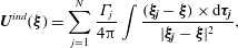 $$\begin{eqnarray}\displaystyle \boldsymbol{U}^{ind}(\unicode[STIX]{x1D743})=\mathop{\sum }_{j=1}^{N}\frac{\unicode[STIX]{x1D6E4}_{j}}{4\unicode[STIX]{x03C0}}\int \frac{(\unicode[STIX]{x1D743}_{\boldsymbol{j}}-\unicode[STIX]{x1D743})\times \text{d}\unicode[STIX]{x1D749}_{\boldsymbol{j}}}{|\unicode[STIX]{x1D743}_{\boldsymbol{j}}-\unicode[STIX]{x1D743}|^{2}}, & & \displaystyle\end{eqnarray}$$
where the integrals cover each vortex filament defined by its circulation
 $\unicode[STIX]{x1D6E4}_{j}$
, its position vector
 $\unicode[STIX]{x1D743}_{\boldsymbol{j}}$
and its tangent vector
 $\unicode[STIX]{x1D749}_{\boldsymbol{j}}$
.
On the vortex line, the Biot–Savart integral is singular, and the self-induced velocity diverges. To avoid this singularity, one has to assume a small but finite core size
 $a$
. The self-induced motion is then obtained by an integral of the same form but without considering the interval
 $[-\unicode[STIX]{x1D6FF}a,\unicode[STIX]{x1D6FF}a]$
around the singular point. This so-called cutoff method is explained at length in textbooks (see Saffman Reference Saffman1992). The value of
 $\unicode[STIX]{x1D6FF}$
depends on the vortex core model. Here, we shall assume a Gaussian vorticity profile for which
 $\unicode[STIX]{x1D6FF}\approx 0.8736$
.
2.2 Vortex discretization
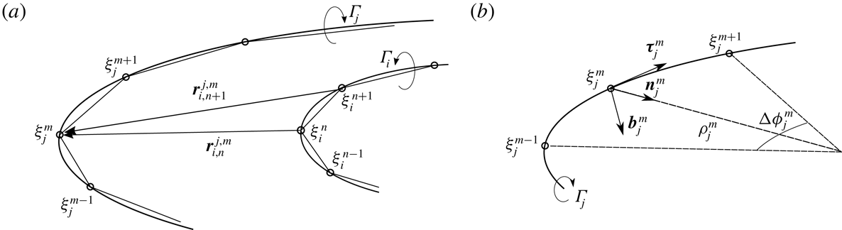
We follow the vortex method approach described for instance in Leishman (Reference Leishman2006). Each vortex filament is discretized in small segments in order to compute the velocity field and follow its displacement (see figure 1 a).
Discretization procedure of the vortex filaments. (a) Discretization in segments of two filaments of circulation
 $\unicode[STIX]{x1D6E4}_{i}$
and
 $\unicode[STIX]{x1D6E4}_{j}$
. (b) Arc of circle formed by three consecutive points of a discretized filament for the computation of the local contribution.
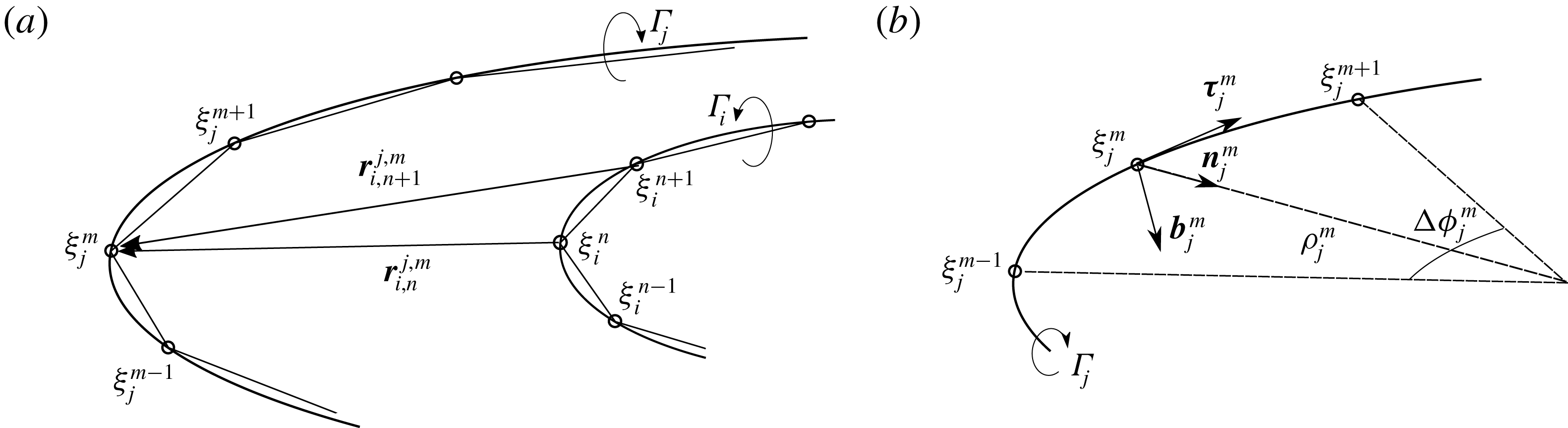
The velocity field induced by a given segment
 $[\unicode[STIX]{x1D743}_{i}^{n},\unicode[STIX]{x1D743}_{i}^{n+1}]$
of the
 $i$
th vortex at a point
 $\unicode[STIX]{x1D743}_{j}^{m}$
can be calculated explicitly as
 $$\begin{eqnarray}\displaystyle \boldsymbol{U}_{i,n}^{seg}(\unicode[STIX]{x1D743}_{j}^{m})=\frac{\unicode[STIX]{x1D6E4}_{i}}{4\unicode[STIX]{x03C0}}\frac{((1-|\boldsymbol{r}_{i,n}^{j,m}|^{2})|\boldsymbol{r}_{i,n}^{j,m}|+(1-|\boldsymbol{r}_{i,n}^{j,m}|^{2})|\boldsymbol{r}_{i,n+1}^{j,m}|)(\boldsymbol{r}_{i,n}^{j,m}\times \boldsymbol{r}_{i,n+1}^{j,m})\boldsymbol{r}_{i,n}^{j,m}\cdot \boldsymbol{r}_{i,n+1}^{j,m}}{((\boldsymbol{r}_{i,n}^{j,m}\cdot \boldsymbol{r}_{i,n+1}^{j,m})^{2}-|\boldsymbol{r}_{i,n}^{j,n}|^{2}|\boldsymbol{r}_{i,n+1}^{j,m}|^{2})|\boldsymbol{r}_{i,n}^{j,m}||\boldsymbol{r}_{i,n+1}^{j,m}|}, & & \displaystyle\end{eqnarray}$$
where
 $\boldsymbol{r}_{i,n}^{j,m}=\unicode[STIX]{x1D743}_{j}^{m}-\unicode[STIX]{x1D743}_{i}^{n}$
. This expression is defined everywhere except at the points
 $\unicode[STIX]{x1D743}_{i}^{n}$
and
 $\unicode[STIX]{x1D743}_{i}^{n+1}$
defining the segment. To determine the contribution to the velocity field at
 $\unicode[STIX]{x1D743}_{j}^{m}$
of the adjacent segments
 $[\unicode[STIX]{x1D743}_{j}^{m},\unicode[STIX]{x1D743}_{j}^{m+1}]$
and
 $[\unicode[STIX]{x1D743}_{j}^{m-1},\unicode[STIX]{x1D743}_{j}^{m}]$
, we replace the two segments by the arc of circle passing through the three points
 $(\unicode[STIX]{x1D743}_{j}^{m-1},\unicode[STIX]{x1D743}_{j}^{m},\unicode[STIX]{x1D743}_{j}^{m+1})$
and use the cutoff formula. We obtain
 $$\begin{eqnarray}\displaystyle \boldsymbol{U}_{j,m}^{loc}=\frac{\unicode[STIX]{x1D6E4}_{j}}{4\unicode[STIX]{x03C0}\unicode[STIX]{x1D70C}_{j}^{m}}\ln \left(\frac{\unicode[STIX]{x0394}\unicode[STIX]{x1D719}_{j}^{m}\unicode[STIX]{x1D70C}_{j}^{m}}{\unicode[STIX]{x1D6FF}a}\right)\boldsymbol{b}_{\boldsymbol{j}}^{\boldsymbol{m}}, & & \displaystyle\end{eqnarray}$$
where
 $\unicode[STIX]{x1D70C}_{j}^{m}$
and
 $\boldsymbol{b}_{j}^{m}$
are the curvature radius and binormal vector at
 $\unicode[STIX]{x1D743}_{j}^{m}$
respectively, and
 $\unicode[STIX]{x0394}\unicode[STIX]{x1D719}_{j}^{m}$
is the angle of the arc of circle
 $(\unicode[STIX]{x1D743}_{j}^{m-1},\unicode[STIX]{x1D743}_{j}^{m+1})$
as illustrated in figure 1(b). The total induced velocity at
 $\unicode[STIX]{x1D743}_{\boldsymbol{j}}^{\boldsymbol{m}}$
is then given by an expression of the form
 $$\begin{eqnarray}\displaystyle \boldsymbol{U}^{ind}(\unicode[STIX]{x1D743}_{j}^{m})=\boldsymbol{U}_{j,m}^{loc}+\mathop{\sum }_{n=1}^{N}\mathop{\sum }_{i=1}^{p_{n}}\boldsymbol{U}_{i,n}^{seg}(\unicode[STIX]{x1D743}_{j}^{m}), & & \displaystyle\end{eqnarray}$$
where
 $p_{n}$
is the number of points discretizing the
 $n$
th vortex, and assuming implicitly that
 $\boldsymbol{U}_{j,m}^{seg}(\unicode[STIX]{x1D743}_{j}^{m})=\boldsymbol{U}_{j,m-1}^{seg}(\unicode[STIX]{x1D743}_{j}^{m})=0$
.
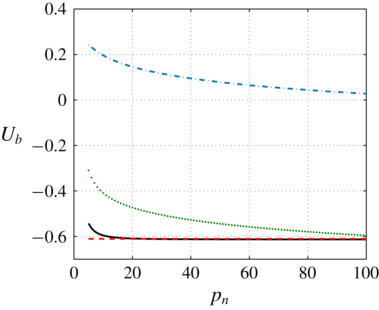
This formula is tested against direct calculation of the cutoff integral in figure 2 for a single helix (see also Gupta & Leishman Reference Gupta and Leishman2005). We observe that a good approximation is obtained as soon as the helix is divided into 25 or more segments by turn when the local contribution is included. When the local contribution is not taken into account, a much larger number of segments by turn of order
 $O(2\unicode[STIX]{x03C0}\unicode[STIX]{x1D70C}/a)$
is needed to obtain a good approximation. In practice, we use
 $p_{n}=30$
in most calculations.
Comparison of the cutoff formula (dashed red line) with the approximate formula (2.5) (solid black line). Binormal component of the induced velocity versus the number
 $p_{n}$
of segments by turn for an helix of circulation
 $\unicode[STIX]{x1D6E4}=1$
, pitch
 $h=1$
, radius
 $R=1$
and core size
 $a=0.05$
. The two contributions
 $\boldsymbol{U}^{loc}$
and
 $\boldsymbol{U}^{seg}$
are also indicated by the dash-dot and dotted lines, respectively.
2.3 Vortex ring and helical vortex
A vortex ring and a helical vortex are examples of vortex structures that move in space at a constant speed without deformation. For these particular vortices, there exist a unique moving frame where all the vortex elements are steady. For the ring, this frame is translating along the ring axis. For the helix, it is both translating and rotating along the helix axis.
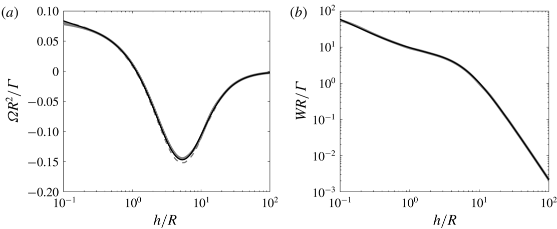
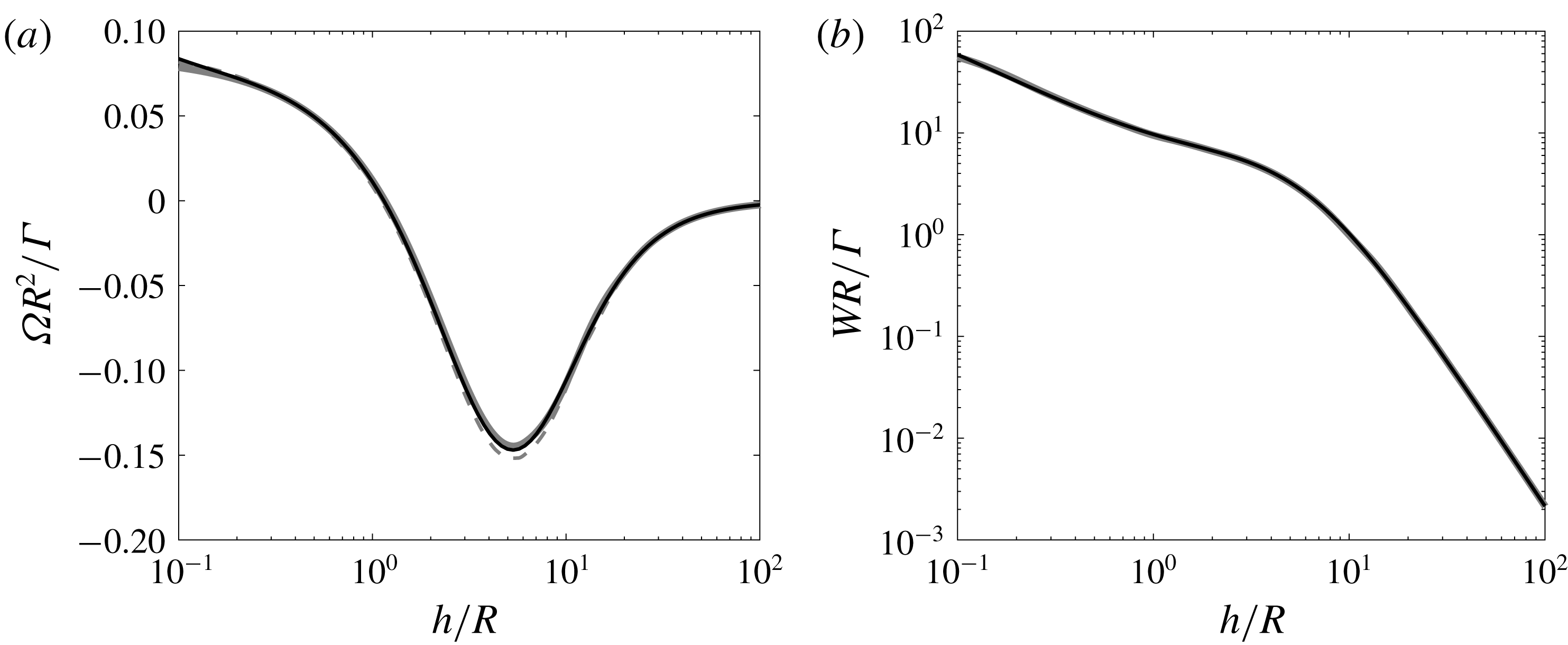
The variation of the rotation rate and axial speed of a right-handed helix with respect to the pitch is given in figure 3 for a typical vortex core size. As already noticed by Velasco Fuentes (Reference Velasco Fuentes2018), it is interesting to see that the rotation changes sign as the pitch varies. For a left-handed helix, the rotation rate is the same but the axial speed is opposite. In figure 3, our numerical results are compared to theoretical approximations based on Hardin (Reference Hardin1982) expressions. The dashed grey curves are obtained by taking the mean value of Hardin expression at
 $R-a$
and
 $R+a$
as it was done by Velasco Fuentes (Reference Velasco Fuentes2018). The solid dashed line is the same expression corrected by a
 $1/4$
term associated with local curvature (Ricca Reference Ricca1994; Kuibin & Okulov Reference Kuibin and Okulov1998; Boersma & Wood Reference Boersma and Wood1999). This correction term permits us to take into account the deformation of the vortex core induced by curvature. For completeness, we provide these expressions of
 $\unicode[STIX]{x1D6FA}$
and
 $W$
in appendix A. In these theoretical works, a Rankine vortex model (uniform vorticity in the core) is used, while we use a Gaussian vorticity profile. We have thus applied the correction factor
 $a_{Rankine}\approx 1.36\,a_{Gaussian}$
to the core size to account for the different vortex models (Widnall Reference Widnall1972; Saffman Reference Saffman1992). As it can be seen on this figure, the agreement between the numerical results and Velasco Fuentes (Reference Velasco Fuentes2018) is good and almost perfect for both
 $\unicode[STIX]{x1D6FA}$
and
 $W$
when the correction term is included. This comparison is a strong validation of our numerical approach.
Non-dimensionalized rotation rate
 $\unicode[STIX]{x1D6FA}R^{2}/\unicode[STIX]{x1D6E4}$
(a) and axial speed
 $WR/\unicode[STIX]{x1D6E4}$
(b) of a right-handed helix of circulation
 $\unicode[STIX]{x1D6E4}$
, radius
 $R$
, pitch
 $h$
and core size
 $a$
as a function of
 $h/R$
for
 $a/R=0.03$
. The solid black curves correspond to the numerical results obtained in this work. The solid grey curves correspond to the theoretical expressions (A 1a,b
), the dashed grey curves correspond to the results obtained by Velasco Fuentes (Reference Velasco Fuentes2018), that is the same expressions without the
 $1/4$
terms. Both theoretical results are for an equivalent Rankine vortex of core size
 $a/R=0.0408$
.
For both rings and helices, there exist infinitely many other moving frames where the vortex structure is steady. The displacement associated with this frame just has to remain tangent to the structure. The condition of steadiness for the frame velocity
 $\boldsymbol{V}_{F}$
can then be written as
 $$\begin{eqnarray}\displaystyle (\boldsymbol{V}_{F}(\unicode[STIX]{x1D743}_{j}^{m})+\boldsymbol{U}^{ind}(\unicode[STIX]{x1D743}_{j}^{m}))\times \unicode[STIX]{x1D749}_{j}^{m}=\mathbf{0}. & & \displaystyle\end{eqnarray}$$
In this frame, the vortex elements are moving along the vortex structure. For a ring, any rotation around the ring axis can for instance be added. For an helix of pitch
 $h$
, any rotation and translation along the helix axis can also be added if the rotation rate
 $\unicode[STIX]{x1D6FA}_{a}$
and axial speed
 $W_{a}$
of this additional movement satisfy
 $$\begin{eqnarray}\displaystyle W_{a}/\unicode[STIX]{x1D6FA}_{a}=\pm h/2\unicode[STIX]{x03C0}, & & \displaystyle\end{eqnarray}$$
where the sign is
 $+$
for right-handed helices, and
 $-$
for left-handed helices.
An helical braid composed of
 $N$
identical vortices of same axis, separated with each other by an azimuthal angle
 $2\unicode[STIX]{x03C0}/N$
also forms a steady solution in an adequate frame. When
 $N\neq 1$
, a straight hub vortex placed on the central axis can be added without introducing any deformation on the helices. This is not possible when
 $N=1$
. The external helix indeed generates an horizontal velocity on the axis that induces a radial displacement of any straight structure place at this position. In that case, we expect the hub vortex to deform and to move out from the rotation axis. Our objective is to describe such a structure, as well as the structures composed of
 $N$
vortex pairs with root vortices not on the rotation axis. We shall see that there still exist steady solutions in those cases.
2.4 Non-interacting helical pairs
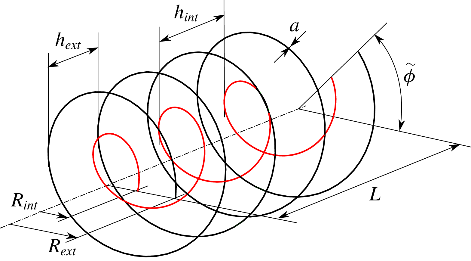
In order to understand the parameters defining the solutions, it is useful to consider first a simple configuration composed of two co-axial helices of opposite circulation and same core size
 $a$
. The internal and external helices are defined by their radii
 $R_{int}$
and
 $R_{ext}$
and pitches
 $h_{int}$
and
 $h_{ext}$
, as illustrated in figure 4. They also depend on their relative orientation characterized by a parameter
 $\unicode[STIX]{x1D705}$
, which is
 $+1$
if both helices have the same orientation, and
 $-1$
if they have opposite orientations.
Configuration of two undeformed co-axial helical vortices. Here both helices have the same orientation:
 $\unicode[STIX]{x1D705}=1$
.
If
 $\unicode[STIX]{x1D705}=-1$
or if
 $h_{ext}\neq h_{int}$
, this pair of vortices is no longer helically invariant. However, it exhibits a certain spatial periodicity. The periodicity is in the sense that there exists an axial distance
 $L>0$
and an angle
 $0\leqslant \tilde{\unicode[STIX]{x1D719}}<2\unicode[STIX]{x03C0}$
such that the radial locations of each vortex are invariant by the double operation of translation by
 $L$
and rotation by
 $\tilde{\unicode[STIX]{x1D719}}$
(see figure 4). The parameters
 $L$
and
 $\tilde{\unicode[STIX]{x1D719}}$
are given by
 $$\begin{eqnarray}\displaystyle & \displaystyle \frac{1}{L}=\left|\frac{1}{h_{int}}-\frac{\unicode[STIX]{x1D705}}{h_{ext}}\right|, & \displaystyle\end{eqnarray}$$
 $$\begin{eqnarray}\displaystyle & \displaystyle \tilde{\unicode[STIX]{x1D719}}=2\unicode[STIX]{x03C0}\left[\frac{L}{\min (h_{int},h_{ext})}-E\left(\frac{L}{\min (h_{int},h_{ext})}\right)\right], & \displaystyle\end{eqnarray}$$
 $E(x)$
denotes the integer part of
 $x$
. When
 $\unicode[STIX]{x1D705}=-1$
,
 $L$
is smaller than
 $h_{ext}$
and
 $h_{int}$
; both helices have performed less than a complete rotation in one axial period
 $L$
. When
 $\unicode[STIX]{x1D705}=1$
,
 $L$
is always larger than the smaller pitch; the helix with the smaller pitch has then performed more than a complete rotation in a period. The other helix has performed just one complete revolution less.
When
 $h_{ext}\neq h_{int}$
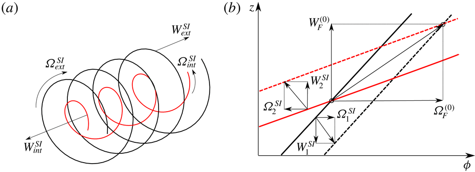
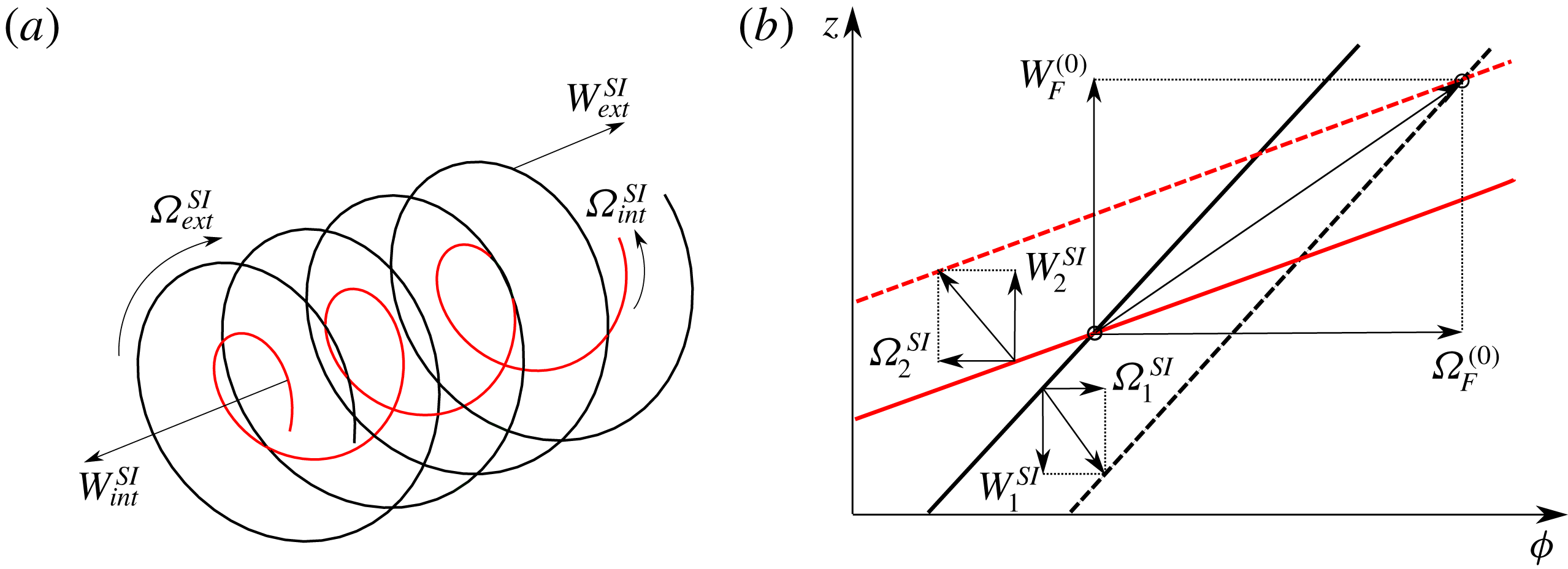
, the undeformed helical pair corresponds to a steady solution only if the mutual induction of one helix on the other is negligible. This occurs when the core size becomes sufficiently small. In this limit, the locally induced velocity is the dominant contribution to the induced velocity which then becomes constant and oriented along the local binormal vector. Each helix then behaves as if the other helix was not present. A priori, they rotate and translate at different speeds. But, owing to the possibility to add any displacement along the helical line, it is possible to find a frame where both helical structures become steady. The frame selection is graphically explained in figure 5(b). In that figure, we plot each helix in the
 $(\unicode[STIX]{x1D719},z)$
plane at
 $t=0$
(solid lines) and
 $t=1$
(dashed lines) using two different colours. Each helix corresponds to a straight line with a slope equal to the helix pitch. The self-induced velocity of each helix, together with their decomposition in the axial and azimuthal directions, is also indicated. Any vector that connects any two points from the lines at the two distinct times provides a possible frame velocity vector that keeps the considered helix steady. The vector that keeps both helices steady is the one that connects the crossing points associated with each instant. Such a vector exists as soon as the helix lines are not parallel in the
 $(\unicode[STIX]{x1D719},z)$
plane, that is if
 $h_{ext}\neq h_{int}$
or
 $\unicode[STIX]{x1D705}=-1$
.
(a) Self-induced velocities of a pair of coaxial vortices when the mutual induction is negligible. (b) Schematic diagram showing how the moving frame velocities
 $\unicode[STIX]{x1D6FA}_{F}^{(0)}$
and
 $W_{F}^{(0)}$
are obtained. Solid and dashed lines represent the two helices at
 $t=0$
and
 $t=1$
respectively. The frame velocity is given by the vector connecting the crossing points of solid lines with dashed lines. The axial and azimuthal components of this vector provides
 $W_{F}^{(0)}$
and
 $\unicode[STIX]{x1D6FA}_{F}^{(0)}$
respectively.
The angular velocity
 $\unicode[STIX]{x1D6FA}_{F}^{(0)}$
and axial velocity
 $W_{F}^{(0)}$
of the frame are given from the self-induced velocity of each helix by
 $$\begin{eqnarray}\displaystyle & \displaystyle \unicode[STIX]{x1D6FA}_{F}^{(0)}=\frac{2\unicode[STIX]{x03C0}(W_{int}^{SI}-W_{ext}^{SI})+(\unicode[STIX]{x1D6FA}_{ext}^{SI}h_{ext}-\unicode[STIX]{x1D6FA}_{int}^{SI}\unicode[STIX]{x1D705}h_{int})}{h_{ext}-\unicode[STIX]{x1D705}h_{int}}, & \displaystyle\end{eqnarray}$$
 $$\begin{eqnarray}\displaystyle & \displaystyle W_{F}^{(0)}=W_{ext}^{SI}+\frac{h_{ext}}{2\unicode[STIX]{x03C0}}(\unicode[STIX]{x1D6FA}_{F}^{(0)}-\unicode[STIX]{x1D6FA}_{ext}^{SI}). & \displaystyle\end{eqnarray}$$
 $$\begin{eqnarray}\displaystyle W_{F}^{(0)}=W_{int}^{SI}+\frac{\unicode[STIX]{x1D705}h_{int}}{2\unicode[STIX]{x03C0}}(\unicode[STIX]{x1D6FA}_{F}^{(0)}-\unicode[STIX]{x1D6FA}_{int}^{SI}), & & \displaystyle\end{eqnarray}$$
that guarantees that (2.7) is also satisfied by the internal vortex.
Without restriction, we can assume the external helix to be right-handed with a positive circulation
 $\unicode[STIX]{x1D6E4}$
. The internal helix has then a negative circulation
 $-\unicode[STIX]{x1D6E4}$
. It is right-handed if
 $\unicode[STIX]{x1D705}=1$
, left-handed if
 $\unicode[STIX]{x1D705}=-1$
.
2.5 Parameters defining the deformed helical structures
The two-helix structure obtained above is no longer a solution if the two helices interact. Indeed, the velocity field of one helix on the other contains a radial component that moves the structure radially. Each helix is therefore expected to be deformed by the field induced by the other helices. Being inspired by the non-interacting solutions, we shall search for steady solutions that still exhibit a spatial periodicity. We consider solutions composed of
 $N$
pairs of counter-rotating vortices (the external vortex having a positive circulation
 $\unicode[STIX]{x1D6E4}$
, the internal a negative circulation
 $-\unicode[STIX]{x1D6E4}$
), with a
 $2\unicode[STIX]{x03C0}/N$
azimuthal symmetry. By construction, we then assume that the solutions are invariant by the transform
 $\unicode[STIX]{x1D719}\rightarrow \unicode[STIX]{x1D719}+2\unicode[STIX]{x03C0}/N$
. We also assume that there exist an axial distance
 $L>0$
and an angle
 $\tilde{\unicode[STIX]{x1D719}}$
satisfying
 $0\leqslant \tilde{\unicode[STIX]{x1D719}}<2\unicode[STIX]{x03C0}/N$
, such that the solutions are invariant by the double operation
 $z\rightarrow z+L$
and
 $\unicode[STIX]{x1D719}\rightarrow \unicode[STIX]{x1D719}+\tilde{\unicode[STIX]{x1D719}}$
. We do not want the solution to repeat several times in a spatial period, so we further assume that there is a single location in an axial period
 $L$
where internal and external vortices are at the same azimuth. We shall choose this particular azimuth to define, from their radial positions, the radii
 $R_{int}$
and
 $R_{ext}$
of the internal and external vortex (
 $R_{int}<R_{ext}$
). We also define the mean pitch
 $h_{int}$
and
 $h_{ext}$
for each vortex from the azimuthal angle covered in an axial period. For the external vortex, if this angle is
 $\unicode[STIX]{x1D719}_{ext}$
, we have
 $h_{ext}=2\unicode[STIX]{x03C0}L/\unicode[STIX]{x1D719}_{ext}$
. If we add the vortex core size
 $a$
that we assume identical and constant for all the vortices, we obtain five spatial length scales from which we can form four independent non-dimensional parameters:
 $$\begin{eqnarray}\displaystyle R^{\ast }=\frac{R_{int}}{R_{ext}},\quad h^{\ast }=\frac{h_{ext}}{R_{ext}},\quad \unicode[STIX]{x1D6FC}=\frac{h_{int}}{h_{ext}},\quad \unicode[STIX]{x1D700}=\frac{a}{R_{ext}}. & & \displaystyle\end{eqnarray}$$
To these four real positive parameters, we should add the number
 $N$
of vortex pairs and the index
 $\unicode[STIX]{x1D705}=\pm 1$
that defines the relative orientation of internal and external vortices. In most cases, we shall keep
 $\unicode[STIX]{x1D705}=1$
and
 $N=1$
. The parameter
 $R^{\ast }$
will be varied between 0 and 0.75,
 $h^{\ast }$
between 0.1 and 2,
 $\unicode[STIX]{x1D6FC}$
between 0.5 and 2. The parameter
 $\unicode[STIX]{x1D700}$
will always be considered small, and typically equal to 0.03. Even for this small value of
 $\unicode[STIX]{x1D700}$
, finite core size effects can become important if
 $h$
and
 $\unicode[STIX]{x1D6FC}$
are too small. This provides a limitation on the values of the parameters that we can consider. Here, only the extreme cases (
 $h\approx 0.1$
and
 $\unicode[STIX]{x1D6FC}\approx 0.5$
) are expected to give rise to consequent finite core size effects.
In the paper, the vortex core size is also assumed to be constant. This approximation is discussed in § 4.
Note that both the normalized period
 $L/R_{ext}$
and the angle
 $\tilde{\unicode[STIX]{x1D719}}$
can be obtained from the above geometrical parameters:
 $$\begin{eqnarray}\displaystyle \frac{L}{R_{ext}}=\frac{h^{\ast }}{N|1/\unicode[STIX]{x1D6FC}-\unicode[STIX]{x1D705}|},\quad \tilde{\unicode[STIX]{x1D719}}=\frac{2\unicode[STIX]{x03C0}}{N}\left[\frac{1}{|1/\unicode[STIX]{x1D6FC}-\unicode[STIX]{x1D705}|}-E\left(\frac{1}{|1/\unicode[STIX]{x1D6FC}-\unicode[STIX]{x1D705}|}\right)\right]. & & \displaystyle\end{eqnarray}$$
Each solution is associated with a moving frame where the solution is steady. From the angular velocity
 $\unicode[STIX]{x1D6FA}_{F}$
and the axial velocity
 $W_{F}$
of the frame, we can construct two other dimensionless parameters using the external radius
 $R_{ext}$
and the circulation
 $\unicode[STIX]{x1D6E4}$
of the vortices:
 $$\begin{eqnarray}\displaystyle \unicode[STIX]{x1D6FA}=\frac{R_{ext}^{2}\unicode[STIX]{x1D6FA}_{F}}{N\unicode[STIX]{x1D6E4}},\quad W=\frac{R_{ext}W_{F}}{N\unicode[STIX]{x1D6E4}}. & & \displaystyle\end{eqnarray}$$
These two parameters characterizing the frame velocity are functions of the six geometrical parameters
 $R^{\ast }$
,
 $h^{\ast }$
,
 $\unicode[STIX]{x1D6FC}$
,
 $\unicode[STIX]{x1D700}$
,
 $N$
and
 $\unicode[STIX]{x1D705}$
.
3 Deformed helical vortex pairs
In this section, we describe the deformed helical structures as the geometrical parameters vary. After having introduced an approximated solution, we successively study the geometrical characteristics, the frame velocity and the induced velocity.
3.1 First-order approximation
As already mentioned above, as soon as the mutual induction of one helix on the others is taken into account, the vortex structure does not remain helical. For a given vortex parametrized by its radial position
 $r(z)$
and angular position
 $\unicode[STIX]{x1D719}(z)$
as a function of the
 $z$
coordinate, the condition of steadiness (2.6) reduces to
 $$\begin{eqnarray}\displaystyle \frac{\text{d}r}{\text{d}z}=\frac{V_{r}^{ind}}{V_{z}^{ind}-W_{F}},\quad \frac{\text{d}\unicode[STIX]{x1D719}}{\text{d}z}=\frac{\unicode[STIX]{x1D6FA}^{ind}-\unicode[STIX]{x1D6FA}_{F}}{V_{z}^{ind}-W_{F}}. & & \displaystyle\end{eqnarray}$$
Each induced velocity component is composed of two contributions, a self-induced contribution
 $V^{SI}$
and a contribution induced by the other vortices
 $V^{MI}$
. The radial self-induced velocity of an helix being null, we clearly see from the first equation that the radial deformation will be associated with the mutual induction, and more precisely with the radial component
 $V_{r}^{MI}$
of the mutually induced velocity.
A first-order correction to the undeformed solution can be obtained by solving these two equations assuming that the velocity fields on the right-hand side are evaluated at the undeformed location:
 $$\begin{eqnarray}\displaystyle & \displaystyle \frac{\text{d}r^{(1)}}{\text{d}z}=\frac{V_{r}^{MI}(r_{0},\unicode[STIX]{x1D719}_{0}(z),z)}{V_{z}^{MI}(r_{0},\unicode[STIX]{x1D719}_{0}(z),z)+V_{z}^{SI}-W_{F}^{(1)}}, & \displaystyle\end{eqnarray}$$
 $$\begin{eqnarray}\displaystyle & \displaystyle \frac{\text{d}\unicode[STIX]{x1D719}^{(1)}}{\text{d}z}=\frac{\unicode[STIX]{x1D6FA}^{MI}(r_{0},\unicode[STIX]{x1D719}_{0}(z),z)+\unicode[STIX]{x1D6FA}^{SI}-\unicode[STIX]{x1D6FA}_{F}^{(1)}}{V_{z}^{MI}(r_{0},\unicode[STIX]{x1D719}_{0}(z),z)+V_{z}^{SI}-W_{F}^{(1)}}. & \displaystyle\end{eqnarray}$$
 $\unicode[STIX]{x1D6FA}_{F}^{(1)}$
and
 $W_{F}^{(1)}$
are obtained by using the definition of
 $L$
for the internal and external vortices:
 $$\begin{eqnarray}\displaystyle & \displaystyle \unicode[STIX]{x1D719}_{int}^{(1)}(L)-\unicode[STIX]{x1D719}_{int}^{(1)}(0)=\frac{2\unicode[STIX]{x03C0}L}{h_{int}}=\int _{0}^{L}\frac{\unicode[STIX]{x1D6FA}_{int}^{MI}(r_{int}^{(0)},\unicode[STIX]{x1D719}_{int}^{(0)}(z),z)+\unicode[STIX]{x1D6FA}_{int}^{SI}-\unicode[STIX]{x1D6FA}_{F}^{(1)}}{V_{z,int}^{MI}(r_{int}^{(0)},\unicode[STIX]{x1D719}_{int}^{(0)}(z),z)+V_{z,int}^{SI}-W_{F}^{(1)}}\,\text{d}z, & \displaystyle\end{eqnarray}$$
 $$\begin{eqnarray}\displaystyle & \displaystyle \unicode[STIX]{x1D719}_{ext}^{(1)}(L)-\unicode[STIX]{x1D719}_{ext}^{(1)}(0)=\frac{2\unicode[STIX]{x03C0}L}{h_{ext}}=\int _{0}^{L}\frac{\unicode[STIX]{x1D6FA}_{ext}^{MI}(r_{ext}^{(0)},\unicode[STIX]{x1D719}_{ext}^{(0)}(z),z)+\unicode[STIX]{x1D6FA}_{ext}^{SI}-\unicode[STIX]{x1D6FA}_{F}^{(1)}}{V_{z,ext}^{MI}(r_{ext}^{(0)},\unicode[STIX]{x1D719}_{ext}^{(0)}(z),z)+V_{z,ext}^{SI}-W_{F}^{(1)}}\,\text{d}z. & \displaystyle\end{eqnarray}$$
Radial position of the internal and external vortices for a single counter-rotating helical pair for (a)
 $R^{\ast }=0.5$
,
 $\unicode[STIX]{x1D705}=1$
,
 $h^{\ast }=1$
,
 $\unicode[STIX]{x1D6FC}=0.9$
and
 $\unicode[STIX]{x1D700}=0.03$
(b)
 $R^{\ast }=0.5$
,
 $\unicode[STIX]{x1D705}=1$
,
 $h^{\ast }=1$
,
 $\unicode[STIX]{x1D6FC}=1.4$
and
 $\unicode[STIX]{x1D700}=0.03$
. Solid line: numerical solution. Dashed line: first-order approximation.
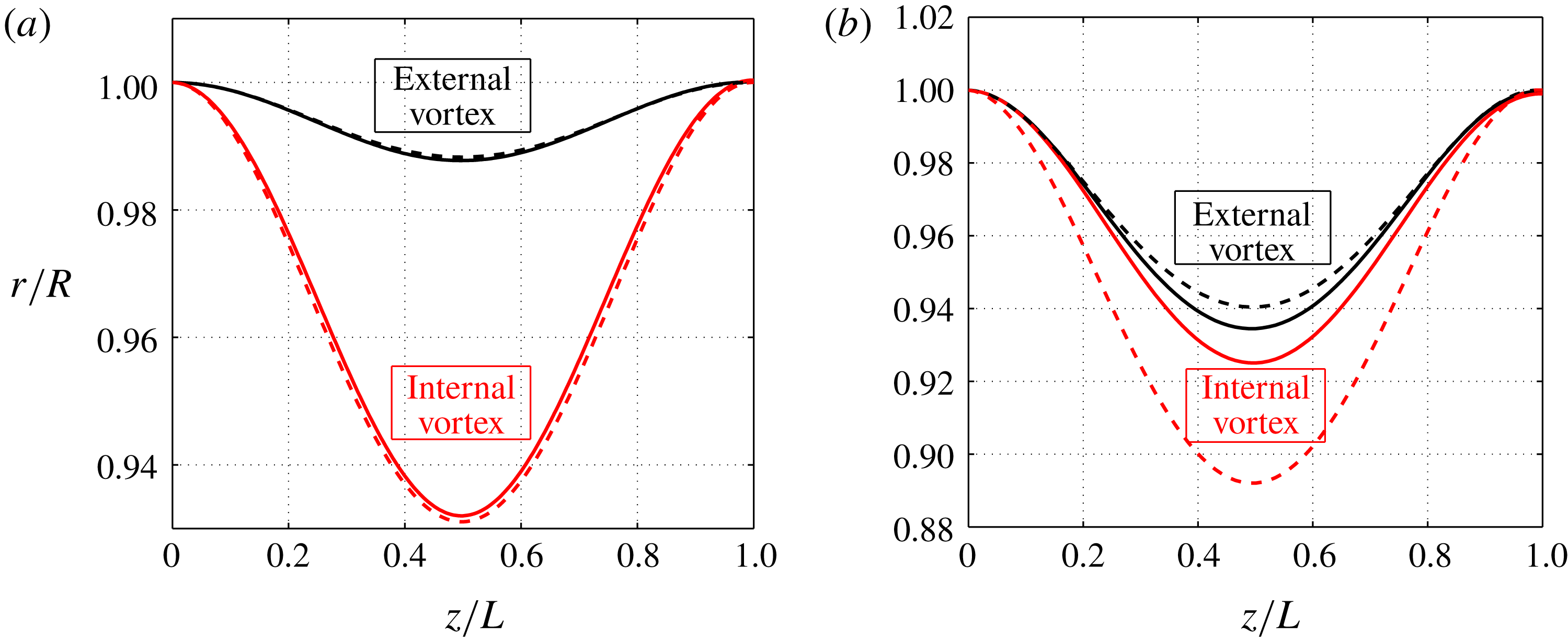
This simple first-order approximation for the helix deformation is compared to numerical results for two typical examples in figure 6. We clearly see that the agreement strongly depends on the pitch ratio
 $\unicode[STIX]{x1D6FC}$
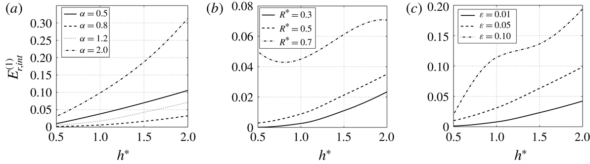
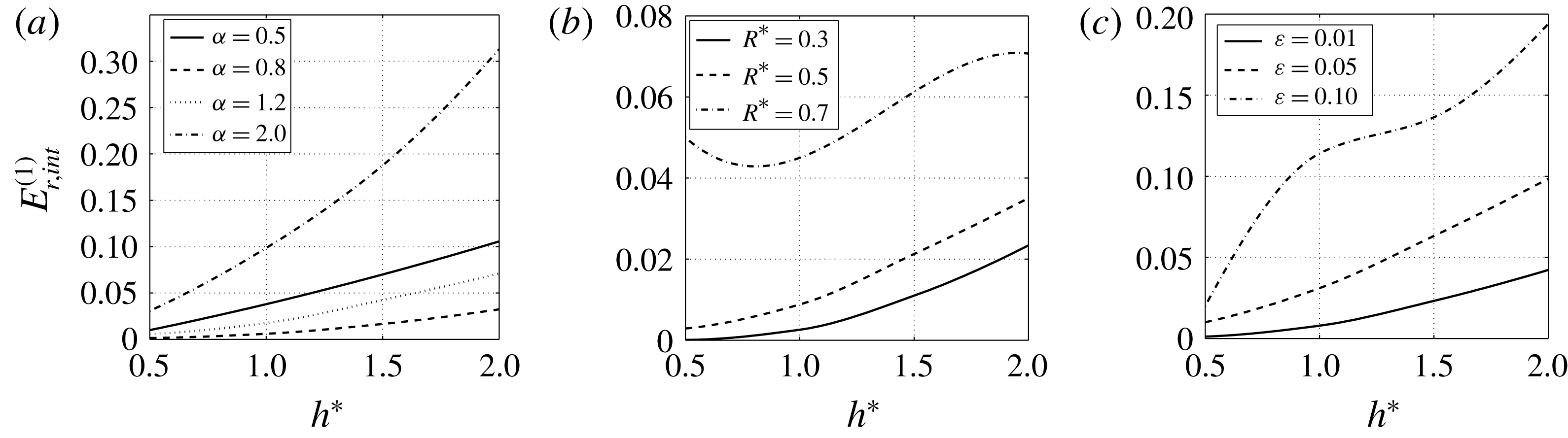
. This approximation tends to underestimate the deformation of the external vortex but to overestimate that of the internal vortex. The error is always larger for the internal vortex. The maximum error can then be quantified using
 $$\begin{eqnarray}\displaystyle E_{r,int}^{(1)}=\frac{\max (|r_{int}-r_{int}^{(1)}|)}{R_{int}}, & & \displaystyle\end{eqnarray}$$
which measures the maximum deviation between numerical and first-order solutions. This quantity is plotted in figure 7 as a function of
 $h^{\ast }$
for
 $N=\unicode[STIX]{x1D705}=1$
and various
 $\unicode[STIX]{x1D6FC}$
,
 $R^{\ast }$
and
 $\unicode[STIX]{x1D700}$
. This figure shows that, except for very large
 $R^{\ast }$
(
 $R^{\ast }=0.7$
), the error increases with
 $h^{\ast }$
. The error also increases with
 $\unicode[STIX]{x1D700}$
,
 $R^{\ast }$
and with the distance of
 $\unicode[STIX]{x1D6FC}$
to 1. It becomes particularly large (larger than 30 %) for large
 $\unicode[STIX]{x1D6FC}$
and large
 $h^{\ast }$
. Note however that the error remains small for
 $\unicode[STIX]{x1D6FC}\approx 1$
, small
 $R^{\ast }$
and small
 $\unicode[STIX]{x1D700}$
.
First-order approximation error
 $E_{r,int}^{(1)}$
for a single vortex pair (
 $N=\unicode[STIX]{x1D705}=1$
). (a):
 $R^{\ast }=0.5$
and
 $\unicode[STIX]{x1D700}=0.03$
; (b):
 $\unicode[STIX]{x1D6FC}=1.2$
and
 $\unicode[STIX]{x1D700}=0.03$
; (c):
 $R^{\ast }=0.5$
and
 $\unicode[STIX]{x1D6FC}=1.2$
.
3.2 Characterization of the helix deformation
The first-order approximation clearly demonstrates that the radial deformation increases when the radial velocity induced by the other vortices grows. This occurs when internal and external vortices get closer to each other, that is when
 $R^{\ast }$
increases. This is illustrated in figure 8 where a perspective view of a single pair is shown for different values of
 $R^{\ast }$
, the other parameters being fixed.
Representation of the deformed vortex structure for
 $N=1$
,
 $\unicode[STIX]{x1D705}=1$
,
 $h^{\ast }=2$
,
 $\unicode[STIX]{x1D6FC}=1.5$
,
 $\unicode[STIX]{x1D700}=0.06$
and different values of
 $R^{\ast }$
.

In order to quantify the level of deformation, we introduce two quantities
 $$\begin{eqnarray}\displaystyle \unicode[STIX]{x0394}r_{max}^{int}=\frac{\max (|r_{int}-R_{int}|)}{R_{int}},\quad \unicode[STIX]{x0394}r_{max}^{ext}=\frac{\max (|r_{ext}-R_{ext}|)}{R_{ext}} & & \displaystyle\end{eqnarray}$$
that measure the maximum displacement of the internal and external vortices. The growth of
 $\unicode[STIX]{x0394}r_{max}^{int}$
and
 $\unicode[STIX]{x0394}r_{max}^{ext}$
with respect to
 $R^{\ast }$
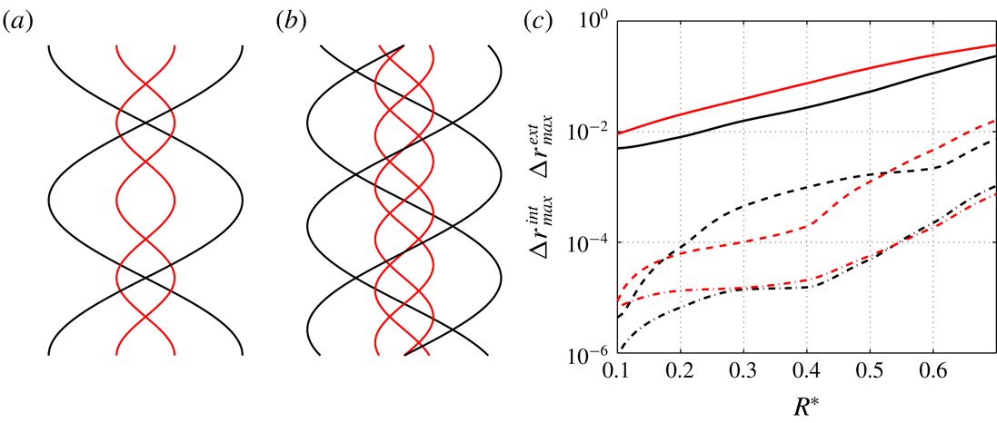
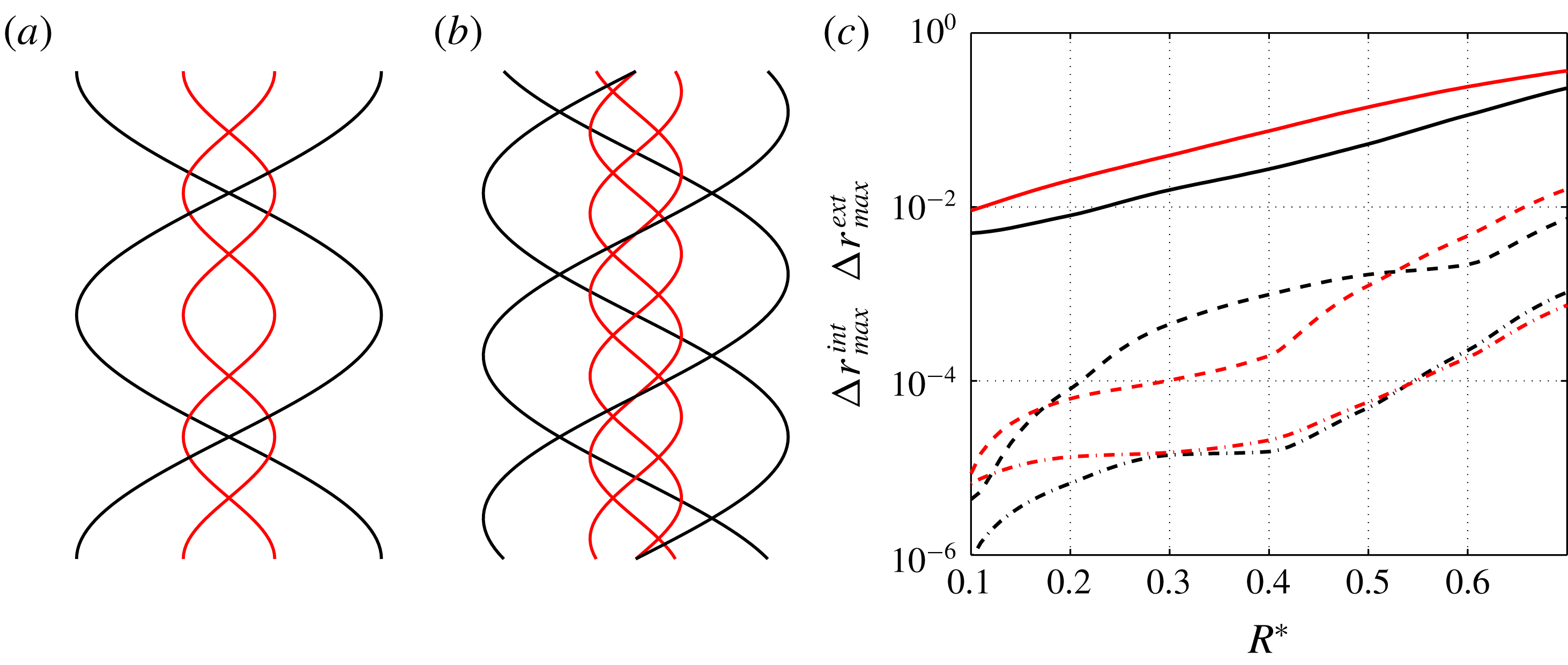
is quantified in figure 9(c). The effect of the number of vortices is clearly visible. The vortex deformation strongly decreases with
 $N$
. For
 $R^{\ast }=0.7$
, the fluctuation of the internal vortex reaches 30 % for a single vortex pair while it is less than 0.1 % for three vortex pairs. Note that when
 $R^{\ast }$
goes to zero, the deformation of the external vortex vanishes whatever
 $N$
. When
 $N\neq 1$
, this is the same for the internal vortex. In that case, we recover the Joukowski’s model with a straight vortex hub on the helix axis. For
 $N=1$
, the limit
 $R^{\ast }\rightarrow 0$
is by contrast singular.
Representation of two vortex pairs (a) and three vortex pairs (b) for
 $h^{\ast }=1$
,
 $R^{\ast }=0.4$
,
 $\unicode[STIX]{x1D700}=0.05$
,
 $\unicode[STIX]{x1D6FC}=2$
,
 $\unicode[STIX]{x1D705}=1$
. (c) Maximum deformation
 $\unicode[STIX]{x0394}r_{max}^{int}$
(red) and
 $\unicode[STIX]{x0394}r_{max}^{ext}$
(black) versus
 $R^{\ast }$
for one vortex pair (solid lines), two vortex pairs (dashed lines), three vortex pairs (dash-dot lines).
 $h^{\ast }=1$
,
 $\unicode[STIX]{x1D6FC}=1.5$
,
 $\unicode[STIX]{x1D705}=1$
and
 $\unicode[STIX]{x1D700}=0.05$
.
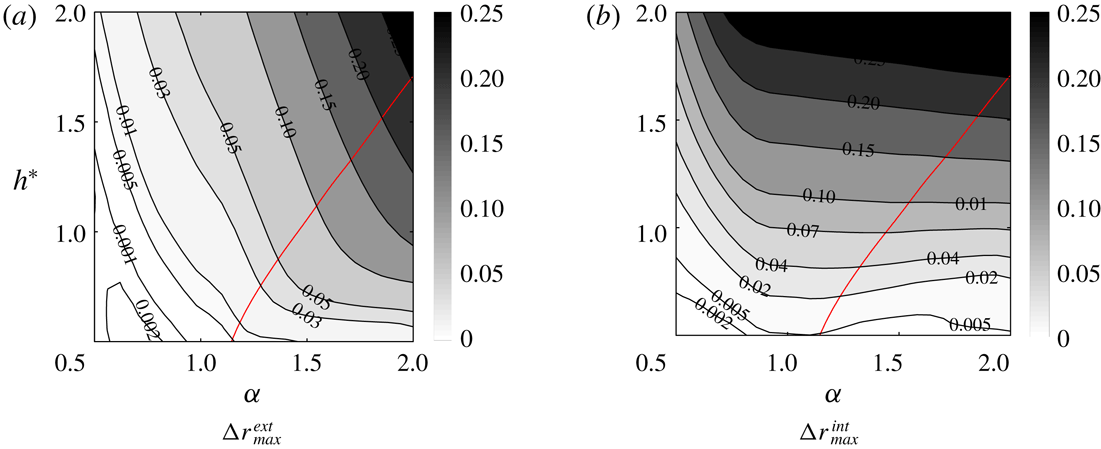
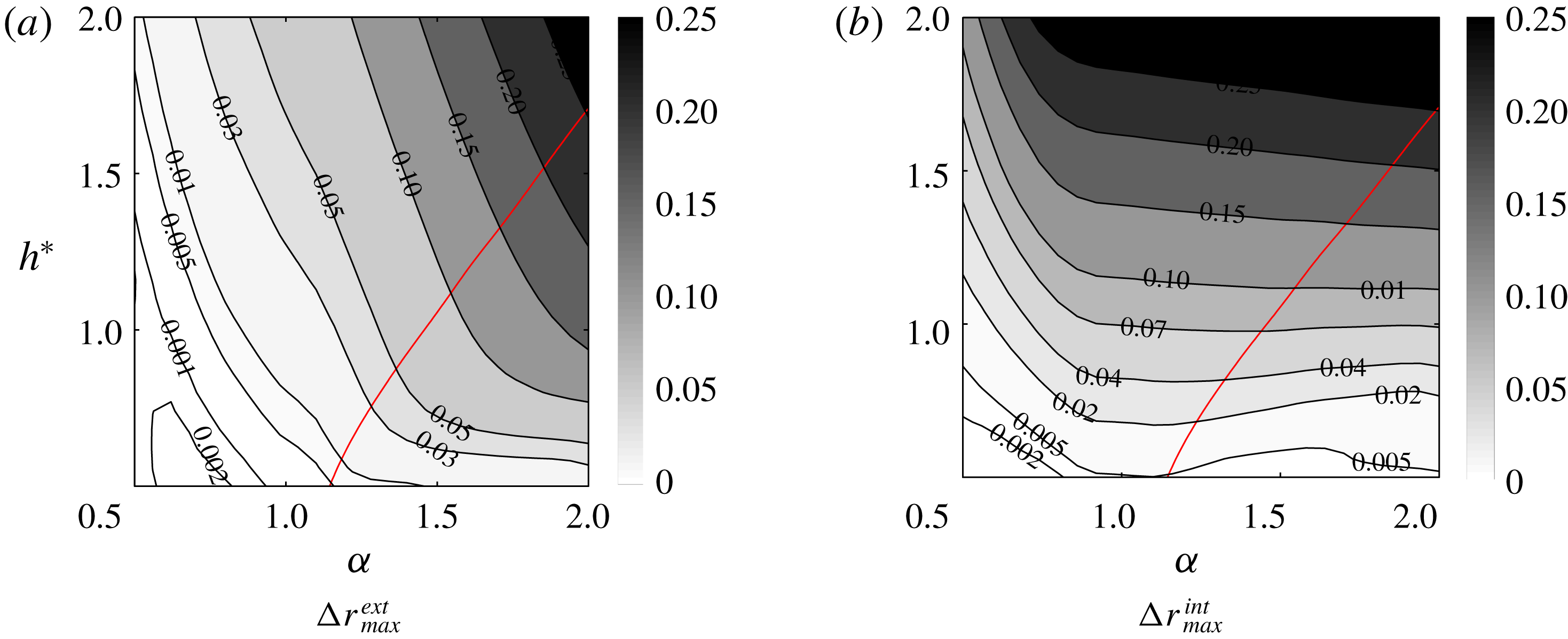
The variations of
 $\unicode[STIX]{x0394}r_{max}^{int}$
and
 $\unicode[STIX]{x0394}r_{max}^{ext}$
with respect to
 $h^{\ast }$
and
 $\unicode[STIX]{x1D6FC}$
are shown in figure 10. The increase of the vortex deformations with
 $h^{\ast }$
is associated with the decrease of the axial component of the induced velocity. Indeed, for large
 $h^{\ast }$
, the vortices become aligned with respect to the
 $z$
axis. They therefore mainly induce a velocity field in the radial and azimuthal directions. The ratio
 $V_{r}/V_{z}$
that defines the slope of the deformation thus gets large, implying large
 $\unicode[STIX]{x0394}r_{max}^{int}$
and
 $\unicode[STIX]{x0394}r_{max}^{ext}$
. In the opposite, when
 $h^{\ast }$
goes to zero,
 $V_{r}/V_{z}$
goes to zero as well: the helical vortices are thus no longer deformed.
Maximum deformation contours in the
 $(\unicode[STIX]{x1D6FC},h)$
plane for
 $R^{\ast }=0.5$
,
 $\unicode[STIX]{x1D700}=0.03$
,
 $\unicode[STIX]{x1D705}=1$
,
 $N=1$
. The thick solid line corresponds to the line
 $\unicode[STIX]{x0394}r_{max}^{int}=\unicode[STIX]{x0394}r_{max}^{ext}$
.
Concerning the effect of
 $\unicode[STIX]{x1D6FC}$
, the increase of the deformation of the external helix with
 $\unicode[STIX]{x1D6FC}$
can be understood by the same argument. It is associated with a decrease of
 $h_{int}$
, and therefore an increase of the ratio
 $V_{r}/V_{z}$
. The variation of
 $\unicode[STIX]{x0394}r_{max}^{int}$
with respect to
 $\unicode[STIX]{x1D6FC}$
is less simple. For
 $h^{\ast }<1$
,
 $\unicode[STIX]{x0394}r_{max}^{int}$
is maximum for
 $\unicode[STIX]{x1D6FC}$
close to 1. This value
 $\unicode[STIX]{x1D6FC}=1$
is special for
 $\unicode[STIX]{x1D705}=1$
because the axial period
 $L$
and the frame axial velocity
 $W_{F}$
become infinite (see (2.12)). It therefore corresponds to a singular limit in our description. However, the radial positions
 $r_{int}$
and
 $r_{ext}$
of internal and external vortices can still be plotted as a function of
 $z/L$
and we obtain a well-defined curve as
 $\unicode[STIX]{x1D6FC}\rightarrow 1$
. Similarly,
 $W_{F}/L$
converges to a non-zero constant as
 $\unicode[STIX]{x1D6FC}\rightarrow 1$
, which means that a finite time
 $T=L/W_{F}$
is needed to advect a perturbation on the period
 $L$
at the velocity
 $W_{F}$
. The singular case
 $\unicode[STIX]{x1D6FC}=1$
could therefore be described in an alternative way by considering the solution in the frame moving at the velocity
 $W_{F}$
. In this frame the solution should correspond to the temporal dynamics of perfect helices with the same
 $R^{\ast }$
,
 $h^{\ast }$
and
 $\unicode[STIX]{x1D700}$
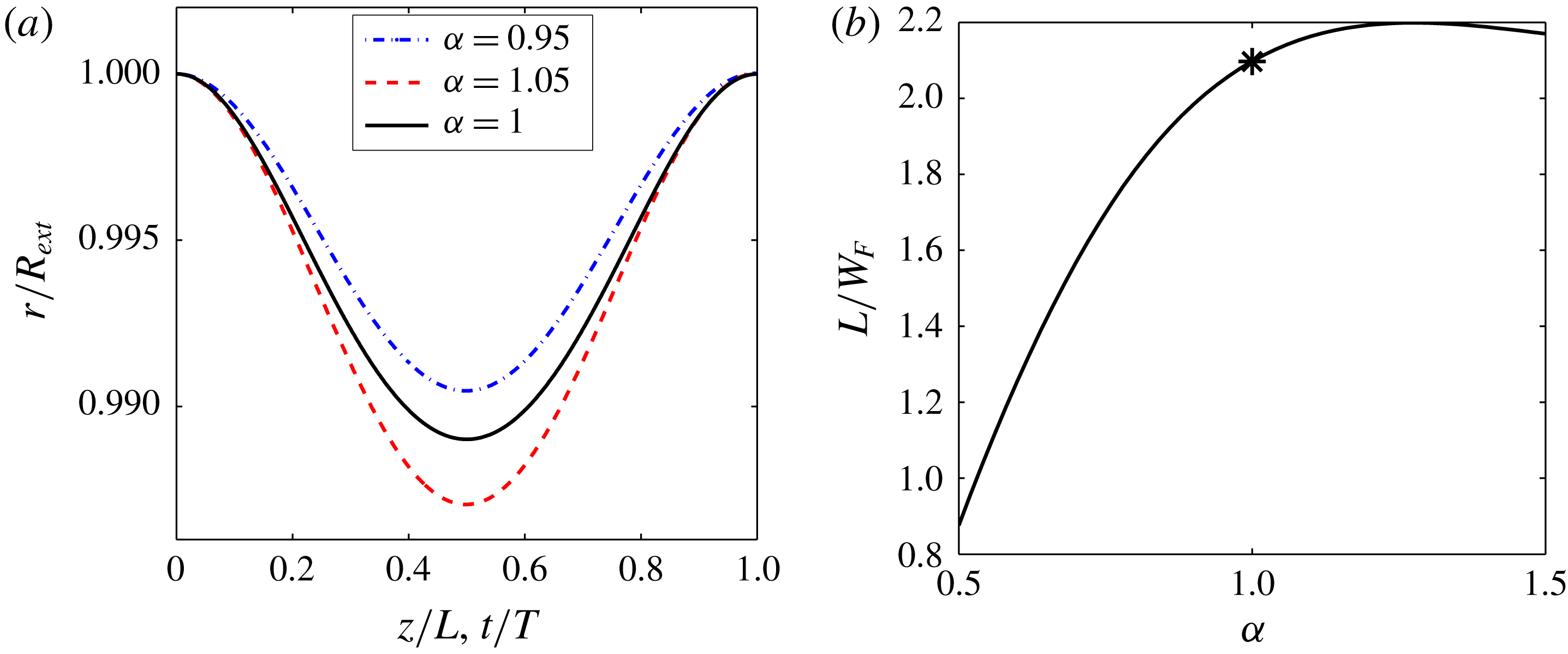
. This is indeed what we have checked in figure 11. In figure 11(a), we show that the variation of
 $r_{ext}$
as a function of
 $z/L$
, for
 $\unicode[STIX]{x1D6FC}$
close to one, is well described by the variation of
 $r_{ext}$
as a function of
 $t/T$
in the temporal problem. We also check in figure 11(b) that
 $L/W_{F}$
converges to the temporal period obtained in the temporal problem as
 $\unicode[STIX]{x1D6FC}\rightarrow 1$
.
Characteristics close to
 $\unicode[STIX]{x1D6FC}=1$
for
 $R^{\ast }=0.5$
,
 $h^{\ast }=1$
,
 $\unicode[STIX]{x1D700}=0.01$
,
 $N=1$
,
 $\unicode[STIX]{x1D705}=1$
. (a) Comparison of the radial positions of the external vortex versus
 $z/L$
for
 $\unicode[STIX]{x1D6FC}=1.05$
and
 $\unicode[STIX]{x1D6FC}=0.95$
with the radial position of the external helix versus
 $t/T$
for
 $\unicode[STIX]{x1D6FC}=1$
. (b) Variation of the characteristic time scale
 $L/W_{F}$
versus
 $\unicode[STIX]{x1D6FC}$
. The symbol represents the period
 $T$
of the temporal evolution of perfect helices for
 $\unicode[STIX]{x1D6FC}=1$
.
3.3 Structure velocities
As explained above (§ 3.1), we can obtain different approximations of the frame velocity
 $\unicode[STIX]{x1D6FA}_{F}$
and
 $W_{F}$
by neglecting the helix deformations and/or the mutual induction. The leading-order approximation (
 $\unicode[STIX]{x1D6FA}_{F}^{(0)}$
,
 $W_{F}^{(0)}$
) neglects both the mutual induction and the deformation. The first-order approximation (
 $\unicode[STIX]{x1D6FA}_{F}^{(1)}$
,
 $W_{F}^{(1)}$
) neglects the vortex deformation but takes into account the mutual induction. This approximation is obtained by solving (3.3a,b
) for
 $\unicode[STIX]{x1D6FA}_{F}^{(1)}$
and
 $W_{F}^{(1)}$
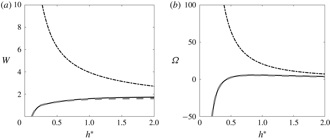
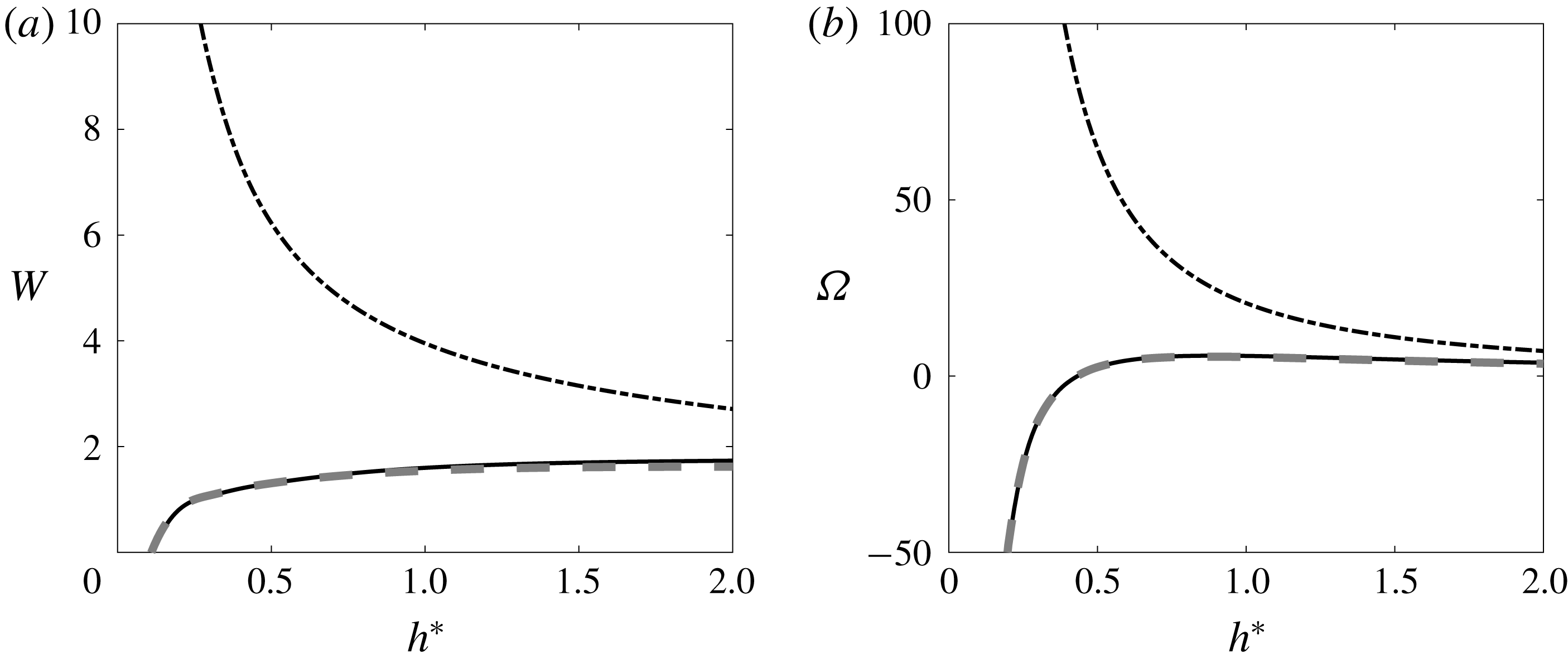
. In figure 12, we have compared both approximations to numerical results for a typical case. We clearly see that the leading-order approximation does not capture the variations of
 $\unicode[STIX]{x1D6FA}_{F}$
and
 $W_{F}$
with
 $h^{\ast }$
, while the first-order approximation follows both qualitatively and quantitatively these variations. By comparing other configurations, we have observed that the first-order approximation provides a good approximation of
 $\unicode[STIX]{x1D6FA}_{F}$
and
 $W_{F}$
as soon as
 $R^{\ast }\leqslant 0.5$
and
 $\unicode[STIX]{x1D700}\leqslant 0.1$
. In practice, these approximations have been used as guess values for the numerical calculation.
Frame velocity versus
 $h^{\ast }$
for
 $R^{\ast }=0.5$
,
 $\unicode[STIX]{x1D700}=0.03$
,
 $\unicode[STIX]{x1D6FC}=1.4$
,
 $\unicode[STIX]{x1D705}=1$
,
 $N=1$
. (a) Angular velocity
 $\unicode[STIX]{x1D6FA}=R_{ext}^{2}\unicode[STIX]{x1D6FA}_{F}/\unicode[STIX]{x1D6E4}$
, (b) axial velocity
 $W=R_{ext}W_{F}/\unicode[STIX]{x1D6E4}$
. Solid line: numerical result. Dashed line: first-order approximation (
 $\unicode[STIX]{x1D6FA}_{F}^{(1)}$
,
 $W_{F}^{(1)}$
). Dash-dotted line: leading-order approximation (
 $\unicode[STIX]{x1D6FA}_{F}^{(0)}$
,
 $W_{F}^{(0)}$
).
The variations of the frame velocities
 $\unicode[STIX]{x1D6FA}$
and
 $W$
with respect to
 $h^{\ast }$
and
 $\unicode[STIX]{x1D6FC}$
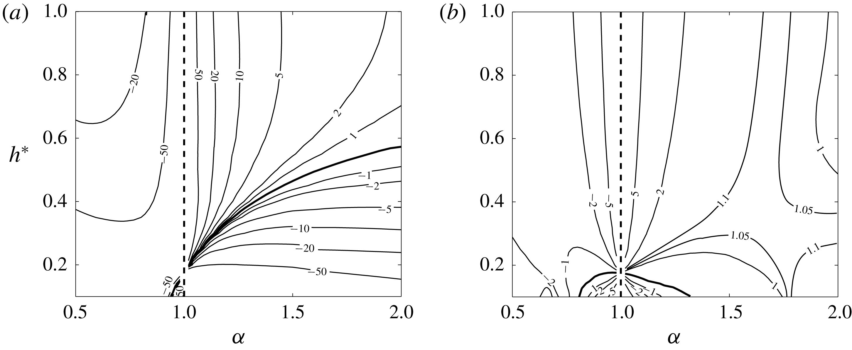
are shown in figure 13. Both contour plots exhibit similar features: a singularity line
 $\unicode[STIX]{x1D6FC}=1$
and a single contour where
 $\unicode[STIX]{x1D6FA}$
and
 $W$
vanish. These zero level contours are different for
 $\unicode[STIX]{x1D6FA}$
and
 $W$
but both cross the singular line
 $\unicode[STIX]{x1D6FC}=1$
at the same value (here
 $h^{\ast }\approx 0.175$
). This special point on the singular line
 $\unicode[STIX]{x1D6FC}=1$
corresponds to the particular solution obtained by Walther et al. (Reference Walther, Guénot, Machefaux, Rasmussen, Chatelain, Okulov, Sørensen, Bergdorf and Koumoutsakos2007). For these parameters, the vortices are undeformed helices of the same pitch. There therefore exist infinitely many frames where the helices are stationary as any values of axial speed
 $W_{a}$
and angular velocity
 $\unicode[STIX]{x1D6FA}_{a}$
can be added provided (2.7) is satisfied. This explains the degeneracy observed at this point in figure 13. These qualitative features do not depend on
 $\unicode[STIX]{x1D700}$
and
 $R^{\ast }$
. It is interesting to note that a contour of
 $\unicode[STIX]{x1D6FA}$
may cross twice a contour of
 $W$
(look at the saddle point region close to
 $(\unicode[STIX]{x1D6FC},h)\approx (1.7,0.4)$
). The coordinates of the two crossing points then correspond to couples of parameters
 $(\unicode[STIX]{x1D6FC},h)$
having the same frame velocities
 $(\unicode[STIX]{x1D6FA},W)$
.
Contour values of the frame velocity in the
 $(\unicode[STIX]{x1D6FC},h)$
plane for
 $R^{\ast }=0.5$
,
 $\unicode[STIX]{x1D700}=0.03$
,
 $N=1$
and
 $\unicode[STIX]{x1D705}=1$
. (a) Angular velocity
 $\unicode[STIX]{x1D6FA}=\unicode[STIX]{x1D6FA}_{F}R_{ext}^{2}/\unicode[STIX]{x1D6E4}$
. (b) Axial velocity
 $W=W_{F}R_{ext}/\unicode[STIX]{x1D6E4}$
. The dashed line (
 $\unicode[STIX]{x1D6FC}=1$
) indicates a line where
 $\unicode[STIX]{x1D6FA}$
and
 $W$
are not defined. The thick solid curve corresponds to the level zero.
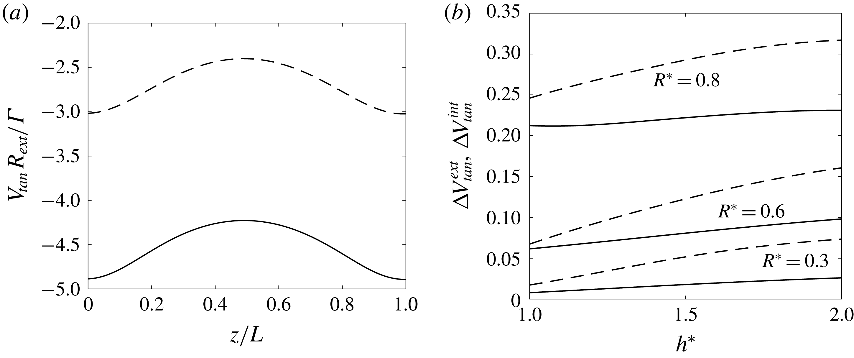
By construction, the vortex elements are advected along the stationary vortex structure. This tangential velocity is different for the internal and the external vortices and varies along the vortex structure, as illustrated in figure 14(a). This variation is associated with the deformation of the helices. It is then important when the level of deformation is high. For each vortex, we define a mean tangential velocity
 $\bar{V}_{tan}$
and a measure
 $\unicode[STIX]{x0394}V_{tan}$
of the fluctuation around this mean using
 $$\begin{eqnarray}\displaystyle \bar{V}_{tan}=\frac{1}{L}\int _{z_{0}}^{z_{0}+L}V_{tan}(z)\,\text{d}z,\quad \unicode[STIX]{x0394}V_{tan}=\frac{\max |V_{tan}-\bar{V}_{tan}|}{|\bar{V}_{tan}|}. & & \displaystyle\end{eqnarray}$$
The measures
 $\unicode[STIX]{x0394}V_{tan}^{ext}$
and
 $\unicode[STIX]{x0394}V_{tan}^{int}$
for the external and internal vortices are plotted as a function of
 $h^{\ast }$
in figure 14(b) for a few cases. We do observe an increase of the tangential velocity fluctuation with
 $h^{\ast }$
and
 $R^{\ast }$
, in agreement with the increase of the vortex deformation (see figure 10).
(a) Variation of the tangential velocity on a period in the internal vortex (dashed line) and in the external vortex (solid line) for a typical case (
 $R^{\ast }=0.6$
,
 $h^{\ast }=1.5$
,
 $\unicode[STIX]{x1D6FC}=1.4$
and
 $\unicode[STIX]{x1D700}=0.03$
,
 $N=1$
,
 $\unicode[STIX]{x1D705}=1$
). (b) Maximum tangential velocity fluctuation in the internal vortex (dashed lines) and external vortex (solid lines) as a function of
 $h^{\ast }$
for different values of
 $R^{\ast }$
and
 $\unicode[STIX]{x1D6FC}=1.4$
,
 $\unicode[STIX]{x1D700}=0.03$
,
 $N=1$
,
 $\unicode[STIX]{x1D705}=1$
.
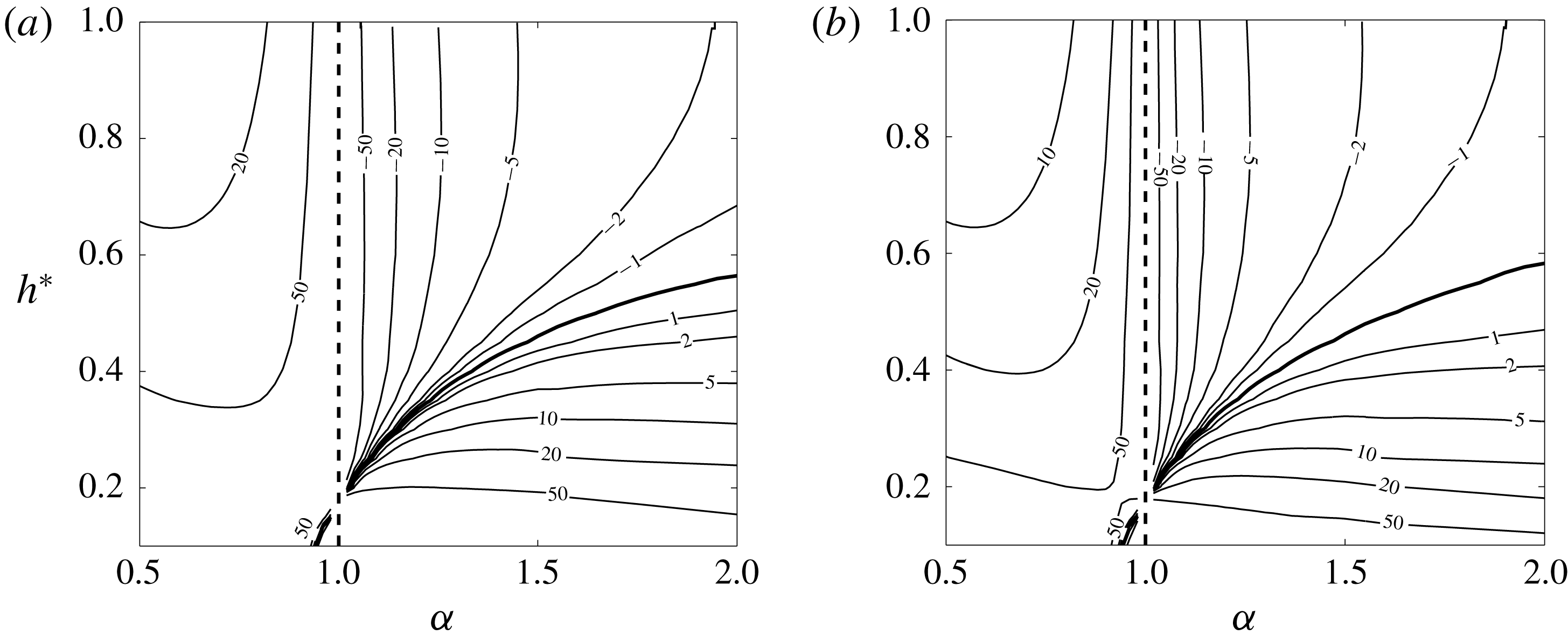
The mean tangential velocity of each vortex is shown in the
 $(\unicode[STIX]{x1D6FC},h)$
plane in figure 15. A positive value corresponds to an advection in the positive axial direction, a negative value to an advection in the opposite direction. Not surprisingly, the mean tangential velocity blows up as
 $\unicode[STIX]{x1D6FC}\rightarrow 1$
like
 $\unicode[STIX]{x1D6FA}_{F}$
and
 $W_{F}$
. It is also interesting to note that the contour curves are similar (in shape) for both vortices and close to those obtained for
 $\unicode[STIX]{x1D6FA}_{F}R_{ext}^{2}/\unicode[STIX]{x1D6E4}$
in figure 13(a).
Contour values of the mean tangential velocities in the
 $(\unicode[STIX]{x1D6FC},h)$
plane for
 $R^{\ast }=0.5$
,
 $\unicode[STIX]{x1D700}=0.03$
,
 $N=1$
,
 $\unicode[STIX]{x1D705}=1$
. (a) External vortex:
 $\bar{V}_{tan}^{ext}R_{ext}/\unicode[STIX]{x1D6E4}$
. (b) Internal vortex:
 $\bar{V}_{tan}^{int}R_{ext}/\unicode[STIX]{x1D6E4}$
. The dashed line (
 $\unicode[STIX]{x1D6FC}=1$
) indicates a line where
 $\bar{V}_{tan}^{ext}$
and
 $\bar{V}_{tan}^{int}$
are not defined. The thick solid curve corresponds to the level zero.
In figure 16(a), we have displayed on the same plot the parameters for which mean tangential velocities and
 $\unicode[STIX]{x1D6FA}_{F}$
vanish. We clearly see that mean tangential velocities and
 $\unicode[STIX]{x1D6FA}_{F}$
vanish for almost the same parameters. This means that there is a very small region of parameters around the line
 $\unicode[STIX]{x1D6FA}_{F}=0$
where internal and external vortices propagate in different directions. This region is delimited by the solid lines shown in figure 16(a). Everywhere else, both vortices propagate in the same direction. We shall see in § 5 that this condition on the direction of propagation of the vortices is necessary for the solution to describe the flow generated by a rotor.
(a) Value of
 $h^{\ast }$
versus
 $\unicode[STIX]{x1D6FC}$
for which
 $\unicode[STIX]{x1D6FA}_{F}=0$
(black dashed line),
 $\bar{V}_{tan}^{ext}=0$
(blue line),
 $\bar{V}_{tan}^{int}=0$
(red line) for
 $R^{\ast }=0.5$
,
 $\unicode[STIX]{x1D700}=0.03$
,
 $N=1$
,
 $\unicode[STIX]{x1D705}=1$
. (b) Comparison of mean tangential velocity
 $\bar{V}_{tan}$
(solid lines) and tangential frame velocity
 $V_{Ftan}$
(dashed lines) for external and internal vortices (normalized by
 $\unicode[STIX]{x1D6E4}/R_{ext}$
). Parameters are
 $R^{\ast }=0.5$
,
 $\unicode[STIX]{x1D6FC}=1.2$
,
 $\unicode[STIX]{x1D700}=0.03$
,
 $N=1$
,
 $\unicode[STIX]{x1D705}=1$
.
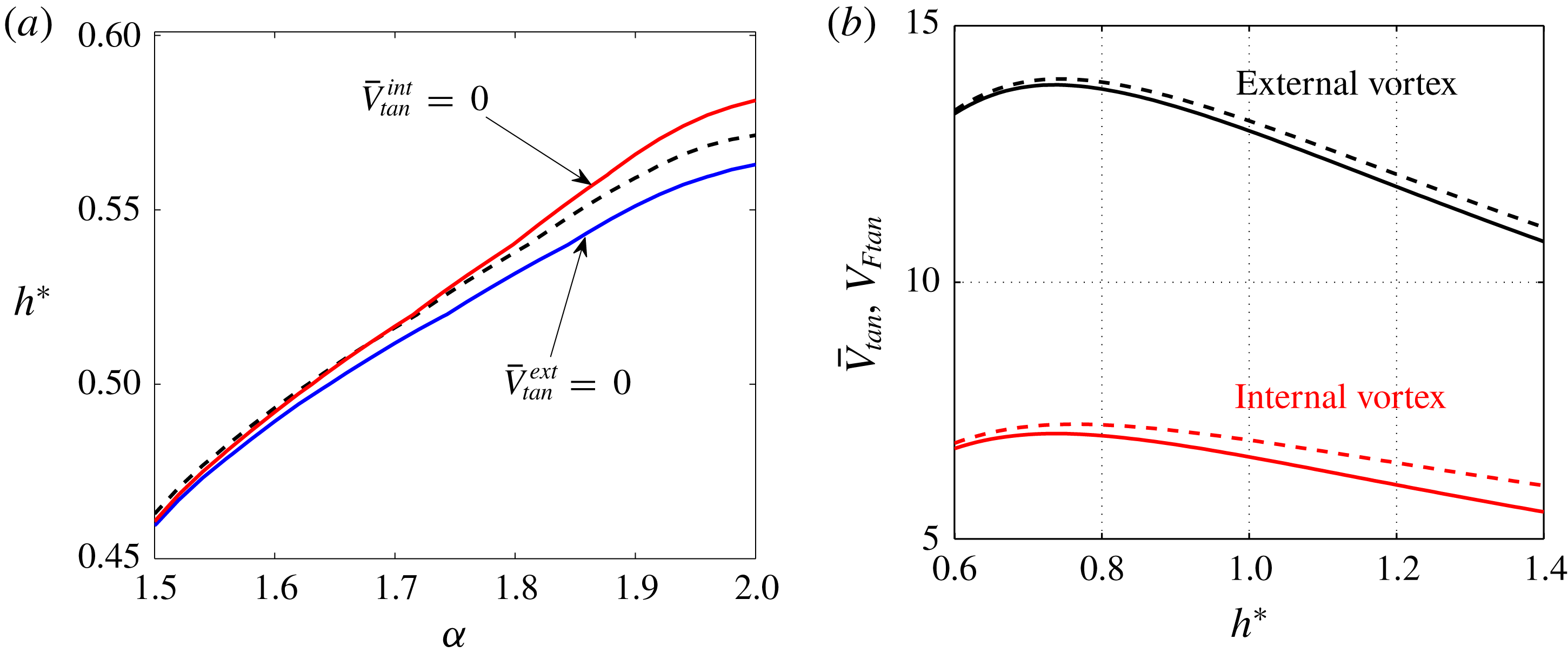
It is interesting to compare more precisely the mean tangential velocity with the velocity associated with the moving frame. Assuming that each structure is approximatively a helix, this tangential ‘frame’ velocity is given by
 $$\begin{eqnarray}\displaystyle V_{Ftan}^{int}=-\frac{\unicode[STIX]{x1D6FA}_{F}R_{ext}R^{\ast }+W_{F}h^{\ast }/(2\unicode[STIX]{x03C0}\unicode[STIX]{x1D6FC}R^{\ast })}{\sqrt{1+{h^{\ast }}^{2}/(2\unicode[STIX]{x03C0}\unicode[STIX]{x1D6FC}R^{\ast })^{2}}},\quad V_{Ftan}^{ext}=-\frac{\unicode[STIX]{x1D6FA}_{F}R_{ext}+W_{F}h^{\ast }/(2\unicode[STIX]{x03C0})}{\sqrt{1+{h^{\ast }}^{2}/(2\unicode[STIX]{x03C0})^{2}}} & & \displaystyle\end{eqnarray}$$
for the internal and external vortices, respectively. The difference between
 $V_{Ftan}$
and
 $\bar{V}_{tan}$
is associated with the vortex induction. In figure 16(b), we can observe the similar values of
 $\bar{V}_{tan}$
and
 $V_{Ftan}$
in the whole range of
 $h^{\ast }$
between 0.6 and 1.4 for a typical case. This means that the most important part of the tangential velocity is associated with the frame velocity and the vortex induction contribution remains in general small.
3.4 Induced flow
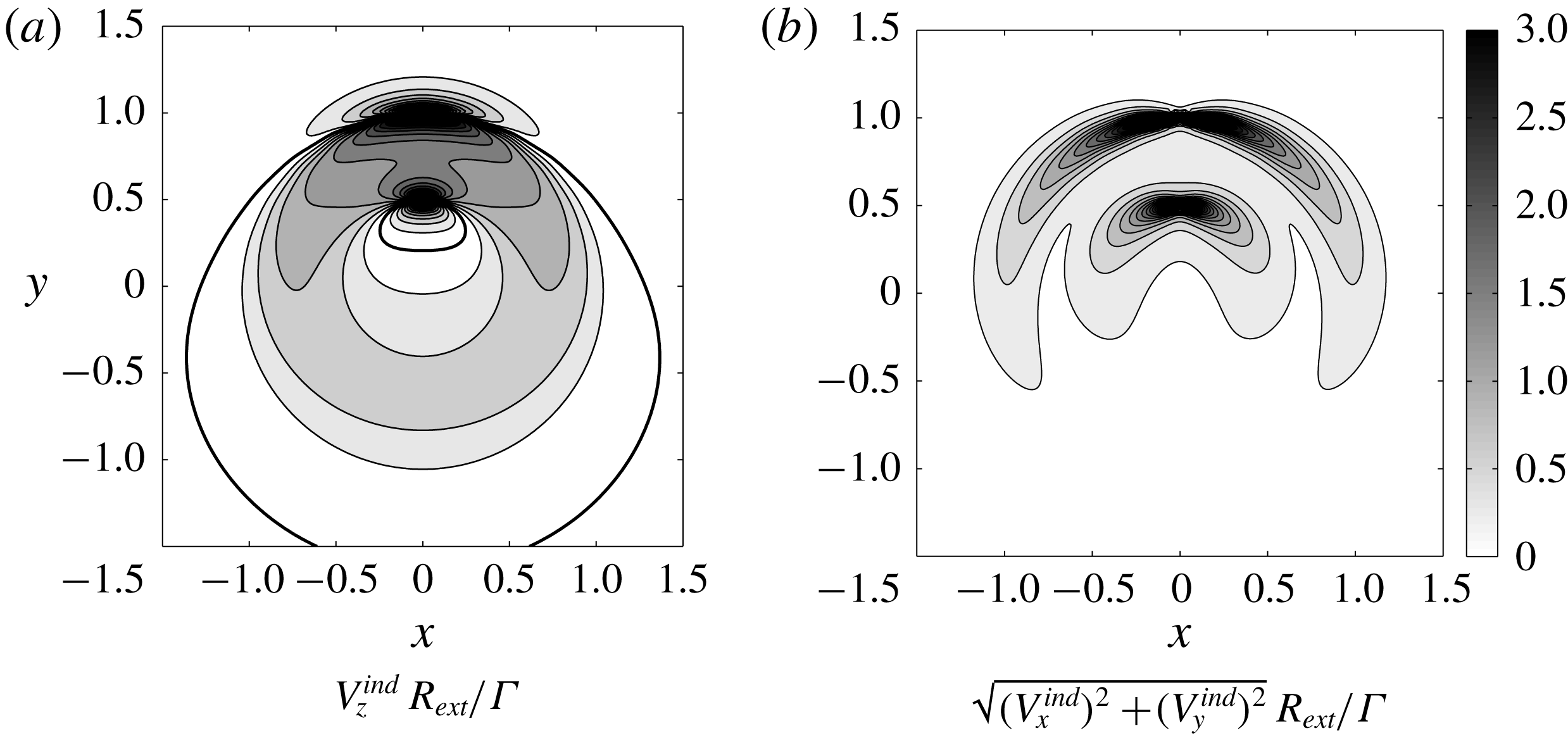
From the point of view of applications, it is useful to know the velocity field induced by the vortex structure. An illustration of the axial and angular components of such a field in a plane perpendicular to the structure axis is shown in figure 17. In these contour plots, the axial velocity
 $W_{F}$
and angular velocity
 $\unicode[STIX]{x1D6FA}_{F}$
have been subtracted such that the velocity field vanishes far from the centre. The vortex cores where the velocity field is smoothed have also been indicated. We clearly see that the induced velocity field exhibits strong inhomogeneities.
Induced velocity contours in a cross-section (
 $z=0$
plane) for
 $h^{\ast }=1$
,
 $R^{\ast }=0.5$
,
 $\unicode[STIX]{x1D6FC}=1.5$
,
 $\unicode[STIX]{x1D700}=0.03$
,
 $N=1$
and
 $\unicode[STIX]{x1D705}=1$
. In (a) colours are for
 $|V_{z}^{ind}|$
with the same colour map as in (b).
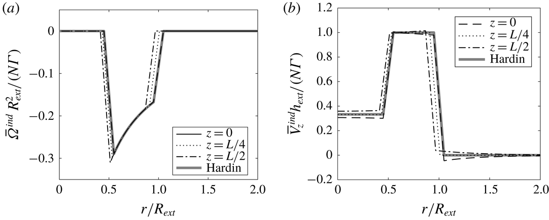
Azimuthally averaged induced velocity profile for the same parameters as in figure 17. Solid lines: numerical results at different axial locations. Dashed line: theoretical prediction for perfect helices using the Hardin model. (a) Angular velocity
 $\bar{\unicode[STIX]{x1D6FA}}^{ind}R_{ext}^{2}/(N\unicode[STIX]{x1D6E4})$
. (b) Axial velocity
 $\bar{V}_{z}^{ind}h_{ext}/(N\unicode[STIX]{x1D6E4})$
.
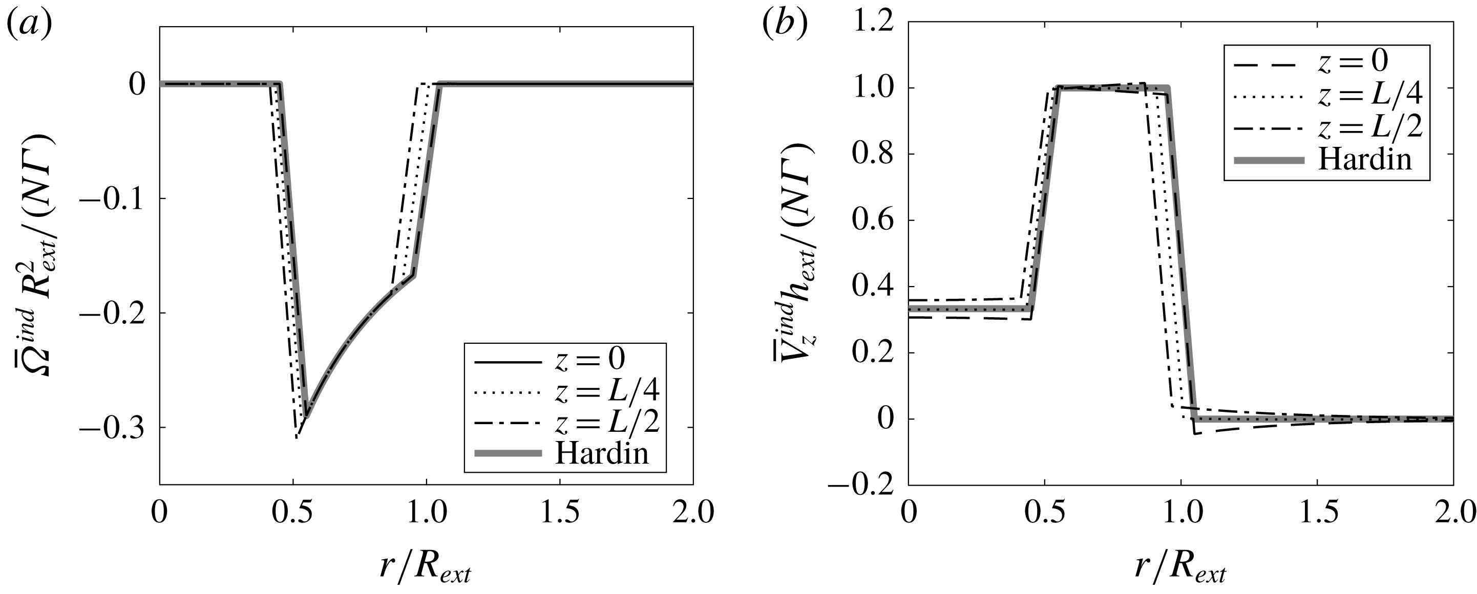
In figure 18, we show the azimuthally averaged flow versus
 $r$
at different axial locations. In the core region of each vortex (at a distance smaller than
 $a$
from the vortex centre), each velocity profile has been replaced by a linear fit. We do see small fluctuations of the profiles between different locations but the profiles remain close to the profiles generated by
 $N$
pairs of perfect helices. These ideal profiles are given (for infinitely thin vortices) by Hardin (Reference Hardin1982)
 $$\begin{eqnarray}\displaystyle & \displaystyle \bar{V}_{z}^{H}=\displaystyle \frac{N\unicode[STIX]{x1D6E4}}{h_{ext}}\left\{\begin{array}{@{}ll@{}}1-\displaystyle \frac{1}{\unicode[STIX]{x1D6FC}} & \text{if }r<R_{int},\\ 1 & \text{if }R_{int}<r<R_{ext},\\ 0 & \text{if }r>R_{ext},\end{array}\right. & \displaystyle\end{eqnarray}$$
 $$\begin{eqnarray}\displaystyle & \displaystyle \bar{\unicode[STIX]{x1D6FA}}^{H}=\displaystyle \frac{N\unicode[STIX]{x1D6E4}}{R_{ext}^{2}}\left\{\begin{array}{@{}ll@{}}-\displaystyle \frac{R_{ext}^{2}}{2\unicode[STIX]{x03C0}r^{2}} & \text{if }R_{int}<r<R_{ext},\\ 0 & \text{elsewhere}.\end{array}\right. & \displaystyle\end{eqnarray}$$
The fluctuations are mainly associated with the radial displacement of the vortices. When the helices are less deformed, the fluctuations are smaller. It is interesting to note that the azimuthally averaged axial flow changes sign close to the axis when
 $h_{int}<h_{ext}$
, that is
 $\unicode[STIX]{x1D6FC}<1$
.
For the applications, it is also useful to evaluate the mass flow rate induced by the structure. The mass axial flow rate is defined by
 $$\begin{eqnarray}\displaystyle M=\iint \unicode[STIX]{x1D70C}V_{z}^{ind}r\,\text{d}r\,\text{d}\unicode[STIX]{x1D719}. & & \displaystyle\end{eqnarray}$$
For
 $N$
undeformed helical pairs, we get using (3.8)
 $$\begin{eqnarray}\displaystyle M^{H}=\unicode[STIX]{x1D70C}N\unicode[STIX]{x1D6E4}\unicode[STIX]{x03C0}\left(\frac{R_{ext}^{2}}{h_{ext}}-\frac{R_{int}^{2}}{h_{int}}\right), & & \displaystyle\end{eqnarray}$$
that is
 $$\begin{eqnarray}\displaystyle \frac{M^{H}}{\unicode[STIX]{x1D70C}N\unicode[STIX]{x1D6E4}R_{ext}}=\frac{\unicode[STIX]{x03C0}}{h^{\ast }}\left(1-\frac{(R^{\ast })^{2}}{\unicode[STIX]{x1D6FC}}\right). & & \displaystyle\end{eqnarray}$$
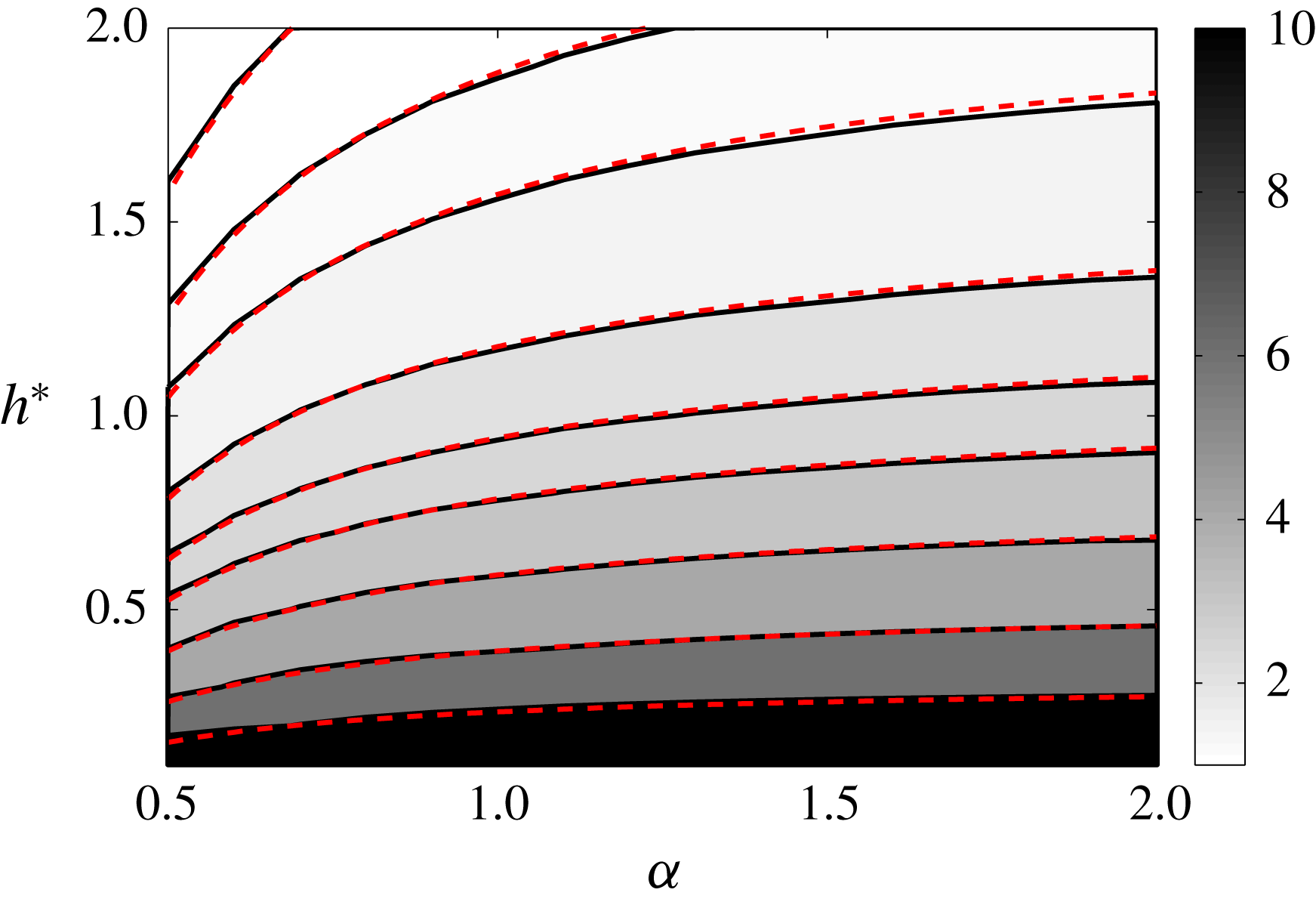
This expression provides a good approximation of the mass flow rate of the deformed structure, as observed in figure 19 for a typical example.
Contours of mass axial flow rate
 $M$
(normalized by
 $\unicode[STIX]{x1D70C}N\unicode[STIX]{x1D6E4}R_{ext}$
) in the
 $(\unicode[STIX]{x1D6FC},h)$
plane for
 $R^{\ast }=0.5$
,
 $\unicode[STIX]{x1D700}=0.03$
,
 $N=1$
and
 $\unicode[STIX]{x1D705}=1$
. Contours correspond from top to bottom to
 $\{1,1.25,1.5,2,2.5,3,4,6,10\}$
. Solid lines:
 $M$
; red dashed lines:
 $M^{H}$
.
Note that
 $M^{H}$
changes sign when
 $\unicode[STIX]{x1D6FC}<(R^{\ast })^{2}$
. In this regime, the induced axial flow is sufficiently negative close to the axis to invert the positive mass flow rate occurring between the internal and external vortices. For the parameters of figure 19, this is expected for very small
 $\unicode[STIX]{x1D6FC}$
(
 $\unicode[STIX]{x1D6FC}<0.25$
).
4 Analysis of the effect of a varying core size
We have seen that the tangential velocity varies along each vortex structure when it is deformed. This implies that each vortex experiences a stretching field that in principle induces a variation of its core size. In this section, our objective is to quantify this effect.
In a inviscid framework, the way the core size varies is simply given by the conservation of the mass flux in the vortex core which imposes
 $$\begin{eqnarray}\displaystyle a^{2}V_{tan}=\text{Cst}. & & \displaystyle\end{eqnarray}$$
As soon as
 $a$
changes, the self-induced velocity is modified and therefore a different equilibrium solution is obtained.
In figure 20, we have analysed the effect of a varying core size in an extreme case (
 $R^{\ast }=0.8$
,
 $h^{\ast }=1.4$
,
 $\unicode[STIX]{x1D700}=0.03$
,
 $\unicode[STIX]{x1D6FC}=1.4$
,
 $N=1$
,
 $\unicode[STIX]{x1D705}=1$
). As seen in figure 14(b), for this value of
 $R^{\ast }$
, the variations of
 $V_{tan}$
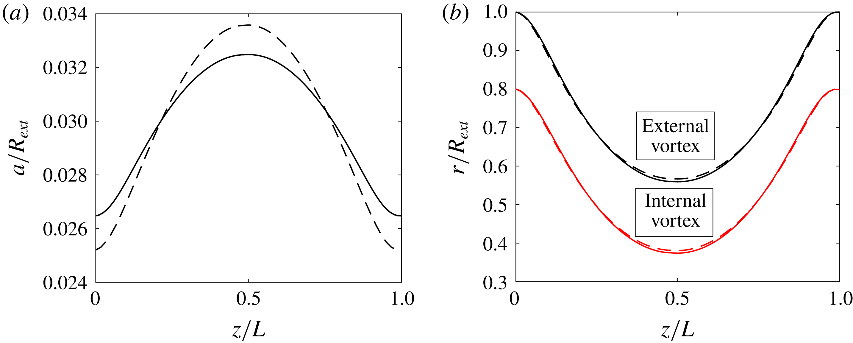
are the largest: they reach 32 % for the internal vortex, and 23 % for the external one. In figure 20(a), we have plotted the variation of the core size in a period for the converged solution in both vortices. The variations of the core size are weaker than those of the tangential velocity, as expected from (4.1). They are approximately 10 % for the internal vortex, and 7 % for the external vortex, with respect to the mean core size
 $a=0.03$
. In figure 20(b), the radial position of the vortices is shown. The solution with a varying core size is compared to the solution with a constant core size. We observe that the difference between both solutions is very small. The largest gaps between both radial positions are 0.78 % and 0.66 % for the internal and external vortex, respectively. In terms of moving frame velocities, the differences are also extremely small: we obtain the values
 $W=1.826$
and
 $\unicode[STIX]{x1D6FA}=3.697$
for a varying core size, while we had
 $W=1.809$
and
 $\unicode[STIX]{x1D6FA}=3.610$
for a constant core size.
This comparison guarantees that the effects of a varying core size is negligible for all the cases that we have considered. It a posteriori justifies the use of the approximation of a constant core size in our work.
(a) Variation of the core size
 $a/R_{ext}$
for the external (solid line) and internal (dashed line) vortices. The mean core size value in each vortex is
 $a/R_{ext}=0.03$
. (b) Radial position of the internal and external vortices for a constant core size (dashed line) and for a variable core size obtained using (4.1) (solid line). The parameters in both panels are
 $R^{\ast }=0.8$
,
 $h^{\ast }=1.4$
,
 $\unicode[STIX]{x1D6FC}=1.4$
,
 $N=1$
,
 $\unicode[STIX]{x1D705}=1$
and a mean core size
 $a/R_{ext}=0.03$
.
5 Discussion in the context of rotors
In this section, we discuss our solutions in the context of rotor wakes. Our objective is to identify, as a function of the geometrical parameters, which far wake situations the solutions could possibly describe. In other words, if a solution was able to represent the flow generated by rotor, which rotor configuration it would be.
In the previous sections, we have obtained the frame where each solution is stationary. If the flow was created by a rotor, this frame would necessarily be a frame attached to a blade. In other words, the angular velocity
 $-\unicode[STIX]{x1D6FA}_{F}$
would be the rotation rate of the rotor and
 $-W_{F}$
the external wind velocity. Moreover, in the far field, the vortices which have been created by the rotor would have to move away from it. From the direction of propagation of the vortices, which is given by the sign of the mean tangential velocity, we can then deduce the side where the rotor should be. For example, if
 $\bar{V}_{tan}>0$
, the vortices move in the positive direction, the rotor should then be located on the negative side.
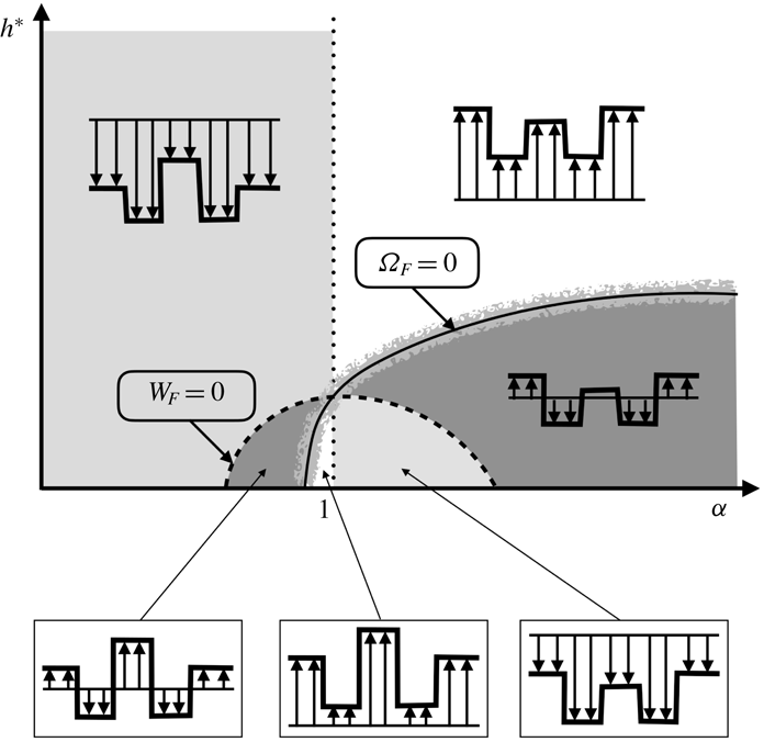
Diagram of the different rotor flow regimes. White regions: windmill brake regime or wind turbine regime (both vortices are going upwards as the external wind). Light grey regions: ascending regime (both vortices are going downwards as the external wind). Dark grey regions: slow descending regime and vortex ring state (both vortices are going downwards while the external wind is going upwards). Close to the line
 $\unicode[STIX]{x1D6FA}_{F}=0$
, there exists a small region where one vortex is going upwards while the other is going downwards: such a solution cannot describe the (far) wake of a rotor.
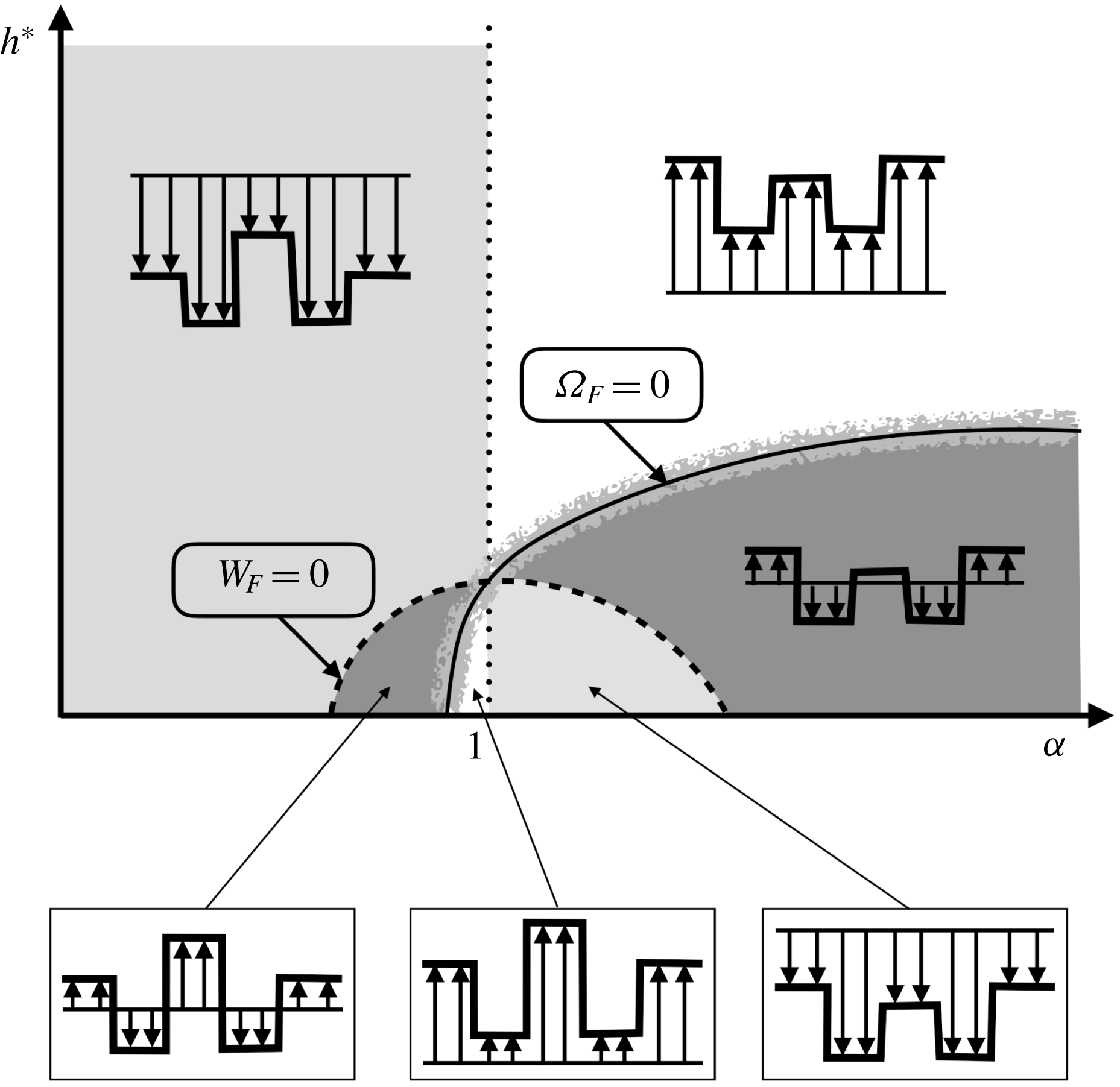
By analysing the directions of propagation of the vortices and of the external wind, one can build the diagram shown in figure 21. The different domains are limited by the curves
 $W_{F}=0$
and
 $\unicode[STIX]{x1D6FA}_{F}=0$
and the line
 $\unicode[STIX]{x1D6FC}=1$
, which correspond to changes of the signs of the direction of propagation of the vortices or of the external wind. In this figure, we have also indicated the typical azimuthally averaged axial flow corresponding to each regime. For example, in the white region on the right of the line
 $\unicode[STIX]{x1D6FC}=1$
,
 $W_{F}>0$
,
 $\bar{V}_{tan}^{ext}<0$
,
 $\bar{V}_{tan}^{int}<0$
and
 $M>0$
: both vortices move in the same negative direction as the external wind, which is opposite to the direction of the mass flow rate. Assuming a positive axis downwards, this situation corresponds to the so-called windmill brake regime of an helicopter: the helicopter is going downwards, while the flow and the vortices are going upwards with respect to the helicopter rotor. This regime also corresponds to the wind turbine regime. The difference compared to the other windmill brake regime obtained for
 $\unicode[STIX]{x1D6FC}<1$
is in the azimuthally averaged axial flow, which is stronger than the external wind close to the axis in that case.
In the light grey regions, the vortex velocities are positive while
 $W_{F}<0$
. This regime corresponds to a climbing regime: the vortices move downwards as do the external flow and the mass flow rate. In the dark grey regions,
 $W_{F}$
and the vortex velocities are positive as is the mass flow rate. This situation corresponds to a slow descending regime: the vortices move downwards while the external flow goes upwards. It does not tell us anything on the behaviour of the vortices close to the rotor. It is not excluded that the vortices exhibit a complex pattern near the rotor, as observed in the so-called vortex ring state (Drees & Hendal Reference Drees and Hendal1951; Quaranta Reference Quaranta2017; Durán Venegas & Le Dizès Reference Durán Venegas and Le Dizès2018).
Note that the curve
 $\unicode[STIX]{x1D6FA}_{F}=0$
is not exactly the limit between the windmill brake regime and the slow descending regime. There is actually a small region close to this curve where the solution cannot correspond to any helicopter flight regime. This region has been displayed in figure 16(a) for a particular set of parameters. In this region, internal and external vortices move in opposite directions. For this reason, they cannot be created by a single rotor located far away.
6 Conclusion
We have obtained new numerical solutions that extend the uniform helices that are usually used to describe the far wake generated by a rotor in axial wind. These solutions are spatially periodic and steady in a rotating and translating frame. They describe a situation where each blade creates two counter-rotating vortices emitted at two different non-vanishing radii. We have shown that these solutions can be considered as deformed helices. They exhibit radial variations that increase as the internal vortex gets closer to the external vortex. We have provided simpler numerical solutions that capture the main features of the solutions. We have also considered the variation of the vortex core size associated with the deformation and shown that it has a very weak effect on the main characteristics of the solutions. Finally, we have addressed the relevance of these solutions for the far wake description of helicopters in vertical displacement.
The stability of the solutions has not been considered. Long-wavelength instability is known to affect single helices (Widnall Reference Widnall1972; Quaranta, Bolnot & Leweke Reference Quaranta, Bolnot and Leweke2015) as well as multiple helices (Gupta & Loewy Reference Gupta and Loewy1974; Okulov Reference Okulov2004; Selçuk, Delbende & Rossi Reference Selçuk, Delbende and Rossi2017a ; Quaranta Reference Quaranta2017). Similar instabilities are expected to exist in the present solutions.
Note finally that we have not considered the inner structure of the vortices. Fukumoto & Okulov (Reference Fukumoto and Okulov2005) and Blanco-Rodríguez et al. (Reference Blanco-Rodríguez, Le Dizès, Selçuk, Delbende and Rossi2015) among others have shown that the cores of helical vortices deform due to the effects of curvature, torsion and strain. These deformations are responsible of short-wavelength instabilities that develop in vortex cores. Local curvature induces the curvature instability (Hattori & Fukumoto Reference Hattori and Fukumoto2014; Blanco-Rodríguez & Le Dizès Reference Blanco-Rodríguez and Le Dizès2017) while strain causes the elliptic instability (Blanco-Rodríguez & Le Dizès Reference Blanco-Rodríguez and Le Dizès2016). Both instabilities are expected to be present in the inner core of our solutions.
Acknowledgements
This work received support from the French Agence Nationale de la Recherche under the A*MIDEX grant ANR-11-IDEX-0001-02, the LABEX MEC project ANR-11-LABX-0092 and the ANR TWIN-HELIX project ANR-17-CE06-0018-01. E.D.V. also acknowledge DGA and Aix Marseille Université for his PhD grant.
Appendix A. Asymptotic expressions of
 $\unicode[STIX]{x1D6FA}$
and
$W$
for a single helix


The angular rotation
 $\unicode[STIX]{x1D6FA}$
and the axial velocity
 $W$
of a fluid element on a helix of pitch
 $h$
, radius
 $R$
, core size
 $a$
and circulation
 $\unicode[STIX]{x1D6E4}$
are given by the expressions
 $$\begin{eqnarray}\displaystyle & \displaystyle \displaystyle \frac{\unicode[STIX]{x1D6FA}R^{2}}{\unicode[STIX]{x1D6E4}}=\displaystyle \frac{\ln (2/\unicode[STIX]{x1D716})+2(1+p^{2})-\ln (\sqrt{1+p^{2}})-(1+p^{2})^{3/2}[2/p-{\mathcal{W}}(p)]-1/4}{4\unicode[STIX]{x03C0}(1+p^{2})^{3/2}}, & \displaystyle\end{eqnarray}$$
 $$\begin{eqnarray}\displaystyle & \displaystyle \frac{WR}{\unicode[STIX]{x1D6E4}}=\frac{\ln (2/\unicode[STIX]{x1D716})-\ln (\sqrt{1+p^{2}})+(1+p^{2})^{3/2}{\mathcal{W}}(p)-1/4}{4\unicode[STIX]{x03C0}(1+p^{2})^{3/2}}, & \displaystyle\end{eqnarray}$$
 $p=h/(2\unicode[STIX]{x03C0}R)$
,
 $\unicode[STIX]{x1D716}=a/[R(1+p^{2})]$
and
 ${\mathcal{W}}(p)$
is the function defined in Boersma & Wood (Reference Boersma and Wood1999) by
 $$\begin{eqnarray}\displaystyle {\mathcal{W}}(p)=\int _{0}^{\infty }\left\{\frac{\sin ^{2}t}{(p^{2}t^{2}+\sin ^{2}t)^{3/2}}-\frac{1}{(p^{2}+1)^{3/2}}\frac{H(1/2-t)}{t}\right\}\,\text{d}t. & & \displaystyle\end{eqnarray}$$
These expressions are (2.13) and (2.15) of Velasco Fuentes (Reference Velasco Fuentes2018) corrected by a
 $1/4$
term to account for the vortex deformation induced by curvature. This term is obtained by projecting in the azimuthal and axial directions a correction derived for the bi-normal velocity component by Boersma & Wood (Reference Boersma and Wood1999). The correction terms that would come from the tangential velocity component have never been computed, but we suspect that they are
 $O(\unicode[STIX]{x1D716})$
.
In formulas (A 1a,b
), it is implicitly assumed that the vortex core model is a Rankine vortex (uniform vortex). Using another vortex model amounts to change the definition of the vortex core size
 $a$
as explained by Widnall (Reference Widnall1972) (see also Saffman Reference Saffman1992).