



1. Introduction
The interaction between disturbances and shock waves constitutes a fundamental problem in compressible fluid dynamics, with direct relevance to a broad range of high-speed flow phenomena (Tam & Tanna Reference Tam and Tanna1982; Zhang et al. Reference Zhang, Han, Tang, Qu and Yan2025). When turbulence passes through a shock wave, velocity fluctuations are significantly amplified and length scales are substantially altered, profoundly affecting turbulent mixing and flow structure (Andreopoulos et al. Reference Andreopoulos, Agui and Briassulis2000). A paradigmatic example is high-speed boundary-layer receptivity (Ma & Zhong Reference Ma and Zhong2005; Fedorov Reference Fedorov2011; Wan et al. Reference Wan, Luo and Su2018): small disturbances in the free stream first interact with the bow shock and subsequently excite boundary-layer instability waves. Characterising the post-shock disturbance field is therefore a prerequisite for understanding the receptivity mechanisms. In both contexts, exact analytical solutions offer valuable insight into the fundamental physics governing such interactions.
A canonical simplified model for this disturbance–shock interaction assumes a planar zero-thickness shock interacting with small-amplitude disturbances, allowing the Rankine–Hugoniot relations to be linearised. This linear interaction approximation (LIA) then predicts turbulence amplification when upstream fluctuations are sufficiently small that the shock front remains undisplaced (Anyiwo & Bushnell Reference Anyiwo and Bushnell1982; Ribner Reference Ribner1987). For boundary-layer receptivity on flight vehicles, this model is justified downstream of the nose region, where the shock can be treated as locally planar because of its small curvature and wall effects are negligible due to the large distance from the wall. In a compressible uniform flow, small disturbances can always be decomposed into three fundamental modes (Kovásznay Reference Kovásznay1953): acoustic, entropy and vorticity waves. Although turbulence deals with random statistical disturbances while receptivity concerns deterministic modal waves, they share the same essential core: determining the induced disturbances and shock oscillations resulting from incident waves.
Within this linearised framework, early theoretical studies primarily examined planar shock interactions with specific types of incident waves. Ribner (Reference Ribner1954) investigated shear waves with arbitrary spatial distributions propagating through a planar normal shock, showing that they refract and change amplitude while inducing downstream pressure disturbances. Moore (Reference Moore1953) extended this framework to planar disturbances impinging on a normal shock from arbitrary directions, including downstream acoustic waves. He demonstrated that attenuated pressure waves (evanescent waves) arise downstream in the absence of upstream propagating acoustic modes. Kerrebrock (Reference Kerrebrock1956) analysed interactions between random small disturbances and shock waves or flame fronts in compressible fluids, proposing that the post-shock disturbance field consists of pressure, entropy and vorticity fluctuations whose characteristics evolve upon passing through shocks or flames. D’Iakov (Reference D’iakov1958a ; Reference D’Iakov1958b ) computed the effects of small disturbances on both sides of an oblique shock wave, noting that the linear approximation fails when the incoming flow Mach number reaches a critical value.
Building upon these earlier studies, Mckenzie & Westphal (Reference Mckenzie and Westphal1968) drew an analogy between the refraction of incident disturbances at a shock wave and Snell’s law in optics. They derived analytical expressions for the amplitudes of transmitted waves resulting from incident waves of arbitrary type and direction, thereby establishing a comprehensive theoretical framework for predicting the post-shock disturbance field. Notably, they found that acoustic waves incident beyond a critical angle cease to propagate; however, their analysis, being confined to real wavenumbers, could not provide solutions for these non-propagating disturbances. Subsequent analysis by Robinet & Casalis (Reference Robinet and Casalis2001) identified this critical angle as corresponding to a singular point in the linearised Euler equations, where the eigenvalues of two acoustic modes coincide. To resolve the limitation of real-wavenumber analysis, Huang & Wang (Reference Huang and Wang2019) introduced complex wavenumbers in the post-shock region, obtaining evanescent solutions which they termed ‘damping waves’. Nevertheless, the physical interpretation of these waves remained ambiguous.
In parallel, this linear interaction analysis has been widely employed for stochastic turbulent fields passing through a shock wave, providing key information on the direct effect caused solely by the Rankine–Hugoniot relations. By decomposing the upstream turbulence into three independently evolving fundamental modes, the downstream statistical field is reconstructed by integrating over all orientations of the pre-shock wave vector. This approach has been applied to isotropic vorticity (Wouchuk et al. Reference Wouchuk, Huete and Velikovich2009), density (Huete et al. Reference Huete, Velikovich and Wouchuk2011) and acoustic (Huete et al. Reference Huete, Wouchuk and Velikovich2012) fluctuations, yielding predictions for post-shock turbulent kinetic energy, acoustic radiation and vorticity amplification. More recently, this linear analysis has been extended to accommodate real gas thermodynamic effects, such as the Noble–Abel stiffened gas model, enabling its application to high-pressure dense fluid conditions beyond the ideal gas assumption (Farag et al. Reference Farag, Boivin and Sagaut2023). High fidelity numerical simulations have validated these linear predictions in shock–isotropic turbulence interactions (Hannappel & Friedrich Reference Hannappel and Friedrich1995; Shi et al. Reference Shi, Guo, Liu and Wang2024). This linear framework is also relevant to shock-induced boundary-layer interaction (SBLI) in regions far from the boundary layer, where the shock is approximately planar and the mean flow uniform (Zhang et al. Reference Zhang, Han, Tang, Qu and Yan2025).
Despite these advancements, prior studies universally adopt a temporal perspective in which incident waves are prescribed and the resulting responses are determined. Within this framework, wavenumbers are restricted to real values, inherently excluding evanescent waves. More fundamentally, this approach yields only case-specific solutions rather than a physical picture of the relationship among all the upstream and downstream waves. For instance, it cannot explain how different incident modes relate to one another in producing the same downstream response. Without this relationship, one cannot construct a one-to-one mapping from downstream responses to incident waves. Consequently, the inverse problem – determining the incident disturbance required to achieve a prescribed downstream response – cannot be addressed. These issues are particularly important for boundary-layer receptivity, as resolving them reveals how different free stream modes are linked and enables potential flow control via tailored post-shock disturbances.
To overcome these limitations, the present study adopts a spatial formulation that admits complex wavenumbers, which naturally accommodate evanescent waves. As will be shown, this spatial approach reveals an intrinsic coupling among different modes across the shock, allowing us to construct a bijective mapping from upstream disturbances to the downstream response, thereby making the inverse problem well-posed. To our knowledge, this inverse formulation has not been recognised in previous work.
The remainder of this paper is organised as follows. Section 2 introduces the governing equations. Section 3 analyses small disturbances in a uniform flow from both temporal and spatial perspectives, elucidating the physical properties of evanescent waves. Section 4 presents the mathematical formulation for matching disturbances across the shock interface, deriving the solutions for both wavenumbers and amplitudes, and defines the inverse problem. Using a Mach 2 normal shock flow as an example, § 5 illustrates the complete solution map, presents the results of the inverse problem and validates the theoretical predictions via direct numerical simulation (DNS). Finally, § 6 summarises the main conclusions.
2. Problem and governing equations
We investigate the interaction of small disturbances with a stationary planar shock wave in a uniform flow, where the normal velocity is supersonic upstream and subsonic downstream. A shock-oriented coordinate system is established (figure 1), with the
 $x$
-axis aligned along the shock normal pointing downstream and the
 $y$
–
 $z$
plane coinciding with the undisturbed shock surface. Subscripts
 ${L}$
and
 ${R}$
denote upstream and downstream quantities, respectively.
Schematic of the flow configuration across a planar shock. The coordinate system is defined with the
 $x$
-axis along the shock normal (pointing downstream) and the
 $y$
–
 $z$
plane coinciding with the undisturbed shock surface. Quantities without and with a tilde denote the base flow and the disturbance fields, respectively.

Figure 1. Long description
A diagram of the flow configuration across a planar shock. The coordinate system is defined with the x-axis along the shock normal pointing downstream and the y-z plane coinciding with the undisturbed shock surface. The diagram is divided into three sections: Upstream (L), Planar shock, and Downstream (R). In the Upstream section, there are symbols representing density, velocity, and pressure, along with a wavy line indicating disturbances. In the Downstream section, similar symbols represent the altered density, velocity, and pressure after passing through the shock. The Planar shock section shows the shock wave as a blue plane intersecting the coordinate axes.
The compressible flow across the shock is governed by the conservation laws of mass, momentum and energy, expressed in conservative form as
 \begin{align} \frac {\partial \boldsymbol{U}}{\partial t} + \frac {\partial \boldsymbol{F}_{\kern-1pt j}}{\partial x_{\kern-1pt j}} = 0, \end{align}
where
 $t$
is time,
 $x_{\kern-1pt j}$
(
 $j = 1,2,3$
) denotes the Cartesian coordinates
 $(x, y, z)$
and summation over repeated index
 $j$
is implied. The conservative variable vector is
 \begin{align} \boldsymbol{U} = (\rho , \rho u_i, \rho E)^{{T}}, \end{align}
where
 $\rho$
is density,
 $u_i$
(
 $i = 1,2,3$
) are the velocity components in the three coordinate directions and
 $E = e + ( {1}/{2})u_k u_k$
is the total energy per unit mass, with
 $e$
as the specific internal energy. The inviscid flux vector in the
 $x_{\kern-1pt j}$
-direction is
 \begin{align} \boldsymbol{F}_{\kern-1pt j} = \big(\rho u_{\kern-1pt j}, \rho u_{\kern-1pt j} u_i + p \delta _{\textit{ji}}, \rho E u_{\kern-1pt j} + p u_{\kern-1pt j} \big)^{{T}}, \end{align}
where
 $p$
is pressure and
 $\delta _{\textit{ij}}$
is the Kronecker delta.
For a calorically perfect gas, the equation of state is
 $p = \rho R T$
, where
 $R$
is the specific gas constant and
 $T$
is temperature, and the internal energy is
 \begin{align} e = \frac {p}{\rho (\gamma - 1)}, \end{align}
where
 $\gamma$
is the specific heat ratio. The energy equation in (2.1) can then be replaced by a pressure transport equation, derived by combining the energy equation with the continuity equation and the equation of state:
 \begin{align} \frac {\partial p}{\partial t} + u_{\kern-1pt j} \frac {\partial p}{\partial x_{\kern-1pt j}} + \gamma p \frac {\partial u_{\kern-1pt j}}{\partial x_{\kern-1pt j}} = 0. \end{align}
To analyse small disturbances, the flow variables
 $\boldsymbol{\varphi } = (\rho , u_i, p)^{{T}}$
are decomposed into base flow components
 $\bar {\boldsymbol{\varphi }}$
and infinitesimal perturbations
 $\tilde {\boldsymbol{\varphi }}$
:
 \begin{align} \boldsymbol{\varphi } = \bar {\boldsymbol{\varphi }} + \tilde {\boldsymbol{\varphi }}. \end{align}
Substituting this decomposition into the conservation equations (2.1) (with the energy equation replaced by (2.5)), subtracting the base flow equations and retaining first-order terms yields the linearised system for perturbations
 $(\tilde {\rho }, \tilde {u}_i, \tilde {p})$
:
 \begin{align} \frac {\partial \tilde {\rho }}{\partial t} + u_{\kern-1pt j} \frac {\partial \tilde {\rho }}{\partial x_{\kern-1pt j}} + \rho \frac {\partial \tilde {u}_j}{\partial x_{\kern-1pt j}} &= 0, \\[-12pt] \nonumber \end{align}
 \begin{align} \rho \frac {\partial \tilde {u}_i}{\partial t} + \rho u_{\kern-1pt j} \frac {\partial \tilde {u}_i}{\partial x_{\kern-1pt j}} + \frac {\partial \tilde {p}}{\partial x_i} &= 0, \\[-12pt] \nonumber \end{align}
 \begin{align} \frac {\partial \tilde {p}}{\partial t} + u_{\kern-1pt j} \frac {\partial \tilde {p}}{\partial x_{\kern-1pt j}} + \gamma p \frac {\partial \tilde {u}_j}{\partial x_{\kern-1pt j}} &= 0. \\[10pt] \nonumber \end{align}
Here,
 $\rho$
,
 $u_{\kern-1pt j}$
and
 $p$
denote the constant base flow quantities. For notational simplicity, overbars are omitted hereafter without ambiguity.
The linearised perturbation equations (2.7) govern small disturbances in the uniformly moving free stream regions. However, the discontinuity in base-flow quantities across the shock, i.e.
 $\boldsymbol{\varphi }_{{L}} \neq \boldsymbol{\varphi }_{{R}}$
, demands a matching condition. This involves determining the shock deformation velocity and applying the linearised Rankine–Hugoniot conditions. We proceed by first examining the characteristics of waves propagating in a uniform flow and then derive the matching framework to systematically study the interaction of incident disturbances with the shock.
3. Wave characteristics in a uniform flow
3.1. Dispersion relations and eigenvectors
The perturbation field
 $\tilde {\boldsymbol{\varphi }} = (\tilde {\rho }, \tilde {u}_i, \tilde {p})^{{T}}$
takes a harmonic travelling-wave form:
 \begin{align} \tilde {\boldsymbol{\varphi }} = \hat {\boldsymbol{\varphi }} \exp \left [\mathrm{i}(k_{\kern-1pt j} x_{\kern-1pt j} - \omega t)\right ], \end{align}
where
 $\hat {\boldsymbol{\varphi }}$
is the complex amplitude,
 $k_{\kern-1pt j}$
are the wavenumber components and
 $\omega$
is the angular frequency. Substituting this ansatz into (2.7) yields the equations in the spectral domain:
 \begin{align} (u_{\kern-1pt j} k_{\kern-1pt j} - \omega ) \hat {\rho } + \rho k_{\kern-1pt j} \hat {u}_j &= 0, \\[-12pt] \nonumber \end{align}
 \begin{align} \rho (u_{\kern-1pt j} k_{\kern-1pt j} - \omega ) \hat {u}_i + k_i \hat {p} &= 0, \\[-12pt] \nonumber \end{align}
 \begin{align} (u_{\kern-1pt j} k_{\kern-1pt j} - \omega ) \hat {p} + \gamma p k_{\kern-1pt j} \hat {u}_j &= 0. \\[10pt] \nonumber \end{align}
For non-trivial solutions, this homogeneous system requires the determinant of the coefficient matrix to vanish, yielding the characteristic polynomial:
 \begin{align} \rho ^3 (k_{\kern-1pt j} u_{\kern-1pt j} - \omega )^3 \left [(k_{\kern-1pt j} u_{\kern-1pt j} - \omega )^2 - c^2 k_{\kern-1pt j} k_{\kern-1pt j}\right ] = 0, \end{align}
where
 $c = \sqrt {\gamma p / \rho }$
is the sound speed. The eigenspace of each irreducible factor corresponds to a distinct type of wave: acoustic waves and entropy/vorticity waves.
Acoustic waves, governed by the quadratic factor in (3.3), satisfy the dispersion relation:
 \begin{align} (k_{\kern-1pt j} u_{\kern-1pt j} - \omega )^2 - c^2 k_{\kern-1pt j} k_{\kern-1pt j} = 0, \end{align}
with the corresponding eigenvector:
 \begin{align} \boldsymbol{e}_a = \left [ \rho ,\ \frac {k_1 c^2}{\omega - u_{\kern-1pt j} k_{\kern-1pt j}},\ \frac {k_2 c^2}{\omega - u_{\kern-1pt j} k_{\kern-1pt j}},\ \frac {k_3 c^2}{\omega - u_{\kern-1pt j} k_{\kern-1pt j}},\ \rho c^2 \right ]^{{T}}. \end{align}
The entropy and vorticity waves, associated with the cubic factor
 $(k_{\kern-1pt j} u_{\kern-1pt j} - \omega )^3$
in (3.3), satisfy the dispersion relation:
 \begin{align} k_{\kern-1pt j} u_{\kern-1pt j} - \omega = 0, \end{align}
corresponding to three independent eigenvectors. From a physical perspective, these can be further classified into irrotational entropy waves and rotational vorticity waves. Specifically, the entropy wave is characterised by a density perturbation with no velocity or pressure fluctuations:
 \begin{align} \boldsymbol{e}_e = [\rho , 0, 0, 0, 0]^{{T}}. \end{align}
For vorticity waves, the continuity equation (3.2a
) enforces the divergence-free constraint
 $k_{\kern-1pt j} \hat {u}_j = 0$
. Consequently, the two-dimensional vorticity subspace can be spanned by the following two linearly independent eigenvectors.
(i) When the wave vector components satisfy
 $(k_2, k_3) \neq (0, 0)$
, the eigenvectors are given by
 \begin{align} \begin{aligned} \boldsymbol{e}_{v_1} &= c \, \boldsymbol{q}^{{u}}_1, \quad \boldsymbol{q}_1 = \bigl [0,\; -k_2^2 - k_3^2,\; k_1 k_2,\; k_1 k_3,\; 0 \bigr ]^{{T}}, \\ \boldsymbol{e}_{v_2} &= c \, \boldsymbol{q}^{{u}}_2, \quad \boldsymbol{q}_2 = \bigl [0,\; 0,\; k_3,\; -k_2,\; 0 \bigr ]^{{T}}, \end{aligned} \end{align}
where
 $\boldsymbol{q}^{{u}} = \boldsymbol{q} / |\boldsymbol{q}|$
denotes the unit vector of
 $\boldsymbol{q}$
.
(ii) When
 $(k_2, k_3) = (0, 0)$
, the eigenvectors become of the form
 \begin{align} \begin{aligned} \boldsymbol{e}_{v_1} &= \bigl [0,\; 0,\; c,\; 0,\; 0 \bigr ]^{{T}}, \\ \boldsymbol{e}_{v_2} &= \bigl [0,\; 0,\; 0,\; c,\; 0 \bigr ]^{{T}}. \end{aligned} \end{align}
The eigenvectors
 $\boldsymbol{e}_{v_1}$
,
 $\boldsymbol{e}_{v_2}$
, defined earlier each represent a pure vorticity mode, characterised by vanishing density and pressure perturbations.
It is important to note that in our analysis, the dispersion relations are kept in their implicit form ((3.4) and (3.6)), rather than solving explicitly for the temporal modes, as was done by Mckenzie & Westphal (Reference Mckenzie and Westphal1968) and Huang & Wang (Reference Huang and Wang2019) (e.g.
 $\omega = u_{\kern-1pt j} k_{\kern-1pt j} \pm c |\boldsymbol{k}|$
). This implicit formulation facilitates a unified treatment of both temporal and spatial modes in § 3.2. As will be shown shortly, the spatial analysis can capture evanescent wave behaviour that temporal analysis cannot.
3.2. Temporal and spatial analysis
Building on the implicit dispersion relations derived in § 3.1, we analyse the temporal and spatial modes associated with initial-value and boundary-value problems, respectively.
3.2.1. Temporal analysis
Temporal analysis takes real wavenumbers
 $k_{\kern-1pt j}$
and determines the frequency
 $\omega$
via the dispersion relations ((3.4), (3.6)), given by
 \begin{align} \begin{cases} \omega _{a_1},\omega _{a_2} = u_{\kern-1pt j} k_{\kern-1pt j} \pm c |\boldsymbol{k}| & \text{for acoustic waves}, \\ \omega _{ev} = u_{\kern-1pt j} k_{\kern-1pt j} & \text{for entropy and vorticity waves}, \end{cases} \end{align}
where
 $|\boldsymbol{k}| = \sqrt {k_{\kern-1pt j} k_{\kern-1pt j}}$
is the wavenumber magnitude, and the plus and minus signs denote the fast and slow acoustic modes, respectively.
For an initial perturbation
 $\tilde {\boldsymbol{\varphi }}(x,y,z,0)$
imposed at
 $t=0$
, its spectral representation in the wavenumber domain is obtained via the three-dimensional spatial Fourier transform:
 \begin{align} \hat {\boldsymbol{\varphi }}(k_1,k_2,k_3) = \mathcal{F}_{x,y,z}[\tilde {\boldsymbol{\varphi }}(x,y,z,0)], \end{align}
where
 $\hat {\boldsymbol{\varphi }}(k_1,k_2,k_3)$
is decomposed as a superposition of five linearly independent eigenvectors: two acoustic modes
 $\boldsymbol{e}_{a_1}$
,
 $\boldsymbol{e}_{a_2}$
(3.5), the entropy mode
 $\boldsymbol{e}_e$
(3.7) and the two vorticity modes
 $\boldsymbol{e}_{v_1}$
,
 $\boldsymbol{e}_{v_2}$
((3.8), (3.9)). That is,
 \begin{align} \hat {\boldsymbol{\varphi }} = a_{a_1} \boldsymbol{e}_{a_1} + a_{a_2} \boldsymbol{e}_{a_2} + a_e \boldsymbol{e}_e + a_{v_1} \boldsymbol{e}_{v_1} + a_{v_2} \boldsymbol{e}_{v_2}, \end{align}
where
 $a_{a_1},a_{a_2},a_e,a_{v_1},a_{v_2}$
are the respective amplitudes of these modes.
The time-dependent solution is given by
 \begin{align} \begin{split} \tilde {\boldsymbol{\varphi }}(x,y,z,t) &= \iiint _{\mathbb{R}^3} \left ( a_{a_1} \boldsymbol{e}_{a_1} \mathrm{e}^{ -{i}\omega _{a_1} t} + a_{a_2} \boldsymbol{e}_{a_2} \mathrm{e}^{ -{i}\omega _{a_2} t} \right . \\ &\quad \left . +(a_{e} \boldsymbol{e}_{e} + a_{v_1} \boldsymbol{e}_{v_1} + a_{v_2} \boldsymbol{e}_{v_2}) \mathrm{e}^{ -{i}\omega _{ev} t} \right )\mathrm{e}^{ {i}k_{\kern-1pt j} x_{\kern-1pt j}}\, \mathrm{d} k_1 \,\mathrm{d} k_2 \,\mathrm{d} k_3. \end{split} \end{align}
3.2.2. Spatial analysis
In contrast to temporal analysis, spatial analysis addresses a boundary-value problem: given the real frequency
 $\omega$
and real tangential wavenumbers
 $k_2, k_3$
, the normal wavenumber
 $k_1$
is obtained by solving the dispersion relations (3.4) (for acoustic waves) and (3.6) (for entropy/vorticity waves). This yields
 \begin{align} \begin{cases} k_1^{a_1},k_1^{a_2} = \dfrac {\varOmega u_1 \pm c\sqrt {D}}{u_1^2 - c^2} & \text{for acoustic waves}, \\ k_1^{ev} = \dfrac {\varOmega }{u_1} & \text{for entropy-vorticity waves}, \end{cases} \end{align}
where
 \begin{align} \varOmega = \omega - u_2 k_2 - u_3 k_3, \quad D = \varOmega ^2 + \big(u_1^2 - c^2 \big) \big(k_2^2 + k_3^3 \big). \end{align}
Since the acoustic dispersion relation (3.4) is quadratic in
 $k_1$
, the discriminant
 $D$
determines the nature of the acoustic modes:
 $D \gt 0$
yields two real roots corresponding to propagating waves, while
 $D \lt 0$
gives complex conjugate roots corresponding to evanescent waves. In supersonic upstream flow (
 $u_1 \gt c$
),
 $D$
is always positive, ensuring two propagating acoustic modes. In contrast, in subsonic downstream flow (
 $u_1 \lt c$
),
 $D$
can be either positive or negative, depending on the specific values of
 $\omega , k_2$
and
 $k_3$
. The parameter
 $\varOmega$
, as will be shown later in § 5.1, denotes a Doppler-shifted frequency when an oblique shock is transformed to an equivalent normal shock.
For boundary-value problems involving a disturbance at
 $x=0$
, the spectral representation is obtained via the Fourier transform in
 $y, z, t$
:
 \begin{align} \hat {\boldsymbol{\varphi }}(k_2,k_3,\omega ) = \mathcal{F}_{y,z,t}[\tilde {\boldsymbol{\varphi }}(0,y,z,t)]. \end{align}
Using the same five-mode decomposition as in (3.12):
 \begin{align} \hat {\boldsymbol{\varphi }} = a_{a_1} \boldsymbol{e}_{a_1} + a_{a_2} \boldsymbol{e}_{a_2} + a_e \boldsymbol{e}_e + a_{v_1} \boldsymbol{e}_{v_1} + a_{v_2} \boldsymbol{e}_{v_2}, \end{align}
where
 $k_1$
in the eigenvectors (
 $\boldsymbol{e}_{a_1}$
,
 $\boldsymbol{e}_{a_2}$
,
 $\boldsymbol{e}_{e}$
,
 $\boldsymbol{e}_{v_1}$
,
 $\boldsymbol{e}_{v_2}$
) is determined by (3.14). Disturbance evolution in the x-direction is then given by
 \begin{align} \begin{split} \tilde {\boldsymbol{\varphi }}(x,y,z,t) &= \iiint _{\mathbb{R}^3} \left ( a_{a_1} \boldsymbol{e}_{a_1} \mathrm{e}^{ {i}k_1^{a_1} x} + a_{a_2} \boldsymbol{e}_{a_2} \mathrm{e}^{ {i}k_1^{a_2} x} \right . \\ &\quad \left . +(a_{e} \boldsymbol{e}_{e} + a_{v_1} \boldsymbol{e}_{v_1} + a_{v_2} \boldsymbol{e}_{v_2}) \mathrm{e}^{ {i}k_1^{ev} x} \right )\mathrm{e}^{ {i}(k_2 y + k_3 z- \omega t)} \,\mathrm{d} k_2\, \mathrm{d} k_3\, \mathrm{d} \omega . \end{split} \end{align}
3.3. Group velocity and propagation direction
The sign of the group velocity relative to the shock commonly serves to distinguish incident waves (impinging on the shock) from generated waves (resulting from the shock–disturbance interaction). Waves with group velocities directed towards the shock are classified as incident waves and must be prescribed as boundary conditions; those with group velocities directed away from the shock are regarded as generated waves and emerge as part of the solution. However, this approach becomes ambiguous when dealing with evanescent modes, which possess complex group velocities. In this section, we examine this difficulty and propose an alternative criterion to systematically handle evanescent modes.
For entropy and vorticity waves, the group velocity,
 \begin{align} g^{ev}_i = \partial \omega /\partial k_i = u_i ,\end{align}
equals the base flow velocity, indicating that these waves are convected by the mean flow. For acoustic waves, the group velocity is derived from the dispersion relation (3.4):
 \begin{align} g^a_i = \frac {\partial \omega }{\partial k_i} = u_i + \frac {c^2 k_i}{\omega - u_{\kern-1pt j} k_{\kern-1pt j}}. \end{align}
For temporal modes, the acoustic group velocity follows the form
 $g^{a\pm }_i = u_i \pm c k_i/|\boldsymbol{k}|$
, with + and – denoting fast and slow acoustic waves, respectively. For spatial modes, by applying (3.20), the shock-normal component of the group velocity for the two acoustic spatial modes is
 \begin{align} g^{a_1}_1, g^{a_2}_1 = \frac {u_1^2 - c^2}{u_1 \pm \frac {\varOmega c}{\sqrt {D}}}, \end{align}
where
 $\varOmega$
and
 $D$
are defined in (3.15).
For propagating modes (
 $D \gt 0$
), the upstream flow (
 $u_1 \gt c$
) yields
 $g^{a_1}_1 \gt 0$
and
 $g^{a_2}_1 \gt 0$
from (3.15), corresponding to two incident waves. Conversely, in the downstream flow (
 $u_1 \lt c$
), (3.15) gives
 $g^{a_1}_1 \gt 0$
and
 $g^{a_2}_1 \lt 0$
, which correspond to one outgoing and one incident wave, respectively.
For evanescent modes (
 $D \lt 0$
), the interpretation becomes problematic because the group velocity is complex (Gerasik & Stastna Reference Gerasik and Stastna2010). Previous work by Huang & Wang (Reference Huang and Wang2019) associated evanescent modes with a positive real group velocity, interpreted as downstream orientation. Our analysis, however, reveals that the real part of the evanescent mode group velocity is actually negative (i.e. it points upstream). We demonstrate this by considering an evanescent mode with
 $k_1 = \textrm {Re}(k_1) + {i} {\mathrm{Im}}(k_1)$
, combining (3.14) and (3.21), and evaluating its real part, which yields
 \begin{align} \textrm {Re} \big(g^{a_1,a_2}_1 \big) = \frac {u_1 D}{\varOmega ^2 + \big(k_2^2 + k_3^2 \big) u_1^2}. \end{align}
Since
 $D \lt 0$
and the denominator is always positive, both evanescent waves satisfy
 $\textrm {Re}(g^{a_1,a_2}_1) \lt 0$
, confirming the upstream orientation. Thus, for evanescent modes, the sign of the shock-normal group velocity is not applicable to evanescent waves.
This motivates an alternative classification based on the spatial decay direction. To illustrate this point, we consider a simple example based on the two-dimensional acoustic wave equation:
 \begin{align} \frac {\partial ^2 p}{\partial t^2} = c^2 \left ( \frac {\partial ^2 p}{\partial x^2} + \frac {\partial ^2 p}{\partial y^2} \right ), \end{align}
where
 $c$
is the sound speed. Imposing the boundary condition
 $p(0,y,t) = \cos (3y - ct)$
at
 $x=0$
yields the general solution:
 \begin{align} p(x,y,t) = \begin{cases} \mathrm{e}^{3x} \cos (3y - ct) & \text{for } x \lt 0, \\[5pt]\mathrm{e}^{-3x} \cos (3y - ct) & \text{for } x \gt 0. \end{cases} \end{align}
This result shows that the evanescent wave admits two physically admissible solutions: one decaying exponentially in the
 $-x$
direction and the other decaying in the
 $+x$
direction, as illustrated in figure 2.
Illustration of evanescent wave behaviour at
 $x=0$
. (a) Numerical solution demonstrating one decaying exponentially in the
 $-x$
direction and the other decaying in the
 $+x$
direction. (b) Comparison between theoretical solution and numerical results.

Thus, in the disturbance-shock problem, we classify evanescent modes according to their spatial decay direction relative to the shock interface. Since evanescent modes are confined to the post-shock region, the mode decaying in the
 $+x$
direction (away from the shock) is identified as the generated wave (
 $a_1$
), whereas the mode decaying in the
 $-x$
direction (towards the shock) represents the incident wave (
 $a_2$
). The directional properties of both propagating acoustic modes and evanescent modes are summarised in table 1.
Wave characteristics for acoustic and evanescent modes in uniform flows, where the discriminant
 $D$
is defined in (3.15).
 $^*$
Classification is based on spatial decay direction.

Table 1 Long description
A table comparing wave characteristics in uniform flows. The table has three columns: Region, Wave mode, and k1 solution. It has six rows, including the header row. The regions are Upstream (L) and Downstream (R). For Upstream (L), the wave modes are Acoustic, Entropy-vorticity, and Acoustic (if DR > 0). For Downstream (R), the wave modes are Evanescent (if DR < 0) and Entropy-vorticity. The k1 solutions are provided for each wave mode. Row 1: Upstream (L), Acoustic, k_{1L}^{a1,a2} = (Ω_L u_{1L} ± c_L sqrt(D_L)) / (u_{1L}^2 - c_L^2). Row 2: Upstream (L), Entropy-vorticity, k_{1L}^{ev} = Ω_L / u_{1L}. Row 3: Upstream (L), Acoustic (if D_R > 0), k_{1R}^{a1,a2} = (Ω_R u_{1R} ± c_R sqrt(D_R)) / (u_{1R}^2 - c_R^2). Row 4: Downstream (R), Evanescent (if D_R < 0), k_{1R}^{a1,a2} = (Ω_R u_{1R} ± i c_R sqrt(|D_R|)) / (u_{1R}^2 - c_R^2). Row 5: Downstream (R), Entropy-vorticity, k_{1R}^{ev} = (Ω_R) / (u_{1R}).
3.4. Energy characteristics of evanescent waves
To better understand the physical nature of evanescent waves, we analyse the disturbance energy using the disturbance energy equation. This equation can be derived from the linearised Euler equation (2.7) and takes the form
 \begin{align} \frac {\partial \tilde E}{\partial t} + \frac {\partial }{\partial x_{\kern-1pt j}} \big ( \tilde E u_{\kern-1pt j} + \tilde {p} \tilde {u}_j \big ) = 0, \end{align}
where the disturbance energy density
 $\tilde E$
is defined as
 \begin{align} \tilde E = \frac {\rho }{2} \tilde {u}_i \tilde {u}_i + \frac {\tilde {p}^2}{2\rho c^2}. \end{align}
For temporally periodic disturbances, we define the time-averaged energy flux as
 \begin{align} J_j = \frac {1}{T} \int _{0}^{T} \big ( \tilde E u_{\kern-1pt j} + \tilde {p} \tilde {u}_j \big )\, \mathrm{d}t, \end{align}
where
 $T = 2\pi /\omega$
is the period. Averaging (3.25) over one period eliminates the time-derivative term and directly yields
 $\partial J_j/\partial x_{\kern-1pt j} = 0$
, indicating that
 $J_j$
is conserved. Substituting the disturbance quantities for an evanescent wave yields
 \begin{align} J_1 &= 0, \\[-12pt] \nonumber \end{align}
 \begin{align} J_2 &= \frac {1}{2} \rho c^2 \frac {c^2 \left ( \varOmega k_2 + \big(k_2^2 + k_3^2 \big) u_2 \right )}{\varOmega ^2 + \big(k_2^2 + k_3^2 \big) u_1^2}, \\[-12pt] \nonumber \end{align}
 \begin{align} J_3 &= \frac {1}{2} \rho c^2 \frac {c^2 \left ( \varOmega k_3 + \big(k_2^2 + k_3^2 \big) u_3 \right )}{\varOmega ^2 + \big(k_2^2 + k_3^2\big) u_1^2}. \\[10pt] \nonumber \end{align}
Thus, the shock-normal component
 $J_1$
vanishes, whereas the tangential components
 $J_2$
and
 $J_3$
are non-zero. This implies that the time-averaged energy flux of evanescent waves is directed parallel to the shock, not normal to it. In this sense, evanescent waves differ fundamentally from damped waves, whose energy dissipates along the direction of propagation.
Physically, this parallel energy transport mirrors that of optical evanescent waves. In the limiting case of zero fluid velocity, our problem is equivalent to that of light travelling across an interface, governed by the wave equation. When total internal reflection occurs, an optical evanescent wave is generated in the rarer medium, whose time-averaged energy flux is directed parallel to the interface.
4. Disturbances arising from the shock interaction
Having established the properties of small disturbances in uniform flows, we now investigate their interaction with a shock wave, as illustrated schematically in figure 3. The shock interface separates the upstream and downstream regions, each supporting distinct wave modes: acoustic, entropy and vorticity waves. Following the analysis in § 3, incident disturbances (marked in red) may originate from either side of the shock: from upstream (
 $k^{a_1}_{1L}$
,
 $k^{a_2}_{1L}$
,
 $k^{ev}_{1L}$
) or from downstream (
 $k^{a_2}_{1R}$
). The corresponding generated disturbances (
 $k^{a_1}_{1R}$
,
 $k^{ev}_{1R}$
), shown in blue, result from the interaction of these incident waves with the shock. Because all admissible linear modes (upstream/downstream acoustic, entropy, vorticity, including evanescent waves) are included in this matching system, the solution presented here is complete within the linear Euler framework. To determine the generated disturbances requires establishing two fundamental relationships, which are derived in §§ 4.1 and 4.2.
-
(i) The wavenumber relationship, governed by tangential wavenumber continuity across the shock interface (analogous to Snell’s law in optics).
-
(ii) The amplitude relationship, derived from conservation laws (mass, momentum, and energy).
Schematic of wave disturbances across a corrugated shock. Subscripts
 $L$
and
 $R$
indicate upstream and downstream quantities;
 $k_2$
,
 $k_3$
are the tangential wavenumbers in the shock plane and
 $k_1$
is the shock-normal wavenumber component.

Figure 3. Long description
A schematic of wave disturbances across a corrugated shock. The diagram is divided into three main sections: Upstream (L), Corrugated shock, and Downstream (R). Upstream (L) section includes acoustic and entropy vorticity disturbances with labels such as a_{La_1}, a_{La_2}, a_{Le}, a_{Lv_1}, a_{Lv_2}, e_{La_1}, e_{La_2}, e_{Le}, e_{Lv_1}, e_{Lv_2}, k_{1L}^{a_1}, k_{1L}^{a_2} and k_{1L}^{ev}. The Corrugated shock section shows constraints with equations ω_L = ω_R, k_{2L} = k_{2R}, and k_{3L} = k_{3R}. Downstream (R) section includes acoustic/evanescent and entropy vorticity disturbances with labels such as a_{Ra_1}, a_{Ra_2}, a_{Re}, a_{Rv_1}, a_{Rv_2}, e_{Ra_1}, e_{Ra_2}, e_{Re}, e_{Rv_1}, e_{Rv_2}, k_{1R}^{a_1}, k_{1R}^{a_2} and k_{1R}^{ev}.
4.1. Wavenumber relationship
Small disturbances across the shock interface must satisfy continuity conditions that reflect the conservation of oscillatory properties. Specifically, the frequency
 $\omega$
and the tangential wavenumbers
 $(k_2,k_3)$
must remain continuous, since they represent intrinsic oscillation characteristics that cannot be changed abruptly at the interface. Consequently, the matching conditions at the shock may be stated as
 \begin{align} \omega _L = \omega _R, \quad k_{2L} = k_{2R}, \quad k_{3L} = k_{3R}, \end{align}
where subscripts
 $L$
and
 $R$
denote upstream and downstream quantities, respectively.
Following the spatial framework established in § 3.2.2, we prescribe the real-valued parameter triplet
 $(\omega , k_2, k_3)$
and obtain
 $k_1$
from the dispersion relation (3.14). This approach simultaneously resolves all wave modes in the upstream and downstream flows. Table 2 summarises the spatial mode solutions for disturbances across the shock interface. In the upstream region, all waves propagate with real
 $k_1$
. In the downstream region, entropy-vorticity waves remain propagating, while acoustic waves are propagating for
 $D_R\gt 0$
, but become evanescent (with complex-conjugate
 $k_1$
and exponential decay) for
 $D_R\lt 0$
. This spatial analysis framework naturally accommodates both propagating and evanescent disturbances within a unified mathematical treatment, offering a consistent basis for analysing shock–disturbance interactions.
Shock-normal wavenumber
 $k_1$
in terms of the prescribed parameters
 $(\omega , k_2, k_3)$
, with
 $\varOmega = \omega - u_2 k_2 - u_3 k_3$
and
 $D = \varOmega ^2 + (u_1^2 - c^2)(k_2^2 + k_3^2)$
(see (3.15)).

Table 2. Long description
The table presents spatial mode solutions for disturbances across a shock interface. It has six rows and five columns. The column headers are a sub R 1, a sub R e, a sub R v 1, a sub R v 2, and \eta hat. The row labels are L a 1, L a 2, L e, L v 1, L v 2, and R a 2. The values in the table are as follows: Row 1: L a 1, 0.7258, 0.06854, -0.1042, 0, 0.2698i. Row 2: L a 2, 0.03719, 0.2407, -0.3660, 0, -0.008232i. Row 3: L e, 0.1783, 0.9554, -0.5517, 0, 0.5369i. Row 4: L v 1, -0.1261, 0.03151, 0.9714, 0, -0.3797i. Row 5: L v 2, 0, 0, 0, 0.7698, 0. Row 6: R a 2, 0.005234, -0.2513, 0.3821, 0, -0.9596i.
To relate the orientations of wave vectors across the shock, we define the wave vector angle
 $\theta$
as the angle between the wave vector
 $\boldsymbol{k}$
and the shock-normal direction (
 $x_1$
-axis), i.e.
 \begin{align} \tan \theta = \sqrt {k_2^2 + k_3^2}\,/\,k_1. \end{align}
Since
 $k_2$
and
 $k_3$
are equal on both sides of the shock, the wave vector angles are directly related through
 $k_1$
. For propagating waves where
 $k_1$
is real-valued, this angular relationship takes the form:
 \begin{align} \frac {\tan \theta _L}{\tan \theta _R} = \frac {k_{1R}}{k_{1L}}. \end{align}
For evanescent waves with complex-valued
 $k_{1R}$
, we take the real part
 $\textrm {Re}(k_{1R})$
in the definition of the wave-vector angle, i.e.
 $\tan \theta = \sqrt {k_2^2 + k_3^2}\,/\,\textrm {Re}(k_{1R})$
.
4.2. Amplitude relationship
To determine the amplitude relationship of disturbances across the shock, the disturbance-induced oscillation of the shock surface itself must be included in the analysis. Mathematically, this moving interface can be described by an implicit function
 $ f(x, y, z, t) = 0$
. Considering that the unperturbed shock remains stationary at
 $x = 0$
, the position of the perturbed shock is given by
 \begin{align} f(x, y, z, t) = x - \eta (y, z, t) = 0, \end{align}
where
 $\eta (y, z, t)$
represents the small displacement of the shock surface from its unperturbed position.
Since the standard Rankine–Hugoniot relations assume a stationary shock, they cannot be applied directly when the shock is in motion. Previous studies, such as those of Mckenzie & Westphal (Reference Mckenzie and Westphal1968) and Huang & Wang (Reference Huang and Wang2019), employed coordinate transformations to render the shock stationary in a moving reference frame. In contrast, this study adopts a more direct approach by using generalised Rankine–Hugoniot relations derived from the weak solution conditions of the conservation equations in the stationary frame. Based on the governing conservation laws (2.1), these generalised relations are expressed as
 \begin{align} \frac {\partial f}{\partial t} [\![ \boldsymbol{U} ]\!] + \frac {\partial f}{\partial x_{\kern-1pt j}} [\![ \boldsymbol{F}_{\kern-1pt j} ]\!] = 0, \end{align}
where
 $[\![ \boldsymbol{\cdot }]\!] = (\boldsymbol{\cdot })_L - (\boldsymbol{\cdot })_R$
denotes the jump from the upstream to the downstream side of the shock. The conservative variables
 $\boldsymbol{U}$
and fluxes
 $\boldsymbol{F}_{\kern-1pt j}$
are defined previously in (2.2) and (2.3).
Using the shock-interface description (4.4) in the weak-solution condition (4.5) yields
 \begin{align} [\![ \boldsymbol{F}_1 ]\!] - \frac {\partial \eta }{\partial t} [\![ \boldsymbol{U} ]\!] - \frac {\partial \eta }{\partial y} [\![ \boldsymbol{F}_2 ]\!] - \frac {\partial \eta }{\partial z} [\![ \boldsymbol{F}_3 ]\!] = 0, \end{align}
where
 $\boldsymbol{F}_1$
,
 $\boldsymbol{F}_2$
and
 $\boldsymbol{F}_3$
represent the flux vectors in the
 $x$
-,
 $y$
- and
 $z$
-directions, respectively. To analyse small-amplitude perturbations, the flux
 $\boldsymbol{F}_1$
is linearised up to first order with respect to small perturbations
 $\boldsymbol{\tilde {\varphi }} = (\tilde {\rho }, \tilde {u}, \tilde {v}, \tilde {w}, \tilde {p})^{{T}}$
:
 \begin{align} \boldsymbol{F}_1 = {\unicode{x1D643}} \boldsymbol{\tilde {\varphi }}. \end{align}
Here,
 ${\unicode{x1D643}} = {\partial \boldsymbol{F}_1}/{\partial \boldsymbol{\varphi }}$
is the Jacobian matrix, explicitly written as
 \begin{align} {\unicode{x1D643}} = \begin{bmatrix} u & \rho & 0 & 0 & 0 \\ u^2 & 2\rho u & 0 & 0 & 1 \\ uv & \rho v & \rho u & 0 & 0 \\ uw & \rho w & 0 & \rho u & 0 \\ u \left ( E - \frac {p}{(\gamma - 1)\rho } \right ) & \rho E + p + \rho u^2 & \rho uv & \rho uw & \frac {\gamma u}{\gamma - 1} \\ \end{bmatrix}. \end{align}
To derive explicit amplitude relationships, the perturbations at
 $x=0$
are expressed in Fourier form as
 $\boldsymbol{\tilde {\varphi }} = \hat {\boldsymbol{\varphi }} \mathrm{e}^{\mathrm{i} (k_2 y + k_3 z - \omega t)}$
, while the shock deformation is expressed as
 \begin{align} \eta (y, z, t) = \hat {\eta } \mathrm{e}^{\mathrm{i} (k_2 y + k_3 z - \omega t)}, \end{align}
where
 $\hat {\eta }$
is the deformation amplitude. Note that the shock deformation shares the same frequency and transverse wavenumbers as the incident waves. Substituting these Fourier representations into the generalised Rankine–Hugoniot relation (4.6), along with the linearised flux (4.7), yields the matching condition:
 \begin{align} [\![ {\unicode{x1D643}} \hat {\boldsymbol{\varphi }} ]\!] + \hat {\eta }[\![ \boldsymbol{\varGamma } ]\!]=0, \end{align}
where
 $\boldsymbol{\varGamma }= \mathrm{i} \omega \boldsymbol{U} - \mathrm{i} k_2 \boldsymbol{F}_2 - \mathrm{i} k_3 \boldsymbol{F}_3$
.
To determine the amplitudes of individual wave modes, the perturbations on each side of the shock are decomposed into a superposition of five linearly independent modes as given in (3.17). Substituting this decomposition into the matching condition (4.10) leads to a linear algebraic system:
 \begin{align} {\unicode{x1D648}} \boldsymbol{X} = {\unicode{x1D649}} \boldsymbol{Y}, \end{align}
where the system components are defined as
 \begin{align} \begin{aligned} \boldsymbol{X} &= [ a_{Ra_1}, a_{Re}, a_{Rv_1}, a_{Rv_2}, \hat {\eta } ]^{{T}}, \\ \boldsymbol{Y} &= [ a_{La_1}, a_{La_2}, a_{Le}, a_{Lv_1}, a_{Lv_2},a_{Ra_2} ]^{{T}}, \\ {\unicode{x1D648}} &= [ {\unicode{x1D643}}_R \boldsymbol{e}_{Ra_1}, {\unicode{x1D643}}_R \boldsymbol{e}_{Re}, {\unicode{x1D643}}_R \boldsymbol{e}_{Rv_1}, {\unicode{x1D643}}_R \boldsymbol{e}_{Rv_2}, -[\![ \boldsymbol{\varGamma } ]\!] ],\\ {\unicode{x1D649}} &= [{\unicode{x1D643}}_L \boldsymbol{e}_{La_1},{\unicode{x1D643}}_L \boldsymbol{e}_{La_2},{\unicode{x1D643}}_L \boldsymbol{e}_{Le},{\unicode{x1D643}}_L \boldsymbol{e}_{Lv_1},{\unicode{x1D643}}_L \boldsymbol{e}_{Lv_2}, -{\unicode{x1D643}}_R \boldsymbol{e}_{Ra_2}]. \end{aligned} \end{align}
For a given wave triplet (
 $\omega , k_2, k_3$
), once the incident wave amplitudes are specified, this linear system uniquely determines the corresponding generated wave amplitudes
 $(a_{Ra_1}, a_{Re}, a_{Rv_1}, a_{Rv_2})$
and shock deformation
 $\hat {\eta }$
. The complete solution in physical space can then be obtained by inverse Fourier transform using (3.18) given in § 3.2.2.
It is instructive to examine (4.11) from a linear-algebraic viewpoint. The system describes a linear mapping from the six-dimensional input vector
 $\boldsymbol{Y}$
to the five-dimensional output vector
 $\boldsymbol{X}$
through
 $\boldsymbol{X}={\unicode{x1D648}}^{-1}{\unicode{x1D649}}\boldsymbol{Y}$
. The dimensional mismatch implies that the mapping is surjective, but not injective; consequently, different input vectors
 $\boldsymbol{Y}$
can produce the same output
 $\boldsymbol{X}$
. Physically, the non-trivial solution space of the homogeneous equation
 ${\unicode{x1D649}}\boldsymbol{Y}=0$
indicates that the downstream incident acoustic mode
 $a_{Ra_2}$
is not independent: it can be expressed as a linear combination of the upstream incident modes. Any vector
 $\boldsymbol{Y}$
in this solution space yields the same (trivial) output
 $\boldsymbol{X}=0$
in the matching condition.
Therefore, we can eliminate
 $a_{Ra_2}$
from the formulation and restrict attention to the upstream incident amplitude vector
 $\boldsymbol{A}_L = [a_{La_1}, a_{La_2}, a_{Le}, a_{Lv_1}, a_{Lv_2}]^{{T}}$
. The modified mapping relation becomes
 \begin{align} \boldsymbol{X} = {\unicode{x1D648}}^{-1}\tilde {{\unicode{x1D649}}}\boldsymbol{A}_L, \end{align}
where
 $\tilde {{\unicode{x1D649}}}$
denotes the leading
 $5 \times 5$
submatrix of
 $\unicode{x1D649}$
obtained by removing its last column. Since this reduced system establishes a bijection between
 $\boldsymbol{A}_L$
and
 $\boldsymbol{X}$
, the inverse mapping is uniquely defined. This property enables the solution of the inverse problem: given a desired disturbance response
 $\boldsymbol{X}$
(the amplitudes of generated waves and the shock deformation), one can uniquely determine the required upstream incident wave vector via
 \begin{align} \boldsymbol{A}_L = \tilde {{\unicode{x1D649}}}^{-1}{\unicode{x1D648}}\boldsymbol{X}. \end{align}
This inverse formulation provides a direct method to tailor a specific downstream disturbance field by designing the appropriate combination of upstream incident waves. Note that eliminating
 $a_{Ra_2}$
is merely a convenient choice to fix one degree of freedom; any other way of fixing a degree of freedom, such as prescribing another incident wave or imposing a relation among modes, would also yield a bijective mapping and uniquely determine all incident waves, whether upstream or downstream.
5. Results and numerical validation
5.1. Wavevnumber relationship across the shock
We consider a normal Mach 2 shock as an example. Upstream of the shock, we set
 $\rho _L = 1$
,
 $(u_{1L}, u_{2L}, u_{3L}) = (1, 0, 0)$
, where
 $u_{1L}$
is the shock-normal component and
 $u_{2L}, u_{3L}$
are the tangential components. The corresponding sound speed is
 $c_L = 0.5$
and
 $p_L = \rho _L c_L^2/\gamma =0.1786$
. Based on the Rankine–Hugoniot relations across the shock, the downstream state is obtained as
 $\rho _R=2.6667$
,
 $(u_{1R}, u_{2R}, u_{3R})=(0.3750, 0, 0)$
,
 $p_R=0.8036$
, with a corresponding sound speed
 $c_R = 0.6495$
. We examine a specific wave-parameter triplet
 $(\omega , k_2, k_3) = (0.7071, 0.7071, 0)$
. Through spatial analysis, we compute for each wave mode the shock normal wavenumber
 $k_1$
(3.14), the wave angle
 $\theta$
(4.2) and the shock-normal component of the group velocity,
 $g_1$
, ((3.19) and (3.20)). The full set of results is provided in table 3.
Values of the shock-normal wavenumber
 $k_1$
, wave angle
 $\theta$
and shock-normal group velocity
 $g_1$
for a prescribed parameter
 $(\omega , k_2, k_3) = (0.7071, 0.7071, 0)$
across a Mach 2 normal shock. Here,
 $a_1$
and
 $a_2$
denote acoustic modes, and
 $ev$
denotes the entropy–vorticity wave.

Table 3 Long description
A table comparing wave modes and their properties upstream and downstream of a Mach 2 shock. The table has four rows and five columns. The columns are labeled Region, Wave mode, k1, θ (degrees), and g1. The rows are labeled Upstream (L) and Downstream (R), with specific wave modes listed under each region. Row 1: Region, Upstream (L), Wave mode, La1, k1, 0.3192, θ, 65.70, g1, 1.2057. Row 2: Region, Upstream (L), Wave mode, La2, k1, 1.5664, θ, 24.30, g1, 0.5443. Row 3: Region, Upstream (L), Wave mode, Lev, k1, 0.7071, θ, 45.00, g1, 1.0000. Row 4: Region, Downstream (R), Wave mode, Ra1, k1, 0.4416, θ, 58.01, g1, 0.7191. Row 5: Region, Downstream (R), Wave mode, Ra2, k1, -2.3272, θ, 163.10, g1, -0.2465. Row 6: Region, Downstream (R), Wave mode, Rev, k1, 1.8856, θ, 20.56, g1, 0.3750.
Figure 4 depicts the wavevector configuration across the shock. In the central panel, the six wavevectors (coloured red for incident waves and blue for generated waves) are shown. The upper parts of the side panels display the corresponding group velocity vectors, computed via
 $\boldsymbol{g} = \boldsymbol{u} \pm c\boldsymbol{k}/|\boldsymbol{k}|$
, where circles are drawn with radii proportional to the local sound speed. The figure illustrates how these six wavevectors, linked by the wavenumber-matching condition (4.1), form a complete solution system for a prescribed
 $(\omega , k_2, k_3)$
. Notably, each incident wave (red) can simultaneously excite all generated waves (blue), while each generated wave may receive contributions from multiple incident waves. This relationship implies that, for a given
 $(\omega , k_2, k_3)$
, the resulting wave field across the shock is intrinsically coupled.
We now consider a case with tangential base flow velocity
 $u_2 = -1.25$
while the shock normal Mach number remains
 $2$
. In this situation, the wave-parameter triplet takes the form
 $(\varOmega , k_2, k_3) = (0.7071, 0.7071, 0)$
, where
 $\varOmega = \omega - u_2 k_2 - u_3 k_3$
is the Doppler-shifted frequency as previously given in (3.15). Because the disturbance solutions depend only on the triplet
 $(\varOmega , k_2, k_3)$
, they remain identical to those of a normal shock with the same normal Mach number. The group velocity vectors, however, depend on the base flow velocity and therefore do change. These are plotted in the lower side panels of figure 4.
Wavevector (
 $\boldsymbol{k}$
) and group-velocity (
 $\boldsymbol{g}$
) diagrams for
 $(\varOmega , k_2, k_3) = (0.7071, 0.7071, 0)$
in a flow with a shock normal Mach number of 2. The central panel shows wavevectors of incident (red) and generated (blue) waves. The side panels plot group-velocity vectors (circle radii
 $\propto$
local sound speed
 $c$
) for tangential velocities
 $u_2 = 0$
(upper) and
 $u_2 = -1.25$
(lower) with bold black arrows indicate the base flow velocity.

We next present results for a systematic variation of the wave parameters
 $(\omega , k_2, k_3)$
. Doppler transformation maps an oblique shock to an equivalent normal shock while preserving the wave vector and amplitude relations. We now restrict attention to normal shocks and adopt a coordinate system
 $(x, y)$
where
 $x$
is along the shock normal (downstream) and
 $y$
is orthogonal to
 $x$
in the plane containing
 $\boldsymbol{k}$
and the shock normal. This reduces the problem to a two-dimensional parameter space:
 $(\omega , k_2)$
. Given that the dispersion relations ((3.4) and (3.6)) are homogeneous in
 $(\omega , \boldsymbol{k})$
, we can parametrise this space by the wave angle of the entropy-vorticity waves,
 $\theta _{Lev}$
. Each
 $\theta _{Lev}$
corresponds uniquely to a ray in the
 $(\omega , k_2)$
plane. For convenience, we normalise the wavevector magnitude to unity (
 $|\boldsymbol{k}| = 1$
), which yields, via (3.6), the explicit relations
 \begin{align} \omega = u_1 \cos \theta _{Lev},\quad k_2 = \sin \theta _{Lev}. \end{align}
Wave angles of upstream (L) and downstream (R) waves as functions of the entropy–vorticity wave angle
 $\theta _{Lev}$
. The grey bar marks the angular region where evanescent waves are present, with
 $\tan \theta = k_2 / \textrm {Re}(k_{1R})$
.

Figure 5 displays the wave angles for all upstream and downstream waves over
 $0^\circ \leqslant \theta _{Lev} \leqslant 180^\circ$
, which clearly reveals the angular relationships between the disturbance modes. For example, for an upstream entropy-vorticity wave (
 $Lev$
) at
 $\theta _{Lev} = 30^\circ$
, the figure gives the corresponding wave angles as follows: the upstream acoustic waves (
 $La_1, La_2$
) are at approximately
 $\theta _{La_1} = 44.5^\circ$
and
 $\theta _{La_2} = 15.5^\circ$
, and the downstream incident acoustic wave (
 $Ra_2$
) is at
 $\theta _{Ra_2} = 170.7^\circ$
. Each incident wave generates an entropy-vorticity wave (
 $Rev$
) at
 $\theta _{Rev} = 12.2^\circ$
and an acoustic wave
 $Ra_1$
at
 $\theta _{Ra_1} = 33.7^\circ$
. Thus, although
 $\theta _{Lev}$
serves as the primary independent variable, the figure directly determines the angular correspondence among all disturbance modes. Furthermore, evanescent waves appear downstream when
 $\theta _{Lev}$
lies within
 $[62.1^\circ , 117.9^\circ ]$
, with their wave angle defined as
 $\tan \theta = k_2 / \textrm {Re}(k_{1R})$
. The boundaries of this interval,
 $62.1^\circ$
and
 $117.9^\circ$
, mark the critical angles separating propagating acoustic waves from evanescent waves. In addition, the two upstream acoustic modes (curves
 $La_1$
and
 $La_2$
) exchange identities as
 $\theta _{Lev}$
crosses
 $90^\circ$
; this is due to the ordering
 $g_{1L}^{a_2} \lt g_{1L}^{a_1}$
prescribed in table 1.
Figure 6 shows the shock normal group velocity component
 $g_1$
for all disturbance modes as a function of
 $\theta _{Lev}$
; for evanescent waves, the real part
 $\textrm {Re}(g_1)$
is plotted. In the regime where evanescent waves exist, the curves for
 $\textrm {Re}(g_{1R}^{a_1})$
and
 $\textrm {Re}(g_{1R}^{a_2})$
coincide and take negative values. These results, obtained for a normal shock, can be readily generalised to an oblique shock via an inverse Doppler transformation, which recovers the full group velocity without altering the underlying physics.
Shock-normal group velocity
 $g_1$
of upstream (L) and downstream (R) waves as functions of the entropy–vorticity wave angle
 $\theta _{Lev}$
. For evanescent waves (within the angular range marked by the grey bar), the plotted values correspond to the real part,
 $\textrm {Re}(g_1)$
, of the complex group velocity.

5.2. Amplitude relationship
Having established the wavenumber relationships across the shock, we now consider the amplitude relations for a given wave-parameter set
 $(\omega , k_2, k_3)$
. The disturbances incident on the shock consist of five upstream modes (
 $La_1$
,
 $La_2$
,
 $Le$
,
 $Lv_1$
,
 $Lv_2$
) and one downstream mode (
 $Ra_2$
). The waves generated through the shock-disturbance interaction include an acoustic wave (
 $Ra_1$
), an entropy wave (
 $Re$
), a pair of vorticity waves (
 $Rv_1$
,
 $Rv_2$
) and the shock deformation
 $\hat {\eta }$
. Although entropy and vorticity modes share the same wavevectors, their amplitudes must be treated independently. The amplitudes of all generated waves, together with
 $\hat {\eta }$
, are determined by solving the linear system (4.11), which is derived in § 4.2.
As a representative example, we analyse the amplitude relations for the Mach 2 normal shock using the wave parameters
 $(\omega , k_2, k_3) = (0.7071, 0.7071, 0)$
from § 5.1; the corresponding wave characteristics have already been provided in table 3. Table 4 lists the resulting disturbance amplitudes and shock deformation induced by each unit-amplitude incident wave. Note that only the modes
 $Lv_2$
and
 $Rv_2$
contribute disturbance velocities perpendicular to the
 $(\boldsymbol{x}, \boldsymbol{k})$
plane, tangential to the perturbed shock. The continuity of this tangential velocity component across the shock leads directly to the amplitude relation
 $a_{Rv_2} = (c_L/c_R) a_{Lv_2}=0.7698$
, completely decoupling these modes from the other disturbances, as reflected in table 4. Hence,
 $Lv_2$
and
 $Rv_2$
are not discussed separately in subsequent analyses. Beyond the amplitudes, the phase information in the table is also clear: negative values indicate a phase inversion between the incident and generated waves, while the purely imaginary shock displacement corresponds to a
 $90^\circ$
phase shift between the shock deformation and the incident waves.
Amplitudes of the generated downstream waves (
 $a_{Ra_1}$
,
 $a_{Re}$
,
 $a_{Rv_1}$
,
 $a_{Rv_2}$
) and the shock deformation (
 $\hat {\eta }$
) in response to each incident wave (
 $La_1, La_2, Le, Lv_1, Lv_2, Ra_2$
) of unit amplitude for a Mach 2 normal shock with
 $(\omega , k_2, k_3) = (0.7071, 0.7071, 0)$
.

Table 4 Long description
A table with six rows and five columns. The columns are labeled $a_{Ra_1}$, $a_{Re}$, $a_{Rv_1}$, $a_{Rv_2}$, and $hat {eta }$. The rows are labeled $La_1$, $La_2$, $Le$, $Lv_1$, $Lv_2$, and $Ra_2$. Row 1: $La_1$, 0.7258, 0.06854, -0.1042, 0, 0.2698i. Row 2: $La_2$, 0.03719, 0.2407, -0.3660, 0, -0.008232i. Row 3: $Le$, 0.1783, 0.9554, -0.5517, 0, 0.5369i. Row 4: $Lv_1$, -0.1261, 0.03151, 0.9714, 0, -0.3797i. Row 5: $Lv_2$, 0, 0, 0, 0.7698, 0. Row 6: $Ra_2$, 0.005234, -0.2513, 0.3821, 0, -0.9596i.
As in § 5.1, we use
 $\theta _{Lev}$
over
 $[0^\circ , 180^\circ ]$
to parametrise the wave-parameter space
 $(\omega , k_2)$
. Figure 7 shows the amplitudes of the generated waves and the shock deformation
 $\hat {\eta }$
produced by each type of incident wave at unit amplitude. From top to bottom, the five rows correspond individually to an incident
 $La_1$
,
 $La_2$
,
 $Le$
,
 $Lv_1$
or
 $Ra_2$
wave. Four panels in each row depict the amplitudes of the downstream
 $Ra_1$
,
 $Re$
and
 $Rv_1$
modes and the shock deformation
 $\hat {\eta }$
, respectively. As shown in the figure, when
 $\theta _{Lev}$
lies within
 $[62.1^\circ , 117.9^\circ ]$
(the range where evanescent waves occur), the generated wave amplitudes (
 $a_{Ra_1}$
,
 $a_{Re}$
,
 $a_{Rv_1}$
) acquire imaginary parts, in contrast to their purely real values outside this interval. Meanwhile, the shock deformation
 $\hat {\eta }$
is no longer purely imaginary, but acquires a real component as well. Together, these changes imply a phase shift between the incident waves and downstream responses in the evanescent regime. Notably, near the critical angles
 $62.1^\circ$
and
 $117.9^\circ$
, the amplitudes display sharp yet finite variations. This implies that when the incident disturbance has a large amplitude and approaches the critical angle, the resulting wave amplitude may become sufficiently large to exceed the regime of linear theory, as noted by D’iakov (Reference D’iakov1958a
) and Robinet & Casalis (Reference Robinet and Casalis2001). Furthermore,
 $\hat {\eta }$
exhibits a jump discontinuity at
 $\theta _{Lev} = 90^\circ$
for incident
 $La_1$
and
 $La_2$
modes, which is a direct consequence of the identity exchange between these two acoustic modes at this angle. In the parameter regimes where no evanescent waves are generated (
 $\theta _{Lev} \notin [62.1^\circ ,117.9^\circ ]$
), our amplitude results coincide with those derived from the classical temporal analysis of Mckenzie & Westphal (Reference Mckenzie and Westphal1968).
Amplitude versus
 $\theta _{{Lev}}$
for the generated waves and shock deformation
 $\hat {\eta }$
, in response to each individual incident mode of unit amplitude. Results are arranged in a matrix format where rows correspond to the incident mode and columns to the response mode. Lines denote real (blue solid) and imaginary (red dashed) parts.

Notably, the number of incident waves (
 $La_1$
,
 $La_2$
,
 $Le$
,
 $Lv_1$
,
 $Ra_2$
) exceeds by one the number of downstream responses (
 $Ra_1$
,
 $Re$
,
 $Rv_1$
,
 $\hat {\eta }$
). As established in § 4.2, this means that the downstream responses induced by the
 $Ra_2$
wave can be expressed as a linear combination of those induced by the four upstream modes (
 $La_1$
,
 $La_2$
,
 $Le$
,
 $Lv_1$
). Figure 8 shows the amplitudes of these four upstream waves required to match a unit-amplitude
 $Ra_2$
wave over
 $[0^\circ , 180^\circ ]$
. When
 $\theta _{Lev}$
lies within the evanescent-wave range, each of these equivalent upstream amplitudes becomes complex.
Amplitudes of the four upstream waves (
 $La_1$
,
 $La_2$
,
 $Le$
,
 $Lv_1$
) required to produce the same disturbance response as a unit-amplitude
 $Ra_2$
wave, plotted against
 $\theta _{Lev}$
. Blue solid and red dashed lines show real and imaginary parts, respectively.

Representing the
 $Ra_2$
mode as a combination of the four upstream incident modes thereby reduces the number of independent incident waves to match that of the downstream responses. Consequently, for any prescribed downstream response, the corresponding upstream incident amplitudes can be uniquely determined, as established in § 4.2 (see (4.14)). Figure 9 shows the incident-wave amplitudes (
 $a_{La_1}$
,
 $a_{La_2}$
,
 $a_{Le}$
,
 $a_{Lv_1}$
) required to excite exclusively a single downstream mode or the shock deformation
 $\hat {\eta }$
at unit amplitude. For the case of exciting only an
 $Ra_1$
wave (first row), the required incident amplitudes become complex within the evanescent-wave regime (
 $\theta _{Lev} \in [62.1^\circ , 117.9^\circ ]$
), but remain real in the acoustic regime. In contrast, when exciting an entropy or a vorticity wave (second and third rows), all required incident amplitudes are real. The final row, corresponding to pure shock oscillation (
 $\hat {\eta }$
), yields purely imaginary incident amplitudes. This is consistent with the
 $90^\circ$
phase shift between
 $\hat {\eta }$
and the upstream disturbances noted in table 4. Physically, this row represents a scenario in which the shock oscillation completely absorbs the upstream disturbances without generating any downstream waves.
Amplitudes of the required incident waves (
 $a_{La_1}$
,
 $a_{La_2}$
,
 $a_{Le}$
,
 $a_{Lv_1}$
) versus
 $\theta _{Lev}$
for individually generating a unit-amplitude downstream mode or shock deformation
 $\hat {\eta }$
, under the condition
 $a_{Ra_2} = 0$
. Each row corresponds to a different excitation target and each column to a specific incident mode. Lines denote real (blue solid) and imaginary (red dashed) parts.

5.3. Numerical validation
To validate the theoretical results, we perform DNS solving the two-dimensional Euler equation (2.1). The computation proceeds in two stages: first, a steady base flow (uniform flows separated by a stationary shock) is established; second, small-amplitude disturbances are introduced to obtain the downstream response. For the steady base flow, the convective terms are discretised using a third-order weighted essentially non-oscillatory (WENO) scheme with Lax–Friedrichs flux splitting. For the disturbance evolution, a third-order upwind finite-difference scheme is employed. To prevent the switch between the two schemes from altering the steady base flow, a body force is added to the base-flow equations, computed as the residual between the two schemes on the base flow. Time integration in both stages uses a third-order TVD Runge–Kutta method.
The simulation is conducted in a domain spanning
 $x \in [-2\pi , 6\pi ]$
and
 $y \in [0, 2\pi ]$
(one wavelength in the
 $y$
-direction), with the unperturbed shock located at
 $x = 0$
, using a grid of
 $672 \times 32$
points. Periodic conditions are applied at the top and bottom boundaries, and a sponge layer is placed near the outlet to suppress spurious reflections. The validity of the numerical schemes for the present cases has been carefully verified through (i) comparisons with higher-order alternatives (fifth-order upwind with fourth-order Runge–Kutta), which show negligible differences; and (ii) grid convergence tests confirming that the current resolution is sufficient.
We now consider a normal shock at Mach 2 with the upstream state
 $(\rho ,\,u_1,\,u_2,\,p) = (1,\,1,\,0,\,0.1786)$
. Here, density and velocity are normalised by their corresponding upstream values, and pressure by
 $\rho _L u_L^2$
; under this scaling, the dimensionless Euler equations remain identical in form to their dimensional counterparts. Both forward and inverse problems are examined for the following three scenarios: (i) an incident fast acoustic wave near the critical angle; (ii) a downstream field consisting purely of evanescent waves and (iii) a pure shock-oscillation response.
5.3.1. Incident fast acoustic wave near critical angle
A fast acoustic wave (
 $a_{La_1}$
) of wavevector
 $(k_1,k_2) = (0,1)$
and amplitude
 $1 \times 10^{-4}$
is incident on the shock; this small amplitude ensures a linear response. From the dispersion relation (3.10), the corresponding frequency is
 $\omega = 0.5$
. Using (5.1), the wave angle follows as
 \begin{align} \theta _{Lev} = \arctan \!\left ( \frac {u_1 k_2}{\omega } \right ), \end{align}
giving
 $\theta _{Lev} = 63.4^\circ$
– a value close to the lower critical angle of
 $62.1^\circ$
, as shown in figure 5.
Instantaneous DNS result of the disturbance field for an upstream fast acoustic wave impinging on a Mach 2 normal shock, with
 $(\omega , k_2) = (0.5, 1.0)$
.

Figure 10. Long description
Panel A: A heat map shows the disturbance field for the variable \rho-tilde. The x-axis ranges from -6 to 10, and the y-axis ranges from 0 to 6. The color scale ranges from -4 to 4 times 10^-4. Panel B: A heat map shows the disturbance field for the variable u-tilde sub 1. The x-axis ranges from -6 to 10, and the y-axis ranges from 0 to 6. The color scale ranges from -1 to 1 times 10^-4. Panel C: A heat map shows the disturbance field for the variable u-tilde sub 2. The x-axis ranges from -6 to 10, and the y-axis ranges from 0 to 6. The color scale ranges from -2 to 2 times 10^-4. Panel D: A heat map shows the disturbance field for the variable p-tilde. The x-axis ranges from -6 to 10, and the y-axis ranges from 0 to 6. The color scale ranges from -2 to 2 times 10^-4.
Figure 10 displays instantaneous contours of density (
 $\tilde {\rho }$
), velocity components (
 $\tilde {u}_1$
,
 $\tilde {u}_2$
) and pressure (
 $\tilde {p}$
) fluctuations. Immediately behind the shock, the pressure disturbance decays rapidly – a hallmark of an evanescent wave. In this near-field region, the fluctuations in
 $\tilde {\rho }$
,
 $\tilde {u}_1$
and
 $\tilde {u}_2$
correspond to the density and velocity components of the same evanescent mode. Farther downstream, where the evanescent wave has effectively decayed, the remaining density fluctuation
 $\tilde {\rho }$
exhibits the structure of an entropy wave, while the velocity fluctuations
 $\tilde {u}_1$
and
 $\tilde {u}_2$
correspond to a vorticity mode. Figure 11 quantifies the agreement by comparing the complex amplitudes from DNS (curves) with those predicted by the present theory (symbols). The excellent agreement validates the theoretical framework developed in § 4. This further demonstrates that, even for incidences near the critical angles, the present theory remains accurate provided the disturbance amplitude is sufficiently small.
Comparison of disturbance amplitude from DNS (lines) with predictions of the present theory (symbols) for an incident fast acoustic wave.

5.3.2. Pure evanescent-wave response
To produce a purely evanescent wave downstream, we prescribe
 $\theta _{Lev} = 70^\circ$
and set
 $k_2 = 1$
(the domain contains one wavelength in the
 $y$
-direction). The corresponding frequency, determined from (5.2), is
 $\omega = 0.3640$
. The downstream evanescent-wave amplitude is fixed at
 $a_{Ra_1} = 10^{-3}$
. The required upstream incident waves that produce this pure evanescent-wave response are calculated from (4.14) as
 $(a_{La_1},\, a_{La_2},\, a_{Le},\, a_{Lv_1}) = (-0.4134+1.177\mathrm{i},\; -2.948+1.049\mathrm{i},\; 1.09-0.5565\mathrm{i},\; -1.281+0.6537\mathrm{i}) \times 10^{-3}$
. These values can be read directly from the corresponding curves in figure 9.
Comparison of the disturbance amplitudes for the purely evanescent wave response scenario: numerical results (lines) versus theoretical predictions (symbols).

Figure 12. Long description
The image contains four line graphs comparing numerical results with theoretical predictions for disturbance amplitudes in a shock wave interaction scenario. Panel A: The graph shows the density disturbance amplitude. The x-axis represents the position x, and the y-axis represents the density disturbance amplitude. The red line represents the DNS real component, the blue line represents the DNS imaginary component, the black line represents the DNS absolute value, the red dots represent the theory real component, and the black dots represent the theory absolute value. Panel B: The graph shows the velocity disturbance amplitude in the x-direction. The x-axis represents the position x, and the y-axis represents the velocity disturbance amplitude. The red line represents the DNS real component, the blue line represents the DNS imaginary component, the black line represents the DNS absolute value, the red dots represent the theory real component, and the black dots represent the theory absolute value. Panel C: The graph shows the velocity disturbance amplitude in the y-direction. The x-axis represents the position x, and the y-axis represents the velocity disturbance amplitude. The red line represents the DNS real component, the blue line represents the DNS imaginary component, the black line represents the DNS absolute value, the red dots represent the theory real component, and the black dots represent the theory absolute value. Panel D: The graph shows the pressure disturbance amplitude. The x-axis represents the position x, and the y-axis represents the pressure disturbance amplitude. The red line represents the DNS real component, the blue line represents the DNS imaginary component, the black line represents the DNS absolute value, the red dots represent the theory real component, and the black dots represent the theory absolute value.
Note that the theoretical amplitudes given here are specified at the shock location (
 $x=0$
). To perform the simulation, we need to obtain the corresponding inlet amplitudes by multiplying the above-mentioned values by the phase factor
 $\exp (-2\pi \mathrm{i} k_1^{(m)})$
to account for the spatial evolution from the inlet to the shock. Here,
 $k_1^{(m)}$
is the shock-normal wavenumber component of the respective incident mode (
 $m = La_1, La_2, Lev$
). These disturbances are then introduced simultaneously at the inlet to compute the downstream evolution. Figure 12 compares the simulation results with the theoretical predictions, demonstrating excellent agreement. As expected for a pure evanescent-wave response, all flow disturbances decay exponentially downstream of the shock and no propagating waves are observed.
5.3.3. Pure shock-oscillation response
We now consider the case where only the shock oscillates, with no disturbances propagating into the downstream flow. We set
 $\theta _{Lev} = 45^\circ$
and
 $k_2 = 1$
, giving a frequency of
 $\omega = 1$
according to (5.2). With a prescribed shock-oscillation amplitude
 $\hat {\eta } = 10^{-3}$
, the required upstream incident-wave amplitudes at the shock are
 $ (a_{La_1},\, a_{La_2},\, a_{Le},\, a_{Lv_1}) = (0.2412\mathrm{i},\;4.473\mathrm{i},\;-1.179\mathrm{i},\;1.042\mathrm{i})\times 10^{-3}$
. Each of these values is multiplied by the corresponding phase factor to obtain the corresponding inlet amplitudes. The simulation results, shown in figure 13, confirm the absence of any downstream waves, in full agreement with the theoretical prediction.
Comparison of the disturbance amplitudes for the pure shock oscillation scenario: numerical results (lines) versus theoretical predictions (symbols).

6. Conclusion
In this paper, we have revisited the linear interaction of small-amplitude waves with an oblique shock by adopting a spatial framework, where the frequency and tangential wavenumbers are prescribed and the shock-normal wavenumber is solved for. This approach provides a physically intuitive description that naturally incorporates evanescent waves and reveals an intrinsic upstream–downstream coupling across the shock discontinuity. A key outcome is the ability to formulate and solve the inverse problem, determining the upstream disturbance composition required to achieve a desired post-shock wave field or shock motion.
A central finding concerns the characterisation of evanescent waves. In contrast to previous assertions, we demonstrate that the real part of the shock-normal group velocity for these modes is negative, indicating propagation towards the shock from upstream. This challenges the conventional criterion for classifying incident versus generated waves based solely on group velocity orientation. By drawing an analogy with total internal reflection in optics, we propose that the incident or generated nature of an evanescent wave should instead be determined by its direction of spatial decay. Applying this revised criterion yields a complete set of linear disturbances: an incident group comprising five upstream modes and one downstream mode, and a generated group consisting of four downstream modes plus the shock deformation. Furthermore, we show that evanescent waves have a zero shock-normal energy flux, which fundamentally distinguishes them from dissipative waves.
The coupling between upstream and downstream disturbances is governed by the linearised Rankine–Hugoniot conditions, which enforce continuity of frequency and tangential wavenumbers across the shock, together with amplitude matching relations. The wavenumber continuity condition, combined with the spatial dispersion relations, simultaneously determines the shock-normal wavenumbers for all waves, thereby coupling the entire system. The amplitude relations define a linear mapping from the six incident wave amplitudes to the five downstream response amplitudes. Because the incident set exceeds the response set by one, the contribution of the downstream-incident mode can be expressed as a linear combination of the five upstream-incident modes. This reduction yields a bijective mapping between five effective incident amplitudes and the five generated responses, which uniquely enables the solution of the inverse problem.
Applying the framework to a Mach 2 normal shock reveals that the tangential base-flow velocity influences only the frequency and group velocity via a Doppler shift, while leaving wavenumbers and amplitudes unaffected. Consequently, an oblique shock can be analysed as an equivalent normal shock with the same shock normal Mach number, reducing the problem to two dimensions parametrised by the frequency and a single tangential wavenumber. Using the entropy/vorticity wave angle as a convenient scalar parameter to span the entire parameter space, we construct a complete interaction dictionary that quantifies how each incident mode excites the generated modes and the shock deformation. Downstream evanescent waves exist only within a finite angular range, whose complex amplitudes encode specific phase shifts relative to the incident disturbance.
The inverse problem solution further demonstrates the versatility of the spatial framework. Pure downstream evanescent waves are shown to require incident disturbances with complex amplitudes, while specific upstream combinations can induce pure shock oscillation with no downstream transmitted waves, illustrating how the shock can act as a perfect barrier to disturbance energy transfer. Direct numerical simulations of three representative scenarios – an incident fast acoustic wave near the critical angle, a purely evanescent downstream wave and pure shock oscillation – confirm the theoretical predictions with excellent agreement.
The present spatial linear theory for wave–shock interaction provides an effective analytical tool for studying shock-related flow phenomena and, through the inverse problem, offers a pathway to control post-shock wave fields. Nevertheless, several limitations should be noted. First, this analysis is inviscid by design and thus viscous effects are omitted, which may influence flow behaviour in scenarios with significant boundary layer interactions. Moreover, the framework assumes a strictly steady and isolated planar shock. Over- or under-supported shocks would introduce compression or expansion waves that gradually alter the shock strength, leading to additional acoustic coupling effects, which is beyond the present scope. Finally, the present theory applies to scenarios where acoustic coupling between the shock and a supporting wall is negligible. In configurations involving strong shock-wall coupling, such as those analysed by Calvo-Rivera et al. (Reference Calvo-Rivera, Velikovich and Huete2023), the present framework would need to be extended.
Funding
This work is supported by the National Natural Science Foundation of China (Grant Nos. 12572253, 91952202).
Declaration of interests
The authors report no conflict of interest.
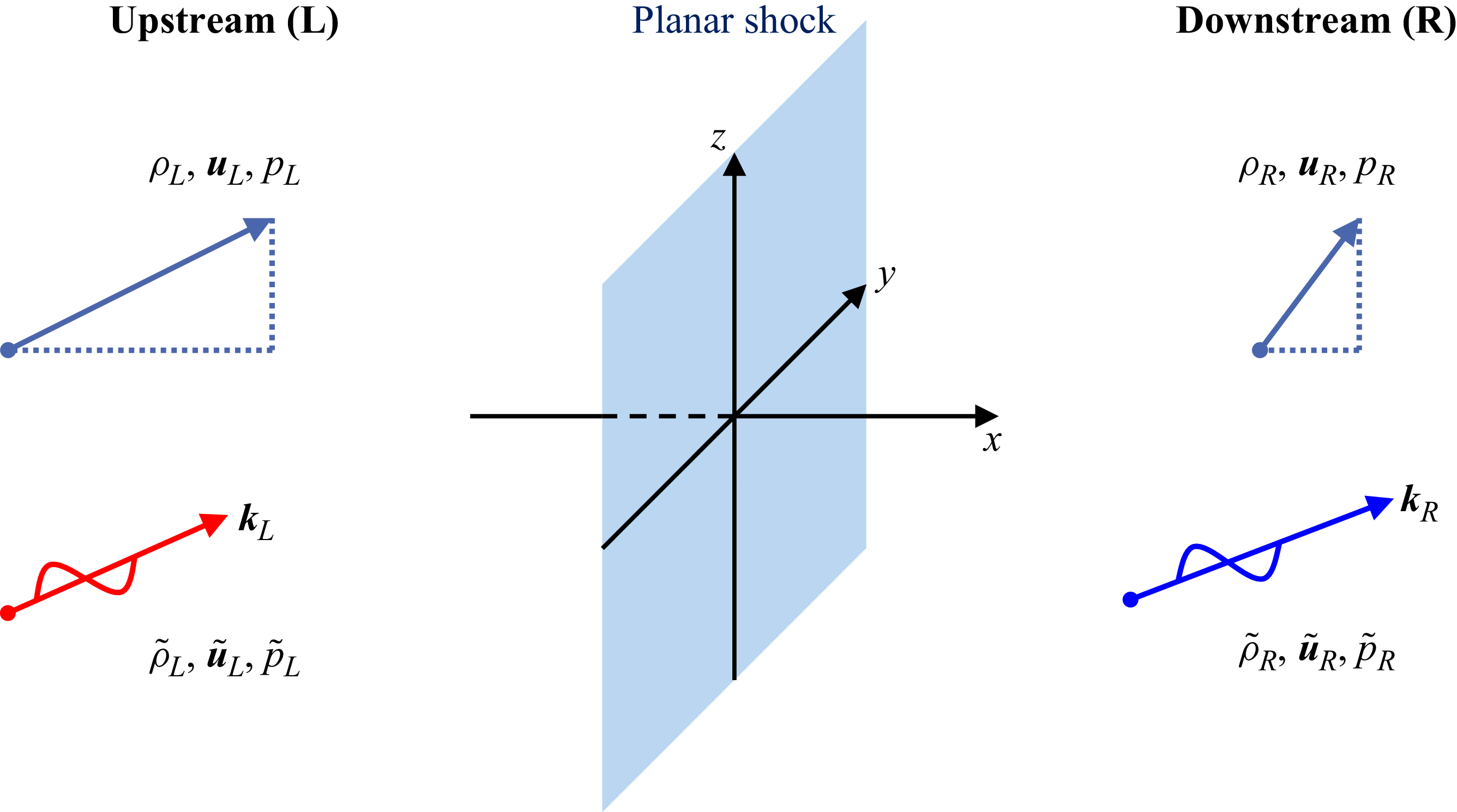
 x
 y
 z

 x=0
 −x
 +x
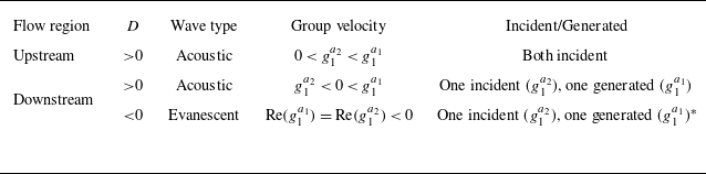
 D
 ∗
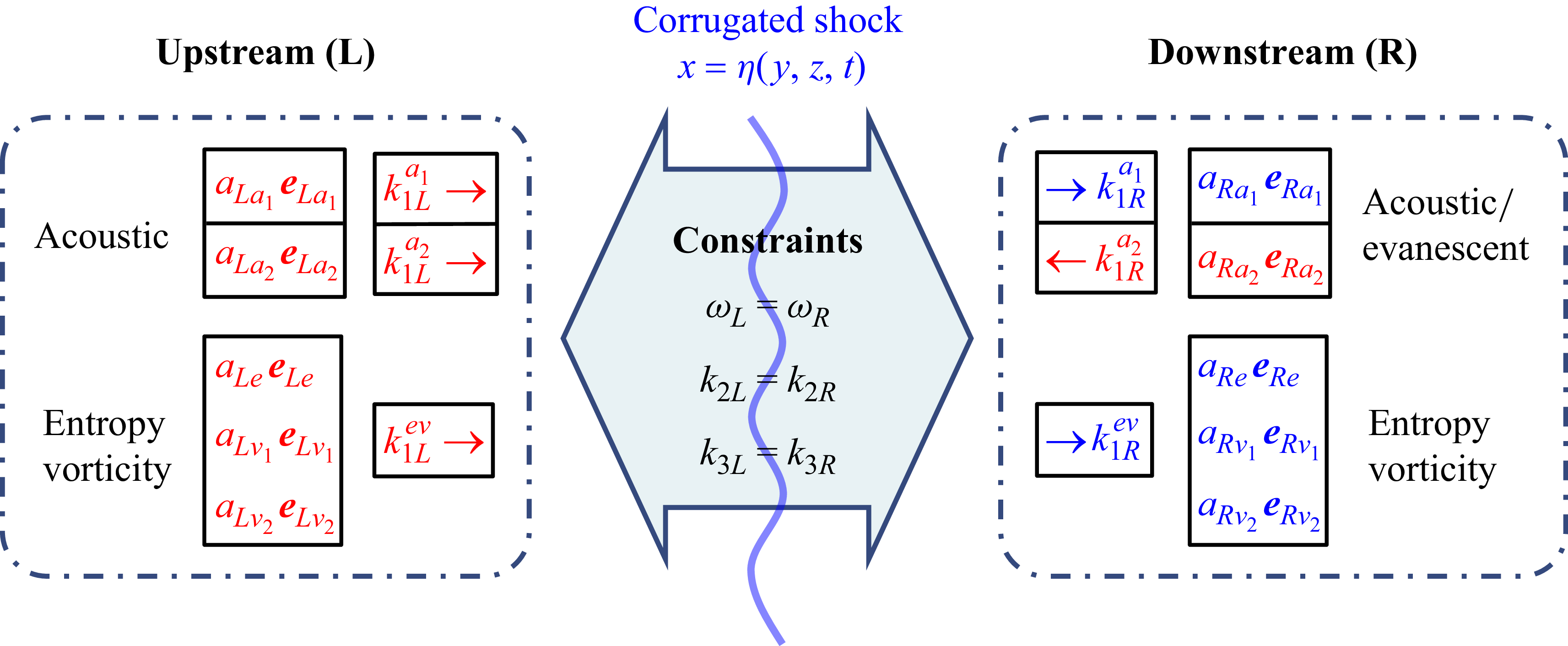
 L
 R
 k2
 k3
 k1
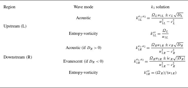
 k1
 (ω,k2,k3)
 Ω=ω−u2k2−u3k3
 D=Ω2+(u12−c2)(k22+k32)
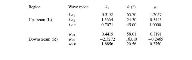
 k1
 θ
 g1
 (ω,k2,k3)=(0.7071,0.7071,0)
 a1
 a2
 ev

 k
 g
 (Ω,k2,k3)=(0.7071,0.7071,0)
 ∝
 c
 u2=0
 u2=−1.25

 θLev
 tanθ=k2/Re(k1R)
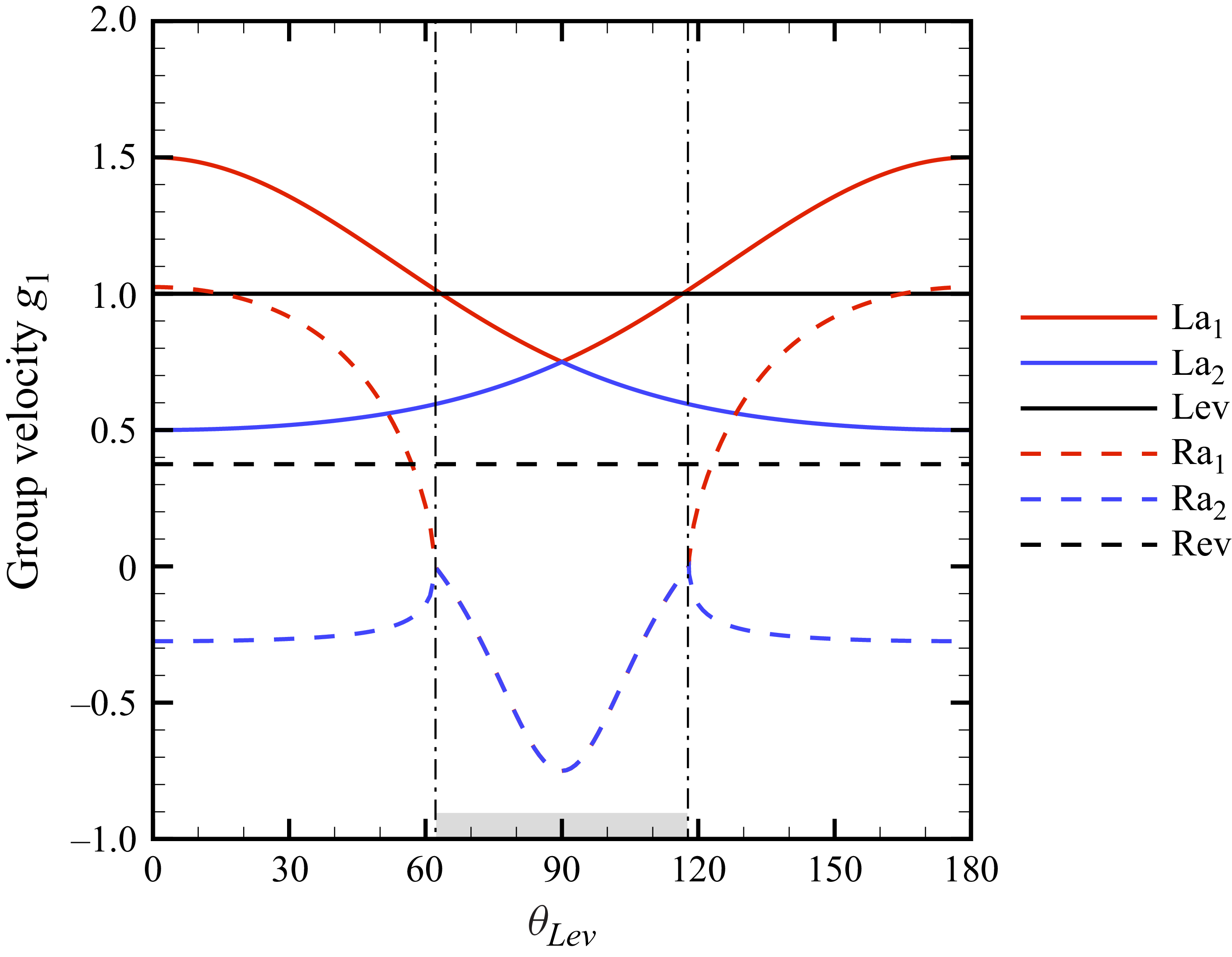
 g1
 θLev
 Re(g1)
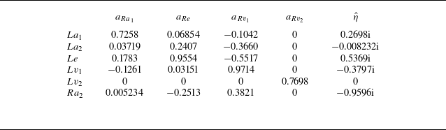
 aRa1
 aRe
 aRv1
 aRv2
 η^
 La1,La2,Le,Lv1,Lv2,Ra2
 (ω,k2,k3)=(0.7071,0.7071,0)

 θLev
 η^
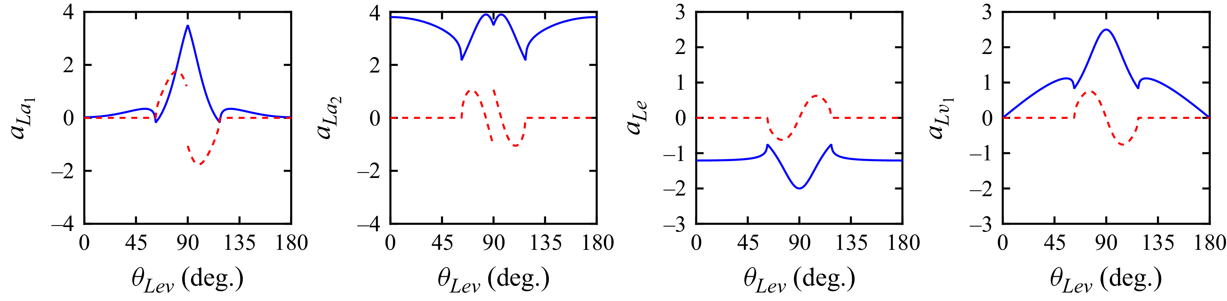
 La1
 La2
 Le
 Lv1
 Ra2
 θLev

 aLa1
 aLa2
 aLe
 aLv1
 θLev
 η^
 aRa2=0

 (ω,k2)=(0.5,1.0)



