TDTR fundamentals

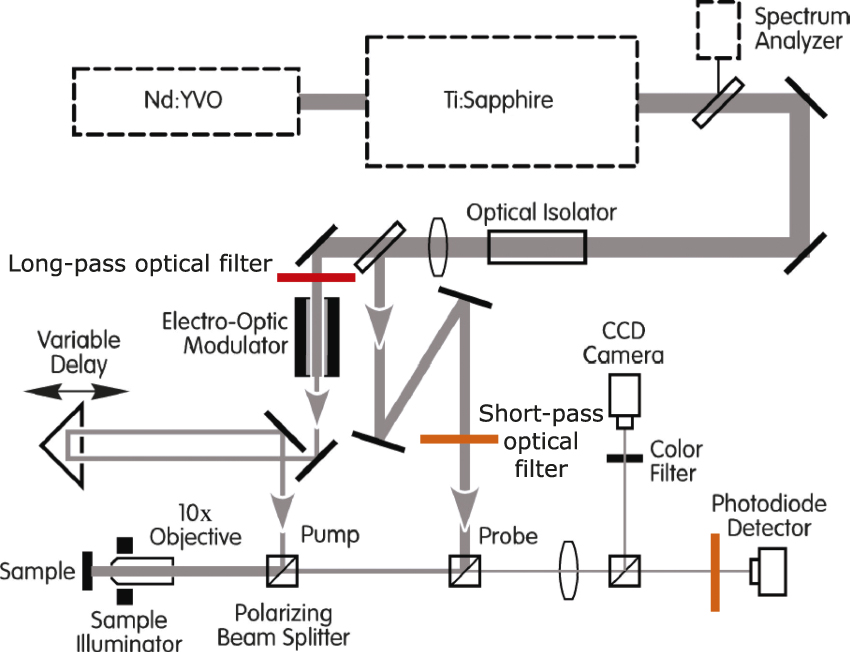
In developing TDTR, in one sense, all we have done is to use modern optical instrumentation to extend the frequency-domain measurements pioneered by Ångström from frequencies on the order of mHz to GHz. The basic layout of a TDTR apparatus is shown in Figure 1 and has not changed significantly since we first assembled the original pump-probe instrument in 2000.^{Reference O’Hara, Hu and Cahill8} The two TDTR systems currently in use at the University of Illinois are based on ultrafast titanium:sapphire laser oscillators, a widely used commercially available laser technology that produces pulses of light that have durations of approximately 200 fs at a rate of 80 MHz. In terms of length scales instead of time scales, each optical pulse is approximately 60-µm long and separated from neighboring pulses by 3.8 m. The pulses of light are split into two paths: one path is the “pump,” which injects heat into the sample, and the second path, the “probe,” which measures the optical response of the sample, and reports back its temperature.

Figure 1.

Schematic diagram of the optical layout of a time-domain thermoreflectance apparatus. In this layout, a “two-tint” approach using sharp-edged optical filters spectrally separates the pump and probe.^{Reference Kang, Koh, Chiritescu, Zheng and Cahill18}

In a conventional TDTR measurement, the reflected probe is incident on a photodiode detector that measures the changes in optical reflectivity of the sample using a lock-in amplifier synchronized to the 10 MHz modulation frequency of the pump. By analyzing this temperature evolution as a function of the delay time between the arrival of the pump and the probe pulses, and also importantly, taking into account the frequency at which the pump beam is modulated and the accumulation of heat created by a sequence of pump pulses, we can accurately determine the thermal-transport properties of the sample.

In a typical experiment, the arrival of the pump pulse at a delay time t = 0 creates a temperature rise of a few degrees K and a change in reflectivity of the metal film transducer on the order of 0.01%. The change in reflectivity decays quickly on picosecond time scales as heat diffuses through the metal transducer and then decays more slowly as heat moves across the metal/sample interface and diffuses into the sample. The noise floor of TDTR measurement is approximately 1 ppm in a 1 Hz bandwidth, or, equivalently, 10 mK in a 1 Hz bandwidth when using Al as the metal film transducer. Therefore, TDTR operates at a high signal-to-noise ratio, and data collection for a single sample can be completed in a few minutes.

An important aspect of the TDTR measurement approach is the collection of picosecond acoustics^{Reference Thomsen, Strait, Vardeny, Maris and Tauc9} data in the same experiment used to measure the thermal signals. The ultrafast temperature excursion created by the pump optical pulse generates a longitudinal acoustic pulse, with a characteristic wavelength on the order of 30 nm, which propagates through the sample, reflects from interfaces, and returns to the surface to produce small changes in the reflectivity. The positions of the echoes can be used to measure film thickness if the sound velocity is known, or they can be used to measure sound velocities if the thickness is known.

History

Ultrafast time-domain measurements of thermal transport were first carried out by the groups of G. Eesley^{Reference Paddock and Eesley10} and H. Maris and colleagues^{Reference Young, Thomsen, Grahn, Maris, Tauc, Anderson and Wolfe11} more than 30 years ago. They used mode-locked dye lasers to study the transport of heat in metal films and the thermal conductance of metal/dielectric interfaces, respectively. Maris’s group published extensively in the 1990s on the thermal conductance of interfaces between materials;^{Reference Stoner and Maris12} they also applied pump-probe methods to measure the thermal conductivity of superlattices.^{Reference Capinski, Maris, Ruf, Cardona, Ploog and Katzer13}

At the University of Illinois, K. O’Hara, a postdoctoral research associate, set up our first TDTR apparatus in 2000.^{Reference O’Hara, Hu and Cahill8} R. Costescu was the first graduate student, in 2003, who compiled measurements of thermal transport by TDTR.^{Reference Costescu, Wall and Cahill14} In 2004, I published an exact solution for analyzing TDTR data.^{Reference Cahill15} Over the subsequent 14 years, we developed thermal conductivity mapping,^{Reference Huxtable, Cahill, Fauconnier, White and Zhao16} discovered frequency-dependent thermal conductivity,^{Reference Koh and Cahill17} and made various tweaks to the experiment to make the measurements more robust.^{Reference Kang, Koh, Chiritescu, Zheng and Cahill18} We also developed data analysis methods to accommodate any form of anisotropy^{Reference Feser and Cahill19,Reference Feser, Liu and Cahill20} and heat conduction by more than one channel of thermal excitations.^{Reference Wilson, Feser, Hohensee and Cahill21} A recent emphasis has been our use of different optical effects beyond thermoreflectance (e.g., plasmonic structures^{Reference Huang, Park, Wang, Murphy and Cahill22} and magneto-optics^{Reference Liu, Choi and Cahill23}) as ultrafast optical thermometers.

Thermal conductivity and interface thermal conductance

The ultimate goal of this measurement machinery is to determine thermal transport coefficients of materials and interfaces. Why is that important? Thermal conductivity goes into the diffusion equation that is then used to model the transport of heat in engineering systems. The ratio of thermal conductivity and heat capacity per unit volume is the thermal diffusivity; the square root of their product is the thermal effusivity. Another key property, particularly at nanometer length scales,^{Reference Kapitza24,Reference Cahill, Braun, Chen, Clarke, Fan, Goodson, Keblinski, King, Mahan, Majumdar, Maris, Phillpot, Pop and Shi25} is the interface thermal conductance, the radiative boundary condition on the heat diffusion equation at the boundary between two materials. The temperature drop across an interface is given by the interface thermal conductance multiplied by the heat flux crossing the interface.

A useful way of thinking about length scales in nanoscale thermal-transport problems is to divide the thermal conductivity by the thermal conductance of an interface. That length is typically referred to as the “Kapitza length” in honor of P.L. Kapitza, Russian scientist and Nobel Laureate who first studied this problem in the context of liquid helium in contact with Cu.^{Reference Kapitza24} The Kapitza length, for a typical interface between Al and diamond and referenced to diamond, is on the order of 10 µm. That means the Al–diamond interface has the same thermal resistance as a 10-µm-thick layer of diamond. At the opposite extreme, the interface between aluminum and a polymer produces a Kapitza length on the order of 1 nm (i.e., the metal–polymer interface adds an extra thermal resistance equivalent to a 1-nm-thick layer of the polymer).

In a typical TDTR experiment, an 80-nm-thick Al coating is used as the metallic transducer. The Al coating generally has to be at least 50-nm thick to adequately block optical signals that come from the material under study. Since the thermal models assume that the optical signals are proportional to the temperature of the Al film, any signals coming from the material under study invalidate the model. To better understand the time scales of a TDTR experiment, consider the time required for heat to diffuse a distance of 50 nm. In diamond, that time scale is extremely fast, about 25 ps; in a polymer, that time scale is three orders of magnitude longer. Therefore, the experiment has to span a wide range of time scales for it to be applicable to a wide range of materials. If we also consider the thermal conductance of the metal–sample interfaces, the characteristic thermal time scale of the metal layer is typically greater than 1 ns. The important consequence of this is that the time-domain signal (i.e., the decay of the temperature of the transducer measured on time scales up to a few nanoseconds) has very limited sensitivity to the properties of the material that we want to study. To study the material properties, we have to access much longer time scales, tens of nanoseconds, and that comes from modulation of the pump at MHz frequencies.

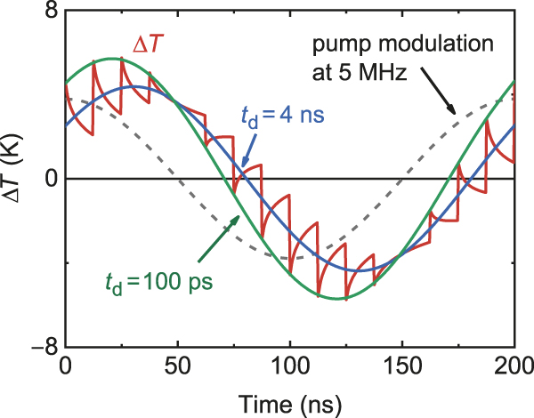
Figure 2 illustrates the experiment as a function of time. The pump modulation frequency in this example is 5 MHz. At each point in time that a pump pulse arrives at the sample, the pump pulse produces a temperature excursion in the sample, which then decays. In this calculation, each pump pulse produces some amount of heating in the first half of the cycle and some amount of cooling in the second half of the cycle because this calculation uses the fundamental harmonic of the modulation frequency and we have omitted the DC component of the heating by the pump. The temperature oscillations can be described by an amplitude and a phase, or more conveniently in most cases, a real and imaginary component. We measure the real and imaginary parts of the temperature oscillations at the pump modulation frequency as a function of the pump-probe delay time^{Reference Cahill15} using lock-in detection.

Figure 2.

Calculations of the temperature response of the surface of a sample in a thermoreflectance experiment. The sample geometry is 80-nm Al deposited on 500-nm-thick a-SiO₂ layer on Si. The repetition rate of the laser is 80 MHz and the modulation frequency of the pump beam is 5 MHz. This calculation only considers the fundamental Fourier component of the modulation frequency. The temperature response is labeled for two delay times, t _d = 100 ps and 4 ns.

The key innovation of TDTR as implemented at the University of Illinois in the early 2000s is making use of both the time-domain and frequency-domain response. While the full equations are too complicated to discuss here and are presented elsewhere,^{Reference Cahill15} we illustrate the basic idea approximately considering what the in-phase time-domain signal measures at short delay times, and how the out-of-phase signal depends on the frequency-domain response. The temperature jump near t = 0 in the in-phase or real component of the response is inversely proportional to the heat capacity per unit area of the metal film transducer. The out-of-phase or imaginary component of the response that comes out of the analysis of the measurement is, to first approximation, determined by the reciprocal of the effusivity, the square root of the product of the heat capacity and thermal conductivity.^{Reference Cahill15} The ratio of these two quantities (the in-phase temperature jump divided by the out-of-phase signal), is proportional to the square root of the thermal conductivity and is independent of the laser power and thermoreflectance coefficient, dR/dT, where R is the optical reflectivity. This square root dependence of the ratio signal is sufficient to produce good sensitivity to the thermal conductivity across the whole range of thermal conductivities of materials (0.05–2000 W m^–1 K^–1) near room temperature.^{Reference Cahill, Braun, Chen, Clarke, Fan, Goodson, Keblinski, King, Mahan, Majumdar, Maris, Phillpot, Pop and Shi25}

High thermal conductivity in cubic BAs

An example of an application of TDTR is the search for new materials with high thermal conductivity. In 2013, D. Broido, L. Lindsay, and T. Reinecke theoretically predicted high thermal conductivities in crystals of boron arsenide, boron nitride, boron phosphide, and boron antimony with the zinc-blende structure.^{Reference Lindsay, Broido and Reinecke26} An unexpected and exciting result was that BAs was predicted to have a thermal conductivity comparable to that of diamond. This remarkable behavior has to do with details of the phonon dispersion and the large gap between the highest frequency of the acoustic modes and the lowest frequency of the optical modes.

As experimentalists, our task is to see if such crystals can be made and see if they have the thermal conductivity that is predicted. It should be noted, however, that the original theoretical prediction was based on the approximation that phonon scattering is adequately accounted for by, and including, terms up to the third order. It turns out that for BAs, fourth-order terms in the scattering of phonons become important because of the weakness of the three-phonon scattering.^{Reference Feng, Lindsay and Ruan27} The theoretical predictions since 2013 have dropped by approximately a factor of two with the inclusion of fourth-order processes.

With TDTR, we can now routinely measure the thermal conductivity of specimens with dimensions below 100 μm. Figure 3a shows a scanning electron microscope image of a BAs crystal; Figure 3b is an optical micrograph taken in the TDTR apparatus. The optical image shows the position of the pump laser beam on a growth facet of one of the BAs crystals after the crystal was coated with an 80-nm-thick film of Al.

Figure 3.

(a) Scanning electron microscope image of a BAs crystal grown by a chemical-vapor-transport method.^{Reference Li, Zheng, Lv, Liu, Wang, Huang, Cahill and Lv1} (b) Dark-field optical microscope image of an Al-coated BAs crystal collected by the camera in the time-domain thermoreflectance system. The bright spot near the bottom is the pump laser spot with 1/e^{Reference Xie, Li, Tsai, Liu, Braun and Cahill2} intensity radius of 11 μm. (c) Thermal conductivity of four BAs crystals and comparisons to the theoretical calculations in References Reference Lindsay, Broido and Reinecke26 and Reference Feng, Lindsay and Ruan27. Roman numerals indicate sample numbers. The curve labeled “3ph” is a calculation limited to three-phonon scattering. The curve labeled “3ph + 4ph” refers to a calculation that considers both three-phonon and four-phonon scattering.^{Reference Li, Zheng, Lv, Liu, Wang, Huang, Cahill and Lv1}

We now have relatively complete sets of TDTR thermal conductivity data over a wide range of temperatures for BP, BAs, GaN, and SiC. The data for BAs were reported in a recent publication.^{Reference Li, Zheng, Lv, Liu, Wang, Huang, Cahill and Lv1} Figure 3c compares data for the highest thermal conductivity crystal of BAs we have studied to date to theoretical predictions. Similar data were obtained independently by two other groups and also published at the same time.^{Reference Kang, Li, Wu, Nguyen and Hu28,Reference Tian, Song, Chen, Ravichandran, Lv, Chen, Sullivan, Kim, Zhou, Liu, Goni, Ding, Sun, Gamage, Sun, Ziyaee, Huyan, Deng, Zhou, Schmidt, Chen, Chu, Huang, Broido, Shi, Chen and Ren29}

The room-temperature thermal conductivity of isotopically enriched BP is approximately 500 W m^–1 K^–1. Similar data, also acquired with TDTR, were recently reported.^{Reference Kang, Wu and Hu30} The thermal penetration depth, $L = \sqrt {D/(\pi f)}$, where D is the thermal diffusivity and f is the modulation frequency of the pump beam, is an important length scale in a TDTR measurement. Phonons are the dominant heat-carrying excitation in dielectric and semiconducting crystals. The distribution of the mean free paths of phonons in crystals that are important for heat conduction is broad, typically spanning two orders of magnitude, but consider an approximation where all phonons have the same mean free path, $\ell = v\tau$. The diffusivity then is $D = v\ell /3$ and $L = \ell \sqrt {1/(3\pi f\tau )}$. Since $f\tau \ll 1$, $L \gg l$, we do not have to be concerned about the effects of ballistic (nondiffusive) phonon transport on the TDTR measurement. In reality, the phonon mean free path distribution is indeed broad; for some fraction of the heat-carrying phonons, $L < l$, and the TDTR measurements can be affected by deviations from diffusive transport.^{Reference Wilson and Cahill31} Near room temperature and above, these are usually small effects and, furthermore, we can check the importance of nondiffusive transport by examining how the thermal conductivity derived from a TDTR measurement varies with the size of the laser spots. So-called “deviations from Fourier’s Law” in crystals are a topic of great current interest in the materials physics of the conduction of heat by phonons.^{Reference Wilson and Cahill31,Reference Hua and Minnich32}

Thermal conductivity of amorphous polymers

An important aspect of the TDTR measurement approach is that we can easily quantify the sensitivity of the data to variations in the fixed and free parameters. This “sensitivity analysis” allows us to optimize the design of experiments (i.e., the choice of spot size, transducer material, layer thicknesses, and substrate material) and understand the propagation of systematic errors. A convenient definition of the sensitivity is the logarithmic derivative of the TDTR ratio signal $\varphi$ taken with respect to one of the parameters in the thermal model while holding all other parameters fixed. For example, the sensitivity to interface thermal conductance S _G is ${S_G} = d\ln \varphi /d\ln G$. In this example, if, for small changes in the interface conductance G, $\varphi$ scales with a power law G ^α, then S _G = α.

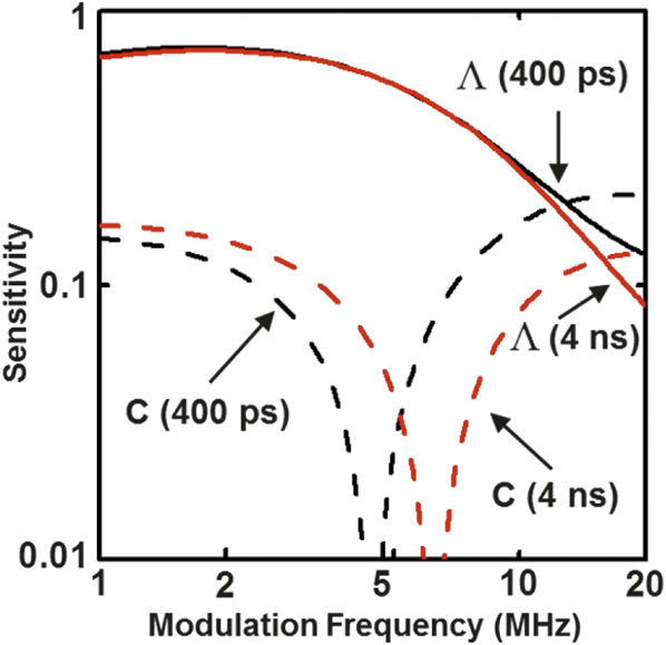
In our study of the thermal conductivity Λ and heat capacity C of fullerene derivatives^{Reference Wang, Liman, Treat, Chabinyc and Cahill33} and amorphous polymers,^{Reference Xie, Li, Tsai, Liu, Braun and Cahill2,Reference Xie, Yang, Li, Tsai, Shin, Braun and Cahill3} we took advantage of how the sensitivities vary with film thickness and modulation frequency and designed experiments that could determine both Λ and C. Figure 4 shows calculations of the sensitivities. Typically, we use a modulation frequency of 10 MHz in TDTR measurements and at those frequencies, the sensitivity to both Λ and C is approximately 0.25. At intermediate modulation frequencies, the sensitivity to C passes through zero and at low modulation frequency, the sensitivity to Λ is enhanced while the sensitivity to C is still small. By combining measurements at different frequencies, we can extract both Λ and C of thin polymer films.

Figure 4.

Absolute value of the sensitivity with respect to the thermal conductivity (solid lines) and heat capacity (dashed lines) of a typical polymer film as a function of modulation frequency and delay time between pump and probe (black lines are t = 400 ps, red lines are t = 4 ns). The sensitivities are calculated for a 100-nm polymer film sandwiched between a 90-nm Al transducer and a Si substrate.^{Reference Xie, Li, Tsai, Liu, Braun and Cahill2}

We reported the thermal conductivity, heat capacity, and elastic constants of 27 different polymer structures to explore the structure–property relationship in this class of materials.^{Reference Xie, Li, Tsai, Liu, Braun and Cahill2,Reference Xie, Yang, Li, Tsai, Shin, Braun and Cahill3} Both extremes of high and low thermal conductivity are scientifically interesting and potentially useful to extend. Fully transparent, easily processed polymers that have thermal conductivities above 1 W m^–1 K^–1 might find application in thermal management of photonic devices or for improving the properties of electrical insulation of motors and generators. We need to find inexpensive materials that have thermal conductivities less than polystyrene. Polystyrene and polyurethane foams are widely used in thermal insulation of buildings and refrigeration systems. Could we find ways to reduce heat conduction in the solid material components of such foams and make a technologically significant improvement in their performance?

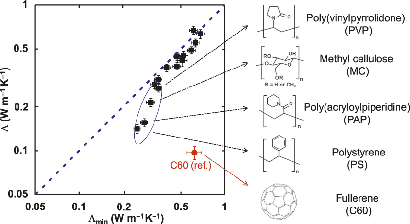
For the most part, the thermal conductivity of amorphous polymers is well correlated with the sound velocities (i.e., the thermal conductivity of amorphous polymers is adequately described by the model of the minimum thermal conductivity).^{Reference Xie, Li, Tsai, Liu, Braun and Cahill2,Reference Xie, Yang, Li, Tsai, Shin, Braun and Cahill3,Reference Hsieh, Losego, Braun, Shenogin, Keblinski and Cahill34} An example of this behavior is shown in Figure 5. The minimum thermal conductivity is calculated from the average speeds of sound and the molecular density. Interestingly, the measured thermal conductivity of polystyrene falls significantly below the prediction of the model. The more dramatic outliers are fullerene derivatives with thermal conductivities a factor of 2–3 smaller than predicted by the model. Fullerene derivatives are, in fact, among the lowest thermal conductivity dense materials ever studied.^{Reference Wang, Liman, Treat, Chabinyc and Cahill33}

Figure 5.

Comparison between the measured thermal conductivity and the predicted value based on the model of the minimum thermal conductivity for a variety of polymer structures.^{Reference Xie, Li, Tsai, Liu, Braun and Cahill2,Reference Xie, Yang, Li, Tsai, Shin, Braun and Cahill3,Reference Wang, Liman, Treat, Chabinyc and Cahill33}

Thermal switching in liquid-crystal networks

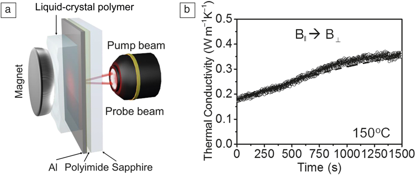
As a final example, we highlight the usefulness of TDTR for measurements of thermal conductivity in real time, following the evolution of materials as a function of environment or processing conditions. We start with a liquid-crystal monomer, which is then cross-linked by photopolymerization to form a liquid-crystal polymer network.^{Reference Shin, Kang, Tsai, Leal, Braun and Cahill4} The liquid-crystal network is coated onto a special test structure of an Al transducer deposited on a thermal insulation layer (typically 100-nm-thick polyimide) on a high thermal conductivity transparent substrate (typically sapphire).

The experimental geometry is illustrated in Figure 6a. The thermal conductivity of the liquid-crystal network depends on the direction of a magnetic field applied to the sample during polymerization. The thermal conductivity is 50% higher when the field direction is normal to the surface and therefore parallel to the direction of heat flow. These studies of thermal conductivity by TDTR were supported by extensive measurements of the molecular structure and ordering using small-angle and wide-angle x-ray scattering performed at the Advanced Photon Source.

Figure 6.

(a) Schematic illustration of time-domain thermoreflectance measurement of a liquid-crystal-network/Al/polyimide/sapphire sample in a magnetic field. (b) Thermal conductivity of a parallel aligned (B_||) liquid-crystal network in response to an orthogonal magnetic field (B_⊥) at 150°C. The magnetic field was switched to the perpendicular direction (B_⊥) at 150°C at t = 0 s.^{Reference Shin, Kang, Tsai, Leal, Braun and Cahill4}

If we then take material that has been aligned by polymerization in a magnetic field and then remove the magnetic field and increase the temperature, the molecular order is lost and the thermal conductivity decreases. With cooling, the thermal conductivity partially recovers. The response of the molecular order to changing temperature or magnetic field orientation can also be monitored in real time using TDTR. Figure 6b displays our study of how the liquid-crystal network responds to a change in the orientation of the magnetic field at fixed temperature as a function of time. This is an example of a material that can be reversibly switched or modulated by an external stimulus.^{Reference Wehmeyer, Yabuki, Monachon, Wu and Dames5}