



1. Introduction
The problem of health and disease has long been a central concern globally. Throughout human history, large-scale outbreaks of infectious diseases such as bubonic plague, smallpox, cholera, influenza, and malaria have inflicted severe, and often devastating, impacts on national economies and people’s livelihoods worldwide (Brauer et al. [Reference Brauer, Castillo-Chavez and Feng5]).
The study of infectious diseases through mathematical modelling has a rich history, dating back to Bernoulli’s [Reference Bernoulli3] work on smallpox vaccination in 1760. In 1906, Hamer [Reference Hamer19] introduced a discrete mathematical model to investigate recurrent measles epidemics. Ross [Reference Ross36] employed a differential equation model in 1911 to analyse the transmission dynamics of malaria between mosquitoes and humans. A major milestone came in 1927, when Kermack and McKendrick [Reference Kermack and McKendrick22] proposed the compartmental model during their study of the Black Death in London and plague outbreaks in Bombay. This laid the foundation for the rapid development of mathematical modelling and dynamical analysis of infectious diseases. A landmark publication was Bailey’s [Reference Bailey2] book in 1957, which became the first comprehensive treatise on the mathematical theory of infectious diseases and its applications.
In recent years, there has been a broad consensus that spatial diffusion and environmental heterogeneity play crucial roles in the transmission dynamics of infectious diseases (Brauer et al. [Reference Brauer, Allen, Van den Driessche and Wu4]). To better understand these effects, Allen et al. [Reference Allen, Bolker, Lou and Nevai1] proposed the following susceptible-infectious-susceptible (SIS) epidemic model
 \begin{equation}
\begin{cases}u_t-d_u \Delta u=-p(x) \frac{u v}{u+v}+q(x) v, & ( x, t) \in \Omega\times\mathbb{R}^{+},
\\ v_t -d_v \Delta v=p(x) \frac{uv}{u+v}-q(x) v, & ( x, t) \in \Omega\times\mathbb{R}^{+}, \\
\frac{\partial u}{\partial \nu}=\frac{\partial v}{\partial \nu}=0, & ( x, t) \in \partial\Omega\times\mathbb{R}^{+}, \\ u(x, 0)=u_0(x), v(x, 0)=v_0(x), & x \in \Omega,
\end{cases}
\end{equation}
where 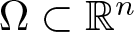 $\Omega\subset\mathbb{R}^{n}$ (
 $n\geq1$) is a bounded domain with smooth boundary;
 $\nu$ denotes the outward unit normal vector
 $\partial\Omega$;
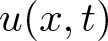 $u(x,t)$ and
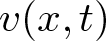 $v(x,t)$ represent the densities of susceptible and infected individuals, respectively, at location
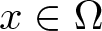 $ x\in\Omega$ and time
 $t$. The positive constants
 $d_u$ and
 $d_v$ are the diffusion rates for susceptible and infected populations, while
 $p(x)$ and
 $q(x)$ are positive Hölder continuous functions on
 $\Omega$ that denote the spatial-dependent disease transmission and recovery rates, respectively. Using a variational characterization, the authors defined the basic reproduction number and established it as a threshold for the stability of the disease-free equilibrium (DFE) and the existence of an endemic equilibrium (EE). Subsequently, Peng [Reference Peng32] investigated the asymptotic behaviour of the EE of system (1.1) and demonstrated that restricting the movement of susceptible individuals is an effective strategy for disease elimination. Peng and Liu [Reference Peng and Liu31] further analysed the global asymptotic stability of both the DFE and EE of system (1.1). In 2013, Peng and Yi [Reference Peng and Yi33] extended the model to a more complex heterogeneous environment incorporating high-, medium-, and low-risk areas, and examined the asymptotic profiles of the EE of system (1.1) across these regions. Their work highlights how spatial disease risk and population mobility shape the distribution of infectious diseases. For more research related to system (1.1), we refer readers to Cui et al. [Reference Cui, Li, Peng and Zhou11], Deng and Wu [Reference Deng and Wu12], Gao et al. [Reference Gao, Lei, Peng and Zhang15], Ge et al. [Reference Ge, Kim, Lin and Zhu16], Hu et al. [Reference Hu, Jin and Wang21], Li et al.[Reference Li, Peng and Wang23], Li and Xiang [Reference Li and Xiang24], Wu and Zou [Reference Wu and Zou43], and the references therein.
Seasonal variations in environmental factors, such as rainfall, temperature, humidity, and air pollution, are ubiquitous in nature and exert a profound influence on human life and the spread of infectious diseases (Cantrell and Cosner [Reference Cantrell and Cosner8], Wang and Zhao [Reference Wang and Zhao40]). Therefore, accounting for the periodic nature of these seasonal variations is essential for understanding temporal heterogeneity in disease dynamics. Reflecting this perspective, Peng and Zhao [Reference Peng and Zhao34] proposed the following reaction-diffusion SIS epidemic model within a time-periodic environment
 \begin{equation}
\begin{cases}u_t-d_u \Delta u=-p(x,t) \frac{u v}{u+v}+q(x,t) v, & ( x, t) \in \Omega\times\mathbb{R}^{+},
\\ v_t -d_v \Delta v=p(x,t) \frac{uv}{u+v}-q(x,t) v, & ( x, t) \in \Omega\times\mathbb{R}^{+}, \\
\frac{\partial u}{\partial \nu}=\frac{\partial v}{\partial \nu}=0, & ( x, t) \in \partial\Omega\times\mathbb{R}^{+}, \\ u(x, 0)=u_0(x), v(x, 0)=v_0(x), & x \in \Omega,
\end{cases}
\end{equation}
where  $p(x,t)$ and
 $q(x,t)$ represent the disease transmission and recovery rates, respectively, at location
 $x$ and time
 $t$. They defined the basic reproduction number using the next infection operator method and investigated the long-term behaviour of solutions to system (1.2). For further background on the next infection operator, we refer to Van den Driessche and Watmough [Reference Van den Driessche and Watmough39] and Wang and Zhao [Reference Wang and Zhao42], among other references. Their analysis revealed a key insight: both spatial heterogeneity and temporal periodicity can enhance disease persistence (Peng and Zhao [Reference Peng and Zhao34]). More recently, Liu and Lou [Reference Liu and Lou26] studied the asymptotic behaviour of endemic periodic solutions of system (1.2) and emphasized that restricting the movement of susceptible populations may serve as an effective measure for disease control.
In systems (1.1)–(1.2), the diffusion process is modelled using the Laplace operator, which corresponds to localized Brownian random motion. However, recent studies indicate that human mobility patterns exhibit scale-free, nonlocal dynamics with heavy-tailed distributions characteristic of Lévy flights (Mandelbrot [Reference Mandelbrot29] and Zaburdaev et al. [Reference Zaburdaev, Denisov and Klafter45]). Empirical analyses of banknote circulation, mobile phone data, and hunter-gatherer movement have revealed that human trajectories are better described by Lévy flights, nonlocal stochastic processes with long-tailed probability distributions, rather than by local random motion (Brockmann et al. [Reference Brockmann, Hufnagel and Geisel6]; González et al. [Reference González, Hidalgo and Barabási17]; Raichlen et al. [Reference Raichlen, Wood, Gordon, Mabulla, Marlowe and Pontzer35]). It has been shown that the Lévy diffusion can be effectively modelled using the spectral fractional Laplace operator  $\left(-\Delta_N\right)^{s}$ (the exact definition will be given soon), where
 $0 \lt s \lt 1$ (Chaves [Reference Chaves9]). Most applications of this operator have focused on individual equations, such as the Fisher–KPP (Kolmogorov, Petrovskii, Piskunov) equation and the Allen–Cahn equation (see Gui and Zhao [Reference Gui and Zhao18], Ma et al. [Reference Ma, Niu and Wang28], Stan and Vázquez [Reference Stan and Vázquez38], and the cited references therein). The introduction of Lévy flight diffusion is considered a significant advancement in modelling infectious disease transmission (Brockmann et al. [Reference Brockmann, Hufnagel and Geisel6]), as fractional diffusion effectively captures long-range dispersal dynamics (Hanert et al. [Reference Hanert, Schumacher and Deleersnijder20]). Recently, Zhao and Ruan [Reference Zhao and Ruan46] proposed the following SIS epidemic model with fractional diffusion
 \begin{equation}
\begin{cases}u_t+\left(-d_u \Delta_N\right)^{s_1} u=a(x) u-b(x) u^2-p(x)\frac{u v}{u+v}+q(x) v, & ( x, t) \in \overline{\Omega}\times\mathbb{R}^{+}, \\
v_t+\left(-d_v \Delta_N\right)^{s_2} v=p(x)\frac{u v}{u+v}-q(x) v, & ( x, t) \in \overline{\Omega}\times\mathbb{R}^{+}, \\
u(x,0)=u_0(x), v(x,0)=v_0(x), & x \in \overline{\Omega}, \end{cases}
\end{equation}
where  $0 \lt s_1, s_2 \lt 1$ denote the fractional powers of
 $- \Delta_N$, which is the Neumann realization of
 $-\Delta$ in a suitable function space,
 $(-\Delta_N)^s(s=s_1\ \text{or}\ s_2)$ is the spectral fractional Neumann Laplace operator and defined by
 \begin{equation*}
\left(-\Delta_N\right)^s w=\sum_{m=1}^{\infty} \lambda_m^s w_m \psi_m=\frac{1}{\Gamma(-s)} \int_0^{\infty} \frac{e^{\Delta_N t} w-w}{t^{1+s}} d t,
\end{equation*}
where  $\left(\lambda_m, \psi_m\right)_{m=1}^{\infty}$ are eigen-pairs of
 $-\Delta_N$,
 $w(x)=$
 $\sum_{m=1}^{\infty} w_m \psi_m(x)$ and
 $w_m=\left\langle w, \psi_m\right\rangle$ (
 $\langle\cdot, \cdot\rangle$ is the inner product in
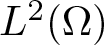 $L^2(\Omega)$),
 $\Gamma$ is the Gamma function and
 $e^{\Delta_N t}$ is the semigroup generated by
 $\Delta_N$, the
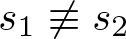 $s_1 \not\equiv s_2$ here conforms to the spreading behaviour that is not completely the same between susceptible and infected populations. They investigated the existence and stability of disease-free and endemic equilibria and analysed the influence of diffusion coefficients and fractional powers on the asymptotic behaviour of equilibrium solutions. For further research on epidemic models with nonlocal diffusion, we refer to Feng et al. [Reference Feng, Li, Ruan and Yang13], Feng et al. [Reference Feng, Li and Yang14], Lin and Wang [Reference Lin and Wang25], Shi et al. [Reference Shi, Li and Yang37], Yang et al. [Reference Yang, Li and Ruan44], and the references therein.
In this paper, we propose the following SIS epidemic model with fractional diffusion and spatio-temporal heterogeneity
 \begin{equation}
\begin{cases}u_t+\left(- d_u\Delta_N\right)^{s_1} u= -\frac{p(x,t) u v}{u+v}+q(x,t) v, & ( x, t) \in \overline{\Omega}\times\mathbb{R}^{+}, \\
v_t+ \left(-d_v\Delta_N\right)^{s_2} v=\frac{p(x,t)u v}{u+v}-q(x,t) v, & ( x, t) \in \overline{\Omega}\times\mathbb{R}^{+}, \\
u(x,0)=u_0(x), v(x,0)=v_0(x), & x \in \overline{\Omega}, \end{cases}
\end{equation}
where the parameters retain the same meanings as in systems (1.1)–(1.3). Throughout this paper, we impose the following assumptions:
(H1)  $\int_\Omega v(x,0)dx \gt 0$,
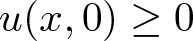 $u(x,0)\geq0$ and
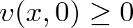 $v(x,0)\geq0$ are continuous on
 $\overline{\Omega} $;
(H2)  $\int_\Omega (u(x,0)+v(x,0))dx\equiv N \gt 0$, where
 $N$ denotes the total population number;
(H3) 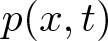 $p(x,t)$,
 $q(x,t)$ are positive and Hölder continuous on
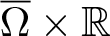 $\overline{\Omega}\times\mathbb{R}$, and are
 $T$-periodic in time, i.e.,
 $p(x,t)=p(x,t+T)$ and
 $q(x,t)=q(x,t+T)$ for all
 $(x,t)\in\overline{\Omega}\times\mathbb{R}$, with
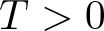 $T \gt 0$.
Demographic processes such as births and deaths may be neglected when the disease dynamics occur on a much faster time scale (Brauer et al. [Reference Brauer, Castillo-Chavez and Feng5]). Our assumption (H2) reflects this premise. We now define the Sobolev–Slobodeckii space 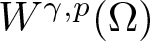 $W^{\gamma,p}(\Omega) $ as follows
 \begin{equation*}
\begin{aligned}
W^{\gamma,p}(\Omega)=\left\{\partial^{|\beta|} w \in L^p(\Omega), 0 \leq|\beta| \leq[\gamma] \Big|
[w]_{W^{\gamma,p}(\Omega)}^p \lt \infty \right\},
\end{aligned}
\end{equation*}
where the seminorm is given by
 \begin{equation*}
[w]_{W^{\gamma,p}(\Omega)}^p:=\sum_{|\beta|=0}^{[\gamma]} \int_{\Omega} \int_{\Omega} \frac{|\partial^{|\beta|} w(x)-\partial^{|\beta|} w(y) |^p}{|x-y|^{n+ sp}} d y d x,
\end{equation*}
with  $\gamma \in \mathbb{R}^{+} \setminus \mathbb{N}$,
 $s = \gamma - [\gamma]$,
 $[\gamma]$ the integer part of
 $\gamma$, and
 $1 \lt p \lt \infty$. We denote
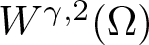 $W^{\gamma,2}(\Omega)$ by
 $H^\gamma(\Omega)$. As established in Zhao and Ruan [Reference Zhao and Ruan46], the bilinear form
 $\left\langle\left(-\Delta_N\right)^s \cdot \mid \cdot\right\rangle: H^s(\Omega) \times H^s(\Omega) \rightarrow \mathbb{R}$ associated with
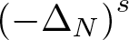 $\left(-\Delta_N\right)^s$ is defined by
 \begin{equation}
\left\langle\left(-\Delta_N\right)^s u \mid v\right\rangle=\int_{\Omega} \int_{\Omega} K_{s}(x, y)[u(x)-u(y)][v(x)-v(y)] d y d x,~ u,v\in H^s(\Omega),
\end{equation}
where
 \begin{equation*}
K_{s}(x, y)=\frac{1}{2|\Gamma(-s)|} \int_0^{\infty} \frac{G_N(t, x, y)}{t^{1+s}} d t
\end{equation*}
is a symmetric kernel satisfying the two-sided Gaussian estimate
 \begin{equation}
\frac{C_1}{|x-y|^{n+2 s}} \leq K_{s}(x, y) \leq \frac{C_2}{|x-y|^{n+2 s}},~x,~y\in\Omega,~x \neq y,
\end{equation}
and the constants  $C_1, C_2 \gt 0$ depending on
 $s$ and
 $\Omega$. Here,
 $G_N$ denotes the heat kernel associated with the semigroup
 $e^{\Delta_N t}$ for
 $t \gt 0$. For further details on fractional Laplace operators, we refer to Caffarelli and Stinga [Reference Caffarelli and Stinga7].
The primary objective of this paper is to investigate how spatio-temporal heterogeneity and fractional diffusion influence the extinction and persistence of infectious diseases, and to establish a theoretical foundation for informing public health policies and interventions. It is noteworthy that Zhao and Ruan [Reference Zhao and Ruan46] focused on the autonomous system (1.3), that is,  $p(x, t) \equiv p(x)$ and
 $q(x, t) \equiv q(x)$. In that setting, the basic reproduction number
 $\mathcal{R}_0$ admits a variational formulation, which facilitates the analysis of its monotonicity and asymptotic behaviour with respect to the diffusion rate. In contrast, this paper deals with the nonautonomous system (1.4), where
 $\mathcal{R}_0$ lacks a variational structure, thereby complicating the study of its monotonicity and asymptotic properties. To address this challenge, we employ next-generation operator theory to define
 $\mathcal{R}_0$, and subsequently reveal the following key properties: first,
 $\mathcal{R}_0$ is always independent of the diffusion rate
 $d_u$ of the susceptible population; second,
 $\mathcal{R}_0$ is independent of
 $d_v$ when
 $p$ and
 $q$ are temporally heterogeneous (i.e.,
 $p(x, t) \equiv p(t)$,
 $q(x, t) \equiv q(t)$); third,
 $\mathcal{R}_0$ is a non-increasing function of
 $d_v$ when
 $p$ and
 $q$ are spatially heterogeneous (i.e.,
 $p(x, t) \equiv p(x)$,
 $q(x, t) \equiv q(x)$); and finally, under general spatio-temporal heterogeneity,
 $\mathcal{R}_0$ is generally not monotonous about
 $d_v$.
Furthermore, we establish general conditions for the existence and uniqueness of global solutions to system (1.4), as well as its point dissipativity. Inspired by the ideas of Peng and Zhao [Reference Peng and Zhao34], using the theory of uniform persistence, we demonstrate the existence of periodic solutions and analyse the long-term behaviour of global solutions to system (1.4). On this basis, we further investigate how variations in the diffusion rate parameters affect the asymptotic behaviour of periodic solutions. In addition, we provide a general criterion for the uniqueness of periodic solutions.
The main contributions of this study are as follows: i) extending the work of Zhao and Ruan [Reference Zhao and Ruan46] to a more general case where  $p$ and
 $q$ exhibit spatio-temporal heterogeneity; ii) establishing a universal criterion for the existence and uniqueness of equilibrium solutions, a topic not addressed in previous studies such as Peng and Zhao [Reference Peng and Zhao34] and Zhao and Ruan [Reference Zhao and Ruan46]. Finally, we emphasize that spatio-temporal heterogeneity can significantly facilitate the sustained transmission of infectious diseases.
The remainder of this paper is organized as follows. In Section 2, we introduce the basic reproduction number  $\mathcal{R}_0$ and establish threshold dynamics for disease extinction and persistence based on
 $\mathcal{R}_0$. Section 3 is devoted to the analysis of the asymptotic profiles of endemic periodic solutions of system (1.4). In Section 4, we summarize the conclusions of the paper, propose several effective measures for controlling the spread of infectious diseases, and suggest some directions for future research.
2. Existence and stability of disease-free and endemic periodic equilibria
In this section, we first give the definition of the basic reproduction number for the periodic reaction-diffusion system (1.4), and analyse its properties. Inspired by Wang and Zhao [Reference Wang and Zhao40, Reference Wang and Zhao41], we introduce the next infection operator for (1.4). Let 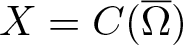 $X=C(\overline{\Omega})$ be an ordered Banach space, equipped with the maximum norm
 $\|\cdot\|$, and a positive cone
 \begin{equation*}X_+:=\{u\in X: u\geq0~\text{for all}~x\in\overline{\Omega})\}.\end{equation*}
Denote
 \begin{equation*}C_T:=\{u\in C(\overline{\Omega}\times\mathbb{R}): u(x,t)=u(x,t+T)~\text{for all}~(x,t)\in\overline{\Omega}\times\mathbb{R}\},\end{equation*}
and let
 \begin{equation*}C^+_T:=\{u\in C_T: u(x,t)\geq0~\text{for all}~(x,t)\in\overline{\Omega}\times\mathbb{R}\}.\end{equation*}
Below, let 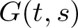 $G(t,s)$ be the evolution operator of the following system
 \begin{equation}
v_t+ \left(-d_v\Delta_N\right)^{s_2} v=-q(x,t) v, ~x\in \overline{\Omega}, ~t \gt 0.
\end{equation}
As in [Reference Peng and Zhao34], letting 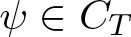 $\psi\in C_T$ be the density distribution of the infected individuals at time
 $\tau$ and the spatial location
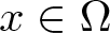 $x\in \Omega$, then
 $p(x,\tau)\psi(x,\tau)$ represents the density distribution of the new infections produced by the infected individuals at time
 $\tau$. Therefore,
 $G(t,\tau)p(x,\tau)\psi(x,\tau)$ is the density distribution at location
 $x$ of those infected individuals who were newly infected at time
 $\tau$ and remain infected at time
 $t$, where
 $t\geq \tau$. Consequently, the distribution of total new infections is
 \begin{equation*}
\int^t_{-\infty}G(t,\tau)p(\cdot,\tau)\psi(\cdot,\tau)d\tau=\int^\infty_{0}G(t,t-a)p(\cdot,t-a)\psi(\cdot,t-a)da.
\end{equation*}
Let  $L: C_T\mapsto C_T$ be the family bounded linear positive operators defined by
 \begin{equation}
L(\psi)(t):= \int^\infty_{0}G(t,t-a)p(\cdot,t-a)\psi(\cdot,t-a)da.
\end{equation}
We define the basic reproduction ratio for system (1.4) by the spectral radius of  $L$, that is,
 \begin{equation}
\mathcal{R}_0 := r(L).
\end{equation}
Now, consider the eigenvalue problem
 \begin{equation}
\begin{cases} \varphi_t+\left(-d_v\Delta_N\right)^{s_2} \varphi+q(x,t)\varphi=p(x,t)\varphi+\lambda\varphi, &x\in\overline{\Omega},~t \gt 0,\\
\varphi(x,T)=\varphi(x,0), & x \in \overline{\Omega}, \end{cases}
\end{equation}
and the linear weighted eigenvalue problem
 \begin{equation}
\begin{cases} \varphi_t+\left(-d_v\Delta_N\right)^{s_2} \varphi+q(x,t)\varphi= \frac{p(x,t)}{\mu}\varphi, &x\in\overline{\Omega},~t \gt 0,\\
\varphi(x,T)=\varphi(x,0), & x \in \overline{\Omega}, \end{cases}
\end{equation}
where  $\mu\in\mathbb{R}^+$. By [Reference Zhao and Ruan47, Theorem 3.3 and Proposition 4.9], we see that (2.4) has a unique principal eigenvalue
 $\lambda_0$ with a positive eigenfunction
 $\varphi_*\in C_T$, and (2.5) possesses a unique principal eigenvalue
 $\mu_d \gt 0$ with a positive eigenfunction
 $\varphi_0\in C_T$. Similar to [Reference Peng and Zhao34, Lemma 2.1] and [Reference Zhao and Ruan47, Proposition 4.9], we have the following results.
Proposition 2.1. The following statements hold.
(i)
 $\mathcal{R}_0=\mu_d$;
(ii)
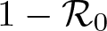
$1-\mathcal{R}_0$ has the same sign as
$\lambda_0$.


Proposition 2.2. The following conclusions hold.
(i) If
$p(x,t)\equiv p(t)$ and
$q(x,t)\equiv q(t)$, then
$\mathcal{R}_0=\int_0^Tp(t)dt/\int_0^Tq(t)dt$;(ii) If
$p(x,t)-q(x,t)\equiv a(t)$, then
$\mathcal{R}_0 \gt 1$ when
$\int_0^Ta(t)dt \gt 0$,
$\mathcal{R}_0=1$ when
$\int_0^Ta(t)dt=0$, and
$\mathcal{R}_0 \lt 1$ when
$\int_0^Ta(t)dt \lt 0$.


Proof. (i) We consider the following equation
 \begin{equation}
v_t=\left(-q(t)+\frac{1}{\mu_0}p(t)\right)v, ~~~~ v(0)=1,
\end{equation}
where  $\mu_0=\frac{\int_0^Tp(t)dt}{\int_0^Tq(t)dt}$. By a simple calculation, we can obtain that (2.6) has a unique positive solution
 $v(t)=e^{\int_0^t(-q(\tau)+\frac{1}{\mu_0}p(\tau))d\tau}$ satisfying
 $v(T)=v(0)=1$. Thus, (2.6) admits a positive
 $T$-periodic solution
 $v(t)$. Then, it follows from Proposition 2.1 and the uniqueness of principal eigenvalue
 $\mu_d$ of (2.5) that
 $\mathcal{R}_0=\mu_d=\mu_0$.
(ii) Now, consider the following problem
 \begin{equation}
v_t-a(t)v=\lambda v,~~~~ v(T)=v(0)=1.
\end{equation}
It is not difficult to check that (2.7) admits a unique positive solution if and only if  $\lambda=-\int_0^T a(t)dt$. Clearly,
 $v(t)=e^{\int_0^t(a(\tau)+\lambda)d\tau}$ is a positive
 $T$-periodic solution of (2.7). Note that
 $\lambda=-\int_0^T a(t)dt$ and
 $\varphi=e^{\int_0^t(a(\tau)+\lambda)d\tau}$ satisfy (2.4). Then, it follows from Proposition 2.1 and the uniqueness of principal eigenvalue
 $\lambda_0$ of (2.4) that (ii) holds true. This finishes the proof.
Next, we consider the case  $p(x,t)-q(x,t)=a(x)$ or
 $p(x,t)\equiv p(x)$ and
 $q(x,t)\equiv q(x)$. A similar proof can be found in [Reference Zhao and Ruan47, Propositions 2.2–2.3]. We first consider the situation of
 $p(x,t)-q(x,t)=a(x)$.
Proposition 2.3. Suppose that  $p(x,t)-q(x,t)=a(x)$. Then the following conclusions hold.
(i) If
$a(x)\not \equiv 0$ and
$\int_\Omega a(x)dx\geq0$, then
$\mathcal{R}_0 \gt 1$ for all
$d_v$;(ii) If
$a(x)\leq 0$ and
$\int_\Omega a(x)dx \lt 0$, then
$\mathcal{R}_0 \lt 1$ for all
$d_v$;(iii) If
$\max_{\overline{\Omega}}a(x) \gt 0$ and
$\int_\Omega a(x)dx \lt 0$, then there exists a threshold value
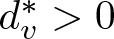
$d^*_v \gt 0$ such that
$\mathcal{R}_0 \gt 1$ when
$0 \lt d_v \lt d^*_v $ and
$\mathcal{R}_0 \lt 1$ when
$d_v \gt d^*_v $.




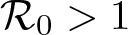


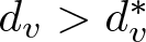
If  $p(x,t)\equiv p(x)$ and
 $q(x,t)\equiv q(x)$, similar to Allen et al. [Reference Allen, Bolker, Lou and Nevai1], we define the basic reproduction number
 $\mathcal{R}_0 $ for (1.4) by
 \begin{equation*}
\mathcal{R}_0=\sup \left\{\frac{ \int_{\Omega} p(x) \varphi^2 \mathrm{d} x}{\langle(-d_v\Delta_N)^{s_2} \varphi\mid \varphi\rangle+\int_\Omega q(x) \varphi^2 \mathrm{d} x}\Bigg|~ \varphi \in H^{s_2}(\Omega) \text {and } \varphi \neq 0\right\},
\end{equation*}
where  $\langle(-d_v\Delta_N)^{s_2} \varphi\mid \varphi\rangle=d_v^{s_2}\langle(-\Delta_N)^{s_2} \varphi\mid \varphi\rangle$, and
 $\langle(-\Delta_N)^{s_2} \varphi\mid \varphi\rangle$ is given in (1.5).
Proposition 2.4. Suppose that  $p(x,t)\equiv p(x)$ and
 $q(x,t)\equiv q(x)$. Then the following conclusions hold.
(i)
$ \int_{\Omega} p(x)dx/\int_\Omega q(x)dx\leq\mathcal{R}_0\leq \max\limits_{x\in\overline{\Omega}}[p(x)/q(x)]$;(ii) If
$\int_{\Omega} p(x)dx \lt \int_\Omega q(x)dx$ and
$p-q$ changes sign, then there exists a threshold value
$d^*_v \gt 0$ such that
$\mathcal{R}_0 \gt 1$ when
$0 \lt d_v \lt d^*_v $ and
$\mathcal{R}_0 \lt 1$ when
$d_v \gt d^*_v $;(iii)
$\mathcal{R}_0\rightarrow \max\limits_{x\in\overline{\Omega}}[p(x)/q(x)]$ as
$d_v\rightarrow0^+$ and
$\mathcal{R}_0\rightarrow \int_{\Omega} p(x)dx/\int_\Omega q(x)dx$ as
$d_v\rightarrow\infty$;(iv) Let
$\lambda_2$ be the second least eigenvalue of
$-\Delta_N$ in
$\Omega$. If
$d_v\lambda_2\geq1$, then
$\mathcal{R}_0$ is non-increasing in
$s_2$; if
$d_v\lambda_2 \gt 1$, then
$\mathcal{R}_0$ is monotone decreasing function of
$s_2$.


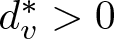
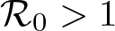


Now, we study some properties of  $\mathcal{R}_0$ under the general case of
 $p(x,t)$ and
 $q(x,t)$.
Proposition 2.5. The following conclusions hold.
(i)
$ \int_0^T\int_{\Omega} p(x,t)dxdt/\int_0^T\int_\Omega q(x,t)dxdt\leq\mathcal{R}_0$, and the strict inequality holds if and only if
$p(x,t)-q(x,t)$ nontrivially depends on
$x$. In addition,
$\mathcal{R}_0\leq \frac{\max_{\overline{\Omega}\times[0,T]}p(x,t)}{\min_{\overline{\Omega}\times[0,T]}q(x,t)} $;(ii) If
$p(x,t)-q(x,t)$ nontrivially depends on
$x$ and
$\int_0^T\max_{x\in\overline{\Omega}}[ p(x,t)-q(x,t)]dt\leq0$, then
$\mathcal{R}_0 \lt 1$ for all
$d_v$;(iii)
$\mathcal{R}_0\rightarrow \max\limits_{x\in\overline{\Omega}} \frac{\int_0^T p(x,t)dt}{\int_0^Tq(x,t)dt} $ as
$d_v\rightarrow0^+$;(iv)
$\mathcal{R}_0\rightarrow \int_0^T\int_{\Omega} p(x,t)\psi_1(x)\psi_2(x)dxdt/\int_0^T\int_\Omega q(x,t)\psi_1(x)\psi_2(x)dxdt~\text{as}~d_v\rightarrow\infty,$ where
$\psi_1\in \operatorname{ker}\left(\Delta_N\right)$,
$\psi_2 \in \operatorname{ker}\left(\mathcal{L}\right)$ with
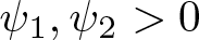
$\psi_1, \psi_2 \gt 0$ and
$\left\langle\psi_1, \psi_2\right\rangle=1$, here
$\mathcal{L }$ is the formal adjoint operator of
$\Delta_N$.(v) In general,
$\mathcal{R}_0\left(d_v\right):=\mathcal{R}_0$ is not a non-increasing function with respect to
$d_v$; in particular, if
$p(x, t)= p_0(x)p_1(t)$ and
$q(x, t)=p_0(x)p _2(t)$ with
$p_0 \gt 0$ on
$\bar{\Omega}, p_0 \not \equiv$ constant ,
$p_1, p_2 \in C_T$ and
$ p_1, p_2 \gt 0$ on
$[0, T]$ with
$p_1-p_2 \not \equiv$ constant, then there exist
$0 \lt d_v^1 \lt d_v^2$ such that
$\mathcal{R}_0\left(d_v^1\right)=\mathcal{R}_0\left(d_v^2\right)$.












(i) Let
$\varphi_0$ be a positive eigenfunction corresponding to
$\mu_d$. Multiplying the first equation of (2.5) by
$\varphi_0^{-1}$, and integrating the resulting equation over
$ \Omega \times(0,T)$, we have
(2.8)\begin{align}
0\geq\int_0^T \langle(-d_v\Delta_N)^{s_2} \varphi_0\mid \varphi_0^{-1}\rangle dt =-\int_0^T\int_\Omega q(x,t)dxdt + \int_0^T\int_\Omega \frac{p(x,t)}{\mathcal{R}_0}dxdt.
\end{align}Here we used the fact that
$\langle(-d_v\Delta_N)^{s_2} \varphi_0\mid \varphi_0^{-1}\rangle\leq0$ (see Section 2 in [Reference Zhao and Ruan46]) and
$\mathcal{R}_0=\mu_d$. This completes (i).(ii) Let
$p(x,t)-q(x,t)=m(x,t)$. Then, similar to the arguments of [Reference Peng and Zhao34, Theorem 2.5], we have
this together with Proposition 2.1 immediately yield (ii).
\begin{equation*}
\lambda_0 \gt -\frac{1}{T }\int_0^T\max_{x\in\overline{\Omega}} [p(x,t)-q(x,t)] dt\geq0,
\end{equation*}


Assertions (iii) and (iv) follow from [Reference Zhao and Ruan47, Proposition 4.9]. The desired conclusion (v) follows from (iii) and (iv). This finishes the proof.
Next, we establish the global existence of solutions and point dissipativity of (1.4). We say that  $u \gneq v$ means that
 $u \geq v$ and
 $u$ and
 $v$ are not identical. Similar to Zhao and Ruan [Reference Zhao and Ruan46, Proposition 3.2] (see also Shi et al. [Reference Shi, Li and Yang37, Theorem 4.1]), we have the following result.
Theorem 2.6 Suppose that  $\left(u_0, v_0 \right) \in X_+\times X_+$. Then
 $(1.4)$ admits a unique global solution
 $\left(u (t,u_0,v_0), v(t,u_0,v_0)\right)$ such that
 $u (0,u_0,v_0)(x)=u_0(x)$ and
 $v (0,u_0,v_0)(x)=v_0(x)$. Moreover,
 $u (t,u_0,v_0) \gt 0$ and
 $v(t,u_0,v_0) \gt 0$ on
 $\overline{\Omega}$ for each
 $t \gt 0$ if
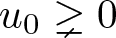 $u_0 \gneq 0$ and
 $ v_0 \gneq 0$. In particular,
 \begin{equation}
\limsup _{t \rightarrow \infty}\left|u (t,u_0,v_0) \right|_{\infty} \leq C, \quad \limsup _{t \rightarrow \infty}\left|v(t,u_0,v_0) \right|_{\infty} \leq C,
\end{equation}
where  $C \gt 0$ is a constant depending on
 $d_u, d_{v }, s_i(i=1,2), n$ and
 $p , q $.
We say  $\left(\tilde{u},\tilde{v}\right)$ is an
 $T$-periodic solution of
 $(1.4)$ if it is a nonnegative classical solution of
 \begin{equation}
\begin{cases}u_t+\left(- d_u\Delta_N\right)^{s_1} u= -\frac{p(x,t) u v}{u+v}+q(x,t) v, & x\in \overline{\Omega}, ~t\in\mathbb{R}, \\
v_t+ \left(-d_v\Delta_N\right)^{s_2} v=\frac{p(x,t)u v}{u+v}-q(x,t) v, & x\in \overline{\Omega}, ~t\in\mathbb{R}, \\
u( x, t)=u (x, t+T), v( x, t)=v(x, t+T), & x \in \overline{\Omega}, ~t\in\mathbb{R},\\
\int_\Omega(u_0+v_0)dx=N. \end{cases}
\end{equation}
Recalling, we say that the solution  $\left(\tilde{u},\tilde{v}\right)$ of (2.10) is the disease-free
 $T$-periodic solution of
 $(1.4)$ if
 $\tilde{u} \gt 0$ and
 $\tilde{v}\equiv0$, and the solution
 $\left(\tilde{u},\tilde{v}\right)$ of (2.10) is the endemic
 $T$-periodic solution of (2.10) if
 $\tilde{u} \gt 0$ and
 $\tilde{v}\gneq0$. By Theorem 2.6, we have
 $ \tilde{u},\tilde{v} \in\operatorname{Int} C_T^{+}$ if
 $\left(\tilde{u},\tilde{v}\right)$ is an endemic periodic solution of
 $(1.4)$. We next show that there is a DFE of system
 $(1.4)$.
Proposition 2.7. System  $(1.4)$ has a unique DFE
 $( \hat{u} ,0)$, where
 $\hat{u}=\frac{N}{|\Omega|}$.
Proof. Letting  $( \hat{u} ,0)$ be any DFE, we have
 \begin{equation*}
\begin{cases}\hat{u}_t+\left(- d_u\Delta_N\right)^{s_1} \hat{u}= 0, & x\in \overline{\Omega}, t\in\mathbb{R}, \\
\hat{u}( x, t)=\hat{u}(x, t+T), \int_\Omega\hat{u}(x,t)dx=N, & x \in \overline{\Omega}, t\in\mathbb{R}.
\end{cases}
\end{equation*}
As in the proof of [Reference Shi, Li and Yang37, Theorem 4.6], we have  $\hat{u}(x,t)\rightarrow \frac{1}{|\Omega|}\int_\Omega\hat{u}_0(x)dx$ uniformly on
 $\overline{\Omega}$ as
 $t\rightarrow\infty$. Thus,
 \begin{equation*}\hat{u}(x,t)-\frac{N}{|\Omega|}=\lim_{n\rightarrow+\infty}\hat{u}(x,t+nT)-\frac{N}{|\Omega|}=0 ~\text{for all}~x\in \overline{\Omega}~\text{and}~ t\in[0,T].\end{equation*}
The proof is finished.
Definition 2.8. A solution  $\left(\tilde{u},\tilde{v}\right)$ of
 $(2.10)$ is said to be globally asymptotically stable if
 \begin{equation*}\lim_{t\rightarrow+\infty}\|(u (t,u_0,v_0), v(t,u_0,v_0))-\left(\tilde{u},\tilde{v}\right)\|_{C(\overline{\Omega})\times C(\overline{\Omega})}=0,\end{equation*}
where  $(u (t,u_0,v_0), v(t,u_0,v_0))$ is the solution of
 $(1.4)$ and
 $(u_0,v_0)\in X_+\times X_+$.
Then, we have the following dynamic behaviour of system  $(1.4)$.
Theorem 2.9 The following statements hold.
(i) If
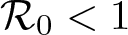
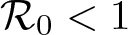
$ \mathcal{R}_0 \lt 1$, then
$(\frac{N}{|\Omega|}, 0)$ is globally asymptotically stable;(ii) If
$ \mathcal{R}_0 \gt 1$, then there exists a positive constant
$\eta$ such that
(2.11)where\begin{equation}
\liminf _{t \rightarrow \infty} u (t,u_0,v_0) \geq\eta ~\text{and}~ \liminf_{t \rightarrow \infty} v(t,u_0,v_0) \geq\eta,
\end{equation}
$(u (t,u_0,v_0), v(t,u_0,v_0))$ is the solution of
$(1.4)$. Moreover,
$(1.4)$ admits at least one endemic
$T$-periodic solution.


(i) By the second equation of
$(1.4)$ and the facts that
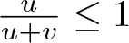
$\frac{u}{u+v}\leq1$, we have
\begin{equation*}\partial_tv+\left(- d_{v}\Delta_N\right)^{s_2} v \leq[p -q ] v.\end{equation*}Following a similar approach as in Proposition 2.5, set
$\varphi_1$ to be the positive eigenfunction corresponding to
$\lambda_0$. Take
$\phi=C_{v}e^{-\lambda_0t}\varphi_1$, where
$C_{v}=\max\{C, |v_0|_{\infty}\}$ and
$C$ is obtained in Theorem 2.6. Thus
\begin{equation*}\partial_t\phi+\left(- d_{v}\Delta_N\right)^{s_2} \phi=[p -q] \phi.\end{equation*}By the comparison principle (see [Reference Zhao and Ruan47, Proposition 5.1]), we have
\begin{equation*} v(t,u_0,v_0)\leq C_{v}e^{-\lambda_0t}\varphi_1, ~x\in\overline{\Omega}.\end{equation*}Since
$\mathcal{R}_{0} \lt 1$, we can see that
$\lambda_0 \gt 0$. Thus, we have
$\lim_{t\rightarrow\infty}\|v(t,u_0,v_0)\|_{C(\overline{\Omega})}=0$.Next, we show that
$u(t,u_0,v_0)$ converges to
$\frac{N}{|\Omega|}$ as
$t\rightarrow\infty$. By the first equation of
$(1.4)$, we have
\begin{equation*}\partial_tu+\left(- d_u\Delta_N\right)^{s_1} u=\left[q -\frac{pu}{u+v}\right]v,~(t, x) \in \mathbb{R}^{+} \times \overline{\Omega}.\end{equation*}Since
$ v(t,x)\leq C_{v}e^{-\lambda_0t}\varphi_1, ~x\in\overline{\Omega} $, there is
where
\begin{equation*}\left|\partial_tu+\left(- d_u\Delta_N\right)^{s_1} u\right|\leq C_{0}e^{-\lambda_0t}, ~(t, x) \in \mathbb{R}^{+} \times \overline{\Omega},\end{equation*}
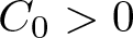
$C_{0} \gt 0$ is some constant. Then
$u(t,x)$ tends towards a positive constant as
$t\rightarrow\infty$. Indeed, let
$u(x,t)=\tilde{u}(t)+\hat{u}(t,x)$, where
$\tilde{u}(t):=\frac{1}{|\Omega|}\int_\Omega u(t,x)dx$. By a simple calculation, we can obtain
\begin{equation*} \partial_t\tilde{u}=\frac{1}{|\Omega|}\int_\Omega \partial_tu(t,x)dx=\frac{1}{|\Omega|}\int_\Omega \left[q -\frac{pu}{u+v}\right]vdx, ~(t, x) \in \mathbb{R}^{+} \times \overline{\Omega}.\end{equation*}Observe that
$|\partial_t\tilde{u}|\leq C_*e^{-\lambda_0t}$, where
$C_*$ is a positive constant. Thus, we can see that
$\hat{u}$ satisfies
(2.12)where\begin{equation}
\begin{cases}\partial_t\hat{u}+d_u\left(- \Delta_N\right)^{s} \hat{u}=g(t,x), & (t, x) \in \mathbb{R}^{+} \times \overline{\Omega}, \\ \int_\Omega\hat{u}(t,x)dx\equiv0, & t\geq0,\end{cases}
\end{equation}
$|g(t,x)|\leq C^*e^{-\lambda_0t}$ for some positive constant
$C^*$. Subsequently, it follows from
$N=\int_\Omega(u + v )dx$ and
$\lim_{t\rightarrow\infty}\|v(t,u_0,v_0)\|_{C(\overline{\Omega})}=0$ that
$\lim_{t\rightarrow\infty}\|\tilde{u} (t)\|_{C(\overline{\Omega})}=\frac{N}{|\Omega|}$. Now, we prove
$\hat{u}(t,x)\rightarrow0$ for
$x\in\Omega$ as
$t\rightarrow\infty$. Set
$0=\lambda_0^* \lt \lambda_1 \lt \lambda_2\leq\ldots$ represent the eigenvalues of
$\left(- \Delta_N\right)^{s}$ and
$\{\varphi_m\}_{m=0}^{+\infty}$ denote the corresponding (normalized) eigenfunctions (see, e.g., [Reference Pellacci and Verzini30, Proposition A.1]). Letting
$\hat{u}=\Sigma^{+\infty}_{m=0}a_m(t)\varphi_m(x)$ and
$g=\Sigma^{+\infty}_{m=0}g_m(t)\varphi_m(x)$, and noting that
$\int_\Omega\hat{u}(t,x)dx\equiv0$, we can obtain that
$a_0=0$. Furthermore, integrating
$(2.12)$ on
$\Omega$, we can also obtain
$g_0=0$. Since
$|g(t,x)|\leq C^*e^{-\lambda_0t}$, it is not difficult to see that there exists
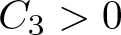
$C_3 \gt 0$ such that
$|g_m(t)|\leq C_3e^{-\lambda(d_{v},p-q)t}$ for all
$m\geq1$. For any
$m\geq1$, we rewrite
$(2.12)$ as
$\frac{d}{dt}(\Sigma^{+\infty}_{m=0}a_m(t)\varphi_m(x))+d_u ( \Sigma^{+\infty}_{m=1}\lambda_ma_m(t)\varphi_m(x))=\Sigma^{+\infty}_{m=1}g_m(t)\varphi_m(x)$ for
$t \gt 0$ and
$x \in \overline{\Omega}$. It can be easily seen that there exists
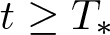
$T_*$ such that
$\frac{d}{dt}\hat{u}\leq-d_u\lambda_* \hat{u} $ for
$t\geq T_*$ and
$x \in \overline{\Omega}$, where
$\lambda_*=\min\{\lambda_1,\lambda_0\}$. Then, it can be shown that
$\hat{u}(t,x)\rightarrow0$ as
$t\rightarrow\infty$ for all
$x\in\Omega$, and this together with
$\lim_{t\rightarrow\infty}\|\tilde{u} (t)\|_{C(\overline{\Omega})}=\frac{N}{|\Omega|}$ yields that
$\lim_{t\rightarrow\infty} \left\|u(t,\cdot)-\frac{N}{|\Omega|}\right\|_{C(\overline{\Omega})}=0$.(ii) We will validate the validity of our conclusions using abstract dynamical system theory (see, e.g., [Reference Zhao48]). As in [Reference Peng and Zhao34] and [Reference Zhao and Ruan47], let
$\mathcal{A}=L^p(\Omega)(1 \lt p \lt \infty)$,
$\mathcal{A}^\theta=\mathcal{D}(\left(-\Delta_N\right)^\theta )(\frac{1}{2}+\frac{1}{2p} \lt \theta \lt 1)$ and
$\mathcal{A}^+$ is a cone composed of all nonnegative functions in
$\mathcal{A}^\theta$, where
$\mathcal{D}(\left(-\Delta_N\right)^\theta )$ is the domain of
$\left(-\Delta_N\right)^\theta$. Then Int
$\mathcal{A}^+$ is non-empty and
$\mathcal{A}^\theta $ compactly embeds into
$\left\{w \in C^{1,\alpha}(\Omega): \frac{\partial w}{\partial \nu} \Big|_{\partial \Omega}=0\right\}$ if
$1/2+1/2p \lt \theta \lt 1$ and
$0\leq\alpha \lt 2\theta-1-\frac{1}{p}$. Denote
\begin{equation*}X_0:=\left\{(u , v ) \in \mathcal{A}\times \mathcal{A}: \int_\Omega (u +v )dx\equiv N~\text{and}~ u , v \in \text{Int}\mathcal{A}^+\right\}.\end{equation*}By Theorem 2.6, for any
$(u_0,v_0)\in X_0$, we have
$(1.4)$ that admits a unique global solution
$U(t,(u_0,v_0))=(u (t,u_0,v_0), v(t,u_0,v_0))$. Let
$\Psi: X_0 \rightarrow X_0$ be an
$T$-semiflow induced by the solution of
$(1.4)$, i.e.
$\Psi(t)(u_0,v_0):=U(t,(u_0,v_0))$ for any
$t\geq0$, and let
$X_1:=\left\{(u_0 , v_0) \in X_0: v_0 \not \equiv0 \right\}$ and
$\partial X_1:=\left\{(u_0 , v_0) \in X_0: v_0\equiv0 \right\}$, then
$X_0= X_1\cup \partial X_1$,
$ \Psi(t) X_1\subset X_1$ and
$ \Psi(t) \partial X_1\subset\partial X_1$ for all
$t\geq0$. By Theorem 2.6, we have
$ \Psi(t)$ is point dissipative. Similar to the proof of [Reference Zhao and Ruan47, Theorem 3.3] (or see page 264 of [Reference Zhao and Ruan46]), we have
$\Psi: X_0 \rightarrow X_0$ be continuous and compact for all
$t \gt 0$.



















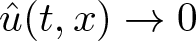
















We define the Poincaré map  $\Phi: X_0 \rightarrow X_0$ by
 $\Phi (u_0,v_0) :=\Psi(T)( u_0,v_0)$ for any
 $(u_0,v_0)\in X_0$, then
 $\Phi: X_0 \rightarrow X_0$ is point dissipative, continuous and compact. Subsequently, it follows from [Reference Zhao48, Theorem 1.1.3] that
 $\Phi$ has a global attractor. For convenience, we let
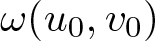 $\omega(u_0,v_0)$ be the limit set related to
 $ (u_0,v_0)\in X_0$. If
 $(u_0,v_0)\in \partial X_0$, we can see that
 \begin{equation*}
\begin{cases} u_t+\left(- d_u\Delta_N\right)^{s_1} u= 0, & x\in \overline{\Omega},~ t \gt 0, \\
u ( x, 0)= u_0(x) \gneq 0, \int_\Omega u (x,t)dx=N, & x \in \overline{\Omega},~ t \gt 0.
\end{cases}
\end{equation*}
As in the proof of Proposition 2.7, we obtain that  $u(x,t)\rightarrow \frac{N}{|\Omega|}$ uniformly on
 $\overline{\Omega}$ as
 $t\rightarrow\infty$. This implies
 $\bigcup_{(u_0,v_0)\in \partial X_0}\omega(u_0,v_0)=\{E_0\}$, where
 $E_0=(\frac{N}{|\Omega|},0)$. Next, we claim that there exists a real number
 $\eta_0 \gt 0$ such that
 \begin{equation} \limsup_{m\rightarrow+\infty}\|\Phi^m (u_0,v_0)-E_0\|_{\mathcal{A}\times \mathcal{A}}\geq\eta_0~\text{for all}~(u_0,v_0)\in X_0, \end{equation}
where  $\Phi^m (u_0,v_0)=U(mT, (u_0,v_0))$. On the contrary, we suppose that (2.13) is false. Then, there exists
 $m_0 \gt 0$ such that
 \begin{equation*}\frac{N}{|\Omega|}-\eta_0 \lt u (t,u_0,v_0) \lt \frac{N}{|\Omega|}+\eta_0,~ 0 \lt v (t,u_0,v_0) \lt \eta_0,~ t\geq m_0.\end{equation*}
Since  $ \mathcal{R}_0 \gt 1$, by Proposition 2.1, we have
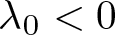 $\lambda_0 \lt 0$. Denote
 $\lambda_0(\varepsilon)$ be the principal eigenvalue of
 \begin{equation*}
\begin{cases} \varphi_t+\left(-d_v\Delta_N\right)^{s_2} \varphi+q(x,t)\varphi=\frac{p(x,t)(N/|\Omega|-\varepsilon)}{N/|\Omega|+2\varepsilon }\varphi+\lambda\varphi, &x\in\overline{\Omega},~t \gt 0,\\
\varphi(x,0)=\varphi(x,T), & x \in \overline{\Omega}. \end{cases}
\end{equation*}
If  $\varepsilon$ is small enough, we find
 $\lambda_0(\varepsilon) \lt 0$. Let
 $\phi_0$ be a positive eigenfunction corresponding to
 $\lambda_0(\varepsilon)$. Then, there exists
 $c_* \gt 0$ sufficiently small such that
 $c_*\phi_0\leq v (m_0,u_0,v_0)$. For
 $t\geq m_0$ and
 $\eta_0 \lt \varepsilon$,
 $v(t,u_0,v_0)$ is a supersolution of
 \begin{equation}
\begin{cases} \tilde{\varphi}_t+\left(-d_v\Delta_N\right)^{s_2} \tilde{\varphi}+q(x,t) \tilde{\varphi}=\frac{p(x,t)(N/|\Omega|-\varepsilon)}{N/|\Omega|+2\varepsilon } \tilde{\varphi}, &x\in\overline{\Omega},~t \gt m_0,\\
\tilde{\varphi}(x,m_0)=c_*\phi_0, & x \in \overline{\Omega}. \end{cases}
\end{equation}
It can be seen that  $c_*e^{-\lambda_0(\varepsilon)(t-m_0)}\phi_0$ is the unique solution of (2.14). Subsequently, it follows from the comparison principle that
 $v(t,u_0,v_0)\geq c_*e^{-\lambda_0(\varepsilon)(t-m_0)}\phi_0\rightarrow\infty$ uniformly for
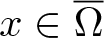 $x\in\overline{\Omega}$ as
 $t\rightarrow\infty$. This shows that
 $v(t,u_0,v_0)$ is unbounded, a contradiction to Theorem 2.6 and this proves the claim. And the remaining proof is the same as that in [Reference Peng and Zhao34, Theorem 3.3].
The following theorem provides criteria for the existence and extinction of diseases. This can be directly inferred from Propositions 2.3–2.5 and Theorem 2.9.
Theorem 2.10 The following statements hold for (1.4).
(i) If one of the following conditions holds:
(i.-1)
$p(x,t)-q(x,t)\equiv a(t)$ and
$\int_0^Ta(t)dt \lt 0$;(ii.-1)
$p(x,t)-q(x,t)\equiv a(x) \lneq 0$ on
$\overline{\Omega}$ or
$\max_{\overline{\Omega}}a(x) \gt 0$,
$\int_\Omega a(x)dx \lt 0$ and
$d_v \gt d^*_v $;(iii.-1)
$p(x,t)-q(x,t)$ nontrivially depends on
$x$ and
$\int_0^T\max_{x\in\overline{\Omega}}[ p(x,t)-q(x,t)]dt\leq0$;(iv.-1)
$\int_0^T\int_{\Omega} p(x,t)-q(x,t)dxdt \lt 0$ and
$d_v\geq d^*$, where
$d^*$ is a positive constant and large enough;








Then 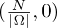 $(\frac{N}{|\Omega|}, 0)$ is globally asymptotically stable.
(ii) If one of the following statements holds:
(i.-1)
$p(x,t)-q(x,t)\equiv a(t)$ and
$\int_0^Ta(t)dt \gt 0$;(ii.-1)
$p(x,t)-q(x,t)\equiv a(x)$, either
$a(x)\gneq 0$ or
$\max_{\overline{\Omega}}a(x) \gt 0$,
$\int_\Omega a(x)dx \lt 0$ but
$0 \lt d_v \lt d^*_v $;(iii.-1)
$\int_0^T\int_\Omega[ p(x,t)-q(x,t)]dxdt \gt 0$;(iv.-1)
$ \max_{x\in\overline{\Omega}} \int_0^T[p(x,t) - q(x,t)] dt \gt 0$ and
$d_v\leq d_*$, where
$d_*$ is a positive constant and small enough.





Then  $(2.11)$ holds.
Now, we recall the results that can be found in [Reference Peng and Zhao34].
Lemma 2.11. Assume that  $a_0$ and
 $a_1$ are two positive constants, and
 $\phi_0, \phi_1 \in C^1([a_0, \infty)), \phi_1\geqslant 0$ and
 $\phi_0$ is bounded from below on
 $[a_0, \infty)$. If
 $\phi_0^{\prime}(t) \leqslant-a_1 \phi_1(t)$ and
 $\phi_1'(t) \leqslant M$ in
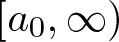 $[a_0, \infty)$ for some constant
 $M \gt 0$, then
 $\lim _{t \rightarrow \infty} \phi_1=0$.
Our next result is the impact of the local distribution of transmission and recovery rates on disease dynamics.
Theorem 2.12 Assume that  $p(x,t)=rq(x,t)$ on
 $\overline{\Omega}\times\mathbb{R}$ for some positive constant
 $r$. If
 $r\leq1$, then
 $(\frac{N}{|\Omega|}, 0)$ is globally asymptotically stable; if
 $r \gt 1$, then
 $(\tilde{u}, \tilde{v})=\left(\frac{N}{r|\Omega|}, \frac{(r-1)N}{r|\Omega|}\right)$ is globally attractive.
Proof. By Proposition 2.1 and (2.5), we have  $\mathcal{R}_0=r$. Thus, Theorem 2.9 shows that
 $(\frac{N}{|\Omega|}, 0)$ is globally asymptotically stable when
 $r \lt 1$. Next, we discuss the case
 $r = 1$, that is
 $p(x,t)= q(x,t)$. By (1.4), we have
 \begin{equation}
\begin{cases}u_t+\left(- d_u\Delta_N\right)^{s_1} u= \frac{p(x,t) v^2}{u+v}, & x\in \overline{\Omega}, t \gt 0, \\
v_t+ \left(-d_v\Delta_N\right)^{s_2} v=-\frac{p(x,t)v^2}{u+v}, & x\in \overline{\Omega}, t \gt 0, \\
u(0, x)=u_0(x), v(0, x)=v_0(x), & x \in \overline{\Omega}, \end{cases}
\end{equation}
where  $(u,v)$ is the solution of (1.4). We claim that
 $\|u(\cdot,t)\|_X\leq \tilde{C}_1$ and
 $\|v(\cdot,t)\|_X\leq \tilde{C}_1$ for all
 $t\geq0$ and some positive constant
 $\tilde{C}_1$. Noticed that the following equation
 \begin{equation}
\left\{\begin{array}{l}
w_t+\left(- d_v\Delta_N\right)^{s_2} w=0, ~ x \in \overline{\Omega}, \ t \gt 0, \\ w(0, x)=v_0(x), ~x\in\overline{\Omega}
\end{array}\right.
\end{equation}
admits a unique solution  $w(x,t)$ for all
 $x\in \bar{\Omega}$ and
 $t \gt 0$. And obviously,
 $v$ and
 $\max_{x\in\overline{\Omega}}v_0(x)$ are the bounded super-solution and sub-solution of system (2.16), respectively. It then follows from the comparison principle that
 \begin{equation} v(x,t)\leq w(x,t)\leq \max_{x\in\overline{\Omega}}v_0(x)~\text{for all }~x\in\overline{\Omega}~\text{and}~t\geq0.\end{equation}
We next turn to  $u$. By the first equation of (2.15), we find that
 \begin{equation*}u(x, t)=e^{- \left(-d_u\Delta_N\right)^{s_1} t} u(x,0)+\int_0^t e^{-\left(- d_u\Delta_N\right)^{s_1}(t- \tau)} f(u,v) d \tau,\end{equation*}
where  $f(u,v)=\frac{p(x,t) v^2}{u+v}$. Subsequently, it follows from [Reference Zhao and Ruan46, Lemma 3.1] and (2.17) that
 $\|u(\cdot,t)\|_X\leq \tilde{C}_1$ for all
 $t\geq0$. Let
 $p_1$ and
 $p_2$ be two positive constants and
 $p_1\leq p \leq p_2$. We consider the following problem
 \begin{equation}
\left\{\begin{array}{l}
\bar{u}_t=\frac{p_2 \bar{v}^2}{\bar{u}+\bar{v}}, ~ x \in \overline{\Omega}, \ t \gt 0, \\
\bar{v}_t=-\frac{p_1 \bar{v}^2}{\bar{u}+\bar{v}}, ~ x \in \overline{\Omega}, \ t \gt 0, \\ \bar{u}(0)=\max\limits_{x\in \overline{\Omega}}u_0(x), \bar{v}(0)=\min\limits_{x\in \overline{\Omega}}v_0(x), ~x\in\overline{\Omega}.
\end{array}\right.
\end{equation}
It is easily seen that (2.18) has a unique positive solution  $(\bar{u},\bar{v})$,
 $\bar{u}$ is increasing and
 $\bar{v}$ is decreasing in
 $t$. Simple calculation shows that
 $\bar{u}_t=-p_2p_1^{-1}\bar{v}_t$, which implies that
 \begin{equation*}\bar{u}(t)-\bar{u}(0)=-p_2p_1^{-1}[\bar{v}(t)-\bar{v}(0)]~\text{for all}~t\geq0.\end{equation*}
Observe that  $\bar{v}(t)\leq\bar{v}(0)$ for all
 $t\geq0$. Thus, there exists a positive constant
 $\tilde{C}_2$ such that
 \begin{equation*}\bar{u}(t)+\bar{v}(t)\leq \tilde{C}_2~\text{for all}~t\geq0.\end{equation*}
Next, we prove  $\bar{v}(t)\rightarrow0$ as
 $t \rightarrow\infty$. Indeed, there are
 $\bar{u}^*$ and
 $ \bar{v}^*$ such that
 $\bar{u}(t)\rightarrow \bar{u}^*$ and
 $\bar{v}(t)\rightarrow \bar{v}^*$ as
 $t \rightarrow\infty$. If
 $\bar{v}^* \gt 0$, we have
 \begin{equation*}\bar{u}_t=\frac{p_2 \bar{v}^2}{\bar{u}+\bar{v}}\rightarrow\frac{p_2 (\bar{v}^*)^2}{\bar{u}^*+\bar{v}^*}~\text{as}~t\rightarrow\infty.\end{equation*}
This implies 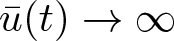 $\bar{u}(t)\rightarrow\infty$ as
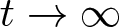 $t\to\infty$, a contradiction. Hence, we can obtain that
 $\bar{v}(t)\rightarrow0$ as
 $t \rightarrow\infty$. On the other hand, we notice that
 $(\bar{u},\bar{v})$ is the super-solution of (2.15). Therefore, we obtain
 \begin{equation*}u(x,t)\leq\bar{u}(t)~\text{and}~ v(x,t)\leq\bar{v}(t)~\text{for all}~t\geq0.\end{equation*}
That is,  $\lim\limits_{t\rightarrow\infty}\|v(\cdot,t)\|_{X}=0$. It then follows from (H2) that
 $\int_\Omega u(x,t)dx\rightarrow N$ as
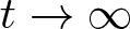 $t\rightarrow\infty$. Now, we prove
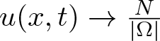 $u(x,t)\rightarrow \frac{N}{|\Omega|}$ uniformly for
 $x\in\overline{\Omega}$ as
 $t \rightarrow\infty$. Let
 \begin{equation*} \check{u}(t):=\frac{1}{|\Omega|}\int_\Omega u(t,x)dx ~\text{and}~ \hat{u}(x,t)= u(x,t)-\check{u}(t).\end{equation*}
By a simple calculation, we have
 \begin{equation}
\hat{u}_t+\left(- d_u\Delta_N\right)^{s_1}\hat{u}=\frac{p(x,t) v^2}{u+v}-\frac{1}{|\Omega|}\int_\Omega\frac{p(x,t) v^2}{u+v}dx~\text{for all }~x\in\overline{\Omega}~\text{and}~t \gt 0.
\end{equation}
We take  $g(x,t)=\frac{p(x,t) v^2}{u+v}-\frac{1}{|\Omega|}\int_\Omega\frac{p(x,t) v^2}{u+v}dx$. It then follows from
 $\lim\limits_{t\rightarrow\infty}\|v(\cdot,t)\|_{X}=0$ that
 $\lim\limits_{t\rightarrow\infty}\|g(\cdot,t)\|_{X}=0$. Letting
 $f(t)=\int_\Omega \hat{u}(x,t) g(x,t)dx$, we can easily verify that
 $|f(t)|\rightarrow0$ as
 $t\rightarrow\infty$ since
 $|\hat{u}|\leq2\tilde{C}_1$. Setting
 $\kappa(t)=\int_\Omega\hat{u}^2(x,t)dx$ and noting that
 $K_{s}(x, y)$ enjoys two-sided Gaussian estimates, one can see that there exists a positive constant
 $C^*_1$(depending on
 $n$,
 $|\Omega|$ and
 $\tilde{C}_1$ ) and there is a
 $t_0 \gt 0$ such that
 \begin{align*}
\frac{\partial\kappa}{\partial t}&=2\int_\Omega\hat{u}(x,t)\frac{\partial\hat{u}(x,t)}{\partial t}dx
=- 2d_u^{s_1}\int_{\Omega} \int_{\Omega} K_{s}(x, y)[\hat{u}(x,t)-\hat{u}(y,t)]^2 d y d x+2f(t)\\
&\leq - 2d_u^{s_1}C^*_1\kappa(t)+2f(t), ~t\geq t_0.
\end{align*}
Thus,
 \begin{equation*}\kappa(t)\leq e^{- 2d_u^{s_1}C^*_1t}\kappa(t_0)+2e^{- d_u^{s_1}C^*_1t}\int_{t_0}^te^{- 2d_u^{s_1}C^*_1\tau}f(\tau)d\tau.\end{equation*}
This implies  $\kappa(t)\rightarrow0$ as
 $t\rightarrow\infty$. That is,
 $\lim\limits_{t\rightarrow\infty}\|u -\check{u} \|_{L^2(\Omega)}=0$. Next, we show that
 \begin{equation*} |u -\check{u} |_{\infty}\leq C\|u -\check{u} \|_{L^2(\Omega)}, \end{equation*}
where  $C \gt 0$ is a constant. Without loss of generality, we let
 $d_u=1$ and
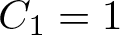 $C_1=1$(
 $C_1$is given by (1.6)). For
 $m\geq2$, multiplying the equation of (2.19) by
 $\hat{u}^{m-1}$ and integrating over
 $\Omega$, we find that
 \begin{align*}
&\frac{1}{m}\frac{d}{dt}\int_\Omega \hat{u}^{m}dx+\frac{4(m-1)}{m^2}\left\|\hat{u}^{\frac{m}{2}}\right\|^2_{H^{s_1}
(\Omega)}\\
\leq& \int_\Omega g(x,t)|\hat{u}|^{m-1}dx\\
\leq& \left(\int_\Omega |g(x,t)|^mdx\right)^{\frac{1}{m}}\left(\int_\Omega |\hat{u}|^{m }dx\right)^{\frac{m-1}{m}}\\
\leq& \tilde{C}^*_1\left(\int_\Omega |\hat{u}|^{m }dx\right)^{\frac{m-1}{m}},
\end{align*}
where  $\tilde{C}^*_1 \gt 0$ depends on
 $\tilde{C}_1$,
 $|p(x,t)|_\infty$ and
 $|\Omega|$. Letting
 $\tilde{w}=\hat{u}^{\frac{m}{2}}$, then
 \begin{equation} \frac{d}{dt}\int_\Omega \tilde{w}^2 dx+\frac{4(m-1)}{m}\left\|\tilde{w}\right\|^2_{H^{s_1}(\Omega)}
\leq m\tilde{C}^*_1\left\|\tilde{w}\right\|^{\frac{2(m-1)}{m}}_{L^{2}(\Omega)}.\end{equation}
For  $n\geq2$ or
 $n=1 \gt 2s_1$, by interpolation inequality and the Sobolev embedding theorem, we obtain
 \begin{equation*}\left\|\tilde{w}\right\|_{L^{2}(\Omega)}\leq C_{s_1}\left\|\tilde{w}\right\|^\sigma_{H^{s_1}(\Omega)}\left\|\tilde{w}\right\|^{(1-\sigma)}_{L^{1}(\Omega)},\end{equation*}
where  $\sigma=\frac{n-2s_1}{n+2s_1}$, and
 $C_{s_1}$ is a constant. Then, by Young’s inequality, we have
 \begin{equation} m\tilde{C}^*_1\left\|\tilde{w}\right\|^{\frac{2(m-1)}{m}}_{L^{2}(\Omega)}
\leq\frac{m-1}{m}\left\|\tilde{w}\right\|^2_{H^{s_1}(\Omega)}+\left( \frac{m\tilde{C}^*_1\sigma}{2}\right)^{\frac{\sigma(m-1)}{m(1-\sigma)
+\sigma}}\left\|\tilde{w}\right\|^{2\sigma_m}_{L^{1}(\Omega)},
\end{equation}
where  $\sigma_m=\frac{m(1-\sigma)-(1-\sigma)}{m(1-\sigma)+\sigma}$. Subsequently, it follows from (2.20) and (2.21) that
 \begin{equation}
\begin{aligned}
&\frac{d}{dt}\int_\Omega \tilde{w}^2 dx+\frac{m-1}{m}\left\|\tilde{w}\right\|^2_{H^{s_1}(\Omega)}\\
\leq& \left( \frac{m\tilde{C}^*_1\sigma}{2}\right)^{\frac{\sigma(m-1)}{m(1-\sigma)+\sigma}}
\left\|\tilde{w}\right\|^{2\sigma_m}_{L^{1}(\Omega)}
\\
\leq&\left( \frac{m\tilde{C}^*_1\sigma}{2}\right)^{\frac{\sigma(m-1)}{m(1-\sigma)+\sigma}}(\left\|\tilde{w}\right\|^{2 }_{L^{1}(\Omega)}+\left\|\tilde{w}\right\|^{2\sigma_m}_{L^{1}(\Omega)}).
\end{aligned}
\end{equation}
Then, by [Reference Cholewa and Dlotko10, Lemma 1.2.5], we arrive at the inequality
 \begin{equation*}\int_\Omega \tilde{w}^2 dx\leq C_\sigma m^\epsilon(\left\|\tilde{w}\right\|^{2 }_{L^{1}(\Omega)}+\left\|\tilde{w}\right\|^{2\sigma_m}_{L^{1}(\Omega)}),\end{equation*}
where  $C_\sigma$ is a positive constant and
 $\epsilon=\max\left\{\frac{4s_1}{n-2s_1},2\right\}$. Let
 $m=2^l, l=1,2,\ldots,$ therefore,
 \begin{equation*}\int_\Omega \hat{u}^{2^l} dx\leq C_\sigma m^{l\epsilon}\left[\left(\int_\Omega \hat{u}^{2^{l-1}} dx\right)^{2 }+\left(\int_\Omega \hat{u}^{2^{l-1}} dx\right)^{2\sigma_l}\right],\end{equation*}
where  $\sigma_l=\frac{2^l(1-\sigma)-(1-\sigma)}{2^l(1-\sigma)+\sigma}$. For sufficiently large
 $t_0 \gt 0$, setting
 $\mu_l=\sup_{t\geq t_0}\|\hat{u}\|_{L^{2^l}(\Omega)}$, it follows that
 \begin{equation*}\mu_{l+1}\leq (C_\sigma 2^{l\epsilon})^{\frac{1}{2^l}}\left[\mu_{l}^{2^l}+\mu_{l}^{2^l\sigma_{l+1}}\right]^{\frac{1}{2^l}}.\end{equation*}
Observed that  $\{\mu_{l }\}^\infty_{k=1}$ is bounded,
 $\mu_{l}\rightarrow|\hat{u}|_\infty$ and
 $\sigma_l\rightarrow1$ as
 $l\rightarrow\infty$. Thus, there exists
 $l \gt 1$ such that
 $\mu_{l}^{2^l\sigma_{l+1}}\leq l\mu_{l}^{2^l}$. Then,
 $\mu_{l+1}$ is dominated by
 $\mu'_{l+1}=[C_\sigma(l+1) 2^{l\epsilon}]^{\frac{1}{2^l}} \mu'_{l}$ with
 $\mu'_{1}=\mu_{1}$. Similar to the proof of [Reference Cholewa and Dlotko10, Lemma 9.3.1], we have
 $ \lim_{l\rightarrow\infty}\mu'_{l}=\mu_{1}\prod^\infty_{l=2}[C_\sigma(l+1) 2^{l\epsilon}]^{\frac{1}{2^l}}=C_{1,\infty}. $ By the passage of the limit and for
 $t\geq t_0$, we have
 $ |u -\check{u} |_{\infty}\leq C_{1,\infty}\|u -\check{u} \|_{L^2(\Omega)}.$ Finally consider the case
 $n=1\leq2s_1$. For
 $t \gt 0$, by [Reference Zhao and Ruan46, Lemma 3.1], we have
 \begin{align*}
\|\left(-\Delta_N\right)^{\theta}\hat{u}\|_{L^2(\Omega)}&\leq e^{-\varrho t}t^{-\frac{\theta}{s_1}}\|\hat{u}\|_{L^2(\Omega)}+\int_0^te^{-\varrho (t-\tau)}(t-\tau)^{-\frac{\theta}{s_1}}\|g\|_{L^2(\Omega)}d\tau\\
&\leq e^{-\varrho t}t^{-\frac{\theta}{s_1}}\|\hat{u}\|_{L^2(\Omega)}+C_{\varrho,\theta,s_1}\|g\|_{L^2(\Omega)},
\end{align*}
where  $C_{\varrho,\theta,s_1} \gt 0$ is constant,
 $0 \lt \theta \lt s_1$ and
 $1-\sigma=\frac{\theta}{s_1}$,
 $\varrho=\frac{\lambda_2^{s_1}}{4}$. Noticed that
 $1\leq2s_1$, we can take
 $2\theta \gt \frac{1}{2}$. It then follows from the Sobolev embedding theorem that there exists
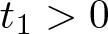 $t_1 \gt 0$ such that
 \begin{equation*} |u -\check{u} |_{\infty}\leq C\|u -\check{u} \|_{L^2(\Omega)},~t \gt t_1.\end{equation*}
We now discuss the case  $r \gt 1$. It is not difficult to see that
 \begin{equation*}-\frac{p(x,t) \frac{N}{r|\Omega|} \frac{(r-1)N}{r|\Omega|}}{|\Omega|N^{-1}}+q(x,t) \frac{(r-1)N}{r|\Omega|}=- rq(x,t) \frac{(r-1)N}{r|\Omega|} +q(x,t) \frac{(r-1)N}{r|\Omega|}=0.\end{equation*}
That is,
 \begin{equation*}(\tilde{u}, \tilde{v})=\left(\frac{N}{r|\Omega|}, \frac{(r-1)N}{r|\Omega|}\right)\end{equation*}
is an endemic  $T$-periodic solution of (1.4). This can be demonstrated through the Lyapunov functional (see, e.g., Peng and Zhao [Reference Peng and Zhao34] and Peng and Liu [Reference Peng and Liu31]). Due to the need for necessary modifications, we provide a detailed proof process: Let
 $(u(x,t),v(x,t))$ be a positive solution of (1.4) and
 \begin{equation*}E(t)=\int_\Omega \left(u-\tilde{u}\log u+v-\tilde{v}\log v\right)dx.\end{equation*}
Then, a direct computation yields that
 \begin{align*}
\frac{dE(t)}{dt}=&\tilde{u}\langle(-d_u\Delta_N)^{s_1} u\mid u^{-1}\rangle+\tilde{v}\langle(-d_v\Delta_N)^{s_2} v\mid v^{-1}\rangle\\ &+\int_\Omega \left[\left( 1-\frac{\tilde{u}}{u}\right)\left( -\frac{p(x,t) u v}{u+v}+q(x,t) v \right)+ \left( 1-\frac{\tilde{v}}{v}\right)\left(\frac{p(x,t) u v}{u+v}-q(x,t) v \right)\right] dx\\
\leq& -\int_\Omega v\left(\frac{p(x,t) u }{u+v}-q(x,t) \right) \left( \frac{\tilde{u}}{u}-\frac{\tilde{v}}{v}\right)dx=-\int_\Omega \frac{p(x,t) (u\tilde{v}-\tilde{u}v)^2}{u(u+v)(\tilde{u}+\tilde{v})} dx,
\end{align*}
here we used the fact
 \begin{equation*}\frac{1}{r}=\frac{\tilde{u}}{\tilde{u}+\tilde{v}}, ~\langle(-d \Delta_N)^s v\mid 1\rangle=0~\text{and}~\langle(-d \Delta_N)^s v\mid v^{-1}\rangle\leq0.\end{equation*}
It then follows from Theorems 2.6 and 2.9 that there exist constants  $C_\eta \gt 0$ and
 $\tilde{T}\gg1$ such that
 \begin{equation*}
\frac{dE(t)}{dt}\leq=-C_\eta\int_\Omega (u\tilde{v}-\tilde{u}v)^2 dx:=h(t) ~\text{for all}~t\geq \tilde{T}.
\end{equation*}
Again, Theorems 2.6 and 2.9 imply that  $h'(t)$ is bounded on
 $[\tilde{T},\infty)$ and
 $E(t)$ is bounded from below in
 $[\tilde{T},\infty)$. By Lemma 2.11, we have
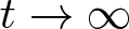
 $h(t)\rightarrow0$ as
 $t\rightarrow\infty$. Thus,
 \begin{equation}
\lim_{t\rightarrow\infty}\int_\Omega |(r-1)u(x,t)-v(x,t)|dx=0.
\end{equation}
On the other hand, by (H2) and (1.4), we have
 \begin{equation*}\frac{\partial}{\partial t}\int_\Omega (u+v)dx=\langle(-d_u\Delta_N)^{s_1} u\mid 1\rangle+\langle(-d_v\Delta_N)^{s_2} v\mid 1\rangle=0~\text{for all}~t \gt 0.\end{equation*}
This implies that
 \begin{equation} \int_\Omega (u+v)dx=N ~\text{for all}~ t\geq0.
\end{equation}
It follows from (2.23) and (2.24) that
 \begin{equation}
\lim_{t\rightarrow\infty}\int_\Omega (|u(x,t)-\tilde{u}|+| v(x,t)-\tilde{v}|)
dx=0.
\end{equation}
As shown in Theorem 2.9, given any  $w\in X_1$, we let
 $\omega(w)$ denote the omega-limit set of
 $w$ for the discrete-time semiflow
 $\{\Phi^m\}_{m\geq0}$. Observed that for any
 $\varphi=(\varphi_1,\varphi_2)\in \omega(w)$, there exists a sequence
 $m_l\rightarrow\infty$ such that
 $ \lim_{l\rightarrow\infty}\Phi^{m_l}(w)=\lim_{l\rightarrow\infty} \Psi(m_lT)(w)=\varphi$ in
 $X\times X$. Then by (2.25), and taking
 $(u(x,t), v(x,t))=[\Psi(t)w](x)$ with
 $t=m_lT$, we have
 \begin{equation*}
\int_\Omega (|\varphi_1(x)-\tilde{u}|+|\varphi_2(x)-\tilde{v}|)dx=0.
\end{equation*}
This shows that 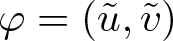 $\varphi=(\tilde{u}, \tilde{v})$. That is,
 $\omega(w)=\{(\tilde{u}, \tilde{v})\}$. Hence,
 $\lim_{t\rightarrow\infty}\Psi(t)w=(\tilde{u}, \tilde{v})$ in
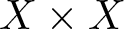 $X\times X$. This finishes the proof.
Below, we examine the stability of  $T$-periodic positive solution of
 $(1.4)$ when
 $d_u=d_v$ and
 $s_1=s_2$. We first show the alternative statements of system (2.10).
Lemma 2.13. Assume that  $d_u=d_v=d$ and
 $s_1=s_2=s$. The pair
 $(\tilde{u},\tilde{v})$ is a solution of
 $(2.10)$ if and only if it is a solution of
 \begin{equation}
\begin{cases}
u(x, t)+v(x, t)=\frac{N}{|\Omega|}, &( x, t) \in \overline{\Omega}\times\mathbb{R}, \\ v_t+(-d \Delta_N)^{s} v=[p(x, t) -q(x, t)]v-\frac{|\Omega| }{N} p(x, t)v^2, & ( x, t) \in \overline{\Omega}\times\mathbb{R}, \\ v(x, t)=v(x, t+T), & ( x, t) \in \overline{\Omega}\times\mathbb{R}.
\end{cases}
\end{equation}
Proof. If  $(\tilde{u},\tilde{v})$ is a solution of
 $(2.10)$, then there is
 \begin{equation*}
\left(\tilde{u}+\tilde{v}\right)_t+(-d \Delta_N)^{s}\left(\tilde{u}+\tilde{v}\right)=0
\end{equation*}
with  $d_u=d_v=d$ and
 $s_1=s_2=s$. Similar to the proof of Theorem 2.9, we have
 $\tilde{u}+\tilde{v}$ uniformly converges to
 $\frac{N}{|\Omega|}$ on
 $\overline{\Omega}$ as
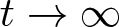 $t\rightarrow\infty$. Thus, we can see that
 \begin{equation*}
\tilde{u}(x,t)+\tilde{v}(x,t)-\frac{N}{|\Omega|}=\lim_{m\rightarrow\infty}[\tilde{u}(x,t+mT)+\tilde{v}(x,t+mT)]-\frac{N}{|\Omega|}=0 ~\text{for all}~x\in\overline{\Omega}.
\end{equation*}
Substituting  $\tilde{u}(x,t)+\tilde{v}(x,t)=\frac{N}{|\Omega|}$ into the second equation of
 $(2.10)$, we obtain (2.26).
Finally, if  $(\tilde{u},\tilde{v})$ is a solution of (2.26), then a simple calculation gives that
 \begin{equation*}
\begin{aligned}
\tilde{u}_t&= (-d \Delta_N)^{s} \tilde{v}-[p(x, t) -q(x, t)]\tilde{v}+\frac{|\Omega| }{N} p(x, t)\tilde{v}^2 \\
& =-(-d \Delta_N)^{s}\tilde{u}-\frac{p(x,t) \tilde{u} \tilde{v}}{\tilde{u}+\tilde{v}}+q(x,t) \tilde{v}, ~x \in \overline{\Omega}, ~t \in \mathbb{R}.
\end{aligned}
\end{equation*}
This shows that  $(\tilde{u},\tilde{v})$ is a solution of
 $(2.10)$, and the proof is finished.
Next, we consider the problem
 \begin{equation}
\begin{cases}u_t+(-d \Delta_N)^{s} u=u f(x, t, u), & ( x, t) \in \overline{\Omega}\times\mathbb{R}^+, \\ u(x,0)=u_0(x), & x \in \overline{\Omega},\end{cases}
\end{equation}
and
 \begin{equation}
\begin{cases}u_t+(-d \Delta_N)^{s} u=u f(x, t, u), & ( x, t) \in \overline{\Omega}\times\mathbb{R}, \\ u(x,t+T)=u( x,t), & ( x, t) \in \overline{\Omega}\times\mathbb{R},\end{cases}
\end{equation}
where  $f(x, t, u) \in C^{2 \alpha, 1}\left(\Sigma \times \mathbb{R}^{+}\right)$ and
 $f(\cdot, t+T, \cdot)=f(\cdot, t, \cdot)$ for some
 $T \gt 0$, where
 $\Sigma=\bar{\Omega}\times\mathbb{R}$ and
 $0 \lt \alpha \lt \min\{s , 1 / 2\}$,
 $f_u(t, x, u) \lt 0$ in
 $\Sigma \times(0, \infty)$ and there exists
 $M \gt 0$ such that
 $f(x, t, u) \leq 0$ for all
 $(x, t, u) \in \Sigma \times[M, \infty)$.
Proposition 2.14. Let  $u(\cdot, t; u_0)$ be a solution of
 $(2.27)$ with initial data
 $u_0 \gneq 0, \in X$. Then the following statements hold:
(i) If
$\lambda_f \lt 0$, then
$(2.28)$ has a unique periodic solution
$u^*\in Int C^+_T$, and
\begin{equation*}\|u(\cdot, t; u_0)-u^*(\cdot,t)\|_X\rightarrow 0 ~\text{as}~t\rightarrow\infty;\end{equation*}(ii) If
$\lambda_f\geq0$, then
$(2.28)$ has no periodic solution on
$ Int C^+_T$, and
\begin{equation*}\|u(\cdot, t; u_0) \|_X\rightarrow 0 ~\text{as}~t\rightarrow\infty,\end{equation*}


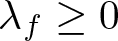


where  $\lambda_f$ is the principal eigenvalue of the periodic-parabolic eigenvalue problem
 \begin{equation*}
\begin{cases} \varphi_t+\left(-d_v\Delta_N\right)^s \varphi =f(\cdot, t,0)\varphi+\lambda\varphi, &( x, t) \in \overline{\Omega}\times\mathbb{R},\\
\varphi(x,t+T)=\varphi(x,t), & ( x, t) \in \overline{\Omega}\times\mathbb{R}.
\end{cases}
\end{equation*}
Proof. These results can be obtained by the abstract theory of monotone dynamical systems (see Section 3 of [Reference Zhao48]). As shown in Theorem 2.9, the introduction of the corresponding Poincaré map  $\Phi: \mathcal{A}^+ \rightarrow \mathcal{A}^+$, combined with the assumption conditions of
 $f$, it is easy to see that
 $\Phi: \mathcal{A}^+ \rightarrow \mathcal{A}^+$ is compact and strict subhomogeneity. Similar to the proof of [Reference Zhao48, Theorem 3.1.5], it follows from [Reference Zhao48, Theorem 2.3.4] that there exists a unique positive
 $T$-periodic solution
 $u^*$ to equation
 $(2.28)$, which is globally asymptotically stable when
 $\lambda_f \lt 0$. And
 $0$ is globally asymptotically stable when
 $\lambda_f\geq0$.
Theorem 2.15 Assume that 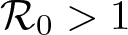 $ \mathcal{R}_0 \gt 1$,
 $d_u=d_v=d$ and
 $s_1=s_2=s$. Then
 $(2.10)$ has a unique solution
 $(\tilde{u},\tilde{v})\in\operatorname{Int} C_T^{+}$.
Proof. Since  $\mathcal{R}_0 \gt 1$, Proposition 2.1 implies that
 $\lambda_0 \lt 0$. Subsequently, it follows from Proposition 2.14 that (2.26) has a unique solution
 $\tilde{v} \in \operatorname{Int} C_T^{+}$. Observe that
 \begin{equation*}
\frac{\partial}{\partial t}\frac{N}{|\Omega|} +(-d \Delta_N)^{s} \frac{N}{|\Omega|} \gt [p(x, t)-q(x, t)]\frac{N}{|\Omega|}-\frac{|\Omega| }{N} p(x, t)\left(\frac{N}{|\Omega|}\right)^2.
\end{equation*}
By the comparison principle, we have  $\tilde{v} \leq \frac{N}{|\Omega|}$. Noting that
 $d_u=d_v=d$ and
 $s_1=s_2=s$, by Lemma 2.13, we have
 $(2.10)$ admits a unique solution
 $(\tilde{u},\tilde{v})\in\operatorname{Int} C_T^{+}$. This completes the proof.
Theorem 2.16 Suppose that  $ \mathcal{R}_0 \gt 1$,
 $d_u=d_v=d$ and
 $s_1=s_2=s$. Then the endemic T-periodic solution
 $(\tilde{u},\tilde{v})$ is globally asymptotically stable.
Proof. As in the proof of Lemma 2.13, we can obtain that
 \begin{equation*} u(x,t) + v(x,t)\rightarrow\frac{N}{|\Omega|}~\text{uniformly for}~x\in\overline{\Omega} ~\text{as}~t\rightarrow\infty,\end{equation*}
where  $(u(x,t),v(x,t))$ is global solution of
 $(1.4)$. Thus, for sufficiently small
 $\varepsilon \gt 0$, there is
 $T_\varepsilon$ such that
 $\frac{N}{|\Omega|}-\varepsilon\leq u(x,t) + v(x,t)\leq \frac{N}{|\Omega|}+\varepsilon$ for all
 $x\in\overline{\Omega}$ and
 $t\geq T_\varepsilon$. In view of Lemma 2.13, we consider the following problem
 \begin{equation}
\begin{cases}
\bar{v}^\varepsilon_t+(-d \Delta_N)^{s} \bar{v}^\varepsilon=[p(x, t) -q(x, t)]\bar{v}^\varepsilon-\frac{p(x, t)}{\frac{N}{|\Omega|}+\varepsilon }(\bar{v}^\varepsilon)^2, ~&x \in \overline{\Omega}, ~t\geq T_\varepsilon,\\
\bar{v}^\varepsilon(x,T_\varepsilon)= v (x,T_\varepsilon), ~&x \in \overline{\Omega},
\end{cases}
\end{equation}
and
 \begin{equation}
\begin{cases}
\underline{v}^\varepsilon_t+(-d \Delta_N)^{s} \underline{v}^\varepsilon=[p(x, t) -q(x, t)]\underline{v}^\varepsilon-\frac{p(x, t)}{\frac{N}{|\Omega|}-\varepsilon }(\bar{v}^\varepsilon)^2, ~&x \in \overline{\Omega}, ~t\geq T_\varepsilon,\\
\underline{v}^\varepsilon(x,T_\varepsilon)= v (x,T_\varepsilon), ~&x \in \overline{\Omega}.
\end{cases}
\end{equation}
It is not difficult to check that (2.29) and (2.30) admit a unique solution 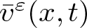 $\bar{v}^\varepsilon(x,t)$ and
 $\underline{v}^\varepsilon(x,t)$, respectively. On the other hand, we have
 $v(x,t)$ is a lower solution of (2.29) and an upper solution of (2.30) for all
 $t\geq T_\varepsilon$. Then, it follows from the comparison principle that
 \begin{equation}
\underline{v}^\varepsilon(x,t)\leq v(x,t)\leq \bar{v}^\varepsilon(x,t) ~\text{for all}~x\in\overline{\Omega} ~\text{and}~t\geq T_\varepsilon.
\end{equation}
By 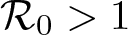 $ \mathcal{R}_0 \gt 1$ and Proposition 2.1, we have
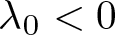 $\lambda_0 \lt 0$. It follows from Proposition 2.14 that there exist functions
 $\bar{v}^\varepsilon_*(x,t)$,
 $\underline{v}^\varepsilon_*(x,t)\in Int C^+_T$ such that
 \begin{equation}\|\bar{v}^\varepsilon(\cdot,t)-\bar{v}^\varepsilon_* (\cdot,t)\|_X\rightarrow 0 ~\text{and}~\|\underline{v}^\varepsilon(\cdot,t)-\underline{v}^\varepsilon_* (\cdot,t)\|_X\rightarrow 0 ~\text{as}~t\rightarrow\infty.\end{equation}
By the comparison principle, we obtain  $ \bar{v}^\varepsilon_* $
 $(\underline{v}^\varepsilon_*)$ is non-decreasing (non-increasing) in
 $\varepsilon$ and
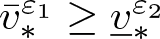 $ \bar{v}^{\varepsilon_1}_* \geq\underline{v}^{\varepsilon_2}_* $ for all
 $\varepsilon_1,\varepsilon_2 \gt 0$. Similar to the proof [Reference Lin and Wang25, Theorem 3.6], by Dini’s theorem, we have
 \begin{equation} \tilde{v}-\bar{v}^{\varepsilon}_*\rightarrow0~\text{uniformly for}~(x,t)\in\overline{\Omega}\times\mathbb{R} ~\text{as}~\varepsilon\rightarrow0,\end{equation}
and
 \begin{equation} \tilde{v}-\underline{v}^\varepsilon_*\rightarrow0~\text{uniformly for}~(x,t)\in\overline{\Omega}\times\mathbb{R} ~\text{as}~\varepsilon\rightarrow0,\end{equation}
where  $\tilde{v}$ is a solution of
 \begin{equation*}
\begin{cases}
v_t+(-d \Delta_N)^{s} v=[p(x, t) -q(x, t)]v-\frac{p(x, t)}{\frac{N}{|\Omega|} }v^2, ~&x \in \overline{\Omega}, ~t\in\mathbb{R},\\
v(x,t)= v (x,t+T), ~&x \in \overline{\Omega}. \end{cases}
\end{equation*}
It then follows from (2.31)–(2.34) that
 \begin{equation*}
\| v (\cdot,t)-\tilde{v} (\cdot,t)\|_X\rightarrow 0 ~\text{as}~t\rightarrow\infty.\end{equation*}
Noticed that  $u(x,t) + v(x,t)\rightarrow\frac{N}{|\Omega|}~\text{uniformly for}~x\in\overline{\Omega} ~\text{as}~t\rightarrow\infty$, then we have
 \begin{equation*}
\| u (\cdot,t)-\tilde{u} (\cdot,t)\|_X\rightarrow 0 ~\text{as}~t\rightarrow\infty.\end{equation*}
The proof is completed.
3. The spatial profiles of endemic periodic solutions
In this section, we study the asymptotic profiles of endemic periodic solutions of (1.4). First, we examine the spatial profiles of endemic periodic solutions of (1.4) as  $d\rightarrow 0$, where
 $d=d_u=d_v$. According to Lemma 2.13 and [Reference Zhao and Ruan47, Theorem 5.2], we have the following result.
Theorem 3.1 Suppose that  $ \mathcal{R}_0 \gt 1$,
 $d_u=d_v=d$ and
 $s_1=s_2=s$. Then endemic T-periodic solution
 $(\tilde{u},\tilde{v})$ converges to
 $(\frac{N}{|\Omega|}-\vartheta,\vartheta)$ in
 $C_T\times C_T$ as
 $d\rightarrow 0$, where
 $\vartheta$ is the unique positive solution of problem
 \begin{equation*}
\begin{cases}
\vartheta_t=[p(x, t) -q(x, t)]\vartheta-\frac{p(x, t)}{\frac{N}{|\Omega|} }\vartheta^2, ~&x \in \overline{\Omega}, ~t\in\mathbb{R},\\
\vartheta(x,t)=\vartheta(x,t+T), ~&x \in \overline{\Omega}, ~t\in\mathbb{R}. \end{cases}
\end{equation*}
We next examine the spatial profiles of endemic periodic solution  $(u, v)$ of (1.4) as
 $d_u, d_v\rightarrow+\infty$. Denote
 $\overline{w}(t)=\frac{1}{|\Omega|}\int_\Omega w(x,t)dx.$
Theorem 3.2 Suppose that 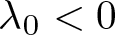 $\lambda_0 \lt 0$. Then
 $(1.4)$ admits an endemic periodic solution
 $(u, v)$ and
 $(u, v)\rightarrow (u_*, v_*)$ uniformly on
 $\overline{\Omega}\times\mathbb{R}$ as
 $d_u, d_v\rightarrow+\infty$, where
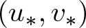 $(u_*, v_*)$ is the positive
 $T$-periodic solution of
 \begin{equation}
\begin{cases}\frac{d u_*}{d t} = -\frac{\overline{p}(t) u_* v_*}{u_*+v_*}+\overline{q}(t) v_*, & t\in\mathbb{R}, \\
\frac{d v_*}{d t} =\frac{\overline{p}(t)u_* v_*}{u_*+v_*}-\overline{q}( t) v_*, & t\in\mathbb{R}.\end{cases}
\end{equation}
Proof. Since  $\lambda_0 \lt 0$, we have
 $ \mathcal{R}_0 \gt 1$ due to Proposition 2.1. It follows from Theorem 2.9 that
 $(1.4)$ admits an endemic periodic solution
 $(u, v)$. As in the proof of Theorem 2.12, we have
 $\| u \|_X\leq \tilde{C}_1$ and
 $\| v \|_X\leq \tilde{C}_1$ for some positive constant
 $\tilde{C}_1$ and for all
 $t\geq0$. Taking the average of (2.10) over
 $ \Omega $, we have
 \begin{equation}
\begin{cases}\frac{d\overline{u}(t)}{dt}= \frac{1}{|\Omega|}\int_\Omega\left[-\frac{p(x,t) u v}{u+v}+q(x,t) v\right]dx, & t\in\mathbb{R}, \\
\frac{d\overline{v}(t)}{dt}=\frac{1}{|\Omega|}\int_\Omega\left[\frac{p(x,t)u v}{u+v}-q(x,t) v\right]dx, & t\in\mathbb{R}. \end{cases}
\end{equation}
Then by integrating (3.2) from  $0$ to
 $t$, we obtain that
 \begin{equation}
\begin{cases} \overline{u}(t)-\overline{u}(0) = \frac{1}{|\Omega|}\int_0^t\int_\Omega\left[-\frac{p(x,s) u v}{u+v}+q(x,s) v\right]dxds, \\
\overline{v}(t)-\overline{v}(0) =\frac{1}{|\Omega|}\int_0^t\int_\Omega\left[\frac{p(x,s) u v}{u+v}-q(x,s) v\right]dxds. \end{cases}
\end{equation}
Let
 \begin{equation*}F_1(x,t,u,v)=-\frac{p(x,t) u v}{u+v}+q(x,t) v, ~F_2(x,t,u,v)= \frac{p(x,t) u v}{u+v}-q(x,t) v.\end{equation*}
Multiplying the first equation of (2.10) by  $u$ and integrating over
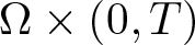 $\Omega\times(0,T)$, we have
 \begin{equation*}
\begin{aligned} \int_0^T\int_\Omega F_1(x,t,u,v)udxdt=&d_u^{s_1}\int_0^T\int_{\Omega} \int_{\Omega} K_{s_1}(x, y)[u(x,t)-u(y,t)]^2 d y d xdt\\
=&d_u^{s_1}\int_0^T\int_{\Omega} \int_{\Omega} K_{s_1}(x, y)[U(x,t)-U(y,t)]^2 d y d xdt,
\end{aligned}
\end{equation*}
where  $U(x,t)=u(x,t)-\overline{u}(t)$ and
 $U(y,t)=u(y,t)-\overline{u}(t)$. Noting that
 $\| u \|_X\leq \tilde{C}_1$ and
 $\| v \|_X\leq \tilde{C}_1$, there exists a positive constant
 $C$ such that
 \begin{equation*}\int_0^T\int_{\Omega} \int_{\Omega} K_{s_1}(x, y)[U(x,t)-U(y,t)]^2 d y d xdt\leq \frac{C}{d_u^{s_1}}.\end{equation*}
Similar to the proof of [Reference Pellacci and Verzini30, Proposition 3.1], we have
 \begin{equation*}\int_{\Omega} U^2(x,t) d x\leq C\int_{\Omega}\int_{\Omega} K_{s_1}(x, y)[U(x,t)-U(y,t)]^2 d y d x,\end{equation*}
which implies that  $\int_{\Omega} U^2(x,t) d x\leq \frac{C}{d_u^{s_1}}$. Then by Hölder inequality, it is easy to see that
 $\int_0^T\int_{\Omega} |U(x,t)| d xdt\leq \frac{C}{\sqrt{d_u^{s_1}}}$. Likewise, we have
 $\int_0^T\int_{\Omega} |V(x,t)| d xdt\leq \frac{C}{\sqrt{d_v^{s_2}}}$, where
 $V(x,t)=v(x,t)-\overline{v}(t)$. We denote
 \begin{equation*}f_i(t)=\frac{1}{|\Omega|}\int_0^t\int_\Omega
\left[F_i(x,s,u,v)-F_i(x,s,\overline{u}(s),\overline{v}(s))\right]dxds,~
i=1,2.\end{equation*}
Then, we obtain
 \begin{equation*}
\begin{cases} \overline{u}(t)-\overline{u}(0) = \frac{1}{|\Omega|}\int_0^t\int_\Omega F_1(x,s,\overline{u}(s),\overline{v}(s))dxds+f_1(t), \\
\overline{v}(t)-\overline{v}(0) =\frac{1}{|\Omega|}\int_0^t\int_\Omega F_2(x,s,\overline{u}(s),\overline{v}(s))dxds+f_2(t). \end{cases}
\end{equation*}
By the direct computation, we have
 \begin{equation*}|F_i(x,t,u,v)-F_i(x,t,\overline{u}(t),\overline{v}(t))|\leq C(|u(x,t)-\overline{u}(t)|+|v(x,t)-\overline{v}(t)|).\end{equation*}
Hence,
 \begin{equation*}
\begin{aligned} &\int_0^t\int_\Omega\left|F_i(x,t,u,v)-F_i(x,t,\overline{u}(t),\overline{v}(t))\right|dxdt\\
&\leq C\left(\int_0^t\int_{\Omega} |u(x,s)-\overline{u}(s)|d xds+\int_0^t\int_{\Omega} |v(x,s)-\overline{v}(s)|d xds\right)\\
&\leq \frac{C}{d_u^{s_1}}+\frac{C}{d_v^{s_2}}.
\end{aligned}
\end{equation*}
This shows that
 \begin{equation*}f_i(t)\rightarrow0 ~\text{uniformly on}~(0,T) ~\text{as}~ d_u, d_v\rightarrow+\infty.\end{equation*}
By (3.2), we can see that  $|\frac{d\overline{u}(t)}{dt}|, |\frac{d\overline{v}(t)}{dt}|\leq C$ for all
 $t\in\mathbb{R}$. According to the Arzelá–Ascoli theorem, there exists a sequence of
 $(u, v)$ (still denoted by
 $(u, v)$) such that
 \begin{equation*}(\overline{u}(t), \overline{v}(t))\rightarrow (u_*(t), v_*(t)) ~\text{uniformly on}~\mathbb{R} ~\text{as}~ d_u, d_v\rightarrow+\infty,\end{equation*}
where  $(u_*(t), v_*(t))$ is the positive
 $T$-periodic solution of
 \begin{equation*}
\begin{cases} u_*(t)- u_*(0) = \int_0^t\left[-\frac{\overline{p}(s) u_* v_*}{u_*+v_*}+\overline{q}(s) v_*\right]ds, & t\in\mathbb{R}, \\
v_*(t)- v_*(0) =\int_0^t\left[\frac{\overline{p}(s)u_* v_*}{u_*+v_*}-\overline{q}(s) v_*\right]ds, & t\in\mathbb{R}.\end{cases}
\end{equation*}
Below, we show that  $(U(x,t), V(x,t))\rightarrow(0,0)$ uniformly on
 $\overline{\Omega}\times\mathbb{R}$ as
 $ d_u, d_v\rightarrow+\infty$. We use a similar proof as in [Reference Zhao and Ruan47, Theorem 4.7]. For convenience, we give a brief proof here. Note that
 \begin{equation*} \left(- d_u\Delta_N\right)^{s_1} U= -\frac{p(x,t) u v}{u+v}+q(x,t) v-u_t~\text{for all}~x\in \overline{\Omega}~\text{and}~t\in\mathbb{R}.\end{equation*}
Letting  $h_{d_u}(x,t)=-\frac{p(x,t) u v}{u+v}+q(x,t) v-\overline{u}_t$, we can easily verify that
 $h_{d_u}(x,t)\in R(-\Delta_N)$, where
 $R(-\Delta_N)$ is the range of
 $-\Delta_N$. Then,
 \begin{equation*} U_t+\left(- d_u\Delta_N|_{X_1}\right)^{s_1} U= h_{d_u},~U(\cdot,t+T)=U(\cdot,t),\end{equation*}
where  $X_1=R(-\Delta_N)$. It follows from [Reference Zhao and Ruan47, Proposition 2.7] and [Reference Lunardi27, Theorem 4.4.7] that
 \begin{equation*}U(t)=\int_{-\infty}^te^{-\left(- d_u\Delta_N|_{X_1}\right)^{s_1}(t-\tau)}h_{d_u}(\tau)d\tau.\end{equation*}
It again follows from [Reference Zhao and Ruan47, Proposition 2.7] that
 \begin{equation*}\begin{aligned}\left\|U(t)\right\|_X & \leq \int_{-\infty}^t\left\|e^{-\left(- d_u\Delta_N|_{X_1}\right)^{s_1}(t-\tau)}h_{d_u}(\tau)\right\|_X d \tau \\ & \leq C \sup _{0 \leq \tau \leq T}\left\|h_{d_u}(\tau)\right\|_X \int_0^{\infty} e^{-(d_u\omega)^{s_1} \tau} d \tau \\ & =C^{\prime}(d_u\omega)^{-s_1}\end{aligned}
\end{equation*}
for some constants  $C^{\prime} \gt 0$ and
 $\omega \gt 0$. This implies that
 $U(x,t)\rightarrow0$ uniformly on
 $\overline{\Omega}\times\mathbb{R}$ as
 $d_u \rightarrow \infty$. Likewise,
 $V(x,t)\rightarrow0$ uniformly on
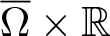 $\overline{\Omega}\times\mathbb{R}$ as
 $d_v \rightarrow \infty$ and the proof is completed.
4. Discussion
In this article, we study the SIS epidemic model with fractional diffusion and spatio-temporal heterogeneity. Using the theory of next infection operator, we define the basic reproduction number  $\mathcal{R}_0$ and systematically analyse its mathematical properties. It is important to note that in nonautonomous systems, the absence of a variational structure for
 $\mathcal{R}_0$ introduces significant technical challenges in the analysis of its properties.
Combining eigenvalue theory and uniform persistence theory, we rigourously establish  $\mathcal{R}_0$ as a threshold determining disease extinction and persistence, and prove the existence of an endemic periodic solution for system (1.4). Specifically, when
 $\mathcal{R}_0 \gt 1$, the disease persists and an endemic periodic solution exists; when
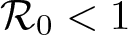 $\mathcal{R}_0 \lt 1$, the infection eventually dies out (see Theorem 2.9). Furthermore, we explore in detail how spatio-temporal heterogeneity in transmission and recovery rates influences disease dynamics.
We refer to  $\Omega$ is a high-risk domain if
 $\int_0^T\int_{\Omega} p(x,t)dxdt \gt \int_0^T\int_{\Omega}q(x,t) dxdt$,
 $\Omega$ is a low-risk domain if
 $\int_0^T\int_{\Omega} p(x,t)dxdt \lt \int_0^T\int_{\Omega}q(x,t) dxdt$. Our results show that:
• Under temporal heterogeneity, the disease consistently vanishes in low-risk regions but persists in high-risk regions;
• Under spatial heterogeneity, the disease persists in high-risk regions, while low-risk regions may not always lead to eradication if the rapid movement of infected individuals can facilitate elimination, and vice versa;
• Under spatio-temporal heterogeneity, the disease persists in high-risk domains (especially when movement is slow), and always disappears in low-risk domains (particularly when movement is sufficiently fast), as detailed in Theorem 2.10. These findings underscore that spatio-temporal heterogeneity markedly enhances epidemic persistence.
We also analyse the asymptotic behaviour of endemic periodic solutions in system (1.4). When the diffusion rates of susceptible and infected individuals are equal, controlling population movement alone is insufficient to eliminate the disease (Theorem 3.1). Without intervention, the disease will persist indefinitely (Theorem 3.2).
It should be noted that the uniqueness of the endemic periodic solution remains open in the case of 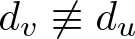 $d_v \not \equiv d_u$. Moreover, due to the absence of a parabolic Harnack inequality for fractional diffusion equations, a thorough analysis of the asymptotic profiles of these solutions is currently infeasible. In particular, their behaviour remains unknown in the following limiting scenarios:
i) as  $d_v \to 0$ with
 $d_u \gt 0$, or
 $d_v \gt 0$ with
 $d_u \to 0$;
ii) as  $d_v \to \infty$ with
 $d_u \gt 0$, or
 $d_v \gt 0$ with
 $d_u \to \infty$.
These open questions will be the focus of future research.
This study aims to clarify, through mathematical analysis of model (1.4), how long-distance human mobility and spatio-temporal environmental heterogeneity affect the spread of infectious diseases. Our work not only extends the theoretical foundations of disease transmission dynamics but may also inform the optimization of public health resource allocation and support targeted disease control strategies.
Acknowledgements
Research of W.-T. Li was partially supported by NSF of China (12531008, 12271226), NSF of Gansu Province of China (21JR7RA537), and the Fundamental Research Funds for the Central Universities (lzujbky-2022-sp07).


