2.1 Proximity voting theory and metric requirements

The theoretical foundation for spatial voting models rests on the proximity voting framework developed by Downs (Reference Downs1957) and formalized by Davis, Hinich, and Ordeshook (Reference Davis, Hinich and Ordeshook1970). Under this framework, each voter i possesses an ideal point $x_i$ in a policy space and evaluates alternatives (y) by their distance from this ideal point. For a policy located at position y, the voter’s utility follows:

(1) $$ \begin{align} U_i(y) = -d(x_i, y) + \epsilon_i, \end{align} $$

where $d(\cdot , \cdot )$ represents a distance function and $\epsilon _i$ is a random utility component. The voter prefers alternative A over alternative B when $U_i(A)> U_i(B)$ ; absent stochastic shocks, this occurs when $d(x_i,A)<d(x_i,B)$ , so A is closer to the voter’s ideal point than B. With shocks, the comparison also depends on $\epsilon _{iA}-\epsilon _{iB}$ : under $U_i(j)=-d(x_i,j)+\epsilon _{ij}$ , $U_i(A)>U_i(B)$ holds when $d(x_i,A)-d(x_i,B)<\epsilon _{iA}-\epsilon _{iB}$ .

The proximity voting framework implicitly assumes that $d(\cdot , \cdot )$ constitutes a proper distance metric. Three properties are essential for the theoretical coherence of this framework. First, symmetry requires $d(x,y) = d(y,x)$ : the ideological distance from position x to position y equals the distance from y to x. Without symmetry, the model would imply that moving from a liberal to conservative position involves a different ideological journey than moving from conservative to liberal, contradicting the reciprocal nature of ideological proximity. Second, the triangle inequality requires $d(x,y) + d(y,z) \geq d(x,z)$ for all points: the direct distance between two positions cannot exceed the sum of distances through an intermediate position. Without this property, indirect ideological paths could be shorter than direct paths, violating basic intuitions about ideological space and enabling paradoxical configurations where three positions cannot be consistently arranged along ideological dimensions. Third, positive definiteness requires $d(x,y)> 0$ for $x \neq y$ and $d(x,x) = 0$ : distinct positions must be separated by positive distance, while a position’s distance from itself is zero. Without this property, distinct ideological positions could be indistinguishable, rendering the spatial representation meaningless.

These metric properties are not merely mathematical conveniences—they are fundamental to the substantive interpretation of proximity voting. Consider the triangle inequality: if legislator A has an ideal point close to position x, and position x is close to position y, the triangle inequality guarantees that legislator A cannot be arbitrarily distant from position y. This transitive consistency underlies claims about coalition formation: if moderate Democrats are close to centrist positions, and centrist positions are close to moderate Republicans, then moderate Democrats and moderate Republicans must be relatively proximate, enabling bipartisan coalitions. Without the triangle inequality, such transitive reasoning fails—proximity becomes intransitive, and the spatial metaphor loses coherent meaning.

Given these metric requirements, we now examine the utility formulations commonly used in spatial voting models, focusing on whether quadratic and Gaussian utility preserve the triangle inequality required for a metric notion of ideological proximity. This discussion concerns the theoretical utility formulation; issues related to how ideal point models are represented and estimated in practice are addressed separately in Section 3.

2.2 The triangle inequality and its violation in conventional methods

A distance function $d: \mathcal {X} \times \mathcal {X} \rightarrow \mathbb {R}_+$ defines a metric space if it satisfies four properties: (1) non-negativity: $d(x,y) \geq 0$ with equality if and only if $x=y$ ; (2) symmetry: $d(x,y) = d(y,x)$ ; (3) triangle inequality: $d(x,y) + d(y,z) \geq d(x,z)$ for all $x,y,z \in \mathcal {X}$ ; and (4) identity of indiscernibles. The triangle inequality is particularly important: it ensures that distances are additive, comparable and transitively consistent. Without this property, distance comparisons become difficult to interpret—for example, it becomes unclear whether one pair is “twice as distant” as another or whether distance-based clustering methods that assume metric structure are appropriate.

In terms of their theoretical specification, conventional spatial voting models typically employ utility formulations based on squared distance. In BIRT (Clinton et al. Reference Clinton, Jackman and Rivers2004), legislators maximize quadratic utility derived from proximity voting: for each roll-call j presenting a binary choice between “Yea” position $\zeta _j$ and “Nay” position $\psi _j$ , legislator i with ideal point $x_i$ votes “Yea” when

$$ \begin{align*}-\lVert x_i - \zeta_j \rVert^2 + \eta_{ij}> -\lVert x_i - \psi_j \rVert^2 + \nu_{ij}.\end{align*} $$

This formulation implies that utility decreases with the squared Euclidean distance between the legislator and policy positions. However, squared distance itself does not satisfy the triangle inequality and therefore does not define a metric distance. Consider $d_Q(x,y) = (x-y)^2$ in one dimension. The triangle inequality requires $(x-y)^2 + (y-z)^2 \geq (x-z)^2$ . Expanding $(x-z)^2 = [(x-y) + (y-z)]^2 = (x-y)^2 + 2(x-y)(y-z) + (y-z)^2$ , the inequality reduces to $2(x-y)(y-z) \leq 0$ . This condition holds when $(x-y)$ and $(y-z)$ have opposite signs (or when one of them is zero), but fails when they have the same sign.

In NOMINATE (Poole and Rosenthal Reference Poole and Rosenthal2007), spatial voting is often motivated using Gaussian utility:

$$ \begin{align*}U_i(\zeta_j) = \beta\ \exp\{-\frac{1}{2}\sum_k w_k^2(x_{ik} - \zeta_{jk})^2\}.\end{align*} $$

The exponential transformation of squared distances alters the geometry implied by spatial proximity. To illustrate, consider the one-dimensional quantity $d_G(x,y) = -\exp \{-\tfrac {1}{2}(x-y)^2\}$ . For three points $x=3$ , $y=3$ and $z=-1$ , we obtain

$$ \begin{align*}d_G(x,y) = -\exp\{0\} = -1, \quad d_G(y,z) = -\exp\{-8\}, \quad d_G(x,z) = -\exp\{-8\}.\end{align*} $$

The triangle inequality would require $d_G(x,y) + d_G(y,z) \geq d_G(x,z)$ , but

$$ \begin{align*}-1 - \exp\{-8\} < -\exp\{-8\},\end{align*} $$

so the inequality is violated. Thus, the geometry implied by Gaussian utility does not correspond to a metric distance.

Such configurations can arise when legislators are presented with policy alternatives that move policy in the same ideological direction but by different magnitudes. For example, suppose a legislator’s ideal point lies near the status quo, and two amendments propose more moderate and more extreme versions of a policy change in the same direction. In this situation, the legislator, the moderate amendment and the more extreme amendment lie along a single ideological line but at increasing distances from one another. Under squared-distance comparisons, this configuration can violate the triangle inequality even in a one-dimensional policy space.

While such violations can arise even in one-dimensional settings, their practical importance depends on the structure of the voting environment. In highly structured left–right settings, where alternatives are consistently ordered along a single ideological dimension, conventional models can recover the dominant partisan structure reasonably well. However, violations become more substantively relevant when the voting environment departs from this simple ordering—for instance, when both alternatives lie on the same ideological side (e.g., two competing left-leaning amendments), when procedural votes place both positions far from most ideal points or when a unidimensional model is fit to an inherently multi-dimensional space.

When such configurations occur, the resulting non-metric geometry can complicate geometric interpretations of legislators’ positions in the ideological space. For example, researchers often summarize party cohesion using the dispersion of legislators’ positions within a party. If the underlying distance representation is non-metric, differences in dispersion may partly reflect how the utility formulation scales distances across the ideological space rather than only differences in voting cohesion. Similar considerations arise when clustering legislator positions to identify factions or when comparing ideological separations across policy dimensions. The concern we raise is structural rather than empirical: a non-metric distance function lacks the geometric guarantees—transitivity of separations, additivity through intermediate points and cross-dimensional comparability—that underlie distance-based inference, regardless of how often violations are realized in a given dataset.

2.3 Euclidean distance as a metric

Euclidean distance $d_E(x,y) = \sqrt {\sum _{k=1}^K (x_k - y_k)^2}$ satisfies the triangle inequality and defines a proper metric space. The proof follows directly from the Cauchy–Schwarz inequality: for any three points ${x, y, z \in \mathbb {R}^K}$ , squaring $d_E(x,y) + d_E(y,z) \geq d_E(x,z)$ and expanding yields $d_E(x,y)d_E(y,z) \geq \sum _k (x_k-y_k)(y_k-z_k)$ , which holds because $|\sum _k (x_k-y_k)(y_k-z_k)| \leq \sqrt {\sum _k (x_k-y_k)^2}\sqrt {\sum _k (y_k-z_k)^2} = d_E(x,y)d_E(y,z)$ by the Cauchy–Schwarz inequality.

This metric property has direct implications for legislative analysis. First, distances become cardinally interpretable: if $d_E(z_A, z_B) = 2 d_E(z_C, z_D)$ , legislators A and B are genuinely twice as ideologically separated as C and D in their voting behavior. Second, distances become comparable across dimensions: we can meaningfully ask whether the first or second dimension generates greater polarization by comparing distance statistics, because the metric structure allows these comparisons to be interpreted directly in terms of spatial separation in the latent space. Third, clustering methods that assume metric distances—k-means, hierarchical clustering and silhouette analysis—can be applied in a geometrically coherent way because pairwise distances satisfy the triangle inequality. For example, the silhouette coefficient measures cluster quality by comparing mean within-cluster distances to mean nearest-cluster distances, a computation that requires pairwise distances to be metrically consistent. Fourth, the geometric interpretation aligns with mathematical properties: points that appear close in two-dimensional visualizations genuinely vote similarly, and spatial neighborhoods correspond to actual voting coalitions rather than distortions induced by non-metric utility functions.

At the same time, metric embeddings are not free from scaling artifacts. As in other low-dimensional embedding methods such as multidimensional scaling or spectral embeddings, geometric patterns such as curvature or horseshoe structures may arise when complex preference structures are approximated in a limited number of dimensions (e.g., Diaconis, Goel, and Holmes Reference Diaconis, Goel and Holmes2008). These limitations reflect the challenge of representing high-dimensional preference structures in a small number of spatial dimensions rather than a failure of the metric formulation itself.

3.1 Bipartite network framework

Roll-call voting data constitute a bipartite network linking legislators to bills through binary votes (excluding abstentions). Formally, let $G=(L,B,E)$ denote a bipartite graph, where $L=\{1,\ldots ,N\}$ represents legislators and $B=\{1,\ldots ,M\}$ represents bills. An edge between legislator i and bill j is represented by the adjacency variable $y_{ij}$ , where

$$\begin{align*}y_{ij} = \begin{cases} 1 & \text{if legislator } i \text{ votes "yea" on bill } j, \\ 0 & \text{otherwise}. \end{cases} \end{align*}$$

The resulting $N \times M$ adjacency matrix $Y=(y_{ij})$ corresponds directly to the roll-call voting matrix commonly analyzed in ideal point estimation. This representation treats roll-call voting as an affiliation network linking legislators to bills. Alternative network constructions are possible—for example, including status quo nodes or using a doubled network that treats “yea” and “nay” as separate edge types. We adopt the legislator–bill affiliation network because it corresponds directly to the observed roll-call matrix and enables joint embedding of legislators and bills in a shared latent policy space. In our formulation, nay votes are already incorporated through the complement of the modeled probability, so a doubled network would increase complexity without adding information.

Latent variable models provide a natural framework for representing relational data of this type. In the latent space approach to network modeling (Hoff Reference Hoff2007; Hoff, Raftery, and Handcock Reference Hoff, Raftery and Handcock2002), nodes are assigned positions in a low-dimensional space, and the probability of an edge depends on the relationship between their latent positions. Adapting this idea to the legislator–bill setting, let $z_i \in \mathbb {R}^K$ denote the latent position of legislator i and $w_j \in \mathbb {R}^K$ the latent position of bill j. The probability of a “Yea” vote depends on their spatial relationship:

(2) $$ \begin{align} g\left(\Pr(y_{ij}=1 \mid z_i, w_j)\right) = \mu + \alpha(z_i, w_j), \end{align} $$

where $g(\cdot )$ denotes a link function and $\alpha (z_i, w_j)$ specifies how latent positions determine voting propensity. Three canonical specifications exist. The latent class model (LCM; Airoldi et al. Reference Airoldi, Blei, Fienberg and Xing2008; Holland, Laskey, and Leinhardt Reference Holland, Laskey and Leinhardt1983; Miller, Jordan, and Griffiths Reference Miller, Jordan, Griffiths, Bengio, Schuurmans, Lafferty, Williams and Culotta2009; Mørup, Schmidt, and Hansen Reference Mørup, Schmidt and Hansen2011; Nowicki and Snijders Reference Nowicki and Snijders2001; Palla, Knowles, and Ghahramani Reference Palla, Knowles and Ghahramani2012; Zhou Reference Zhou2015) and stochastic blockmodel (SBM; Airoldi et al. Reference Airoldi, Blei, Fienberg and Xing2008; Daudin, Picard, and Robin Reference Daudin, Picard and Robin2008; Holland et al. Reference Holland, Laskey and Leinhardt1983; Karrer and Newman Reference Karrer and Newman2011; Nowicki and Snijders Reference Nowicki and Snijders2001; Vu, Hunter, and Schweinberger Reference Vu, Hunter and Schweinberger2013) set $\alpha (z_i, w_j) = m_{u_i, v_j}$ for discrete group memberships $u_i, v_j \in \{1,\ldots ,K\}$ and interaction matrix $M = (m_{k\ell })$ , capturing stochastic equivalence where legislators in the same class vote identically. The latent eigenmodel (Hoff Reference Hoff2007; Hoff Reference Hoff2009; Hoff Reference Hoff2021; Li, Yeung, and Zhang Reference Li, Yeung and Zhang2011; Young and Scheinerman Reference Young, Scheinerman, Bonato and Chung2007) defines $\alpha (z_i, w_j) = z_i^{\top }\Lambda w_j$ for a diagonal matrix $\Lambda $ , representing voting through weighted inner products that extend principal component analysis to binary data. The latent distance model (Handcock, Raftery, and Tantrum Reference Handcock, Raftery and Tantrum2007; Hoff Reference Hoff2007; Hoff et al. Reference Hoff, Raftery and Handcock2002; Kemp et al. Reference Kemp, Tenenbaum, Griffiths, Yamada and Ueda2006; Krivitsky and Handcock Reference Krivitsky and Handcock2008; Raftery et al. Reference Raftery, Niu, Hoff and Yeung2012; Schweinberger and Snijders Reference Schweinberger and Snijders2003; Sewell and Chen Reference Sewell and Chen2015; Smith, Asta, and Calder Reference Smith, Asta and Calder2019) specifies $\alpha (z_i, w_j) = -\gamma \lVert z_i - w_j \rVert $ , where voting probability decreases monotonically with spatial separation, operationalizing homophily through spatial proximity.

Conventional ideal point methods, however, treat this bipartite structure asymmetrically: legislators receive interpretable spatial positions (ideal points), while bills serve primarily as instruments for scaling, with bill parameters $(\alpha _j, \beta _j)$ estimated but not embedded in the same space. In BIRT (Clinton et al. Reference Clinton, Jackman and Rivers2004), the probability of a “Yea” vote is typically written as

$$\begin{align*}\text{logit}\,P(y_{ij}=1) = \alpha_j + \beta_j^{\top} x_i , \end{align*}$$

where $x_i$ denotes the legislator’s ideal point and $(\alpha _j,\beta _j)$ are bill parameters. Although this formulation is motivated by spatial proximity voting, the statistical representation of the model reduces to an interaction between legislator positions and bill loadings through the inner product $\beta _j^{\top } x_i$ . As a result, bills are not represented as identifiable spatial locations comparable to legislators. The reparameterization from spatial bill positions $(\zeta _j, \psi _j)$ to discrimination parameters $(\alpha _j, \beta _j)$ is many-to-one—entirely different bill locations generate identical parameters—making bills difficult to interpret as spatial entities (Nakis et al. Reference Nakis, Holm, Fiehn and Mørup2025; Shin et al. Reference Shin, Lim and Park2024). In addition, the model does not include a separate legislator-specific intercept capturing baseline voting propensity; instead, variation across legislators is represented solely through their spatial positions.

Jeon et al. (Reference Jeon, Jin, Schweinberger and Baugh2021) introduced the LSIRM for educational testing, embedding respondents and items in a shared latent space. This symmetric framework applies naturally to roll-call voting data, where legislators and bills form the two modes of a bipartite system. It is also flexible with respect to the geometric operator governing interactions: Jeon et al. (Reference Jeon, Jin, Schweinberger and Baugh2021) consider both an inner-product specification, analogous to the latent eigenmodel (Hoff Reference Hoff2007), and a distance-based specification. The former captures directional alignment through $z_i^{\top } w_j$ , whereas the latter captures spatial proximity through Euclidean distance. In this article, we adopt the Euclidean specification.

Distance-based specifications have been applied to political networks in two contexts, though with different formulations and objectives than ours. Barberá (Reference Barberá2015) employed a latent space model to estimate ideal points from Twitter following patterns, treating the data as a bipartite network where users choose whether to follow political actors. Users i and political actors j are embedded in a shared latent space, with following probability modeled as $P(y_{ij}=1) = f(\phi - \gamma \lVert \theta _i - \beta _j \rVert ^2)$ , where $\lVert \theta _i - \beta _j \rVert ^2$ represents squared Euclidean distance. However, as discussed in Section 2, this squared distance formulation does not satisfy the triangle inequality and therefore produces a non-metric spatial representation.

Taken together, these approaches reveal two limitations in the spatial analysis of roll-call voting. First, in conventional ideal point models, bills are treated primarily as scaling instruments with parameters that do not correspond to identifiable spatial locations. Second, distance-based specifications used in political network models typically rely on squared Euclidean distance, which—as discussed in Section 2—does not satisfy the triangle inequality and therefore produces a non-metric representation of ideological space. In the next section, we introduce a Euclidean latent space formulation for roll-call voting that embeds legislators and bills in a shared space using Euclidean distance and allows direct comparison with inner-product-based representations.

3.2 Euclidean distance specification

We specify voting probability through Euclidean distance in a bipartite network framework. For legislator i with latent position $z_i \in \mathbb {R}^K$ and bill j with latent position $w_j \in \mathbb {R}^K$ :

(3) $$ \begin{align} \text{logit}(P(y_{ij} = 1 \mid \theta_i, \beta_j, \gamma, z_i, w_j)) = \theta_i + \beta_j - \gamma \lVert z_i - w_j \rVert, \end{align} $$

where $\theta _i$ captures legislator i’s baseline propensity to vote “Yea,” $\beta _j$ represents bill j’s baseline popularity or controversy, and $\gamma> 0$ governs the strength of proximity effects. The Euclidean distance is ${\lVert z_i - w_j \rVert = \sqrt {\sum _{k=1}^K (z_{ik} - w_{jk})^2}}$ . The probability of a “Yea” vote increases with legislator propensity $\theta _i$ and bill popularity $\beta _j$ , but decreases with spatial distance $\lVert z_i - w_j \rVert $ . This formulation directly implements proximity voting (Davis et al. Reference Davis, Hinich and Ordeshook1970; Downs Reference Downs1957): legislators support bills near their ideal points, with support declining monotonically as separation increases.

For comparison, an inner-product LSIRM can be written as

(4) $$ \begin{align} \text{logit}(P(y_{ij} = 1 \mid \theta_i, \beta_j, z_i, w_j)) = \theta_i + \beta_j + z_i^{\top} w_j, \end{align} $$

which replaces the distance-based interaction with a bilinear form while preserving the same intercept structure.

The baseline parameters $\theta _i$ and $\beta _j$ play distinct roles from those in BIRT. In BIRT, bill positions are not separately identified such that $\alpha _j$ can be interpreted as a baseline level of support, and the model includes no legislator-specific intercept term. In our specification, $\beta _j$ measures only the baseline tendency for legislators to support bill j averaging over all spatial locations—a pure “how popular is this bill” parameter separable from its ideological location $w_j$ . Similarly, $\theta _i$ measures legislator i’s general tendency to vote “Yea” independent of ideological proximity—some legislators vote “Yea” frequently (high $\theta _i$ ) while others vote “Nay” frequently (low $\theta _i$ ) for reasons orthogonal to spatial positioning. This separation between baseline propensities and spatial structure, which is similar to the degree correction in network science literature (Fortunato Reference Fortunato2010), clarifies interpretation: if legislator i supports bill j, we can determine whether this reflects high baseline propensity ( $\theta _i$ or $\beta _j$ large), ideological proximity ( $\lVert z_i - w_j \rVert $ small), or both.

The parameter $\gamma $ quantifies the strength of spatial proximity relative to baseline propensities. Large $\gamma $ indicates voting is primarily distance-determined—legislators vote almost exclusively for nearby bills regardless of baseline propensities—while small $\gamma $ suggests the dominance of baseline propensities, a spatial structure playing a secondary role. This provides diagnostic information about legislative organization: chambers with strong, stable party or factional discipline exhibit larger $\gamma $ (tight clustering with sharp spatial boundaries), whereas fragmented or weakly organized chambers exhibit smaller $\gamma $ (diffuse positioning where baseline propensities matter more than ideological location). Our simulation studies demonstrate that $\hat {\gamma }$ responds predictably to known levels of coalition cohesion, increasing when within-group homogeneity strengthens and decreasing when independent voting attenuates the distance signal.

Inner-product models, including BIRT, measure affinity through directional alignment rather than spatial proximity, so geometric closeness does not necessarily imply a higher tie probability. As noted in the latentnet documentation, actors that are closer in a clustering sense need not have higher expected tie values (Krivitsky et al. Reference Krivitsky, Handcock, Raftery and Hoff2009). More generally, as shown by Hoff (Reference Hoff2007), inner-product formulations are representationally more flexible, which can be advantageous in networks characterized by directional equivalence or heterogeneous connectivity patterns.

By contrast, Euclidean distance models impose a stricter geometric interpretation in which spatial proximity directly governs interaction probability. This yields embeddings that are less sensitive to scale artifacts and limits the influence of unusually prominent units, such as procedural hub bills or omnibus measures. In homophilous settings such as legislative voting, the resulting geometry aligns clustering structure more closely with proximity in the latent space. Consistent with this intuition, Nakis et al. (Reference Nakis, Holm, Fiehn and Mørup2025) show that Euclidean representations can often achieve comparable structural fit with equal or lower latent dimensionality than inner-product formulations.

The bipartite embedding provides three interpretive advantages over conventional methods by locating legislators and bills in a shared latent space. Legislator-to-legislator distances reveal ideological similarity, bill-to-bill distances identify policy clustering and legislator–bill distances clarify coalition structure through spatial proximity, including the placement of cross-party bridge bills between cooperating factions. This joint embedding enables interpretation through bill locations as anchors: instead of asking “what does dimension 2 mean?”, we can observe “which bills define dimension 2?” and infer substantive meaning from the specific legislation that separates high from low values.

3.3 Full conditionals and estimation

We estimate parameters via Markov chain Monte Carlo (MCMC) sampling with the Gibbs sampling and the Metropolis–Hastings algorithm with the following prior specifications:

(5) $$ \begin{align} \begin{aligned} \theta_i &\sim N(0, \sigma_{\theta}^2), \\ \beta_j &\sim N(0, \sigma_{\beta}^2),\\ \sigma_{\theta}^2 &\sim \text{Inv-Gamma}(a_{\sigma},b_{\sigma}),\\ z_i &\sim \text{MVN}_K(\mathbf{0}, \mathbf{I}_K), \\ w_j &\sim \text{MVN}_K(\mathbf{0}, \mathbf{I}_K), \\ \log{\gamma} &\sim N(\mu_{\gamma}, \sigma_{\gamma}^2). \end{aligned} \end{align} $$

The overall scale of the latent space is regularized through the prior specification $z_i \sim \text {MVN}_K(\mathbf {0}, \mathbf {I}_K)$ and $w_j \sim \text {MVN}_K(\mathbf {0}, \mathbf {I}_K)$ . Because the likelihood depends on the Euclidean distance $\lVert z_i - w_j \rVert $ , it is invariant to joint rescaling of the latent positions and the distance coefficient $\gamma $ . The prior therefore constrains the scale of the latent space, allowing $\gamma $ to be interpreted as the strength of distance-based voting relative to this normalization.

Then, the joint posterior density of the model is given as

(6) $$ \begin{align} \begin{aligned} \pi(\boldsymbol{\beta}, \boldsymbol{\theta}, \gamma, \mathbf{Z}, \mathbf{W} \mid \mathbf{Y}) &\propto \prod_{i=1}^{N}\prod_{j=1}^{P}P(Y_{ij}=y_{ij} \mid \theta_i, \beta_j, \gamma, z_i, w_j) \\&\quad \times \pi(\gamma) \prod_{j=1}^{P}\pi(\beta_j) \prod_{i=1}^{N}\pi(\theta_i) \prod_{i=1}^{N}\pi(z_i) \prod_{j=1}^{P}\pi(w_j). \end{aligned} \end{align} $$

The priors and the following posterior distribution can be expressed in Equations (5) and (6). This posterior kernel cannot be expressed with standard distribution, so the exact posterior density cannot be calculated and a Gibbs sampler is used to sample each parameter sequentially from their conditional density. Specifically, because each conditional kernel may not be expressed as a standard distribution form, Metropolis–Hastings within Gibbs sampler is used. Furthermore, for the generalized case with missing data, the imputed value for the non-respondent pair can be sampled with the logistic formula at the start of each Gibbs sampler step:

$$ \begin{align*} \begin{aligned} \pi(\theta_i) &\propto \Bigg[\prod_{i=1}^{N}\prod_{j=1}^{P}P(Y_{ij}=y_{ij} \mid \theta_i, \beta_j, \gamma, z_i, w_j)\Bigg] \times \big[N_{\theta_i}(0, \sigma_{\theta}^2) \big]\\ \pi(\beta_j) &\propto \Bigg[\prod_{i=1}^{N}\prod_{j=1}^{P}P(Y_{ij}=y_{ij} \mid \theta_i, \beta_j, \gamma, z_i, w_j)\Bigg] \times \big[N_{\beta_j}(0, \sigma_{\beta}^2) \big]\\ \pi(\log \gamma) &\propto \Bigg[\prod_{i=1}^{N}\prod_{j=1}^{P}P(Y_{ij}=y_{ij} \mid \theta_i, \beta_j, \gamma, z_i, w_j)\Bigg] \times \big[N(\mu_{\gamma}, \sigma_{\gamma}^2)]\\ \pi(z_i) &\propto \Bigg[\prod_{i=1}^{N}\prod_{j=1}^{P}P(Y_{ij}=y_{ij} \mid \theta_i, \beta_j, \gamma, z_i, w_j)\Bigg] \times \big[\text{MVN}_{K, z_i}(\mathbf{0}, \mathbf{I}_K) \big] \end{aligned} \end{align*} $$

$$ \begin{align*} \begin{aligned} \pi(w_j) &\propto \Bigg[\prod_{i=1}^{N}\prod_{j=1}^{P}P(Y_{ij}=y_{ij} \mid \theta_i, \beta_j, \gamma, z_i, w_j)\Bigg] \times \big[\text{MVN}_{K, w_j}(\mathbf{0}, \mathbf{I}_k) \big]\\ \pi(\sigma_{\theta}) &\propto \text{Inv-Gamma}\Bigg(\bigg(\frac{N}{2}+a_{\sigma}\bigg),\frac{1}{2}\sum_{i=1}^{N}{\theta}_i^2 + b_{\sigma}\bigg). \end{aligned} \end{align*} $$

Like conventional ideal-point estimators, Euclidean LSIRM inherits rotational, reflective and translational indeterminacies: for any orthogonal matrix Q and vector c, the transformed configuration $(Qz_i + c,\; Qw_j + c)$ produces identical probabilities. Because we do not fix the positions of any legislators or bills, the absolute orientation and location of the latent space are not identified. Specifically, after obtaining posterior samples from the MCMC algorithm, we apply a Procrustes transformation (Gower Reference Gower1975) to align each sampled configuration to a reference configuration selected as the draw with the highest posterior density (Friel et al. Reference Friel, Rastelli, Wyse and Raftery2016). This post-processing removes rotational, reflective and translational indeterminacies while preserving pairwise distances among legislators and bills.Footnote ¹

4.1 Agenda sweep

Each party contains three factions (180 legislators total). We varied the share of partisan bills from 30% to 50%, with the remainder being faction-specific bills.

At both agenda compositions, BIRT and the inner-product LSIRM largely collapse factional structure, merging within-party factions into roughly three visible groups in the representative embedding (Figure 2). Euclidean LSIRM, by contrast, separates all six factions into distinct clusters. As the share of partisan bills falls from 50% to 30%, factional signals strengthen and the performance gap widens: Euclidean LSIRM’s mean silhouette increases from $0.624$ ( $SD = 0.081$ ) to $0.723$ ( $SD = 0.016$ ), while BIRT remains low ( $0.164$ – $0.172$ ) and the inner-product LSIRM shows similarly weak separation ( $0.188$ – $0.190$ ).

Figure 2

Faction recovery under shifting legislative agendas. Colors and markers denote six true factions: two parties, each containing three internal factions (180 legislators total, 30 per faction). Top row: 50% partisan bills; bottom row: 30% partisan bills. Euclidean LSIRM recovers all six factions as distinct clusters across both conditions, whereas BIRT and inner-product LSIRM collapse within-party factions into roughly three visible groups, failing to distinguish factional structure from party membership.

Figure 2. Long description

The figure consists of six panels arranged in two rows of three.

Top Row (50% partisan bills):

* Panel a, B I R T: Shows three primary clusters. Two blue-toned clusters are tightly packed in the upper-left quadrant, and one red-toned cluster is in the lower-right quadrant.

* Panel b, Inner-product L S I R M: Displays three distinct groups. A blue cluster is in the upper-left, while two red-toned clusters are separated in the lower-right quadrant.

* Panel c, Euclidean L S I R M: Shows six distinct, widely separated clusters. Three red-toned clusters are on the left side and three blue-toned clusters are on the right side of the y-axis.

Bottom Row (30% partisan bills):

* Panel d, B I R T: Similar to panel a, it shows three main groups. One blue cluster is in the lower-left, and two red-toned clusters are in the upper-right.

* Panel e, Inner-product L S I R M: Shows three groups. Two red-toned clusters are in the lower-left, and one blue cluster is in the upper-right.

* Panel f, Euclidean L S I R M: Shows six distinct clusters arranged vertically. Three red-toned clusters are positioned in the upper half of the plot, and three blue-toned clusters are positioned in the lower half, with clear spatial gaps between all six groups.

4.2 Cross-party coalitions

We introduced unequal faction sizes (70 vs. 10 legislators per faction) and two types of bridge bills: Bridge-A supported by majority factions from both parties (L1 and C1), and Bridge-B supported by minority factions (L2 and C2). This design tests whether the model can represent overlapping coalitions that transcend party lines. Additional configurations and extended results, including simulations incorporating faction bills, appear in the Supplementary Material (Section 1.3.2).

In the majority consensus scenario (Figure 3), Euclidean LSIRM correctly draws the allied majority factions closer together near the inter-party boundary, with Bridge-A bills positioned between them. Both BIRT and the inner-product LSIRM fail to represent this structure—distances between allied cross-party legislators are no shorter than distances between ideological opponents, obscuring the coalition structure in the latent space.

Figure 3

Cross-party majority coalition recovery. Two parties (Liberal: blue/purple; Conservative: red/pink) each split into a majority faction (L1, C1: 70 legislators) and a minority faction (L2, C2: 10 legislators). Bridge-A bills (gray triangles) are supported jointly by the two majority factions across party lines. Legislators are colored by party and shaped by faction (L1: blue squares, L2: purple triangles, C1: red circles and C2: pink crosses). Euclidean LSIRM correctly positions allied majority factions near the inter-party boundary with Bridge-A bills between them; BIRT and inner-product LSIRM fail to capture this cross-party coalition structure.

Figure 3. Long description

A three-panel scatter plot series on a grid.

Panel a, labeled B I R T, shows two distinct, widely separated clusters. On the left, blue squares L 1 and purple diamonds L 2 are grouped together near x equals negative 0.5. On the right, red triangles C 1 and pink crosses C 2 are grouped near x equals 0.5.

Panel b, labeled Inner-product L S I R M, shows four isolated clusters. Purple diamonds L 2 are in the far bottom-left. Blue squares L 1 are in the bottom-center. Red triangles C 1 are in the center-right. Pink crosses C 2 are at the top-center.

Panel c, labeled Euclidean L S I R M, shows a different structural arrangement. On the left, blue squares L 1 and purple diamonds L 2 form a vertical cluster near x equals negative 1. On the right, red triangles C 1 and pink crosses C 2 form a cluster near x equals 1.5. Crucially, gray triangles representing Bridge-A bills are positioned in the center space between the two party clusters, specifically concentrated between the L 1 and C 1 majority factions, indicating a recovered cross-party coalition.

In the ends-against-the-middle scenario (Duck-Mayr and Montgomery Reference Duck-Mayr and Montgomery2023), the two inner-product specifications—BIRT and the inner-product LSIRM—produce embeddings that stretch legislators along a pronounced secondary axis (Figure 4). This elongated geometry spreads factions along a single direction in the latent space.

Figure 4

Cross-party minority coalition recovery: Ends-against-the-middle scenario. Bridge-B bills (gray triangles) are supported jointly by the two minority factions (L2, C2: 10 legislators each) across party lines, while majority factions (L1, C1: 70 legislators each) oppose. Legislators are colored by party and shaped by faction (L1: blue squares, L2: purple triangles, C1: red circles and C2: pink crosses). Euclidean LSIRM draws the minority factions toward each other with Bridge-B bills positioned near this pairing, preserving interpretable proximity between legislators and the bills structuring their coalition. BIRT and inner-product LSIRM instead stretch legislators along a pronounced secondary axis, obscuring the minority coalition.

Figure 4. Long description

The figure consists of three panels labeled a, b, and c, each showing a scatter plot on a grid with axes ranging from -2 to 2.

* Panel a, B I R T. Data points are stretched vertically. Blue squares L 1 and purple triangles L 2 form a vertical column on the left around x equals -1. Red circles C 1 and pink crosses C 2 form a vertical column on the right around x equals 1. The minority factions L 2 and C 2 are at the top and bottom extremes of their respective columns.

* Panel b, Inner-product L S I R M. Data points are stretched along a secondary axis. Red circles C 1 are clustered at the top center. Blue squares L 1 are at the bottom left. Pink crosses C 2 are at the far right, and purple triangles L 2 are at the bottom right. The minority factions are widely separated.

* Panel c, Euclidean L S I R M. This plot shows a different clustering. Red circles C 1 are clustered on the left around x equals -1.5. Blue squares L 1 are clustered on the right around x equals 1.5. Crucially, the minority factions, purple triangles L 2 and pink crosses C 2, are pulled toward the center and each other. Gray triangles representing Bridge-B bills are positioned in the center gap between the two main party clusters, specifically concentrated near the L 2 and C 2 minority factions.

The Euclidean LSIRM instead organizes legislators according to spatial proximity. As a result, the two minority factions are drawn toward one another while the majority blocs remain separated. This configuration places Bridge-B bills between the opposing minority factions and preserves interpretable distances between legislators and the bills that structure their voting behavior.

5.1 Data and context

We apply Euclidean LSIRM to roll-call votes from the 118th U.S. House, obtained from Voteview (Lewis et al. Reference Lewis, Poole, Rosenthal, Boche, Rudkin and Sonnet2025). Following standard practice, we excluded lopsided votes (overwhelming majorities) that provide little ideological information, yielding 1,225 informative roll-calls across 451 unique legislators (accounting for vacancies and replacements). This chamber provides a stringent test: extreme partisan polarization (the most conservative Democrat remains left of the most moderate Republican) yet well-documented intra-party factions—the progressive “Squad” (approximately 8 members) among Democrats and the House Freedom Caucus (approximately 22 members) among Republicans. These factions, though numerically small, exert disproportionate influence on leadership contests and agenda setting, making their accurate identification substantively important. We ran five independent MCMC chains and assessed convergence using overlaid trace plots and scale reduction diagnostics (see Section 2.1 of the Supplementary Material), which indicate satisfactory mixing and stationarity. As the latent space is invariant to rigid transformations, coordinates are not directly comparable across chains; visualizations therefore use posterior means from the first converged chain.

5.2 Legislator positions and faction recovery

Figure 5 displays two-dimensional embeddings from Euclidean LSIRM and BIRT. Both methods recover clear party separation on the primary (horizontal) dimension, with Democrats left and Republicans right. However, the secondary dimension reveals striking differences. Euclidean LSIRM differentiates factions: Freedom Caucus members (e.g., Andy Biggs and Paul Gosar) occupy far-right positions with distinctly negative second-dimension coordinates, separating them from mainstream Republicans, while Squad members (e.g., Ilhan Omar and Alexandria Ocasio-Cortez) appear below with slightly negative values, distinguishing them from other Democrats. The second dimension has substantial variance (SD = 0.69) in Euclidean LSIRM, indicating genuine factional structure. BIRT places faction members simply at extremes of the left–right continuum without meaningful secondary differentiation (SD of dimension 2 = 0.18 vs. 0.75 for dimension 1), effectively collapsing multi-dimensional coalition structure into one-dimensional ordering.

Figure 5

Two-dimensional legislator ideal point estimates for the 118th U.S. House. Legislators are plotted by party and factional affiliation: Mainstream Democrats (blue squares), “Squad” Democrats (purple triangles), Mainstream Republicans (red circles) and Freedom Caucus Republicans (pink crosses).

Figure 5. Long description

A two-panel figure showing legislator ideal point estimates.

Panel a, titled Bayesian I R T, has an x-axis from negative 2 to 2 and a y-axis from negative 2 to 2. Blue squares representing Mainstream Democrats cluster on the left between negative 2 and 0 on the x-axis. Purple triangles representing Squad Democrats are located at the bottom-left edge of this cluster, with Ilhan Omar highlighted. Red circles representing Mainstream Republicans cluster on the right between 0 and 1 on the x-axis. Pink crosses representing Freedom Caucus Republicans are at the bottom-right edge of the Republican cluster, with Paul Gosar and Andrew S. Biggs highlighted. Brian K. Fitzpatrick is an outlier circle near the center, and Jared Golden is an outlier square near the center.

Panel b, titled Euclidean L S I R M, has an x-axis from negative 4 to 4 and a y-axis from negative 4 to 4. The Democratic cluster on the left is more vertically elongated compared to panel a. The Republican cluster on the right shows a distinct linear downward trend toward the bottom-right. The relative positions of the highlighted individuals (Omar, Golden, Fitzpatrick, Gosar, and Biggs) remain consistent with their respective party and factional clusters but show greater spatial separation.

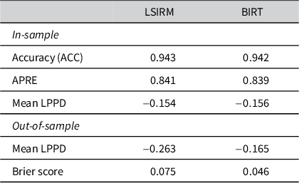
We evaluate predictive performance using classification accuracy (ACC), aggregate proportional reduction in error (APRE) and mean log posterior predictive density (LPPD). As shown in Table 2, Euclidean LSIRM and BIRT exhibit very similar in-sample predictive performance. LSIRM is slightly better on in-sample ACC, APRE and mean LPPD, but the differences are small. Out-of-sample performance is assessed using a 20% entry-wise holdout split. The held-out results also show that both models provide strong probabilistic predictions relative to an uninformative baseline. The Brier score measures the mean squared difference between predicted probabilities and actual binary outcomes, ranging from 0 to 1 with lower values indicating better probabilistic calibration; the uninformative baseline of always predicting $\hat {p} = 0.5$ yields a score of 0.25. Both models substantially improve upon this baseline, with Brier scores well below 0.25. These validation results indicate that Euclidean LSIRM remains predictively competitive with BIRT.

Table 2

In-sample and out-of-sample predictive performance for LSIRM and BIRT ( $K=2$ )

Table 2 Long description

The table consists of three columns. The first column lists the metrics, the second column provides values for L S I R M, and the third column provides values for B I R T.

In-sample results:

* Accuracy (A C C): L S I R M is 0.943, B I R T is 0.942.

* A P R E: L S I R M is 0.841, B I R T is 0.839.

* Mean L P P D: L S I R M is minus 0.154, B I R T is minus 0.156.

Out-of-sample results (based on a 20 percent entry-wise holdout):

* Mean L P P D: L S I R M is minus 0.263, B I R T is minus 0.165.

* Brier score: L S I R M is 0.075, B I R T is 0.046.

Note: Out-of-sample results are based on a 20% entry-wise holdout.

Beyond predictive performance, the Euclidean specification provides a useful representation of coalition structure through its joint metric embedding of legislators and bills. This has broader implications for ideal point estimation: legislatures where intra-party factionalism is consequential—such as those with multi-party systems, coalition governments or cross-cutting cleavages that do not map cleanly onto a single left–right axis—are precisely the settings where a non-metric distance formulation is most likely to obscure latent structure. In such contexts, recovering faction-level ideal points accurately is not only a methodological concern but a substantive one, as mismeasured positions can distort inferences about coalition formation, agenda influence and legislative bargaining.

Predictive gains from increasing dimensionality diminish beyond $K=2$ for Euclidean LSIRM (see Table B2 in the Supplementary Material). Because improvements beyond two dimensions are modest and the substantive coalition structure is already clearly recovered in two dimensions, we adopt $K=2$ for interpretation in the main analysis.

5.3 Bill embeddings as interpretive anchors

A key advantage of the bipartite network approach is that bill locations serve as interpretive anchors clarifying the substantive meaning of latent dimensions. Figure 6 displays the full legislator–bill embedding. Partisan bills cluster near their respective party centroids: Republican-supported bills (e.g., tax cuts and defense spending) locate in the far-right region near mainstream Republicans, while Democratic-supported bills (e.g., social programs and environmental regulation) cluster in the left region near mainstream Democrats. This validates that the first dimension captures the familiar liberal-conservative divide.

Figure 6

Two-dimensional legislator–bill ideal point estimates for the 118th U.S. House. Legislators are plotted by party and factional affiliation: Mainstream Democrats (blue squares), “Squad” Democrats (purple triangles), Mainstream Republicans (red circles) and Freedom Caucus Republicans (pink crosses). Bills are represented by gray markers.

Figure 6. Long description

The figure consists of two panels, a and b, both using a grid with X and Y axes from negative 4 to positive 4.

Panel a, titled Interaction Map, shows a dense distribution of gray dots representing bills forming a central horseshoe shape. Blue squares representing Mainstream Democrats are clustered in the upper-left quadrant between X negative 3 and negative 1, and Y 0 and 3. Purple triangles for Squad Democrats are located just below this group near Y negative 1. Red circles for Mainstream Republicans are clustered in the center-right area between X 0 and 2, and Y negative 1 and 1. Pink crosses for Freedom Caucus Republicans are scattered in the lower-right quadrant between X 2 and 4, and Y negative 2 and 0.

Panel b, titled Specific Bills, maintains the legislator clusters but highlights seven specific bills with black markers.

- H C O N R E S 2 1 Syria Withdrawal and H C O N R E S 3 0 Somalia Withdrawal are represented by a black square and circle in the lower-center at X negative 1, Y negative 2.

- H J R E S 7 9 Emergency is a black triangle at X negative 0.5, Y negative 2.

- H R 3 7 4 6 Debt Limit Deal is a black diamond at X negative 0.3, Y 0.5.

- H R 4 7 5 5 Privacy Tech Act is a square with a diagonal slash at X negative 0.6, Y 0.

- H R 5 4 0 3 C B D C is a circle with an X at X 1, Y 0.5.

More revealing are bills that deviate from party centroids. War powers resolutions H.Con.Res. 21 (Syria withdrawal), H.Con.Res. 30 (Somalia withdrawal) and H.J.Res. 79 (terminating national emergency) position in the lower-left quadrant between Squad and Freedom Caucus locations (coordinates approximately $x \approx -0.5$ , $y \approx -2$ ). These resolutions received support primarily from these two factions—progressive Democrats and libertarian Republicans—while being opposed by party establishments. Similarly, surveillance and privacy bills including H.R. 4755 (Privacy Enhancing Technology Research Act), H.R. 5403 (CBDC Anti-Surveillance State Act) locate far from the two extremist factions. These bill positions suggest the substantive meaning of the second dimension: it reflects an establishment-outsider cleavage where ideological extremes from both parties converge against centrists on issues of foreign military intervention and government surveillance—the “horseshoe” pattern where far-left and far-right align against the center (Duck-Mayr and Montgomery Reference Duck-Mayr and Montgomery2023).

The debt-limit deal H.R. 3746 positions near the center in LSIRM’s embedding ( $x \approx -0.4$ , $y \approx 0.5$ ), reflecting its passage through a Democratic-anchored coalition with substantial Republican support—a bipartisan compromise occupying ideological middle ground. In contrast, BIRT cannot provide this interpretation because bills are not embedded spatially. The discrimination parameter $\beta _j$ measures directional alignment but does not locate bills in the ideological space, precluding direct visualization of which bills define which dimensions. Without bill embeddings, conventional methods cannot directly show where such compromise legislation locates relative to partisan bills and extremist-coalition bills, obscuring the multi-dimensional coalition structure that characterizes contemporary congressional politics. Additional analyses in the Supplementary Material (Section 2.4) visualize bill locations together with within-faction Yea ratios, providing a finer-grained view of how factional support patterns align with Euclidean LSIRM’s spatial geometry.