1 Introduction
The convective circulation that results from heating and cooling at the same geopotential, or on a single horizontal boundary, such as the sea surface, has been studied for its relevance to large-scale ocean circulation (Stommel Reference Stommel1962; Rossby Reference Rossby1965; Hughes & Griffiths Reference Hughes and Griffiths2008; Saenz et al. Reference Saenz, Hogg, Hughes and Griffiths2012; Stewart, Hughes & Griffiths Reference Stewart, Hughes and Griffiths2012) and industrial processes (Chiu-Webster, Hinch & Lister Reference Chiu-Webster, Hinch and Lister2008). In contrast to convection driven by heating at the bottom and cooling at the top of a layer of fluid, where there is a net vertical heat flux and a substantial supply of gravitational potential energy (the tendency for the centre of gravity to be raised by the boundary buoyancy fluxes), horizontal convection in its statistically steady thermal equilibrium state is instead characterised by vanishing net heat flux (and buoyancy flux for a Boussinesq fluid) through the forcing boundary, and hence a very small supply of gravitational potential energy. The latter is due only to molecular diffusion of heat downwards in a small mean stable temperature gradient. This implies a strongly constrained rate of viscous dissipation (Paparella & Young Reference Paparella and Young2002; Scotti & White Reference Scotti and White2011; Gayen et al. Reference Gayen, Griffiths, Hughes and Saenz2013a ). These features make it a particularly interesting case of convection. However, studies of horizontal convection have been limited to the special class of boundary conditions varying in only one direction, and over the scale of the domain in which the fluid is free to flow. Here we refer to this class as the Rossby problem, originally motivated by a conceptual picture of the ocean circulation that might result from a global meridional gradient of sea surface thermal boundary conditions (Stommel Reference Stommel1962). Cases have been studied without background rotation (Rossby Reference Rossby1965, Reference Rossby1998; Paparella & Young Reference Paparella and Young2002; Mullarney, Griffiths & Hughes Reference Mullarney, Griffiths and Hughes2004; Scotti & White Reference Scotti and White2011; Sheard & King Reference Sheard and King2011; Gayen, Griffiths & Hughes Reference Gayen, Griffiths and Hughes2014) and with rotation in either axisymmetric (Hignett, Ibbetson & Killworth Reference Hignett, Ibbetson and Killworth1981) or rectangular geometry (Park & Whitehead Reference Park and Whitehead1999; Barkan, Winters & Llewellyn Smith Reference Barkan, Winters and Llewellyn Smith2013; Sheard, Hussama & Tsai Reference Sheard, Hussama and Tsai2016; Vreugdenhil, Gayen & Griffiths Reference Vreugdenhil, Gayen and Griffiths2016; Vreugdenhil, Griffiths & Gayen Reference Vreugdenhil, Griffiths and Gayen2017).
The Rossby problem shows that a coherent overturning circulation takes place through the width and depth of the convection domain, the structure of the flow closely tied to the distribution of heating at the forcing boundary. The overturning is highly asymmetric with a single, narrow vertical plume carrying destabilising buoyancy away from the forcing boundary. The plume is located either against the endwall of a closed box (if the boundary temperature distribution is monotonic; Rossby Reference Rossby1965; Mullarney et al.
Reference Mullarney, Griffiths and Hughes2004), or at the centre of the domain (for a sinusoidal boundary temperature with maximum at the centre; Paparella & Young Reference Paparella and Young2002). Aspect ratios have ranged from
 $H/L=1$
to
 $H/L=0.16$
, but scaling analyses for both viscous (Rossby Reference Rossby1965) and turbulent boundary layer (Gayen et al.
Reference Gayen, Griffiths and Hughes2014) regimes are governed by the boundary layer, so that the depth of the fluid does not influence heat transport, at least for depths not much greater than the length of the box. Most interest has focused on the thermal equilibrium state, in which the time average must have no net vertical heat transport through the forcing boundary or any geopotential level in the fluid. The flow is sensitive to departure from equilibrium and the consequent net buoyancy flux, and a challenge in simulation of the flow at large Rayleigh numbers is a long, computationally expensive equilibration time (Griffiths, Hughes & Gayen Reference Griffiths, Hughes and Gayen2013).
Another challenge in horizontal convection is that the turbulent boundary layer regime occurs only at very large values of the horizontal Rayleigh number
 $Ra=g\unicode[STIX]{x0394}\unicode[STIX]{x1D70C}L^{3}/\unicode[STIX]{x1D70C}_{0}\unicode[STIX]{x1D705}\unicode[STIX]{x1D708}$
(based on the horizontal length scale
 $L$
through which heat is transported, gravitational acceleration
 $g$
, applied density difference
 $\unicode[STIX]{x0394}\unicode[STIX]{x1D70C}$
, reference density
 $\unicode[STIX]{x1D70C}_{0}$
, fluid viscosity
 $\unicode[STIX]{x1D708}$
and thermal diffusivity
 $\unicode[STIX]{x1D705}$
). Simulations show that turbulence in the boundary layer governs the circulation, in a regime governed by buoyancy and inertia, at
 $Ra\gtrsim 10^{11}$
(and Prandtl numbers
 $Pr=\unicode[STIX]{x1D708}/\unicode[STIX]{x1D705}$
between 1 and 10; Gayen et al.
Reference Gayen, Griffiths and Hughes2014). Transitional, non-similar behaviour is found over the range
 $10^{9}<Ra<10^{12}$
. At the same time, vanishing net buoyancy flux through any level in the fluid implies a domain-integrated rate of viscous dissipation
 $\unicode[STIX]{x1D700}_{T}\leqslant ((\unicode[STIX]{x1D70C}_{0}\unicode[STIX]{x1D705}^{3}W/L^{3})a_{T}Ra\,Pr)/2$
, where
 $a_{T}$
is the horizontal area of the domain (Paparella & Young Reference Paparella and Young2002; Gayen et al.
Reference Gayen, Griffiths, Hughes and Saenz2013a
). A dominance of turbulent (over mean flow) dissipation implies an average Kolmogorov dissipation length scale
 $\unicode[STIX]{x1D702}_{K}=(\unicode[STIX]{x1D708}^{3}/\overline{\unicode[STIX]{x1D700}})^{1/4}$
(
 $\overline{\unicode[STIX]{x1D700}}$
the averaged dissipation rate per unit mass) that decreases with increasing Rayleigh number as
 $\unicode[STIX]{x1D702}_{K}/L\sim (H/L)^{1/4}Pr^{1/2}Ra^{-1/4}$
(Gayen et al.
Reference Gayen, Griffiths and Hughes2014). However, only the heated portion of the basal thermal boundary layer and the vertical endwall plume are turbulent at
 $Ra=O(10^{13})$
and shear production of turbulence surpasses convective production as the largest source of small-scale turbulent kinetic energy only at
 $Ra\gtrsim 10^{14}$
(Gayen et al.
Reference Gayen, Griffiths and Hughes2014). Simulations have not achieved conditions showing a well-developed inertial subrange in the interior of the flow, and therefore an asymptotic regime might not have been reached. The persistence of the
 $1/5$
power law scaling for heat transport in the Rossby problem through both laminar and turbulent regimes (with a larger pre-factor in the turbulent boundary layer regime), as well as the lack of turbulence production in the interior, can be attributed to stringent dynamical constraints imposed on the flow by the geometry: the largest scale of motion is locked to the distribution of heating and cooling, and is therefore two-dimensional and stationary in space.
An alternative arrangement of boundary conditions that allows the flow more degrees of freedom has temperature gradients in both horizontal directions and a length scale independent of the dimensions of the domain. These more general conditions were achieved in simulations (Griffiths & Gayen Reference Griffiths and Gayen2015) having a two-dimensional sinusoidal distribution of imposed boundary temperatures. The arrangement is conceptually equivalent to a large number of Rossby horizontal convection domains (albeit changed to roughly circular regions) placed end to end in both horizontal directions. The cold regions produce a dense boundary layer on the base that converges towards each warm patch, where the fluid is heated and potentially ascends in an array of buoyant, three-dimensional plumes. Simulations of a square box of width
 $W$
equal to three of four forcing wavelengths
 $L$
in each direction and
 $Ra=10^{12}$
(where for consistency with the Rossby problem
 $Ra$
was based on the horizontal scale
 $L$
of the forcing rather then the box width) showed that the flow again evolves to a thermal equilibrium state having vanishing net heat and buoyancy fluxes through the boundary. For shallow water depth
 $H$
(a small aspect ratio
 $H/L=0.5$
) the mean flow consisted of an array of approximately axisymmetric plumes, a plume ascending from each warm patch of the boundary. The plumes were turbulent.
A very different behaviour was found for deep water (a large aspect ratio,
 $H/L=5$
) with the same sinusoidal temperature conditions and the wider domain (
 $W=4L$
). In that case individual plumes from the heated patches were only intermittently identifiable. Instead, large scales of circulation emerged, the most energetic motions having the dimensions of the computational domain. These simulations also showed a
 $-5/3$
Kolmogorov energy spectrum everywhere in the interior and a log-law in the boundary layer, and production of small scales predominantly by shear rather than by the turbulent buoyancy flux. The large-scale circulation was not a single circulation cell having a single scale or primarily vertical shear; it was equant (as were the box aspect ratios used:
 $H/W=5/4$
and square planform), unsteady, showed low-frequency reversals, gave shear production of small scales from all velocity components, and was made up of a range of small wavenumbers that are an integral part of the turbulence spectrum. These are characteristics in common with the large scales of circulation found in Rayleigh–Bénard convection at Rayleigh numbers greater than
 $10^{9}$
(Gayen, Hughes & Griffiths Reference Gayen, Hughes and Griffiths2013b
).
Insights into the nature of horizontal convection are also found in the mechanical energy conversions. The absence of a net vertical buoyancy flux leaves only a very small supply of gravitational potential energy (the tendency to raise the centre of gravity of the fluid, in this case due to molecular diffusion of heat downwards through the depth of the domain between the horizontally averaged temperatures at the top and bottom of the domain). Viscous dissipation is an equally small energy sink (Paparella & Young Reference Paparella and Young2002). However, the supply of available potential energy (APE), which is required to drive motion (Winters et al.
Reference Winters, Lombard, Riley and D’Asaro1995; Hughes, Hogg & Griffiths Reference Hughes, Hogg and Griffiths2009), is orders of magnitude greater than the viscous dissipation rate in horizontal convection (Scotti & White Reference Scotti and White2011; Gayen et al.
Reference Gayen, Griffiths, Hughes and Saenz2013a
, Reference Gayen, Griffiths and Hughes2014). This is because APE supply is the sum of the potential energy production and a very much larger rate of conversion (with no change in potential energy) of background potential energy into APE (where the background describes a reference state of gravitation equilibrium, hence no motion). Both conversions are due to the surface buoyancy forcing. Thus, while the absence of a net vertical buoyancy flux imposes strong constraints on horizontal convection, these by no means limit the flow to be laminar: transition to the turbulent boundary layer regime described above begins with the first instabilities occuring at
 $Ra\approx 10^{9}$
and an asymptotic regime is reached at
 $Ra\approx 10^{12}$
(Gayen et al.
Reference Gayen, Griffiths and Hughes2014). The statistically steady state must have the conversion from background to available potential energy in balance with the return conversion (from available to background potential energy), and this is achieved by irreversible mixing of density down the local density gradients in the gravitational field. Mixing is a sink of APE and, while the mixing is found to be strongly confined to the thermal boundary layer, the domain-integrated rate of mixing in horizontal convection is very large compared to the total rate of viscous dissipation. It follows that the ratio of the integrated mixing rate to the sum of the two mechanical energy sinks (termed the ‘mixing efficiency’,
 $\unicode[STIX]{x1D702}$
) is close to 1. In the Rossby problem the rate of production of APE relative to viscous dissipation is of the order of
 $10^{2}$
and mixing efficiency
 $\unicode[STIX]{x1D702}\approx 95\,\%$
at
 $Ra=10^{12}$
(Gayen et al.
Reference Gayen, Griffiths, Hughes and Saenz2013a
, Reference Gayen, Griffiths and Hughes2014). For the two-dimensional array forcing, the production of APE relative to dissipation at this value of
 $Ra$
is approximately
 $10^{3}$
and the mixing efficiency is
 $\unicode[STIX]{x1D702}\approx 99\,\%$
, and yet shear production of turbulence kinetic energy and its dissipation occur throughout the domain (Griffiths & Gayen Reference Griffiths and Gayen2015). The different rates of APE production and mixing, and the different mixing efficiencies in horizontal convection driven by these two forcing distributions stem almost entirely from different density gradients at the forcing boundary. In this paper we address the dynamics of the array convection that lead to greater APE production.
In contrast, most other convection problems involve a more substantial supply of potential energy due to a net vertical buoyancy flux. For example, in Rayleigh–Bénard convection the supply of available potential energy that maintains the flow arises in equal measure from the production of potential energy (i.e. raising the centre of gravity of the fluid) by the net vertical buoyancy flux, and from the conversion of background potential energy to APE (with no change in total potential energy) by boundary buoyancy fluxes (Hughes, Gayen & Griffiths Reference Hughes, Gayen and Griffiths2013; Gayen et al.
Reference Gayen, Hughes and Griffiths2013b
). The statistically steady state must have a balance between the conversion from background to available PE, in one direction, and the rate of removal of APE by irreversible mixing in the other direction, as in horizontal convection. However, the production of potential energy by the net buoyancy flux in Rayleigh–Bénard convection is nearly equal to the conversion of APE to kinetic energy (and the effects of diffusion down the mean temperature gradient are negligible at large Rayleigh numbers). Since the total viscous dissipation of kinetic energy in the domain is given by the net kinetic energy generation, the mixing efficiency in this case approaches
 $\unicode[STIX]{x1D702}\approx 1/2$
at large Rayleigh numbers. Despite these major differences, Rayleigh–Bénard convection shares with horizontal convection (when forced by a two-dimensional array of boundary heating and cooling) the emergence of large-scale circulation at one end of the turbulence kinetic energy spectrum, a dominance of these largest scales for buoyancy transport, and turbulence production by shear instability throughout the bulk of the fluid.
It remains to be shown whether the simulated transition to large-scale circulation in domains much larger than the forcing length scale can be realised in the laboratory, what conditions determine the regime transition, and how the flow and heat throughput scale with Rayleigh number. This arrangement helps to place the traditional Rossby problem, and the constraints it imposes on the convection, into a broader context. Here we report laboratory experiments with a forcing arrangement analogous to the thermal forcing introduced in Griffiths & Gayen (Reference Griffiths and Gayen2015), for a box width
 $W=4L$
, but using instead compositional convection (having Schmidt number of 760) in order to achieve a similarly large value of the horizontal Rayleigh number. The laboratory flow demonstrates equilibration to a state of zero net buoyancy flux, and either the persistence of multiple turbulent plumes with dynamics similar to the Rossby problem, or the development of turbulent larger scale overturning, depending on aspect ratio. We then use Direct Numerical Simulations for the thermal convection case (with
 $W=4L$
and a Prandtl number of 1) in order to determine the Rayleigh number scaling of mechanical energy conversions and heat flux in each regime for two fluid depths. Predictions for adjustment to the statistically steady state of compositional convection and the experimental methods are outlined in § 2, the laboratory results are reported in § 3, the simulations of thermal convection are described in § 4, scaling analysis is discussed in § 5 and concluding remarks are given in § 6.
2 Laboratory experiments
It is not practical to achieve the large Rayleigh number values of interest using heating and cooling in the laboratory, given that forcing is to be applied on a length scale much smaller than the width and depth of a laboratory tank. We therefore use compositional convection driven by concentration differences of aqueous NaCl solution. The aim is not to mimic thermal convection, but rather to investigate the behaviour of horizontal convection under a spatially periodic forcing at
 $Ra>10^{11}$
. The use of compositional convection, which necessarily has boundary conditions somewhat different from those in the thermal convection simulations, also contributes to knowledge of the robustness of the results. Previous horizontal convection experiments have used salinity- and freshwater inputs to reconstruct the Rossby problem (Pierce & Rhines Reference Pierce and Rhines1996) and to add artificial turbulent mixing to the problem (Whitehead & Wang Reference Whitehead and Wang2008; Stewart et al.
Reference Stewart, Hughes and Griffiths2012).
2.1 Apparatus
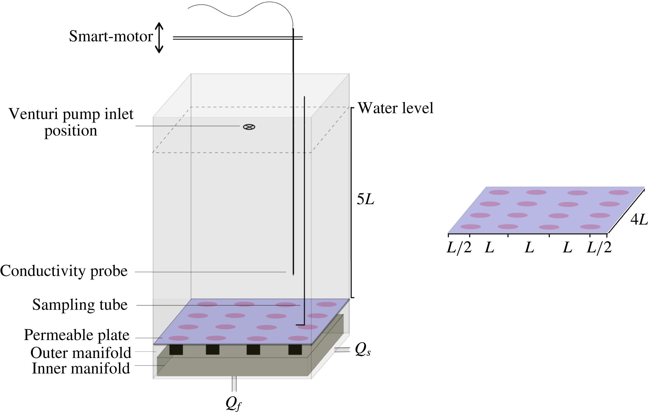
The experiments were carried out in a deep, square box of internal width
 $W=0.3$
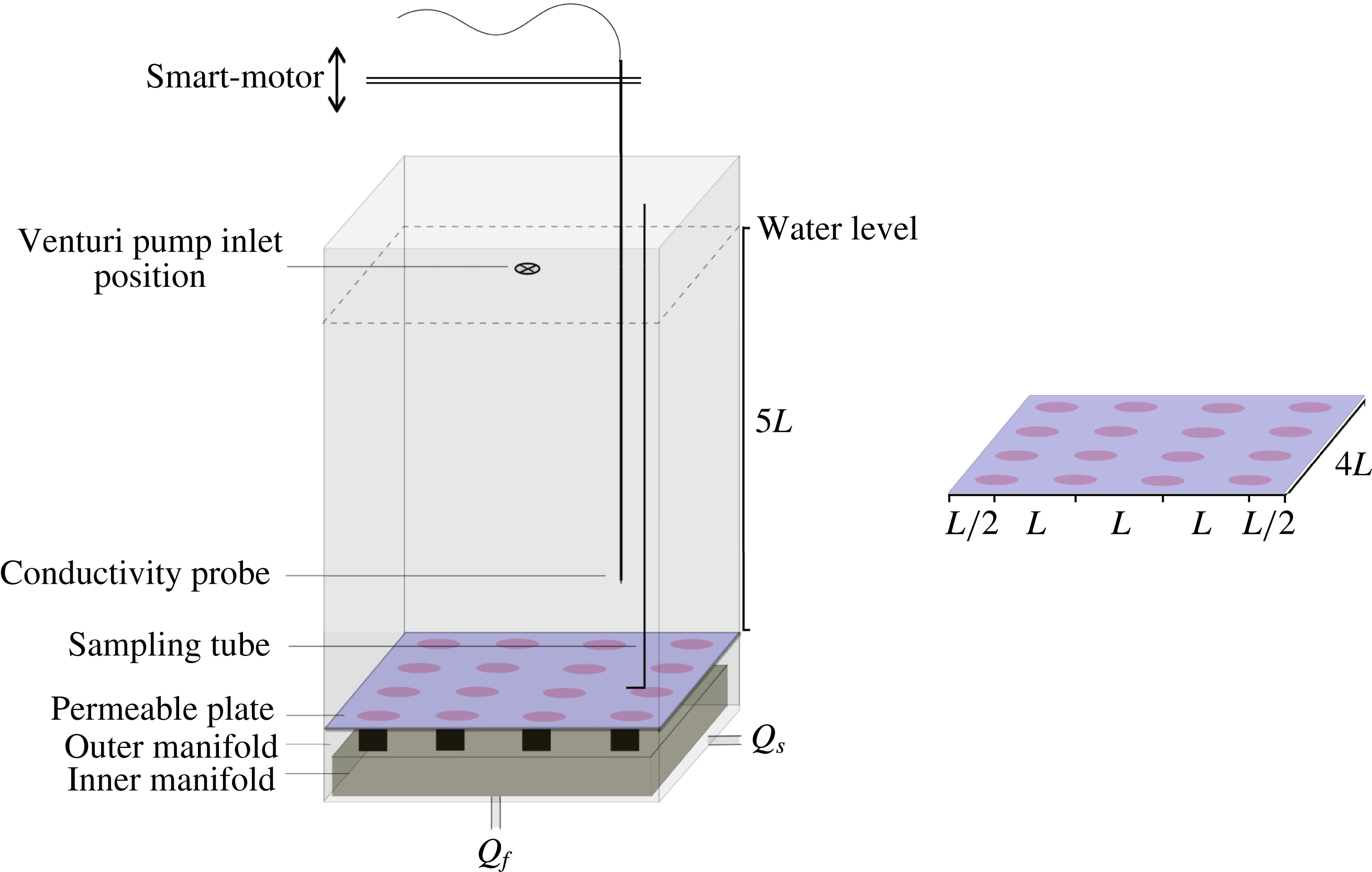
m and height 0.55 m, with a permeable sintered brass plate as the horizontal bottom boundary for the convection domain (figure 1). Below the permeable plate was a chamber filled with saline solution that was in contact with the permeable plate and slightly pressurised from an external supply reservoir. This chamber also housed an inner manifold which supplied relatively fresh water to small circular areas of the permeable plate through a square array of cylinders, each 25 mm diameter, separating the freshwater from the saline water. In most experiments the inner manifold supplied 16 circular regions, centred a distance
 $L=75$
mm apart in a
 $4\times 4$
array, which in turn was symmetrically arranged within the width of the box. A few experiments were carried out with a similarly symmetric
 $3\times 3$
array of fresh inputs. Peristaltic pumps coupled with flow integrators (to smooth the pump outputs) were used to supply constant volume fluxes (as measured by flowmeters) of de-aerated, filtered saline solution and freshwater to the manifolds from external reservoirs. Both reservoirs were kept well mixed, ensuring constant input salinities throughout a run.
Schematic of the laboratory apparatus showing the forcing arrangement, with regions of dense saline (blue) and buoyant freshwater (red) input at the permeable base, and vertical cylinders supplying freshwater (at flux
 $Q_{f}$
) from the inner manifold to the permeable plate (black). The sketch shows the water depth for the deep case and the forcing array for the wavelength
 $L=75$
mm,
 $W/L=4$
. The separate planform of the density distribution at the base shows the symmetric arrangement of forcing with respect to the sidewalls.
The approach is the same as used to study ‘pure’ buoyant plumes (Baines & Turner Reference Baines and Turner1969), where a finite but small and dynamically insignificant volume flux is required to deliver the buoyancy. For the present experiments the effect of the small volume input on the bottom boundary layer is evaluated in § 2.3. In order to limit the final water depth
 $H$
and allow the convection to approach a true statistically steady state, water was also removed from the top by placing the inlet of a Venturi pump on the centreline of the tank at the desired final water depth. This sink withdrew water and salt, but represented zero buoyancy flux (
 $g\unicode[STIX]{x1D70C}^{\prime }(Q_{s}+Q_{f})$
), as the density of solution withdrawn is identical to that of the bulk of the box (
 $\unicode[STIX]{x1D70C}^{\prime }=0$
). The location of the sink at the top also ensures that the withdrawal has negligible influence on the density of the bulk of the box and the individual saline and freshwater buoyancy fluxes at the base. The small volume throughput and associated small mean vertical velocity
 $\overline{w}\approx (Q_{f}+Q_{s})/W^{2}$
(which will be seen to be around 20 times smaller than the average convection velocities in the interior) also ensure that the sink has no significant influence on the convective velocity field. Adequate quasi-steady states were reached before the water surface reached the sink, as water depth increased very slowly. However, the increasing depth did not suit long measurement periods required to obtain time-averaged flow statistics. Hence the measurements reported here are from the final, true equilibrium states having constant
 $H$
. Experiments were carried out with
 $H=150$
mm (
 $H/L=2$
) and
 $H=375$
mm (
 $H/L=5$
).
Conductivity measurements were made using a PME MicroScale Conductivity and Temperature probe (Model 125) attached to a traversing mechanism, in turn driven by a Smart Motor and controlled by a computer program. Vertical profiles of conductivity were taken at regular intervals, excepting when high-resolution time records were required, in which case the probe was placed at a fixed location for the desired duration of the record. The location of the probe was varied in one horizontal (
 $x$
) direction in order to obtain profiles above both saline and freshwater input areas. Direct density measurements of samples, withdrawn from various heights through a tube at
 $(x,y)=(75~\text{mm},112.5~\text{mm})$
, were made using an Anton Paar digital densimeter (Model DMA5000; precision of
 $\pm 1\times 10^{-6}~\text{g}~\text{cm}^{-3}$
).
Two-component velocity fields (
 $u,w$
) were obtained by particle tracking velocimetry (PTV). For this the flow was seeded with 125–
 $250~\unicode[STIX]{x03BC}\text{m}$
diameter particles of Pliolite resin and illuminated from the side in a vertical plane by a light sheet from a 250 W white light projector beam passing through a 5 mm slit at the wall of the box. Input salinities (particularly of the fresher input) and flow rates were chosen such that the bulk density in the convection domain in the final equilibrium state (as predicted theoretically in § 2.3) was approximately
 $1021~\text{kg}~\text{m}^{-3}$
, matching the density of the Pliolite. Particle motion was recorded, at 25 f.p.s., by a high-definition video camera mounted 4 m from the box, the movie later decomposed into images, particles identified and tracked, and their velocities estimated using the Streams package (Nokes Reference Nokes2014). The particle-centred velocities were then interpolated onto a regular grid at each time step, yielding a time series of two components of the Eulerian velocity field on the measurement plane. In separate runs dedicated to qualitative flow visualisation the same light sheet was used to illuminate fluorescein dye, which was introduced to the freshwater input in trace concentrations.
2.2 Experimental parameters
The governing parameters for these isothermal experiments may be written as the solutal Rayleigh number
 $Ra_{s}$
(based on the horizontal forcing scale
 $L$
and solute diffusivity
 $\unicode[STIX]{x1D705}_{s}$
), the Schmidt number
 $Sc$
, the dimensionless depth and width of the convection domain, a Peclet number
 $Pe$
based on input flow rate, and the ratio
 $R_{Q}$
of destabilising to stabilising volume fluxes:
 $$\begin{eqnarray}Ra_{s}\equiv g\unicode[STIX]{x0394}\unicode[STIX]{x1D70C}L^{3}/\unicode[STIX]{x1D70C}_{0}\unicode[STIX]{x1D705}_{s}\unicode[STIX]{x1D708},\quad Sc\equiv \frac{\unicode[STIX]{x1D708}}{\unicode[STIX]{x1D705}_{s}},\quad A\equiv H/L,\quad n\equiv W/L,\end{eqnarray}$$
 $$\begin{eqnarray}Pe\equiv Q_{f}/\unicode[STIX]{x1D705}_{s}L,\quad R_{Q}\equiv Q_{f}/Q_{s},\end{eqnarray}$$
where
 $\unicode[STIX]{x0394}\unicode[STIX]{x1D70C}$
is the applied density difference between the two input solutions of salinity
 $S_{f}$
and
 $S_{s}$
, and
 $Q_{f}$
,
 $Q_{s}$
are the corresponding area-integrated imposed volume input rates of the relatively fresh and saline inputs, respectively. The width
 $W$
was designed to be an integer multiple
 $n$
of the forcing wavelength
 $L$
. Note that the Rayleigh number in the Rossby problem is often based on only one half of the forcing wavelength (heating near one end and cooling near the other end over a box length
 $L$
), whereas
 $Ra$
is here based on the full wavelength of the forcing and is therefore eight times larger than the more common horizontal Rayleigh number. Given that both the input salinities and the volume fluxes are also imposed, a flux Rayleigh number can also be defined as
 $Ra_{F}=gQ_{f}\unicode[STIX]{x0394}\unicode[STIX]{x1D70C}L^{2}/\unicode[STIX]{x1D70C}_{o}\unicode[STIX]{x1D708}\unicode[STIX]{x1D705}_{s}^{2}=Ra_{s}Pe$
.
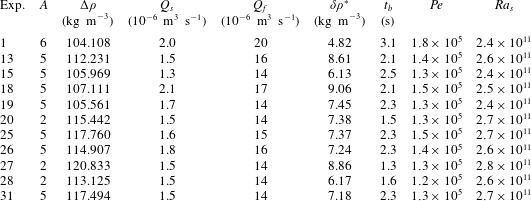
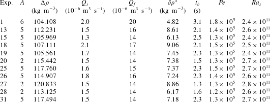
The conditions for a series of experiments are summarised in table 1. In this series each experiment commenced with 50 mm of solution above the permeable base at a density greater than the expected final density in the bulk of the domain. The water freshened as the box very slowly filled. Before quasi-equilibrium density was reached the smaller of the input densities drove bottom-to-surface convection. The average salinity of the bulk of the domain eventually approached a constant or equilibrium value, and convection was then maintained by the differential buoyancy inputs. Once the water surface reached the level of the withdrawal sink, the experiment continued with a constant water depth. The water depth could later be increased by raising the sink to a higher level and allowing a further period of equilibration.
Summary of experimental conditions in runs with
 $n=4$
: imposed density difference
 $\unicode[STIX]{x0394}\unicode[STIX]{x1D70C}=\unicode[STIX]{x1D70C}_{s}-\unicode[STIX]{x1D70C}_{f}$
(
 $\pm 0.005$
), volume flow rates
 $Q_{s}$
(
 $\pm 0.3\times 10^{-6}$
) and
 $Q_{f}$
(
 $\pm 1\times 10^{-6}$
) of saline and fresher inputs, measured density difference
 $\unicode[STIX]{x1D6FF}\unicode[STIX]{x1D70C}^{\ast }=\bar{\unicode[STIX]{x1D70C}}^{\ast }-\unicode[STIX]{x1D70C}_{f}$
(
 $\pm 0.05$
) between the bulk and the fresher input at equilibrium, buoyancy time scale
 $t_{b}=[(H/g)(\unicode[STIX]{x1D70C}_{f}/\unicode[STIX]{x1D6FF}\unicode[STIX]{x1D70C}^{\ast })]^{1/2}$
, Peclet number and Rayleigh number. All runs had
 $\unicode[STIX]{x1D705}_{s}\approx 1.5\times 10^{-9}~\text{m}^{2}~\text{s}^{-1}$
,
 $Sc\approx 760$
and measurements were generally taken for water depths of
 $H\approx 2L$
and
 $H\approx 5L$
. Uncertainty in
 $\unicode[STIX]{x1D6FF}\unicode[STIX]{x1D70C}^{\ast }$
is given by one standard deviation, after steady state was reached.
2.3 Theoretical equilibrium states
For constant volume flow rates of two solutions through a permeable base, into a box initially containing a small volume
 $V_{0}$
of density
 $\unicode[STIX]{x1D70C}_{0}$
, the total mass of solution in the box at time
 $t$
is
 $M=\unicode[STIX]{x1D70C}_{s}Q_{s}t+\unicode[STIX]{x1D70C}_{f}Q_{f}t+\unicode[STIX]{x1D70C}_{0}V_{0}$
. For a density
 $\unicode[STIX]{x1D70C}=\unicode[STIX]{x1D70C}_{0}\,f(S)$
(where
 $f$
is an arbitrary function,
 $S$
is salinity and
 $\unicode[STIX]{x1D70C}_{0}$
is a reference density) the mass of salt divided by the total mass of solution gives a bulk salinity
 $\bar{S}$
:
 $$\begin{eqnarray}\bar{S}(t)=\frac{\unicode[STIX]{x1D70C}_{s}S_{s}Q_{s}t+\unicode[STIX]{x1D70C}_{0}S_{0}V_{0}}{(\unicode[STIX]{x1D70C}_{s}Q_{s}+\unicode[STIX]{x1D70C}_{f}Q_{f})t+\unicode[STIX]{x1D70C}_{0}V_{0}}.\end{eqnarray}$$
Taking
 $\unicode[STIX]{x1D70C}_{f}\leqslant \unicode[STIX]{x1D70C}_{0}<\unicode[STIX]{x1D70C}_{s}$
, the solution becomes increasingly saline and approaches the large-time limit (denoted throughout by superscript ∗)
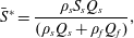 $$\begin{eqnarray}\bar{S}^{\ast }=\frac{\unicode[STIX]{x1D70C}_{s}S_{s}Q_{s}}{(\unicode[STIX]{x1D70C}_{s}Q_{s}+\unicode[STIX]{x1D70C}_{f}Q_{f})},\end{eqnarray}$$
at times
 $t\gg t_{eq}=\unicode[STIX]{x1D70C}_{0}S_{0}V_{0}/\unicode[STIX]{x1D70C}_{s}S_{s}Q_{s}$
(assuming
 $Q_{s}<Q_{f}$
). In this limit the added mass of salt becomes large compared to the initial mass of salt. Thus the average salinity is constant at large times. If
 $Q_{s}\ll Q_{f}$
, the equilibrium salinity (2.4) is
 $\bar{S}^{\ast }\approx \unicode[STIX]{x1D70C}_{s}S_{s}Q_{s}/\unicode[STIX]{x1D70C}_{f}Q_{f}$
and is much closer to the salinity of the fresher input than to that of the saline input. The salinity (2.4) is identical to that expected for a steady state in which the same saline and freshwater are injected continuously into any well-mixed box, with or without a matching volume flux from a sink. Hence the addition of the sink that withdraws the mixture in the convection experiments does not influence the bulk salinity and this, in turn, implies it has no influence on the input buoyancy fluxes.
The buoyancy fluxes into the box are determined by the bulk salinity predicted above. Once the bulk has reached the large-time equilibrium salinity the individual buoyancy fluxes carried by the fresher and more saline inputs become, respectively,
 $$\begin{eqnarray}B_{f}=g(\bar{\unicode[STIX]{x1D70C}}^{\ast }-\unicode[STIX]{x1D70C}_{f})Q_{f}/\unicode[STIX]{x1D70C}_{0},\quad B_{s}=g(\bar{\unicode[STIX]{x1D70C}}^{\ast }-\unicode[STIX]{x1D70C}_{s})Q_{s}/\unicode[STIX]{x1D70C}_{0},\end{eqnarray}$$
where
 $\bar{\unicode[STIX]{x1D70C}}^{\ast }=\unicode[STIX]{x1D70C}_{0}\,f(\bar{S}^{\ast })$
is the equilibrium density. Defining
 $\unicode[STIX]{x1D6FF}\unicode[STIX]{x1D70C}^{\ast }=\bar{\unicode[STIX]{x1D70C}}^{\ast }-\unicode[STIX]{x1D70C}_{f}$
, and recalling
 $\unicode[STIX]{x1D70C}_{s}-\unicode[STIX]{x1D70C}_{f}=\unicode[STIX]{x0394}\unicode[STIX]{x1D70C}$
, the destabilising buoyancy input is
 $B_{f}=g(\unicode[STIX]{x1D6FF}\unicode[STIX]{x1D70C}^{\ast }/\unicode[STIX]{x1D70C}_{0})Q_{f}$
and the stabilising input is
 $B_{s}=g[(\unicode[STIX]{x1D6FF}\unicode[STIX]{x1D70C}^{\ast }-\unicode[STIX]{x0394}\unicode[STIX]{x1D70C})/\unicode[STIX]{x1D70C}_{0}]Q_{s}$
. The net boundary buoyancy input is
 $$\begin{eqnarray}B=B_{f}+B_{s}=(g/\unicode[STIX]{x1D70C}_{0})[\bar{\unicode[STIX]{x1D70C}}^{\ast }(Q_{f}+Q_{s})-(\unicode[STIX]{x1D70C}_{s}Q_{s}+\unicode[STIX]{x1D70C}_{f}Q_{f})].\end{eqnarray}$$
In the case of a linear equation of state
 $\bar{\unicode[STIX]{x1D70C}}^{\ast }=(\unicode[STIX]{x1D70C}_{s}Q_{s}+\unicode[STIX]{x1D70C}_{0}Q_{f})/(Q_{f}+Q_{s})$
,
 $\unicode[STIX]{x1D6FF}\unicode[STIX]{x1D70C}^{\ast }/\unicode[STIX]{x0394}\unicode[STIX]{x1D70C}=Q_{s}/(Q_{s}+Q_{f})$
and (from (2.6)) the net boundary buoyancy input
 $B$
in the equilibrium state vanishes. This is a good approximation across the whole range of source salinities used in the present experiments. The accuracy of the approximation is further assured in the bulk of the fluid, where property differences are small compared to those in the dense boundary layer on the base. Thus the net buoyancy flux through any level vanishes at large times
 $t\gg t_{eq}$
. During the evolution to the steady state the assumption that the bulk remains well mixed requires the equilibration to be slow compared to the convective overturn, thus
 $t_{eq}\gg t_{b}$
, where
 $t_{b}=[(H/g)(\unicode[STIX]{x1D70C}_{f}/\unicode[STIX]{x1D6FF}\unicode[STIX]{x1D70C}^{\ast })]^{1/2}$
is the buoyancy time scale. In the steady state having zero net buoyancy flux through any level, the convective overturn need only be rapid compared to the very slow mean vertical velocity imposed by the finite volume throughput, a condition easily satisfied in the experiments.
For the linear equation of state the individual buoyancy inputs become
 $$\begin{eqnarray}B_{f}=-B_{s}=g(\unicode[STIX]{x0394}\unicode[STIX]{x1D70C}/\unicode[STIX]{x1D70C}_{0})[Q_{s}Q_{f}/(Q_{f}+Q_{s})]\end{eqnarray}$$
and in the limit
 $Q_{f}\gg Q_{s}$
 $$\begin{eqnarray}B_{f}\approx g(\unicode[STIX]{x0394}\unicode[STIX]{x1D70C}/\unicode[STIX]{x1D70C}_{0})Q_{s}.\end{eqnarray}$$
In this limit the corresponding Nusselt number describing the buoyancy throughput relative to a purely diffusive lateral transport can be written as
 $$\begin{eqnarray}Nu=Ra_{F}^{\ast }/Ra_{s}=Pe/R_{Q}=Q_{s}L/\unicode[STIX]{x1D705},\end{eqnarray}$$
where
 $Ra_{F}^{\ast }$
is a flux Rayleigh number
 $$\begin{eqnarray}Ra_{F}^{\ast }=B_{f}L^{2}/\unicode[STIX]{x1D708}\unicode[STIX]{x1D705}_{s}^{2}=Ra_{s}Pe/R_{Q}\end{eqnarray}$$
based on the actual destabilising buoyancy input (rather than on the external variables in (2.1)).
The bottom boundary conditions in the experiments are of mixed kind, as both densities and fluxes are imposed at the permeable base. Furthermore, both diffusive and advective fluxes may be significant at the boundary. The role of imposed fluxes is minimised if the salinity of the saline input is very large, so that the flow is characterised by
 $\unicode[STIX]{x1D6FF}\unicode[STIX]{x1D70C}^{\ast }\ll \unicode[STIX]{x0394}\unicode[STIX]{x1D70C}$
, which leaves the saline input as an imposed flux condition
 $Q_{s}S_{s}$
. The effect of a non-zero vertical velocity through the permeable boundary can be assessed by recalling that scaling analysis of the Rossby problem (Rossby Reference Rossby1965, Reference Rossby1998) treats the boundary layer as governed by a balance of vertical advection and diffusion, so that (in the absence of a volume flux through the boundary) the flow has a vertical (downward) velocity
 $w_{bl}\sim \unicode[STIX]{x1D705}/\unicode[STIX]{x1D6FF}$
, where
 $\unicode[STIX]{x1D6FF}$
is the boundary layer of thickness. An approximation for the boundary layer thickness can then be found by assuming simple horizontal momentum balances in the boundary layer, either viscous buoyancy (Rossby Reference Rossby1965, Reference Rossby1998) or inertial buoyancy (Gayen et al.
Reference Gayen, Griffiths and Hughes2014, equation (5.3)). The viscous balance, expected to give the smallest
 $w_{bl}$
and valid only at small values of
 $Ra$
, taken together within continuity, leads to
 $\unicode[STIX]{x1D6FF}/L\sim Ra^{-1/5}$
, which gives
 $\unicode[STIX]{x1D6FF}\sim 1$
mm for the Rayleigh numbers in the present compositional convection. The normal velocity imposed at the permeable base in the stabilised areas,
 $\overline{w_{s}}\approx Q_{s}/W^{2}$
, reduces the role of diffusion in governing boundary layer thickness and is likely to thicken the boundary layer over that given by the Rossby scaling when
 $\overline{w_{s}}>w_{bl}$
, or
 $Pe>n^{2}Ra^{1/5}$
. For the experiments this equates to
 $Pe>10^{6}$
and implies that for the experimental conditions (table 1) the boundary layer is unlikely to be influenced by the volume input. However, the precise nature of the boundary conditions is not important to our conclusions.
3 Experimental results
3.1 Equilibration of density
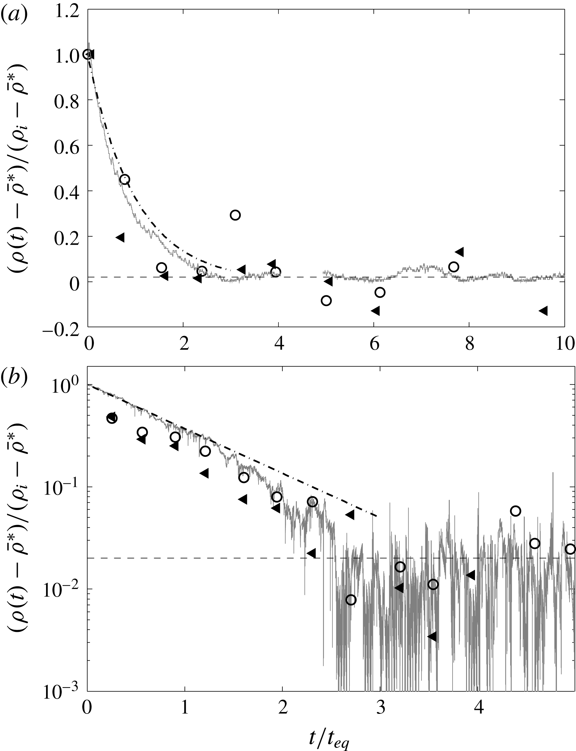
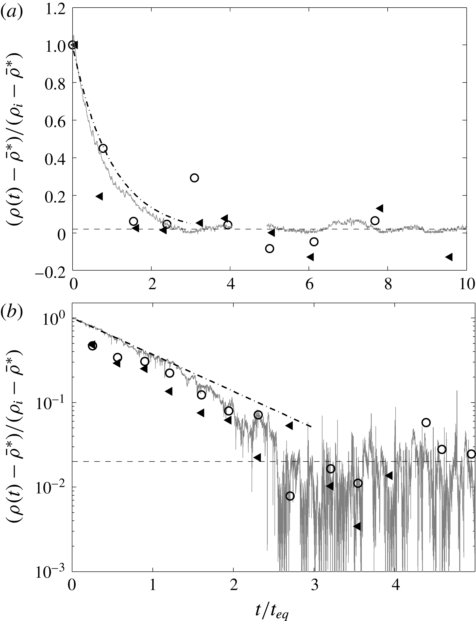
Experiments began with a small volume of saline solution in the box and a net destabilising buoyancy flux through the base, causing the density in the bulk of the water to decrease with time. The water depth increased slowly until the surface reached the sink. The system reached an equilibrium state in which the density at any location showed no further secular trend, fluctuating about a mean value (figure 2). The adjustment was approximately exponential with a time scale close to the predicted
 $t_{eq}$
, and equilibrium was reached by
 $t\approx 3t_{eq}$
. In the equilibrium state (for
 $Q_{s}\sim 0.1Q_{f}$
) the density difference between the bulk and the fresher input,
 $\unicode[STIX]{x1D6FF}^{\ast }=\bar{\unicode[STIX]{x1D70C}}^{\ast }-\unicode[STIX]{x1D70C}_{f}$
, was 5 %–9 % of the applied density difference
 $\unicode[STIX]{x0394}\unicode[STIX]{x1D70C}$
(table 1), and slightly fresher than predicted by (2.4).
Evolution of densities relative to the large time mean in the interior: (a) shallow-water case (exp. 20), plotted with a linear ordinate; and (b) deep-water case (exp. 31) plotted on a logarithmic ordinate. Symbols show density from samples (taken at
 $z/L=1$
and
 $z/L=3.7$
in the deep case and
 $z/L=0.5$
and
 $z/L=1.5$
in the shallow case, circles and triangles) and the continuous grey line shows in situ conductivity (at
 $z=3.7L$
in the deep case and
 $z/L=1.5$
in the shallow case). Densities are normalised by the overall change from initial to final local interior density and plotted as a function of elapsed time
 $t$
from the beginning of the experiment. Time is normalised by the equilibration time scale
 $t_{eq}=(\unicode[STIX]{x1D70C}_{0}S_{0}V_{0})t/(\unicode[STIX]{x1D70C}_{s}S_{s}Q_{s})$
. Fluctuations of
 $\unicode[STIX]{x1D70C}(t)$
about the mean equilibrium value
 $\bar{\unicode[STIX]{x1D70C}}^{\ast }$
are both positive and negative and therefore in (b) the absolute value is plotted. An empirical fit of
 $\unicode[STIX]{x1D6FD}\text{e}^{-t/t_{eq}}$
and the 98 % adjustment level are shown as dot-dashed and dashed lines respectively.
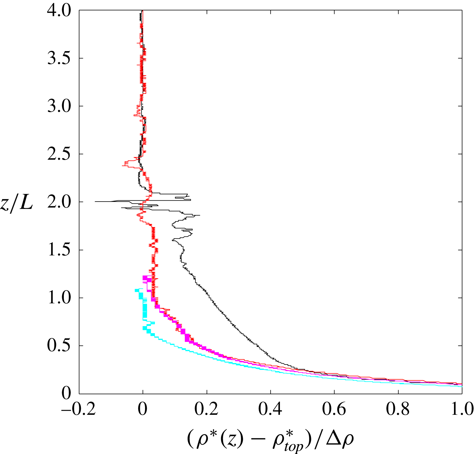
Vertical profiles of density from two deep-water cases (
 $A=5$
; exps 25, 26; red and black) and two shallow-water experiments (
 $A=2$
; exps 27, 28, cyan and magenta) in the equilibrium states. Density
 $\unicode[STIX]{x1D70C}^{\ast }$
is shown relative to the density
 $\unicode[STIX]{x1D70C}_{top}^{\ast }$
at the top of the profile and normalised by the applied density difference
 $\unicode[STIX]{x0394}\unicode[STIX]{x1D70C}$
. Profiles cover approximately
 $2/3$
of the water column to 5 mm from the base.
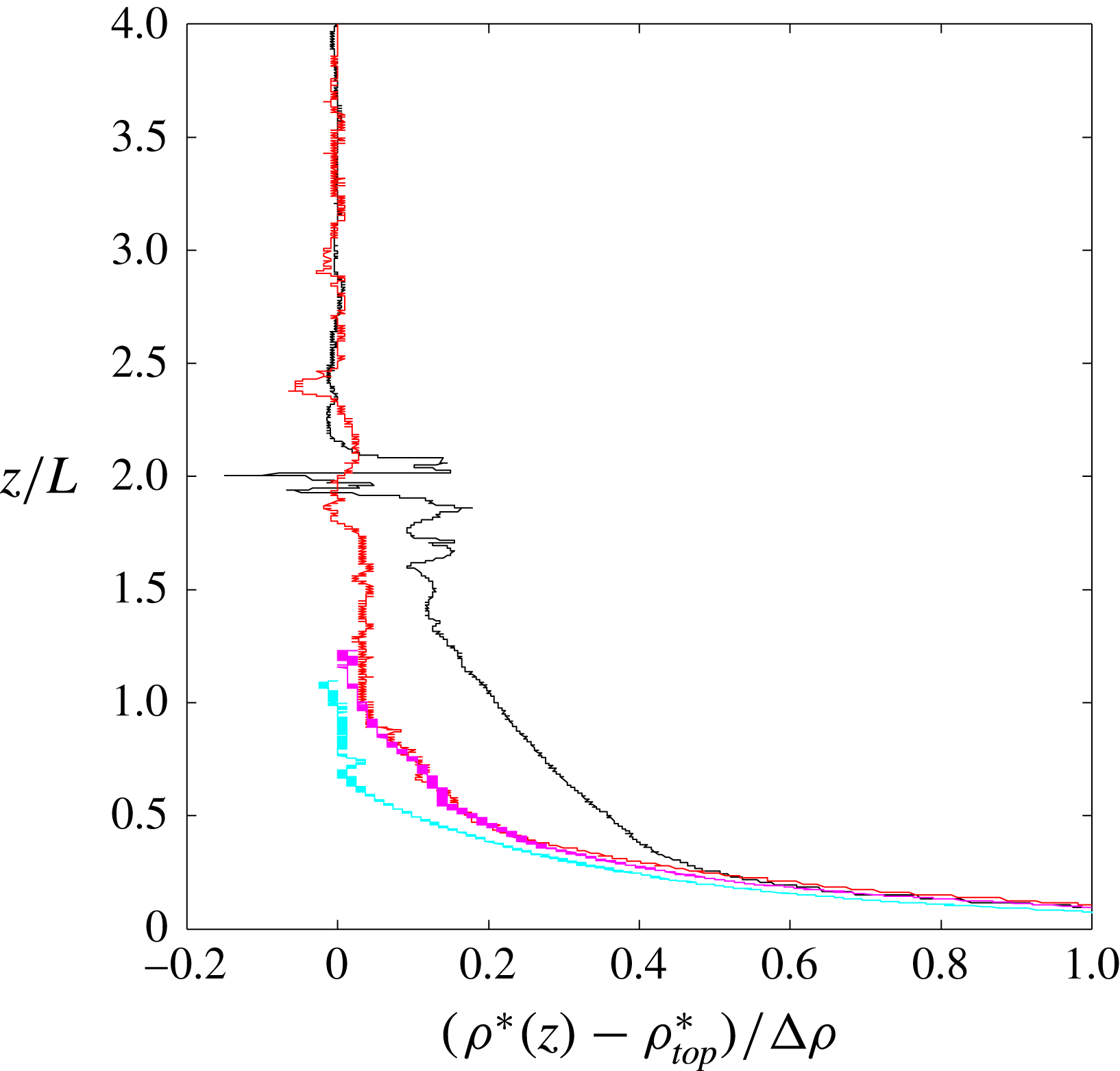
The bulk of the box was always stably stratified (figure 3). As the box freshened with time the density differences in the box increased, at least in a lower region
 $z<L$
above areas of saline input. There the bottom boundary layer thickness (defined as the region containing 90 % of the top-to-bottom density difference, assuming a bottom density equal to the saline input
 $\unicode[STIX]{x1D70C}_{s}$
) was
 $\unicode[STIX]{x1D6FF}\approx 0.1L$
, somewhat thicker than estimated for the viscous boundary layer regime. However, the boundary layer was too thin for much of its profile to be measured. The corresponding buoyancy frequency
 $N=[-(g/\unicode[STIX]{x1D70C}_{0})\,\text{d}\unicode[STIX]{x1D70C}^{\ast }/\text{d}z]^{1/2}$
is over an order of magnitude less than the depth-averaged buoyancy frequency
 $N_{0}=[(g/\unicode[STIX]{x1D70C}_{0})(\unicode[STIX]{x1D70C}_{s}-\unicode[STIX]{x1D70C}_{top}^{\ast })/H]^{1/2}$
throughout most of the depth (
 $1\leqslant z/L\leqslant 3.5$
in the deep cases), and is also consistent with the expectation that the average in the boundary layer will be
 $(N/N_{0})^{2}\sim H/\unicode[STIX]{x1D6FF}\sim 10^{2}$
.
Images of fluorescein dye in the shallow case (exp. 31b,
 $A=2$
,
 $n=4$
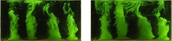
) using illumination of a vertical plane aligned with a row of freshwater input regions and after the densities had been at equilibrium for at least 80 min. Images were taken 60 s apart, approximately 10 min after the dye was added to the freshwater supply manifold.

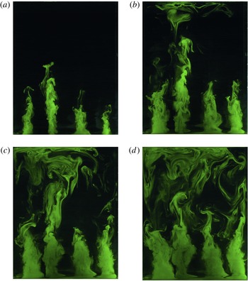
Images of Fluorescein dye injected with the freshwater in the deep case (exp. 18,
 $A=5$
,
 $n=4$
) showing the tracer distribution in the same plane as in figure 4. Images show the flow 140 min after the experiment began and had been in equilibrium for at least 30 min, and approximately 10 min after the dye was added to the freshwater supply manifold. Frames are at intervals of 60 s.

3.2 Flow visualisation
When trace amounts of fluorescein or food dye were added to one of the inputs after the system reached equilibrium, the bottom boundary layer flow could be seen. Over a time much shorter than the equilibration time, tracer in the saline input tended to slowly flood a very thin layer on the permeable plate, of order 2 mm thick. From this sublayer at the bottom of the boundary layer the tracer was carried into the base of plumes as they ascended from the areas of freshwater input. It was not possible to continue the tracer input and retain visible concentration differences for times comparable to the equilibration time, meaning that the full thickness of the boundary layer revealed by the conductivity profiles could not be observed. Addition of fluorescein dye to the fresher input (figures 4 and 5) again showed convergent horizontal flow on the base in the outer parts of each circular area of fresh input, but convective up-flow to heights
 $z/L\sim 1$
over most of the circular patch. The up-flow formed coherent and somewhat turbulent plumes immediately above each of the regions of fresher input. In all shallow-water cases the plumes extended through the full depth (figure 4). Down-flow between the plumes could be seen once tracer began recycling from the top. In the deep-water cases for
 $n=4$
(figure 5) the plumes broke down at a height
 $1<z/L<2$
, above which the tracer showed more disorganised and time-varying motions that included a large box scale of overturning, in which individual plumes on the forcing scale were identifiable only intermittently. No such transition from a fixed array of plumes to large scales was seen for
 $n=3$
, where the square array of coherent plumes was maintained even in deep water (
 $A=5$
).
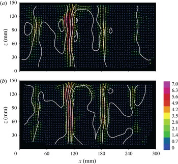
Mean 2D velocity fields and streamfunction at two times for the shallow case
 $A=2$
(exp. 27) on a vertical plane through a row of the freshwater inputs. Fields are temporal averages over
 $3t_{b}$
beginning at
 $t=50$
min (a) and
 $t=80$
min (b). The density reached equilibrium by
 $t=30$
min. Velocity scale (colourbar) is in
 $\text{mm}~\text{s}^{-1}$
; 2D streamfunction contours are at intervals of
 $20~\text{mm}^{2}~\text{s}^{-1}$
.

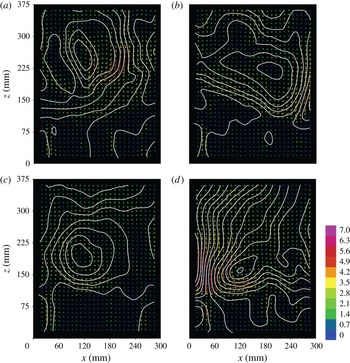
Mean 2D velocity fields and streamfunction at four times for the deep case
 $A=5$
(exp. 13), on the same vertical plane as shown in figure 6 and averaged over 100 s (approximately
 $40t_{b}$
), beginning at (a) 40 min, (b) 45 min, (c) 80 min and (d) 85 min into the experiment. The density reached steady state before
 $t=30$
min. The magnitude of velocity vectors is shown by the colour scale in
 $\text{mm}~\text{s}^{-1}$
; 2D streamfunction is contoured at intervals of
 $30~\text{mm}^{2}~\text{s}^{-1}$
.

3.3 Velocity fields and wavenumbers
Velocity measurements confirm the equilibration of the flow. The temporal average
 $\bar{u}$
,
 $\bar{w}$
of the two-component velocity field over the vertical planar area
 $A$
of the light sheet was calculated over three buoyancy time scales
 $t_{b}$
, and from that the mean flow kinetic energy
 $\bar{E_{k}}$
(
 $\text{J m}^{-1}$
) was found,
 $$\begin{eqnarray}\bar{E_{k}}=\frac{\bar{\unicode[STIX]{x1D70C}}^{\ast }}{2}\int (\bar{u}^{2}+\bar{w}^{2})\,\text{d}A.\end{eqnarray}$$
This measure of the kinetic energy is derived only from the resolved scales, noting that the turbulent kinetic energy of the small scales is not evaluated due to the coarse spatial resolution of the velocity field, and the average over a time window effectively provides the energy of the larger scales of motion. The mean kinetic energy is initially large as a result of net input of buoyancy and decays on a time scale of order
 $10^{3}$
s, which is consistent with the time scale found for density adjustments. At large times the secular trend vanishes. However, the equilibrium continues to show significant variability, reflected in both large standard deviations at time scales less than 300 s and variability between averages over 300–600 s windows, on the order of 50 % of the long-term average kinetic energy. It was confirmed by tracer and PTV results that this variability includes low-frequency reversals of the overturning on the scale of the whole domain.
The velocity fields present a picture of the flow behaviour consistent with that from advection of dye. For the shallow case, as illustrated by 100 s averages in figure 6, the vertical velocity shows maxima in each of the plumes above the regions of destabilising boundary flux, and these maxima are coherent throughout the depth. Between the plumes the flow is predominantly downwards. Although there is some low-frequency fluctuation of the velocity field (as seen over the 55 min between the fields in figure 6) the plume scales of the flow pattern in the shallow case are stationary.
For the deep case (figure 7) velocity maxima and coherent vertical plumes can be associated with only some of the fresher inputs at any one time, only intermittently at any fresh input region, and then only at
 $z<2L$
. Above this level the velocity fields reveal circulation dominated by the scale of the box. This large scale of overturning frequently involves an asymmetry, with regions of faster, narrower flow that can be either upwards or downwards, and broader return flow. Velocities also vary with time, as illustrated by the fields in figure 7: the maximum velocity doubles in the 5 min elapsed between figures 7(c) and 7(d), and the large-scale motion reverses direction (clockwise to anticlockwise) in the 40 min elapsed between figures 7(a,b) and 7(b,c).
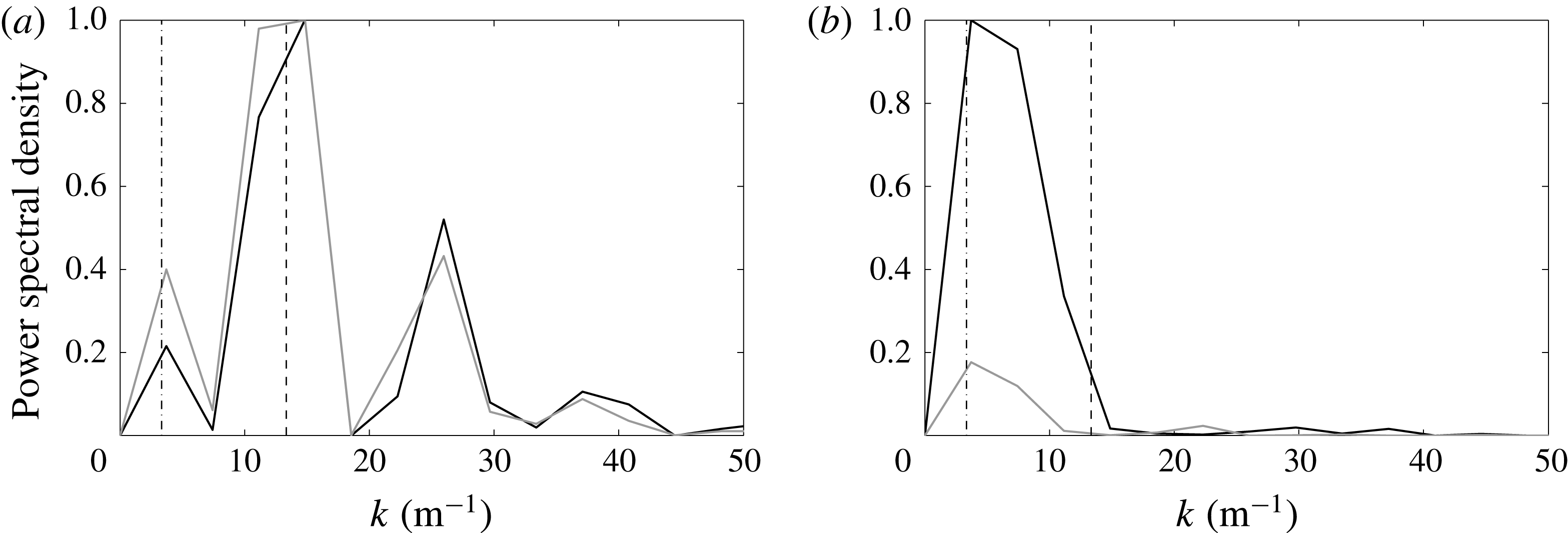
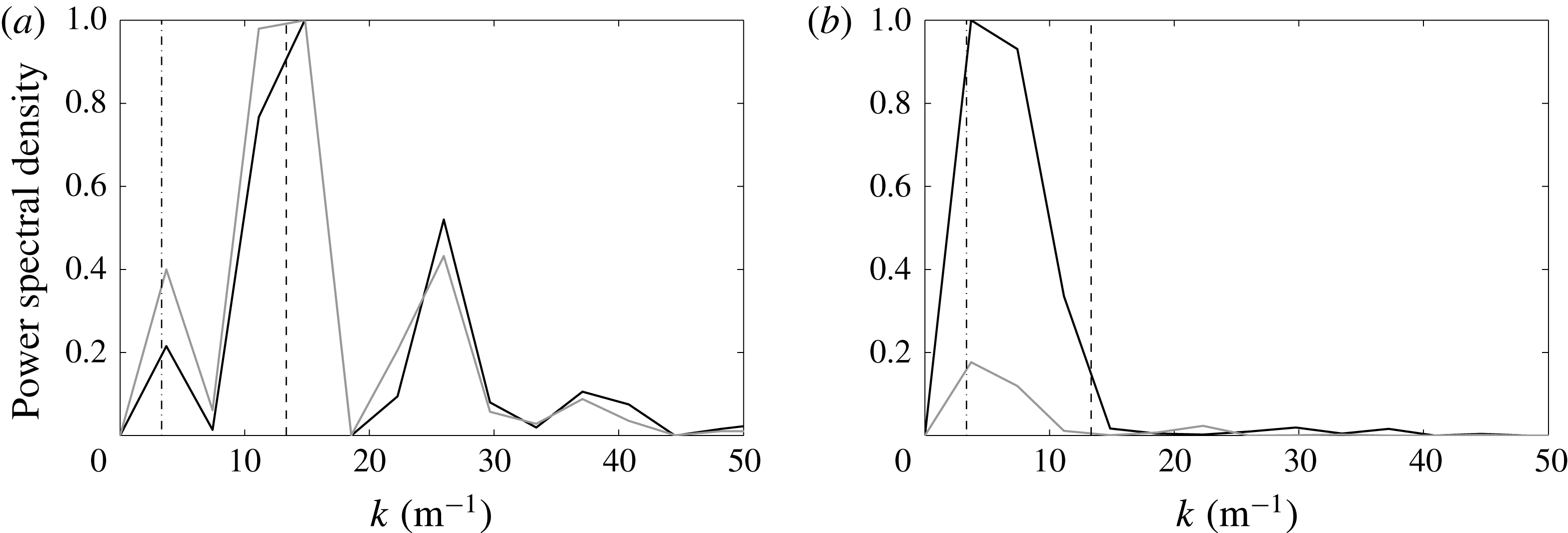
Wavenumber spectra were calculated from a fast Fourier transform of the vertical component
 $w(x)$
of velocity in the illuminated vertical plane at a given time and at several heights. These velocity–wavenumber spectra were computed from frames at ten second intervals and averaged over a ten minute record, and the results in figure 8 are shown (for mid-depth and upper region) normalised by the maximum in power spectral density across all heights. Only wavenumbers
 $0\leqslant k\leqslant 25$
, corresponding to length scales larger than 40 mm, are resolved, as the particle velocity information was binned over 10 mm windows. There was a convincing maximum power at the forcing scale for the shallow case at all heights, with larger scales having power comparable to the small scales. In this case the maximum power in the vertical velocity field occurred near mid-height. In the deep case there was instead a maximum power at the box scale at mid-depth and upper levels. The forcing scale in this case appeared as a peak in the wavenumber spectrum only at small heights, where the power density was also a maximum.
Horizontal wavenumber spectra for (a) shallow (exp. 27) and (b) deep (exp. 30) cases, expressed as the normalised power spectral density of mean kinetic energy. These were found at mid-depth (black line) and at an upper level (grey line); (
 $z/L=1.5$
in (a) and
 $z/L=3.75$
in (b)). The dashed lines correspond to the width of the box (
 $k=1/4L$
) and the forcing scale (
 $k=1/L$
). Dominant peaks are at the forcing scale for the shallow case and at the box scale for the deep case.
3.4 Frequency spectra
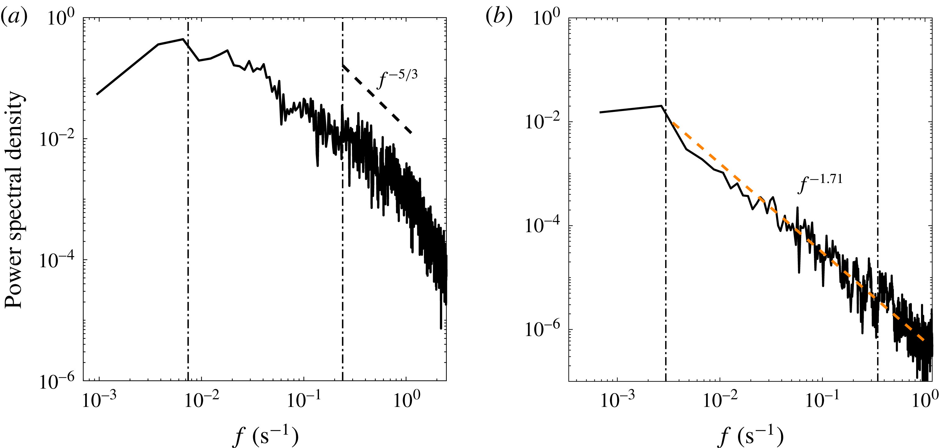
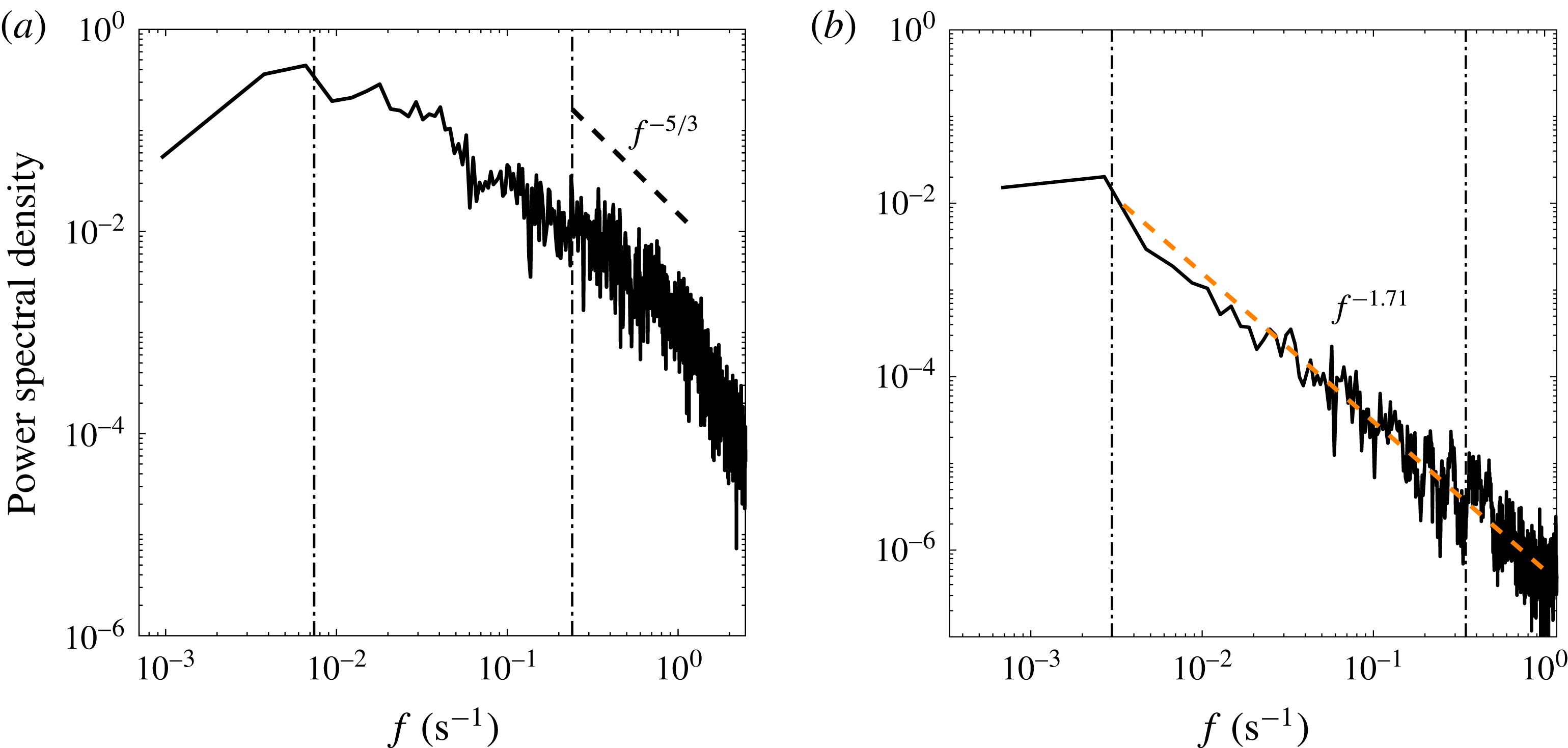
In order to investigate the small scales, frequency spectra were obtained from in situ conductivity fluctuations measured at fixed locations. The conductivity was logged at 10 Hz and the time series spanned the duration of an experiment in cases where only one location was sampled. The record was cut into 1 hr segments, the frequency spectra computed for each segment, and then averaged. In other experiments several records of 30–60 min were obtained at different locations. Spectra for shallow and deep cases are shown in figure 9. Both cases have a maximum power density near frequency
 $U_{0}/(2\unicode[STIX]{x03C0}H)$
(where
 $U_{0}$
is the measured speed of the box scale of motion and
 $H/U_{0}$
is approximately the time for advection of tracer or flow structures through the depth
 $H$
). For the deep case (figure 9
b) the low frequencies, corresponding to fluctuations of the large scales, include the observed translations, rotations and reversals of large overturning cells, whereas in the shallow case (figure 9
a) the low frequencies represent only relatively small variability of the array of discrete plumes about a mean state. Higher frequencies, on the other hand, correspond largely to advection of small-scale structure past the measuring probe. For the shallow cases there is only a narrow range (frequencies greater than approximately
 $H/(2\unicode[STIX]{x03C0}Lt_{b})$
, corresponding to scales a little smaller than
 $L$
) in which the spectral slope is not inconsistent with the
 $-5/3$
expected for an inertial subrange. This is because experiments achieve only modest Reynolds numbers for the discrete plumes. In contrast, for the deep cases the spectrum is in close agreement with a
 $-5/3$
slope across more than two orders of magnitude in frequency, corresponding approximately to length scales ranging from somewhat smaller than the forcing scale
 $L$
up to the domain scale
 $H$
or
 $W$
.
Measured frequency spectra of density fluctuations in experiments, derived from conductivity for (a) a shallow case (
 $A=2$
, at height
 $z=L$
, exp. 28) and (b) a deep case (
 $A=5$
, at
 $z=4L$
, exp. 31). In (a) the spectrum is from a single long record and in (b) it is the average of four 25 min records from different locations in the domain. Spectra have been smoothed by 3-point binning. The vertical lines show
 $H/(2\unicode[STIX]{x03C0}Lt_{b})$
(the higher frequency of the two) and
 $U_{0}/(2\unicode[STIX]{x03C0}H)$
(where
 $U_{0}$
is the measured velocity of the largest scale of motion), which serve to indicate approximate frequencies corresponding to the advection of features having scale
 $L$
and
 $H$
, respectively. The power law slope
 $-5/3$
is shown in (a) for comparison at the frequencies expected of turbulence in discrete plumes; a power law regression fit to frequencies between that of box-scale overturning (vertical line) and
 $f=1~\text{s}^{-1}$
is shown in (b), and gives power
 $-1.71$
.
4 Direct numerical simulations
4.1 Method
In the parallel DNS study of the analogous thermal convection problem we extend the results of Griffiths & Gayen (Reference Griffiths and Gayen2015) by considering a square domain of width
 $W$
and a planar horizontal bottom boundary on which the temperature distribution is imposed as the square array
 $$\begin{eqnarray}T=\unicode[STIX]{x0394}T\sin ^{2}(\unicode[STIX]{x03C0}x/L)\sin ^{2}(\unicode[STIX]{x03C0}y/L),\end{eqnarray}$$
where
 $(x,y)$
are horizontal coordinates with origin at one corner of the domain,
 $\unicode[STIX]{x0394}T$
is the peak-to-peak temperature difference and
 $L$
is the wavelength of the forcing pattern. The domain width is chosen to be an integer number of wavelengths
 $n$
, so that the computational domain is
 $0\geqslant (x,y)\geqslant nL$
. The water depth
 $H$
in this case is such that
 $A=0.5$
or 5, values chosen to most clearly illustrate the difference between shallow and deep cases.
The flow solution is obtained by solving the Navier–Stokes momentum equation in the Boussinesq approximation, assuming incompressibility and a linear equation of state. The flow is fully defined by four dimensionless parameters corresponding to those in (2.1): width of the convection domain and number of hotspots in each direction
 $n$
, the vertical aspect ratio
 $A$
, the Prandtl number
 $Pr=\unicode[STIX]{x1D708}/\unicode[STIX]{x1D705}$
and the Rayleigh number
 $Ra=g\unicode[STIX]{x1D6FC}\unicode[STIX]{x0394}TL^{3}/\unicode[STIX]{x1D705}/\unicode[STIX]{x1D708}$
(based on
 $\unicode[STIX]{x0394}T$
and the forcing scale
 $L$
). Our focus is primarily on the role of the Rayleigh number, a parameter that is difficult to vary significantly in the saline experiments. Different values of
 $Ra$
are achieved by changing the magnitude of the buoyancy forcing
 $g\unicode[STIX]{x1D6FC}\unicode[STIX]{x0394}T$
. The solution is extremely demanding of computational capacity, particularly as a result of the combination of large
 $Ra$
and the lengthy integration to thermal equilibrium in each case (Griffiths et al.
Reference Griffiths, Hughes and Gayen2013). Hence we are restricted to
 $Ra\leqslant 10^{12}$
and
 $n\leqslant 4$
. For this reason solutions were computed for
 $Pr=1$
(which results in the smallest computational time),
 $A=0.5$
and 5 (chosen to be clearly in either the plume regime of the LSC regime), the range of Rayleigh numbers
 $10^{7}\leqslant Ra\leqslant 10^{12}$
, and periodic side boundary conditions (which help reduce the computational time). The top and bottom boundaries are impermeable and no-slip; the top boundary is adiabatic. Comparison with solutions for impermeable, no-slip sidewalls at
 $Ra\leqslant 10^{12}$
were reported in Griffiths & Gayen (Reference Griffiths and Gayen2015) and show qualitatively similar behaviour. (The use of periodic side boundary conditions here should not be confused with the spatially periodic, sinusoidal temperature condition on the base, and the computational domain contains
 $n$
wavelengths of the forcing irrespective of the side boundary conditions.) Each case was initiated with a uniform (relatively cool) fluid temperature and allowed to evolve in time until it reached thermal equilibrium, which was indicated by no long-term secular trend and vanishing net time-averaged heat transport through the bottom boundary.
The numerical methods and tests of the solutions are similar to those reported in previous studies of Rayleigh–Bénard convection (Gayen et al.
Reference Gayen, Hughes and Griffiths2013b
) and the Rossby problem (Griffiths et al.
Reference Griffiths, Hughes and Gayen2013; Gayen et al.
Reference Gayen, Griffiths, Hughes and Saenz2013a
, Reference Gayen, Griffiths and Hughes2014). The grid size
 $\unicode[STIX]{x1D6E5}_{x,y,z}$
in each of
 $x$
,
 $y$
and
 $z$
directions was much smaller in the vicinity of top and bottom boundaries and near the endwall. The grid resolutions for all runs were compared with the Kolmogorov scale,
 $\unicode[STIX]{x1D702}_{K}=(\unicode[STIX]{x1D708}^{3}/\unicode[STIX]{x1D700})^{1/4}$
(where
 $\unicode[STIX]{x1D700}$
is the local viscous dissipation rate and, for
 $Pr\leqslant 1$
,
 $\unicode[STIX]{x1D702}_{K}$
is also the Batchelor microscale) in order to ensure that they satisfied the criteria
 $[\unicode[STIX]{x1D6E5}_{x},\unicode[STIX]{x1D6E5}_{y},\unicode[STIX]{x1D6E5}_{z}]_{max}\leqslant \unicode[STIX]{x03C0}\unicode[STIX]{x1D702}_{K}$
(Stevens, Verzicco & Lohse Reference Stevens, Verzicco and Lohse2010). All results reported here are from runs in which the resolution was significantly better than this criterion. The solution grids used for the deep-water cases therefore had
 $N_{x}\times N_{y}\times N_{z}=1536\times 1536\times 760$
cells for the largest value of
 $Ra$
and
 $256\times 256\times 256$
cells for the smallest value of
 $Ra$
. A low-storage third-order Runge–Kutta–Wray method was used for time stepping, except for the viscous terms, which were treated implicitly using the alternating direction implicit method. The time steps were in all cases an order of magnitude smaller than the minimum Kolmogorov time scale anywhere in the computational domain. Exact closure of the energy budget with each term computed independently is the most stringent test of adequate resolution (Gayen et al.
Reference Gayen, Griffiths, Hughes and Saenz2013a
,Reference Gayen, Hughes and Griffiths
b
) and in the worst case (largest
 $Ra$
) the budget was closed to within 0.14 % of the smallest term (which was the total viscous dissipation rate).
4.2 DNS results
Simulations of the shallow case (
 $A=0.5$
) with
 $n=3$
and
 $n=4$
show a coherent plume ascending above each of the hotspots on the bottom boundary, even at the largest
 $Ra$
, at which each plume is turbulent (a solution for this case with
 $Ra=10^{12}$
is shown in figure 1 of Griffiths & Gayen (Reference Griffiths and Gayen2015) and is not reproduced here). The plumes become turbulent at around
 $Ra\geqslant 10^{9}$
and expand with height as a result of turbulent entrainment of the surrounding fluid. These results are consistent with the saline experiments. For a deep box (
 $A=5$
) and
 $n=3$
the coherent plumes continue to persist in a stable array, again consistent with observations in the analogue experiments.
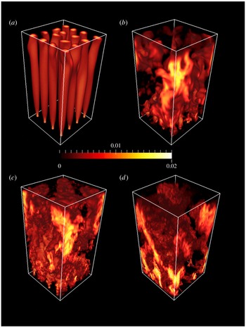
Snapshots of the DNS solutions for
 $n=4$
and deep water (
 $A=5$
) for (a)
 $Ra=10^{7}$
, (b)
 $Ra=10^{8}$
, (c)
 $Ra=10^{9}$
and (d)
 $Ra=10^{12}$
. The three-dimensional renditions show the vertical component of velocity,
 $w$
, in locations where
 $w$
is positive (black where
 $w\leqslant 0$
). Colour scale indicates velocity normalised by
 $(g\unicode[STIX]{x1D6FC}\unicode[STIX]{x0394}TH)^{1/2}$
. See figure 1 of Griffiths & Gayen (Reference Griffiths and Gayen2015) for the shallow-water case corresponding to (d).

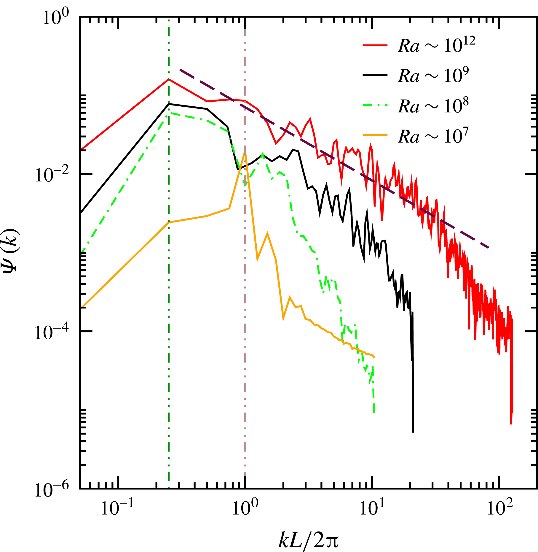
Kinetic energy power spectra for the deep case (
 $A=5$
), with
 $n=4$
at four values of
 $Ra=10^{7}{-}10^{12}$
. The KE is obtained from the three-dimensional DNS velocity field, with velocity normalised by
 $(g\unicode[STIX]{x1D6FC}\unicode[STIX]{x0394}TH)^{1/2}$
, and plotted as a function of horizontal wavenumber
 $k$
(with wavenumber normalised by the forcing wavenumber
 $2\unicode[STIX]{x03C0}/L$
of the forcing). Data are averages over 20 distributed locations in the interior of the flow. Vertical dotted lines show the width of the domain at
 $2\unicode[STIX]{x03C0}/L=0.25$
. A
 $-5/3$
slope (broken line) describes the spectrum for
 $Ra=10^{12}$
over the wavenumber range
 $0.25\leqslant kL/2\unicode[STIX]{x03C0}\leqslant 30$
.

In contrast, the deep case with
 $n=4$
shows a flow field that changes dramatically with Rayleigh number. At
 $Ra=10^{7}$
the velocity field (figure 10
a, here normalised by the inertial-buoyancy velocity scale
 $\sqrt{g\unicode[STIX]{x1D6FC}\unicode[STIX]{x0394}TH}$
) shows an array of discrete, almost steady plumes in which the fluid ascends vertically above each hot patch. The plumes remain stable in a square array, although the upper portion of the columnar structures shows a small unsteadiness, the first signs of plume–plume interactions. At this
 $Ra$
the flow is completely laminar, as is also revealed from the kinetic energy spectrum (figure 11), which shows a sharp decay of energy on each side of a peak at the forcing length scale. At
 $Ra\sim 10^{8}$
(figure 10
b) the plumes interact more obviously with each other and, as a result, there is significant energy at length scales up to the domain width, with a maximum in the energy spectrum (figure 11) at
 $4L$
rather than at the forcing scale. This implies an upscale energy transfer. The emergent large-scale circulation tends to organise the smaller scales, acts as a mean ‘wind’ and sweeps plumes into quasi-two-dimensional structures. At
 $n=4$
and
 $A=5$
the flow at
 $Ra=10^{8}$
is unsteady, but there is not a well-developed turbulent energy cascade to small scales.
At
 $Ra=10^{9}$
(figure 10
c) there is again a spectral peak at the box scale, but more small-scale turbulence kinetic energy is evident. The spectrum (figure 11) is consistent with a
 $-5/3$
power law expected for the Kolmogorov inertial turbulence subrange, over one order of magnitude in wavenumber, along with a steeper dissipation range at small scales extending to the Kolmogorov scale. At
 $Ra=10^{12}$
the flow is little further changed apart from evidence of still smaller scales and a significant broadening of the inertial turbulence subrange, which now extends over two orders of magnitude in wavenumber. This change in the smallest scales accurately reflects the predicted dependence of the average Kolmogorov scale on Rayleigh number (
 $\unicode[STIX]{x1D702}_{K}\sim L(H/L)^{1/4}Pr^{1/2}Ra^{-1/4}$
). There is greater intermittency in the warm plumes near the bottom boundary; the large scales involve sweeping motions that tend to carry the warm fluid away from the hotspots of the base, collecting it into one or two updraughts. In contrast to flow in the Rossby problem, where vertical motions are highly asymmetric, the present arrangement shows comparable dimensions and speeds for the large updraughts and downdraughts. This symmetry is also apparent in the saline laboratory experiments reported here.
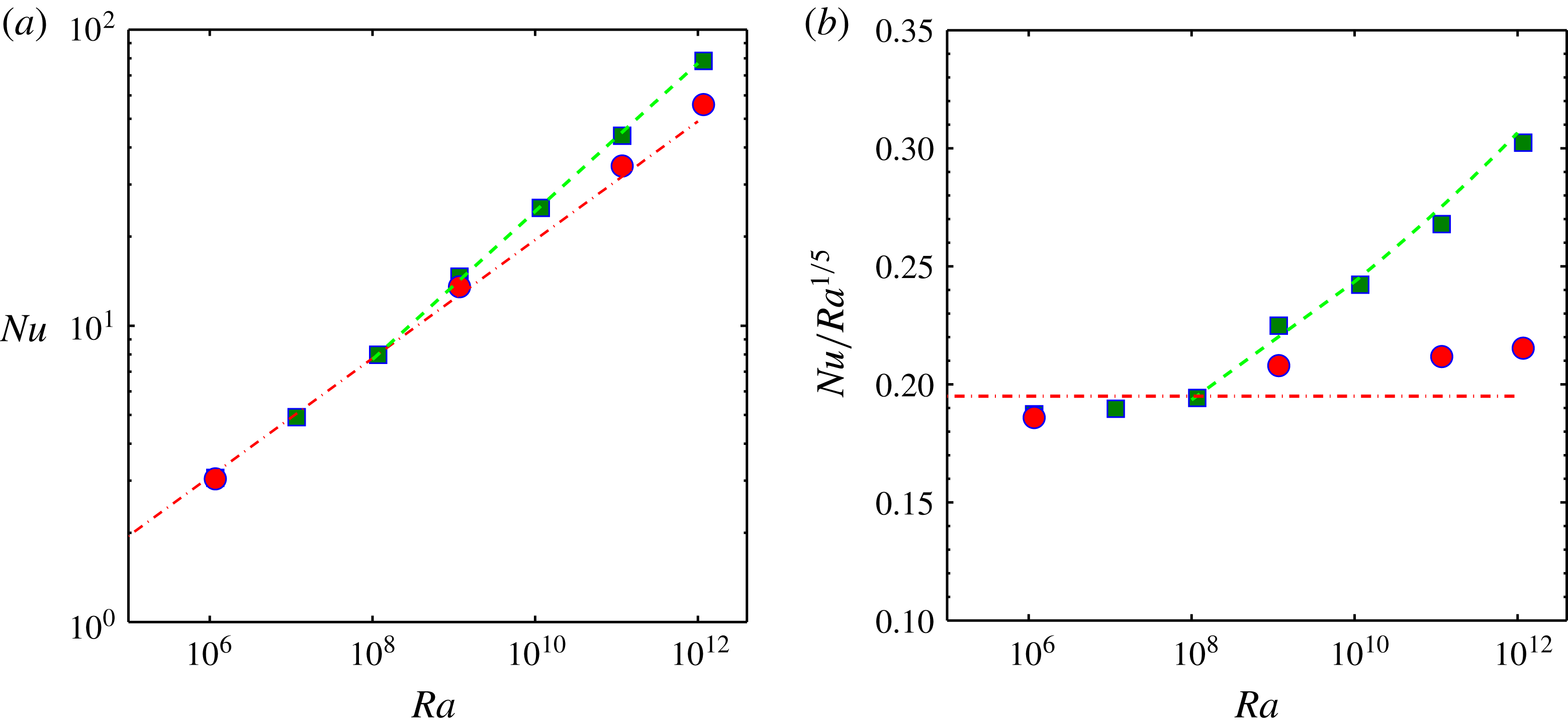
(a) Dimensionless heat transport
 $Nu$
as a function of
 $Ra$
from DNS for the shallow-water (red circles) and deep-water (green squares) cases. Lines show
 $Nu=0.195\,Ra^{1/5}$
(red dashed) and
 $Nu=0.08\,Ra^{1/4}$
(green dashed). The red line is extrapolated to larger values of
 $Ra$
only as a reference and does not represent a single asymptotic similarity regime. In (b) the heat fluxes from (a) are renormalised as
 $Nu/Ra^{1/5}$
and lines corresponding to those in (a) are replotted.

The normalised heat flux (Nusselt number) was estimated from
 $$\begin{eqnarray}Nu=QL/\unicode[STIX]{x1D70C}c_{p}\unicode[STIX]{x1D705}a_{+}\unicode[STIX]{x0394}T=\left.\left[L\int _{a_{+}}\overline{\unicode[STIX]{x2202}T/\unicode[STIX]{x2202}z}|_{z=0}\,\text{d}a\right]\!\right/\![a_{+}\unicode[STIX]{x0394}T],\end{eqnarray}$$
where
 $\unicode[STIX]{x1D70C}_{0}$
is a reference density,
 $c_{p}$
is the specific heat, the (dimensional) heat input is
 $Q=\unicode[STIX]{x1D70C}_{0}c_{p}\unicode[STIX]{x1D705}\int _{a_{+}}\overline{\unicode[STIX]{x2202}T/\unicode[STIX]{x2202}z}|_{z=0}\,\text{d}a$
, the overbar indicates time average and
 $a_{+}$
is the area over which the vertical temperature gradient on the base is positive (i.e. the cooling area). The results (figure 12) indicate that there are at least two, and arguably three, heat transport regimes. At
 $Ra\leqslant 10^{8}$
the flow is laminar and the Nusselt numbers for both shallow and deep cases are consistent with
 $Nu\sim 0.195\,Ra^{1/5}$
, which is the Rossby boundary layer scaling for steady, viscous convection (found at
 $Ra\leqslant 10^{9}$
in the Rossby problem).
For
 $Ra\geqslant 10^{9}$
the results depend on water depth. In the shallow case there is a small increase in the heat transport, consistent with a gradual transition, as found in the Rossby problem at
 $10^{10}\leqslant Ra\leqslant 10^{11}$
(Gayen et al.
Reference Gayen, Griffiths and Hughes2014), towards a turbulent inertial regime in which flow becomes governed by turbulent Reynolds stress in the boundary layer. (We do not examine here the effects of radial flow of the boundary layer into each ascending plume as compared with the rectangular geometry in the Rossby problem.) This regime again yields the
 $1/5$
scaling (but with a larger pre-factor than the viscous regime).
For the deep case the heat transport at
 $Ra\geqslant 10^{9}$
(figure 12) departs markedly from the
 $Ra^{1/5}$
scaling. The results are described very well by
 $Nu\sim 0.08\,Ra^{1/4}$
across four orders of magnitude in
 $Ra$
. The pre-factor is expected to depend on
 $n$
,
 $A$
and
 $Pr$
. The occurrence of the
 $1/4$
scaling is coincident with conditions under which scales of motion larger than the forcing and comparable to the width of the box emerge from the turbulence. The larger scales can more rapidly release available potential energy to motion, and transport heat more rapidly, than do the smaller scales. The transition between regimes for
 $n=4$
and
 $A=5$
lies at
 $Ra\approx 10^{8}$
, where we observe the beginning of strong interactions between the discrete plumes (figure 10
b,c).
Closely related to the heat transport is the generation of available potential energy by the boundary heating and cooling, at the (time-averaged) rate
 $\unicode[STIX]{x1D6F7}_{b2}=\unicode[STIX]{x1D705}g\int _{S}\overline{z^{\ast }\unicode[STIX]{x2202}\unicode[STIX]{x1D70C}/\unicode[STIX]{x2202}z}|_{z=0}\,\text{d}S$
, where
 $S$
is the surface area of the boundary and
 $z^{\ast }$
is the height at which each parcel of fluid would lie if the fluid were reorganised adiabatically into the state of gravitational equilibrium (Winters et al.
Reference Winters, Lombard, Riley and D’Asaro1995; Hughes et al.
Reference Hughes, Hogg and Griffiths2009). A suitable normalisation of this (and other terms in the mechanical energy budget, as discussed below) is a comparison with the rate of viscous dissipation of kinetic energy, the time-averaged box total of which is given by
 $\unicode[STIX]{x1D700}_{T}=\unicode[STIX]{x1D70C}_{0}\unicode[STIX]{x1D708}\int _{V}\overline{\Vert \unicode[STIX]{x1D735}\boldsymbol{u}\Vert ^{2}}\,\text{d}V$
, where
 $V$
is the total volume of the convecting fluid. The APE generation rate normalised by
 $\unicode[STIX]{x1D700}_{T}$
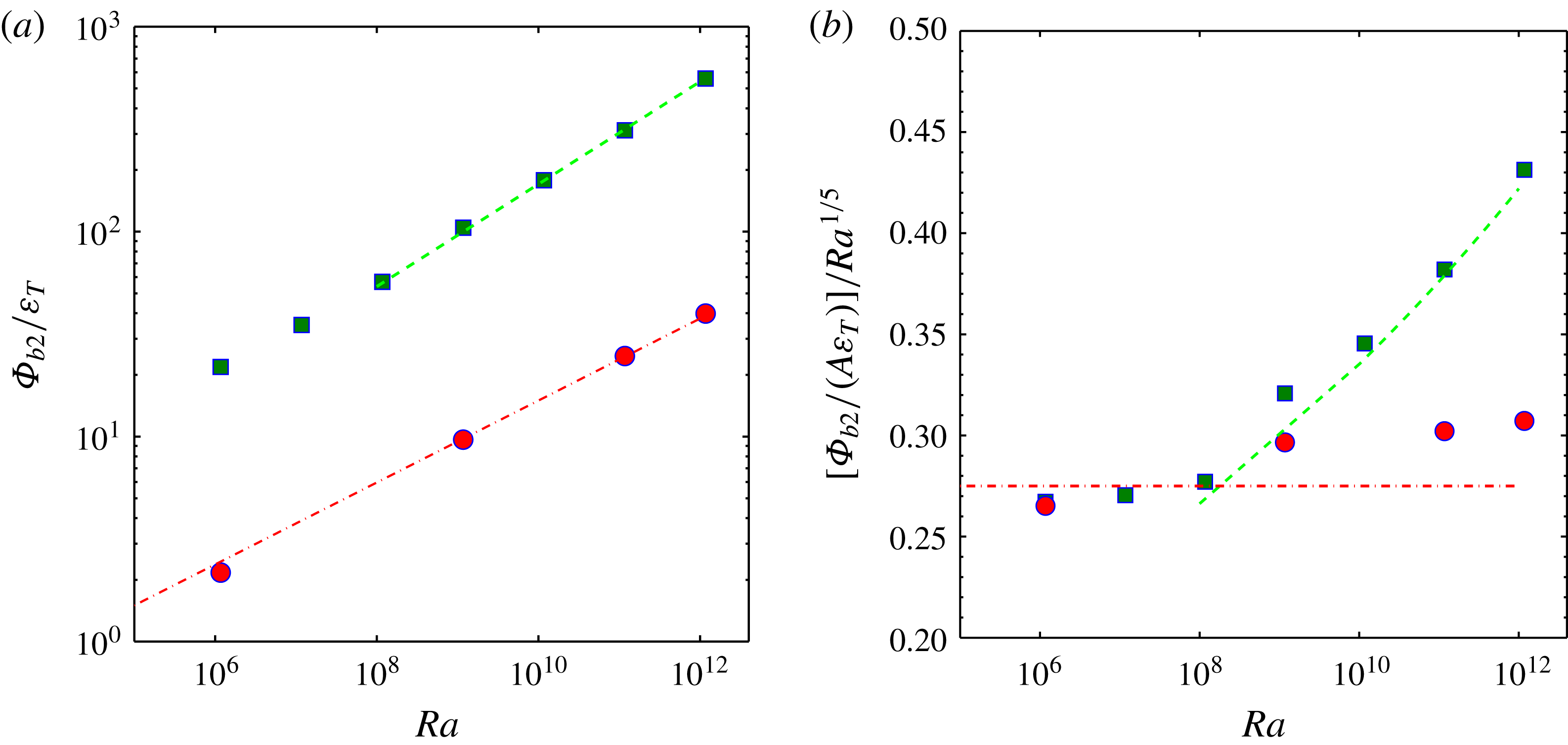
, shown in figure 13(a), increases with both
 $Ra$
and the depth
 $H$
. APE generation reaches approximately 40 (shallow case) and 600 times (deep case) the viscous dissipation.
(a) The rates of generation of available potential energy,
 $\unicode[STIX]{x1D6F7}_{b2}$
, by boundary buoyancy forcing, normalised by the total viscous dissipation rate integrated over the domain volume, as functions of
 $Ra$
from DNS for the shallow-water (red circles) and deep-water (green squares) cases. Lines show the power laws
 $\unicode[STIX]{x1D6F7}_{b2}/\unicode[STIX]{x1D716}_{T}\sim Ra^{1/5}$
(red) and
 $Ra^{1/4}$
(green). In (b) the values from (a) are renormalised by
 $ARa^{1/5}$
(where
 $A=H/L$
) and lines corresponding to those in (a) are replotted.

The trends in APE generation are better represented by the renormalised form shown in figure 12(b), which is based on the following scaling. Considering the hypothetical re-sorting of fluid elements required to define APE, in which the cold boundary layer fluid stays at the base and the hottest fluid goes to the top, we rewrite the above definition of APE generation by surface buoyancy forcing as
 $\unicode[STIX]{x1D6F7}_{b2}\approx \unicode[STIX]{x1D705}g\unicode[STIX]{x1D6FC}\langle \overline{\text{d}T/\text{d}z}|_{-}\rangle a_{-}H$
, where the subscript ‘-’ indicates the boundary temperature gradient in the region of negative vertical temperature gradient at the boundary (i.e. the heating area
 $a_{-}$
), the overbar represents time average,
 $\langle \cdot \rangle$
indicates horizontal averaging over the relevant area and we recognise that
 $|z^{\ast }|\approx H$
. Since heat input is equal to heat withdrawal this can be expressed as
 $\unicode[STIX]{x1D6F7}_{b2}=\unicode[STIX]{x1D705}g\unicode[STIX]{x1D6FC}\unicode[STIX]{x0394}T[L\langle \overline{(\text{d}T/\text{d}z)}|_{+}\rangle /\unicode[STIX]{x0394}T](H/L)a_{+}$
. The normalisation of this quantity is based on the viscous dissipation rate in horizontal convection, which is equal to the rate of generation of potential energy
 $\unicode[STIX]{x1D6F7}_{i}$
(
 $\unicode[STIX]{x1D700}_{T}=\unicode[STIX]{x1D6F7}_{i}$
), which is bounded by
 $\unicode[STIX]{x1D6F7}_{i}\approx -g\unicode[STIX]{x1D705}(\langle \unicode[STIX]{x1D70C}\rangle _{H}-\langle \unicode[STIX]{x1D70C}\rangle _{0})a_{T}$
, where
 $a_{T}$
the horizontal area of the domain and horizontal averaging of density is at the top (
 $z=H$
) and bottom (
 $z=0$
) of the domain (Paparella & Young Reference Paparella and Young2002; Hughes et al.
Reference Hughes, Hogg and Griffiths2009). The computed total dissipation rate in DNS is not measurably different from this upper bound (Gayen et al.
Reference Gayen, Griffiths and Hughes2014; Griffiths & Gayen Reference Griffiths and Gayen2015) and we expect the same expression to hold in the case of the present array forcing. (It was reported in Griffiths & Gayen (Reference Griffiths and Gayen2015) that periodic side boundary conditions gave
 $\unicode[STIX]{x1D700}_{T}$
larger than
 $\unicode[STIX]{x1D6F7}_{i}$
. However, this was due to an error in the normalisation of the integrated dissipation rate. The computed total dissipation is actually indistinguishable from
 $\unicode[STIX]{x1D6F7}_{i}$
for both types of boundary conditions.) Working from
 $\unicode[STIX]{x1D6F7}_{i}$
, it can be shown that the total viscous dissipation rate is
 $\unicode[STIX]{x1D700}_{T}\approx g\unicode[STIX]{x1D705}\unicode[STIX]{x1D70C}_{0}\unicode[STIX]{x1D6FC}\unicode[STIX]{x0394}Ta_{+}$
, or equivalently
 $\unicode[STIX]{x1D700}_{T}\sim (\unicode[STIX]{x1D70C}_{0}\unicode[STIX]{x1D705}^{3}a_{+}/L^{3})(Ra\,Pr)$
. The normalised APE generation rate becomes
 $$\begin{eqnarray}\unicode[STIX]{x1D6F7}_{b2}/\unicode[STIX]{x1D700}_{T}\sim ANu,\end{eqnarray}$$
which is identical to the previous theoretical scaling proposed for the rectangular Rossby problem (Gayen et al.
Reference Gayen, Griffiths, Hughes and Saenz2013a
) and found to be a robust result (Gayen et al.
Reference Gayen, Griffiths and Hughes2014; Vreugdenhil et al.
Reference Vreugdenhil, Gayen and Griffiths2016). In comparison to the heat transport
 $Nu$
, APE generation has an additional dependence on water depth
 $H$
(or the aspect ratio
 $A$
), as a result of gravitational potential. Thus the DNS results are renormalised in figure 12(b) as
 $\unicode[STIX]{x1D6F7}_{b2}/(\unicode[STIX]{x1D700}_{T}ARa^{1/5})$
and the results closely mirror the trends in renormalised Nusselt number,
 $Nu/Ra^{1/5}$
(figure 12
b).
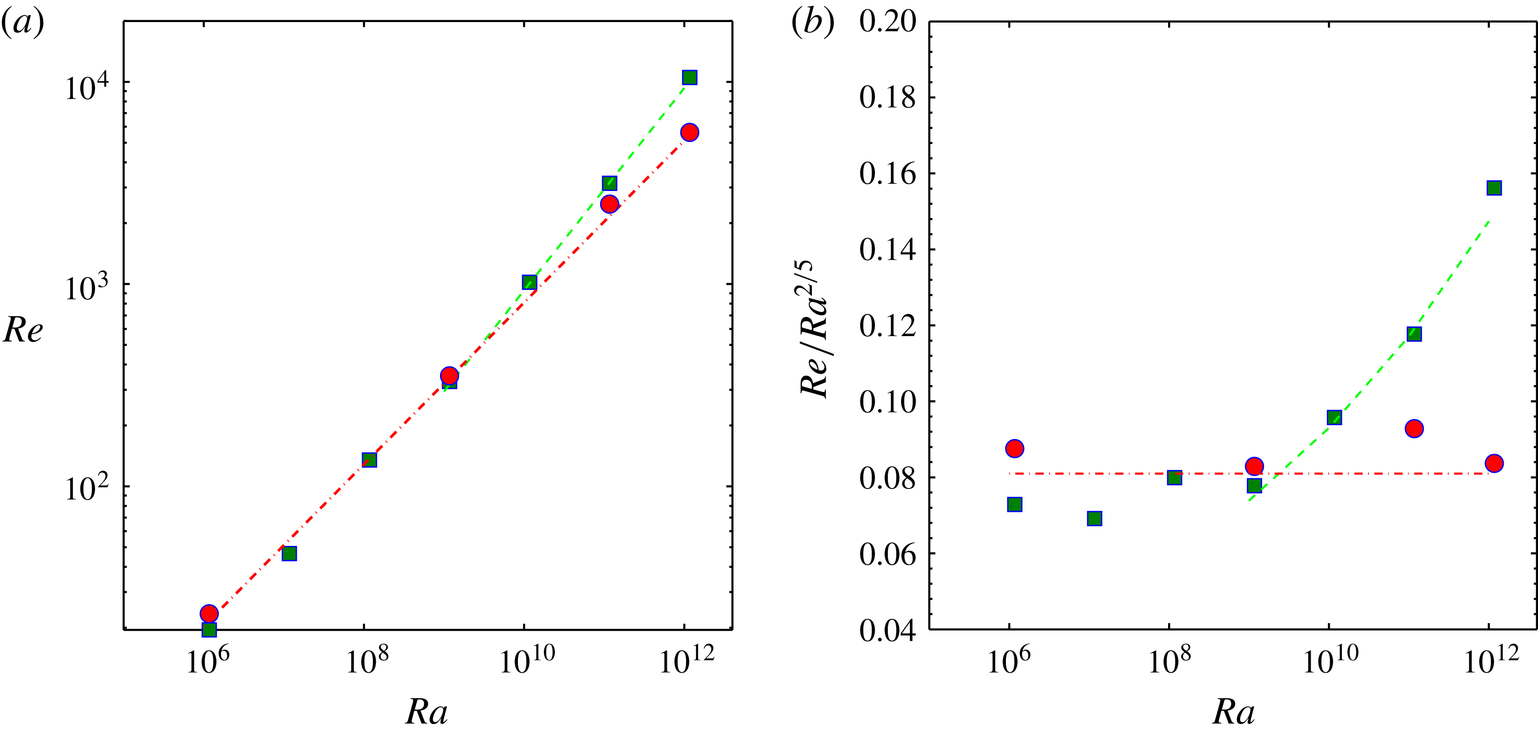
The flow velocities are represented in figure 14 as the Reynolds number
 $Re=UL/\unicode[STIX]{x1D708}$
, which is evaluated from the root-mean-square magnitude of velocities within the volume of the thermal boundary layer (defined, as before, by
 $z<\unicode[STIX]{x1D6FF}$
, where
 $\unicode[STIX]{x1D6FF}$
encompasses 95 % of the horizontally averaged bottom-to-top temperature difference). Again these velocities show at least two regimes: the deep-water case at
 $Ra>10^{8}$
diverges markedly from all other cases and is characterised by larger velocities.
Reynolds number
 $Re=UL/\unicode[STIX]{x1D708}$
(a) based on the boundary layer velocity computed from the kinetic energy,
 $U=\langle (u^{2}+v^{2}+w^{2})/2\rangle ^{1/2}$
, and averaged over the volume of the boundary layer, shown as a function of Rayleigh number, from DNS for the shallow-water (red circles) and deep-water (green squares) cases. Lines show the power laws
 $Re\sim Ra^{2/5}$
(red) and
 $Re\sim Ra^{1/2}$
(green). In (b) the values from (a) are normalised by
 $Ra^{2/5}$
and lines corresponding to those in (a) are replotted.

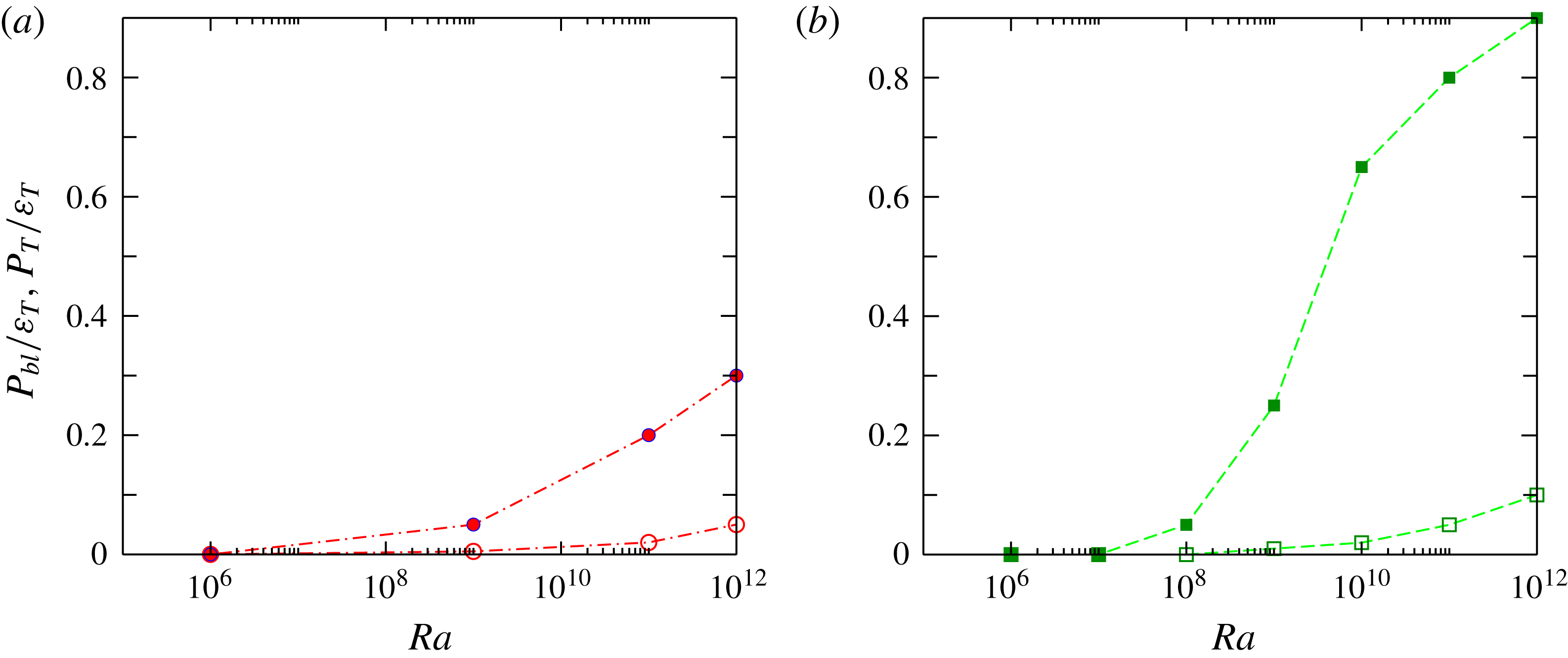
Volume-integrated shear production rates
 $P$
(conversion of mean to turbulent kinetic energy) as functions of Rayleigh number from DNS for the (a) shallow-water and (b) deep-water cases. TKE production rate is integrated over the volume of the thermal boundary layer (open symbols) or the whole domain (filled symbols), and normalised by the total domain-integrated viscous dissipation rate.

The Rayleigh number dependence of the shear production
 $P=-\unicode[STIX]{x1D70C}_{0}\sum _{i,j=1}^{3}\overline{u_{i}^{\prime }u_{j}^{\prime }}(\unicode[STIX]{x2202}\overline{u}_{i}/\unicode[STIX]{x2202}x_{j})$
(where overbars again represent time averages), when integrated over both the full volume of the domain,
 $P_{T}=\int _{V}P\,\text{d}V$
, is shown in figure 15, where it is given as a fraction of the total viscous dissipation rate
 $\unicode[STIX]{x1D716}_{T}$
. For comparison, the proportion of
 $P_{T}$
found in the boundary layer,
 $P_{bl}$
, is also shown. Shear production is insignificant in the viscous regime at
 $Ra<10^{8}$
. Shear production grows to 30 % (shallow case) or 90 % (deep case) of the total kinetic energy production (and dissipation) rate at
 $Ra=10^{12}$
. At this Rayleigh number the interior accounts for most of the shear production in both cases (approximately 83 % in the shallow case and 89 % in the deep case). Thus the boundary layer accounts for a small fraction of the shear production (and viscous dissipation) under all conditions. The bottom boundary layer at
 $Ra=10^{12}$
also has a logarithmic profile of the horizontal velocity (Griffiths & Gayen Reference Griffiths and Gayen2015), consistent with shear production within the boundary layer. However, the very small volume of the boundary layer leaves the viscous dissipation almost entirely in the interior.
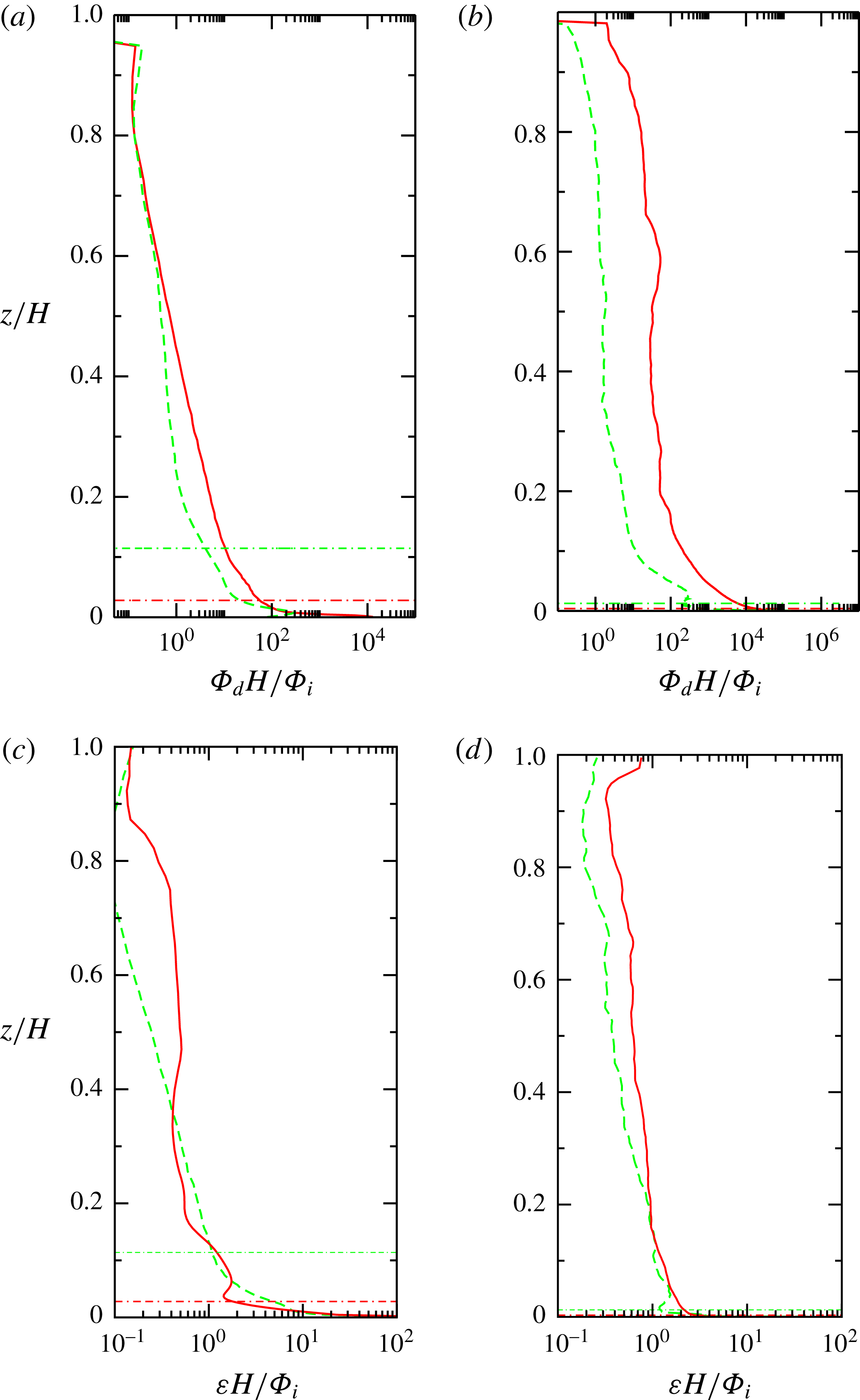
Profiles of irreversible mixing rate
 $\unicode[STIX]{x1D6F7}_{d}$
(a,b) and viscous dissipation rate (c,d) with height for
 $Ra=10^{9}$
(green line) and
 $10^{12}$
(red line) from DNS of the (a,c) shallow-water (
 $H/L=0.5$
) and (b,d) deep-water (
 $H/L=5$
) cases. The computed energy dissipations per unit volume are averaged in time and integrated over the horizontal area
 $W^{2}$
of the domain at each depth, then normalised by the total rate of generation of potential energy
 $\unicode[STIX]{x1D6F7}_{i}$
divided by the domain depth
 $H$
. Horizontal lines show the edge of the thermal boundary layer (
 $\unicode[STIX]{x1D6FF}/H\approx 0.002$
for the deep case at
 $Ra=10^{12}$
). The boundary layer
 $\unicode[STIX]{x1D6FF}$
is defined as the layer containing 95 % of the mean temperature difference: at
 $z=\unicode[STIX]{x1D6FF}$
the horizontally averaged temperature
 $\langle T\rangle =\langle T\rangle _{H}+0.05(\langle T\rangle _{H}-\langle T\rangle _{0})$
.

In contrast with the viscous dissipation is the behaviour of the other sink in the mechanical energy equations: the irreversible mixing
 $\unicode[STIX]{x1D6F7}_{d}=-g\unicode[STIX]{x1D705}\int \overline{(\text{d}z^{\ast }/\text{d}\unicode[STIX]{x1D70C})|\unicode[STIX]{x1D735}\unicode[STIX]{x1D70C}|^{2}}\,\text{d}V$
(Winters et al.
Reference Winters, Lombard, Riley and D’Asaro1995; Hughes et al.
Reference Hughes, Hogg and Griffiths2009). Figure 16 shows the mixing and viscous dissipation rates as depth profiles of the horizontally integrated
 $\unicode[STIX]{x1D6F7}_{d}$
and
 $\unicode[STIX]{x1D700}$
normalised by
 $\unicode[STIX]{x1D6F7}_{i}/H$
(
 $=\unicode[STIX]{x1D700}_{T}/H$
) for two values of the Rayleigh number. For the shallow case (figure 16
a,c) there is not much difference between
 $Ra=10^{9}$
and
 $Ra=10^{12}$
in either the overall (normalised) mixing rate or its distribution. The mixing rates are of
 $O(1)$
in the interior and
 $O(10^{4})$
in the thermal boundary layer. Thus for the shallow cases the mixing rates in the interior are similar to the viscous dissipation rates, whereas mixing in the boundary layer is much larger than both the average and local dissipation rates. Most of the mixing is within the volume of the boundary layer (in line with previous results for the Rossby problem, Gayen et al.
Reference Gayen, Griffiths and Hughes2014). For the deep case (figure 16
b,d), on the other hand, the normalised mixing rates depend more strongly on Rayleigh number. For
 $Ra=10^{9}$
mixing is not much greater than in the shallow case, but at
 $Ra=10^{12}$
the mixing rates are two orders of magnitude greater. The mixing rate is again
 $10^{3}{-}10^{4}$
times greater in the boundary layer than in the interior, giving a preponderance of mixing in the boundary layer volume, despite the thinness of the boundary layer. Vertical integrations show that the confinement of mixing to the boundary layer is stronger for the deep case with larger
 $Ra$
. Also in this case, integration over the whole domain gives a mixing rate approximately 600 times the integrated viscous dissipation. The DNS confirms that the APE budget is dominated by an exact balance,
 $$\begin{eqnarray}\unicode[STIX]{x1D6F7}_{b2}=\unicode[STIX]{x1D6F7}_{d},\end{eqnarray}$$
between the rate of energy supply by the surface buoyancy fluxes and its conversion to background potential energy by irreversible mixing, as predicted by Hughes et al. (Reference Hughes, Hogg and Griffiths2009) and Tailleux (Reference Tailleux2009).
5 Discussion
The experiments and simulations indicate that two-dimensional spatially periodic forcing for
 $Ra>10^{8}$
,
 $n=4$
and
 $H>2L$
leads to flow in which there is transfer of kinetic energy to length scales larger than the forcing. The presence of the large scales leads to enhanced heat transport, which in turn gives enhanced generation of APE by the boundary buoyancy forcing. The energetic large scales also enhance the shear production of small scales. This leads to a greater dominance of the interior over the boundary layer contribution to total viscous dissipation, relative to that previously shown for the turbulent boundary layer regime in the Rossby problem (Gayen et al.
Reference Gayen, Griffiths and Hughes2014). Irreversible mixing, on the other hand, remains strongly confined to the boundary layer, where temperature gradients are much larger than in the interior (Gayen et al.
Reference Gayen, Griffiths, Hughes and Saenz2013a
, Reference Gayen, Griffiths and Hughes2014).
Existing horizontal convection scaling analyses, based on boundary layer dynamics and an imposed temperature difference, are briefly recalled below. These analyses explain two of the regimes observed for the present array forcing: the laminar regime and the array of turbulent plumes in a stable configuration. A scaling analysis is then developed for horizontal convection with a governing momentum balance in the interior large-scale circulation, and where this interior flow is coupled to buoyancy transport through the cooled, gravitationally stable portions of the boundary layer.
The vorticity and heat equations can be written in terms of the streamfunction (Rossby Reference Rossby1965; Gayen et al. Reference Gayen, Griffiths and Hughes2014):
 $$\begin{eqnarray}\displaystyle & J_{\unicode[STIX]{x1D6F9},\unicode[STIX]{x1D6FB}^{2}\unicode[STIX]{x1D6F9}}(x,z)-g\unicode[STIX]{x1D6FC}T_{x}+\unicode[STIX]{x1D708}\unicode[STIX]{x1D6FB}^{4}\unicode[STIX]{x1D6F9}=0, & \displaystyle\end{eqnarray}$$
 $$\begin{eqnarray}\displaystyle & J_{\unicode[STIX]{x1D6F9},T}(x,z)+\unicode[STIX]{x1D705}\unicode[STIX]{x1D6FB}^{2}T=0, & \displaystyle\end{eqnarray}$$
where
 $x$
is the horizontal direction,
 $\unicode[STIX]{x1D6F9}$
is the streamfunction defined by (
 $u=\unicode[STIX]{x2202}\unicode[STIX]{x1D6F9}/\unicode[STIX]{x2202}z$
,
 $w=-\unicode[STIX]{x2202}\unicode[STIX]{x1D6F9}/\unicode[STIX]{x2202}x$
),
 $\unicode[STIX]{x1D6FB}^{2}\unicode[STIX]{x1D6F9}$
is the vorticity and
 $J$
is the Jacobian. Here the slowly varying large-scale (mean) flow is treated as quasi-steady and quasi-two-dimensional. Although the streamfunction formulation is two-dimensional (and as such cannot be used to evaluate flow quantities), scaling of the momentum equation itself would require additional assumptions (Rossby Reference Rossby1965) and the streamfunction approach is necessary in order to obtain unambiguous results when the gravitational acceleration is normal to the direction of the imposed temperature gradient.
Scaling mass, length, time and temperature by
 $\unicode[STIX]{x1D70C}_{0}L^{3}$
,
 $L$
,
 $L^{2}/\unicode[STIX]{x1D705}$
and
 $\unicode[STIX]{x0394}T=T_{h}-T_{c}$
, respectively, the dimensionless form of the above equations is:
 $$\begin{eqnarray}\displaystyle & \overbrace{J_{\hat{\unicode[STIX]{x1D6F9}},\unicode[STIX]{x1D6FB}^{2}\hat{\unicode[STIX]{x1D6F9}}}(\hat{x},\hat{z})}^{\text{inertia terms}}-\overbrace{Pr\,Ra\hat{T}_{\hat{x}}}^{\text{buoyancy terms}}+\overbrace{Pr\unicode[STIX]{x1D6FB}^{4}\hat{\unicode[STIX]{x1D6F9}}}^{\text{viscous terms}}=0, & \displaystyle\end{eqnarray}$$
 $$\begin{eqnarray}\displaystyle & \overbrace{J_{\hat{\unicode[STIX]{x1D6F9}},\hat{T}}(\hat{x},\hat{z})}^{\text{advection terms}}+\overbrace{\unicode[STIX]{x1D6FB}^{2}\hat{T}}^{\text{diffusion terms}}=0, & \displaystyle\end{eqnarray}$$
where dimensionless quantities are indicated by a hat,
 $\hat{\unicode[STIX]{x1D6F9}}_{z}=\hat{u}$
and
 $\hat{\unicode[STIX]{x1D6F9}}_{x}=-{\hat{w}}$
.
5.1 Boundary layer viscous–buoyancy balance
Rossby (Reference Rossby1965, Reference Rossby1998) developed a boundary layer analysis of horizontal convection due to a one-directional gradient of boundary temperature over the length
 $L$
of a closed box, assuming thermal boundary layer thickness
 $\unicode[STIX]{x1D6FF}\ll L$
,
 $H$
, that the flow is governed by viscous stress and that effects of inertia are assumed negligible. Under these assumptions it was argued that the thermal and velocity boundary layer thicknesses have the same scaling, while vertical derivatives in the boundary layer are the dominant contributions (
 $\unicode[STIX]{x2202}/\unicode[STIX]{x2202}z\gg \unicode[STIX]{x2202}/\unicode[STIX]{x2202}x$
) to both the viscous drag (
 ${\sim}\unicode[STIX]{x1D708}\unicode[STIX]{x1D6F9}_{z}/\unicode[STIX]{x1D6FF}^{2}$
) and diffusion of heat (
 ${\sim}\unicode[STIX]{x1D705}T/\unicode[STIX]{x1D6FF}^{2}$
). The vorticity equation (5.1) reduces to
 $\unicode[STIX]{x1D708}\unicode[STIX]{x1D6F9}_{zzzz}\sim \unicode[STIX]{x1D708}U/\unicode[STIX]{x1D6FF}^{3}\sim g\unicode[STIX]{x1D6FC}\unicode[STIX]{x0394}T/L$
(with
 $U$
the characteristic horizontal velocity) and continuity gives
 $\unicode[STIX]{x1D6F9}_{x}/\unicode[STIX]{x1D6FF}\sim \unicode[STIX]{x1D6F9}_{z}/L$
. The heat equation (5.2) becomes, in the boundary layer,
 $\unicode[STIX]{x1D6F9}_{x}\unicode[STIX]{x0394}T/\unicode[STIX]{x1D6FF}\sim \unicode[STIX]{x1D705}\unicode[STIX]{x0394}T/\unicode[STIX]{x1D6FF}^{2}$
, or in dimensionless form
 $Nu\sim (Re\,Pr)^{1/2}$
, where the Nusselt number is
 $Nu\sim L/\unicode[STIX]{x1D6FF}$
and the Reynolds number is
 $Re=\unicode[STIX]{x1D6F9}_{z}L/\unicode[STIX]{x1D708}$
. Combining these relations leads to Rossby’s viscous scaling for boundary layer thickness, boundary layer velocity
 $U$
and Nusselt number,
 $$\begin{eqnarray}\unicode[STIX]{x1D6FF}\sim LRa^{-1/5},\quad U\sim (\unicode[STIX]{x1D705}/L)Ra^{2/5},\quad Nu\sim Ra^{1/5},\end{eqnarray}$$
respectively. The solution is independent of Prandtl number, and therefore depends on viscosity, the Reynolds number scaling as
 $Re\sim Ra^{2/5}Pr^{-1}$
. Evidence from experiments and simulations for the Rossby problem with a range of
 $Pr$
supports this scaling at
 $Ra\leqslant 10^{8}$
(e.g. Rossby Reference Rossby1965, Reference Rossby1998).
The Rossby scaling is expected to carry over to the present two-dimensional thermal forcing array when the flow is laminar and the convection is controlled by the boundary layer. Radial convergence of the boundary layer flow towards each of the upwelling plumes will modify the numerical pre-factors but does not alter the scaling, so long as horizontal diffusion remains negligible. The viscous scaling is indeed seen to be in good agreement with the present simulations in § 4 at
 $Ra\leqslant 10^{8}$
.
5.2 Boundary layer inertia–buoyancy balance
With increasing Rayleigh number in the Rossby problem the boundary layer over the heated region of the base becomes unstable to a range of instabilities, leading to disorganised small-scale motions, and Reynolds stress dominates over the viscous stress at
 $Ra>10^{11}$
(Gayen et al.
Reference Gayen, Griffiths and Hughes2014). The vertical derivatives in the boundary layer are again assumed to be the dominant contributions in (5.3)–(5.4) and the inertial term scales as
 $\unicode[STIX]{x1D6F9}^{2}/\unicode[STIX]{x1D6FF}^{3}L$
, or
 $U^{2}/\unicode[STIX]{x1D6FF}L$
. A balance between buoyancy and inertia leads to the inviscid scaling
 $U\sim (g\unicode[STIX]{x1D6FC}\unicode[STIX]{x0394}T\unicode[STIX]{x1D6FF})^{1/2}$
. The stabilising input of buoyancy through the cooled region of the base ensures that molecular diffusion in that laminar region continues to give the boundary layer heat transport. The scaling becomes
 $$\begin{eqnarray}\unicode[STIX]{x1D6FF}\sim L(Ra\,Pr)^{-1/5},\quad U\sim (\unicode[STIX]{x1D705}/L)(Ra\,Pr)^{2/5},\quad Nu\sim (Ra\,Pr)^{1/5},\end{eqnarray}$$
where the Rayleigh and Prandtl number dependence removes viscosity. The boundary layer Reynolds number varies as
 $Re\sim Ra^{2/5}Pr^{-3/5}$
. A heuristic inviscid model of the flow in the Rossby problem, assuming a turbulent endwall plume coupled (via continuity and turbulent entrainment) to a dynamically passive vertical advection–diffusion balance throughout the depth of the fluid outside the plume, led to an identical scaling and a successful prediction of the numerical coefficients (Hughes et al.
Reference Hughes, Griffiths, Mullarney and Peterson2007). The DNS for the Rossby problem gives an enhancement of
 $Nu$
, in what appears to be the fully developed turbulent boundary layer regime reached at
 $Ra>10^{12}$
, of approximately 40 % over the pre-factor of the viscous regime (Gayen et al.
Reference Gayen, Griffiths and Hughes2014).
We propose that the same turbulent boundary layer dynamics govern the present convection under spatially periodic forcing for the shallow-water case at large
 $Ra$
. The DNS reported here indeed show a turbulent boundary layer and the results for Nusselt number in § 4 for shallow water (
 $H=0.5L$
) at
 $Ra\geqslant 10^{9}$
are reasonably well described by
 $Nu\sim Ra^{1/5}$
, with a coefficient approximately 15 % larger than for the smaller
 $Ra$
. This range of Rayleigh number values includes the range that gives only transitional, non-similar dynamics (hence a stronger
 $Ra$
-dependence) in the rectilinear Rossby problem.
5.3 Interior inertia–buoyancy balance
Given the experimental and DNS results in §§ 3 and 4 we consider the possibility that the emergence of large-scale circulation under spatially periodic boundary conditions at large values of the Rayleigh number leads to convection and heat transport governed by an inertia–buoyancy balance in the bulk of the fluid, thus replacing the boundary layer control. The results show that the kinetic energy is contained in scales close to
 $W$
, which are also responsible for heat transport, and that motion at these scales is not tied to the location of heating and cooling regions of the boundary. In place of the forcing length scale and boundary layer thickness, the relevant length scales for inertia, buoyancy forcing and advection terms are potentially the width and depth of the convection domain. For such an interior inertia–buoyancy balance the vorticity equation (5.1) then scales as
 $\unicode[STIX]{x1D6F9}^{2}/W^{3}H\sim g\unicode[STIX]{x1D6FC}\unicode[STIX]{x0394}T/W$
for tall domains (
 $H>W$
), or
 $\unicode[STIX]{x1D6F9}^{2}/WH^{3}\sim g\unicode[STIX]{x1D6FC}\unicode[STIX]{x0394}T/W$
for wide domains (
 $H<W$
). The resulting scaling therefore has
 $H/L$
and
 $W/L$
dependence that, in turn, depends on the aspect ratio of the domain, whereas the Rayleigh and Prandtl number dependences are identical. Given that the geometrical dependences cannot be tested in the present experiments or simulations, and in the interest of clarity, we do not include here the scaling for each of these cases: we present only the case
 $W\approx H$
and replace
 $H$
by
 $W$
as the indicator of the box dimension. The vorticity equation (5.3) gives in dimensionless terms
 $$\begin{eqnarray}Re^{\ast 2}\sim Ra\,Pr^{-1}(W/L)^{3},\end{eqnarray}$$
where
 $Re^{\ast }$
is the interior Reynolds number based on the domain width
 $W$
and horizontal velocity
 $U$
:
 $Re^{\ast }=\unicode[STIX]{x1D6F9}_{z}W/\unicode[STIX]{x1D708}=Re(W/L)$
.
The interior flow must be coupled to the boundary buoyancy forcing. If (at the Rayleigh and Prandtl numbers of the thermal simulations and salinity experiments) the buoyancy boundary layer is assumed to be largely laminar in the areas of stabilising boundary buoyancy flux (cooling or saline input), the advection–diffusion balance from (5.2), with
 $\unicode[STIX]{x1D6FF}\ll L$
, reduces to
 $\unicode[STIX]{x1D6F9}_{z}\unicode[STIX]{x0394}T/W\sim \unicode[STIX]{x1D705}\unicode[STIX]{x0394}T/\unicode[STIX]{x1D6FF}^{2}$
, where continuity in the interior flow gives
 $\unicode[STIX]{x1D6F9}_{z}/\unicode[STIX]{x1D6F9}_{x}\sim W/H$
. The assumption of laminar flow in the areas of buoyancy withdrawal is consistent with the simulations and allows vertical advection in the boundary layer to be balanced by molecular diffusion of buoyancy. (In the Rossby problem, it was found that larger Rayleigh numbers, of order
 $10^{14}$
, are required for substantial small-scale fluctuations in this stabilised region of the boundary layer; Gayen et al.
Reference Gayen, Griffiths and Hughes2014). The thermal boundary layer seen in the present simulations also satisfies the thinness assumption, and 95 % of the horizontally averaged bottom-to-top temperature difference is contained within
 $\unicode[STIX]{x1D6FF}\approx 0.01L\approx 0.002H$
at
 $Ra=10^{12}$
(see figure 4a, Griffiths & Gayen Reference Griffiths and Gayen2015). The heat equation then gives
 $$\begin{eqnarray}Nu\sim Re^{\ast 1/2}Pr^{1/2}(L/W).\end{eqnarray}$$
The result is an interior inertia–buoyancy scaling:
 $$\begin{eqnarray}\displaystyle & \unicode[STIX]{x1D6FF}\sim L(Ra\,Pr)^{-1/4}(W/L)^{1/4}, & \displaystyle\end{eqnarray}$$
 $$\begin{eqnarray}\displaystyle & U\sim (\unicode[STIX]{x1D705}/L)(Ra\,Pr)^{1/2}(W/L)^{1/2}, & \displaystyle\end{eqnarray}$$
 $$\begin{eqnarray}\displaystyle & Nu\sim (Ra\,Pr)^{1/4}(W/L)^{-1/4}. & \displaystyle\end{eqnarray}$$
As was the case in the boundary layer regime (ii), the interior inertial scaling (5.11) has no dependence on viscosity. The interior velocity (5.10) reduces to
 $$\begin{eqnarray}U\sim w\sim (g\unicode[STIX]{x1D6FC}\unicode[STIX]{x0394}TW)^{1/2}.\end{eqnarray}$$
The interior momentum scaling with Rayleigh number provides an accurate description of the simulation results for the deep case
 $H/L=5$
,
 $n=4$
and
 $Ra\geqslant 10^{9}$
, over at least four orders of magnitude in
 $Ra$
. The width of this range along with the goodness of fit of the predicted power law is compelling evidence of a similarity regime. The agreement includes the heat transport ((5.11), figure 12), flow velocities ((5.10), figure 14), APE supply ((4.3) and figure 14) and the rate of irreversible mixing (4.4). It is also in line with the DNS prediction of enhanced shear production of small turbulent scales by the large scales, which causes viscous dissipation to shift from the mean flow and boundary layer at
 $Ra\leqslant 10^{8}$
to the interior at larger
 $Ra$
(figures 15 and 16), while the total rate of viscous dissipation remains proportional to
 $Ra$
. The accuracy of a single
 $1/4$
power law fit in this case contrasts with results for the Rossby problem (having heating and cooling each over half the length of a closed box), where an increase in
 $Nu$
through the range
 $10^{10}<Ra<10^{12}$
, which gives the appearance of an exponent greater than
 $1/5$
, has been shown to be a result of a sequence of stability transitions rather than a dynamical similarity regime (Gayen et al.
Reference Gayen, Griffiths and Hughes2014).
Conditions for the regime transitions found here may depend on all of the parameters
 $n$
,
 $A$
,
 $Ra$
and
 $Pr$
. We have focused on the Rayleigh number dependence of two cases in order to show that the distinct regimes exist. The same regimes, and the transition, are seen under similar conditions in the experiments and the simulations despite the large Schmidt number (
 $Sc\approx 760$
) and relatively small Prandtl number (
 $Pr=1$
). From the two systems, the transition to the interior inertial regime occurs from either the laminar regime (found at
 $Ra<10^{8}$
for
 $n=3$
, 4 and at both
 $A=0.5$
, 5), or from a stable array of coherent turbulent plumes (found at
 $Ra\geqslant 10^{11}$
,
 $A<2$
for
 $n=4$
, and at all depths for
 $n=3$
). It appears that sufficient hotspots (16 in the present square array) are required for the interior inertial regime, otherwise a separate coherent plume remains tied to each destabilising patch of the boundary. Interestingly, the scaling predicts that while velocity and Reynolds number increase with increasing domain size for a fixed value of
 $Ra\,Pr$
, the heat transport decreases. This implies that, if the domain size is increased beyond a critical value, the flow will transition to the boundary layer controlled regime (ii), in which the boundary layer thickness increases with horizontal scale and flow velocity (as it does in the Rossby problem) and the heat transport is independent of domain height. Hence the interior inertia regime offers the greatest increase in heat transport, relative to the boundary layer regime (at fixed
 $Ra\,Pr$
), for the smallest domain in which the array of coherent discrete plumes is unstable, and this appears to be
 $n=4$
. Neither simulations nor experiments for
 $n>4$
were attempted. It is unclear whether the box aspect ratio
 $H/W(=A/n)$
is important and we could not establish the exact value of
 $A$
for transition from the turbulent boundary layer regime (ii) to regime (iii) at
 $n=4$
during experiments in which the water depth slowly increased.
The scaling of viscous dissipation as a function of velocity is of interest. Using the velocity (5.12) the average rate of viscous dissipation per unit mass,
 $\overline{\unicode[STIX]{x1D700}}\approx (\unicode[STIX]{x1D705}g\unicode[STIX]{x1D6FC}\unicode[STIX]{x0394}T/H)(a_{+}/W^{2})\sim \unicode[STIX]{x1D705}g\unicode[STIX]{x1D6FC}\unicode[STIX]{x0394}T/H$
(from § 4.2), can be rewritten as
 $\overline{\unicode[STIX]{x1D700}}\sim \unicode[STIX]{x1D705}U^{2}/W^{2}$
. Thus the turbulent dissipation rate in the proposed interior inertial convection regime scales as
 $U^{2}$
, in contrast to the
 $U^{3}$
scaling of dissipation in homogeneous unstratified turbulence. Another important characteristic of the convection in the interior inertial regime is that the emergent large scales have approximately symmetric up-flow and down-flow (see figure 7 for the salinity experiments and figure 10 for the thermal simulations, in addition to figure 2a of Griffiths & Gayen Reference Griffiths and Gayen2015), in contrast to the highly asymmetric circulation in the Rossby problem (Stommel Reference Stommel1962; Rossby Reference Rossby1965; Winton Reference Winton1995; Mullarney et al.
Reference Mullarney, Griffiths and Hughes2004). The equant vertical flow contributes to the dominant role of the large-scale interior inertial momentum balance. It is also consistent with the energy spectra (figure 11) for the larger Rayleigh numbers in the deep case, where upscale transfer of kinetic energy from the forcing scale to the emergent box scale through inertial interactions is likely to be most effective for statistically equant circulation.
The dynamics seen in our simulations of the deep case at large
 $Ra$
and proposed in regime (iii) are fundamentally different from those in a proposed regime for the Rossby problem with one-dimensional forcing at large
 $Ra$
and
 $Pr\geqslant O(1)$
, despite a similar scaling prediction
 $Nu\sim Ra^{1/4}$
(regime IV; Shishkina, Grossmann & Lohse Reference Shishkina, Grossmann and Lohse2016). That regime is based on the hypotheses that both viscous and thermal dissipation are predominantly in the interior and that viscous dissipation scales as
 $U^{3}/L$
. These assumptions lead to a different Prandtl number dependence and a governing role for molecular viscosity over a range of small to large Prandtl number values. However, these assumptions are contradicted by DNS results for the Rossby problem itself (Gayen et al.
Reference Gayen, Griffiths and Hughes2014), as well as for the present array forcing. The Rossby problem at
 $Ra\approx 10^{12}$
has approximately 99 % of the irreversible mixing (hence also most of the dissipation of thermal variance) within the thermal boundary layer (again defined by 95 % of the horizontally averaged bottom-to-top temperature difference, Gayen et al.
Reference Gayen, Griffiths and Hughes2014) and the results reported here for the array forcing similarly show irreversible mixing dominated by the boundary layer, along with viscous dissipation rates in the interior consistent with
 $\overline{\unicode[STIX]{x1D716}}\sim U^{2}$
. Thus the evidence suggests that regime IV of Shishkina et al. (Reference Shishkina, Grossmann and Lohse2016) occurs neither at
 $Ra<10^{15}$
(
 $Pr=5$
) in the Rossby problem, nor at
 $Ra\leqslant 10^{12}$
(
 $Pr=1$
) in the present more general form of horizontal convection. We propose here is that the observed
 $Ra^{1/4}$
regime is not controlled by viscous dissipation, which scales as
 $\overline{\unicode[STIX]{x1D700}}\sim \unicode[STIX]{x1D705}U^{2}$
and is a very small term in the mechanical energy budget.
6 Conclusions
Convection from a horizontal boundary on which differential buoyancy is imposed in both horizontal directions, in a fluid domain large compared with the length scale of the boundary forcing, serves as an example of a somewhat generalised form of horizontal convection. The convection is relatively free to adjust its behaviour when compared with the special and highly constrained conditions in the Rossby problem. This leads to a richer variety of flow dynamics, and can affect greater heat transport. As in the Rossby problem, the boundary layer flow and buoyant plumes become turbulent at sufficiently large values of the horizontal Rayleigh number. More interesting is a new regime found at large Rayleigh numbers when the domain width and fluid depth are large compared to the forcing scale
 $L$
. For
 $W=4L$
and
 $H=5L$
the simulations show that the transition occurs at
 $Ra\approx 10^{8}$
. The transition represents a change from flow that is dominated by the forcing scale, and boundary layer dynamics, to the emergence of dominant large scales of turbulence that take on the dimensions of the space available to the convection, and are dominated by the interior inertia–buoyancy momentum balance. Experiments with imposed saline and freshwater fluxes through a permeable horizontal plane, again with zero net buoyancy flux, serve as a useful laboratory analogue to the thermal convection problem, demonstrating the onset of large-scale circulation, the transfer of energy upscale to the domain width, and shear production of an inertial range of turbulence extending from the domain size to the dissipation scales.
The interior inertial regime leads to a stronger dependence of heat transport on the applied buoyancy difference, the Nusselt number scaling at large
 $Ra$
changing from
 $Nu\sim (Ra\,Pr)^{1/5}$
for the boundary layer regime in shallow water (
 $H<2L$
) to
 $Nu\sim (Ra\,Pr)^{1/4}$
for the interior regime in deep water. The matching Prandtl number dependence removes dependence on viscosity in both of these inertial regimes. The large scales of circulation become dominant because they present the most effective means of buoyancy transport and release of available potential energy. When circulation can take scales much larger than that of the boundary forcing, the up-flow and down-flow regions are relatively symmetric compared to those in the Rossby problem. Under the conditions examined here the regime transition from the boundary layer controlled regime to the interior momentum balance occurs at a value of the Rayleigh number around six orders of magnitude smaller than that required for the onset of substantial shear production of turbulence in the interior in the Rossby problem (which requires at least
 $Ra>10^{14}$
, Gayen et al.
Reference Gayen, Griffiths and Hughes2014). On the other hand, the turbulent dissipation is relatively small and secondary to the dynamics.
For both compositional and thermal forcing, applied at the same horizontal boundary, there is only very small supply of gravitational potential energy to the flow and hence very small rates of dissipation of kinetic energy, but a much larger supply of available potential energy. APE generation in all cases increases with
 $Ra$
faster than does the viscous dissipation, and the interior momentum control in the case of a two-dimensional array forcing, for sufficiently deep fluid and large Rayleigh numbers, leads to a more rapid increase of APE generation,
 $\unicode[STIX]{x1D6F7}_{b2}/\unicode[STIX]{x1D716}_{T}\sim ARa^{1/4}$
. At
 $Ra=10^{12}$
the deep case simulated here has available potential energy generation approximately 600 times larger than the total viscous dissipation, which compares with a ratio of approximately 10 in previous results for the Rossby problem. These values further emphasise the importance of APE, relative to the generation of potential energy, in driving convection. Physically, this is because the kinetic energy is produced from APE, which in turn is generated by the boundary buoyancy fluxes, and most of the kinetic energy is in the large, less dissipative scales. These principles apply to all forms of convection. However, in horizontal convection much of the kinetic energy is converted back to available potential energy in the process of vertical advection associated with the large-scale motions through the gravitationally stable mean stratification in the bulk of the fluid (Gayen et al.
Reference Gayen, Griffiths, Hughes and Saenz2013a
). Only the relatively small residual, or net, kinetic energy generation goes to viscous dissipation. The flow then ensures rates of irreversible mixing (always equal to the rate of supply of available potential energy) that are much greater than the viscous dissipation, hence a mixing efficiency
 $\unicode[STIX]{x1D702}$
that is very close to 1. When compared with the Rossby problem, the present array forcing gives efficiencies even closer to 1, at relatively small Rayleigh numbers, and in good agreement with the simple Nusselt number dependence,
 $\unicode[STIX]{x1D702}\approx 1-(ANu)^{-1}$
, previously predicted by scaling analysis (Gayen et al.
Reference Gayen, Griffiths, Hughes and Saenz2013a
).
Acknowledgements
We thank B. Tranter and A. Rummery for construction and assistance with the laboratory experiments, and anonymous referees for valuable comments. The work was funded by the Australian Research Council DP120102744. B.G. was supported by an ARC Fellowship DE140100089. We thank the Australian Research Council Centre of Excellence for Climate System Science for scholarship support awarded to M.G.R. The numerical simulations were made possible by time allocation on the National Computational Infrastructure at The Australian National University.