1.0 INTRODUCTION
Nonlinear control methods have been extensively used to design robust guidance laws from early to recent years(Reference Tang and Chen1–Reference Gao, Li, Feng and Jing3). In this regard, different guidance laws have been designed to stabilise all state variables of the guidance system using the sliding mode control method(Reference He and Lin4,Reference Xiong, Tang, Guo and Wang5) , nonlinear  ${H_\infty }$
method(Reference Shieh6) and also other Lyapunov based methods(Reference Lechevin and Rabbath7). In these guidance laws, all state variables of the error dynamic will converge to zero asymptotically (or exponentially).
Asymptotic stability of all state variables is desirable in many physical systems; however, in the guidance problem, it is not appropriate for some of the state variables. For instance, to have a successful impact, the relative velocity of the missile and target should not converge to zero or even be decreased(Reference Binazadeh and Yazdanpanah8). Moreover, as it has been discussed in this reference, for the relative distance between the missile and target a behavior similar to crossing the zero is appropriate, not an asymptotic convergence to zero. In order to investigate such problems, the theory of partial stability has been proposed(Reference Chellaboina and Haddad9). In this theory, only some of the state variables are forced to converge to zero asymptotically. The role of partial stability to have a realistic guidance problem is considerable; for instance, in Ref. Reference Shafiei and Binazadeh10 a continuous-time guidance law based on the theory of partial stability has been designed. Moreover, it has been shown that the corresponding results are considerably better than conventional approaches. These approaches are suitable to converge all the state variables to zero, asymptotically. However, the advantage of the partial stability approach is its ability to stabilise some of the state variables asymptotically and at the same time the instability of others(Reference Binazadeh and Yazdanpanah11).
The approach of continuous-time partial stabilisation and its application to nonlinear systems have been presented in Ref. Reference Binazadeh and Yazdanpanah12. In this reference, it has been shown that in a class of nonlinear systems, the dynamical equations should be divided into two subsystems where the asymptotic stability is desirable only one of them. Then, the theory of partial stabilisation has been used to guarantee the desired behavior of the system. One of the nonlinear systems in this class is the guidance problem. Therefore, nonlinear controllers based on partial stabilisation have been proposed in the literature; for instance, the sliding mode method(Reference Shafiei and Binazadeh13) and other Lyapunov-based approaches(Reference Binazadeh and Yazdanpanah8,Reference Shafiei and Binazadeh10,Reference Binazadeh and Yazdanpanah11) based on partial stabilisation have been designed. It is worth noting that the missile guidance problem can be considered as an uncertain nonlinear system due to the unknown value of instantaneous accelerations of the target. In this regard, a robust design method should be used to complete the benefits of the theory of partial stabilisation(Reference Binazadeh and Shafiei14).
On the other hand, recent advances in technology and in the implementation of digital controllers have caused a high interest in the design of control systems in the discrete-time form(Reference Franklin, Powell and Workman15–Reference Baleghi and Shafiei17). Design in this form simplifies the implementation of the resulting controller(Reference Hanselmann18–Reference Monmasson and Cirstea20) since transforming the controller to the discrete-time form is not necessary. To design a discrete-time controller directly, the guidance equations are usually discretised using the first-order Euler approximation(Reference Yan, Fahroo and Ross21). Then, a digital controller is designed based on the discrete-time model of the system and the corresponding Lyapunov theorem. In discrete-time form, choosing the appropriate Lyapunov function and control law design is more complicated compared to the continuous-time case(Reference Malisoff and Mazenc22). In spite of complexities in the design of discrete-time guidance laws, there are few papers considering this approach(Reference He, Wang and Wang23–Reference Zhang, Liu, Lian and Yang25). In Ref. Reference He, Wang and Wang23, the super-twisting method has been used to design a discrete-time guidance law. Moreover, the well known discrete sliding-mode control method has been utilised to the discrete-time guidance problem(Reference Zhou, Sun, Zhou and Teo24,Reference Zhang, Liu, Lian and Yang25) . However, to the best of the authors’ knowledge, the design of a discrete-time guidance law based on the partial stabilisation approach for highly manoeuvering targets has not been fully addressed yet.
In this paper, a discrete-time robust three-dimensional guidance law against manoeuvering targets is proposed based on the theory of partial stabilisation. Designed guidance laws based on this theory are more compatible with the physical aspects of the engagement problem. In the design procedure, the state variables of the system are divided into two groups where the asymptotic stability is desired only for the first one. Then, a robust controller is designed to stabilise this subsystem. Moreover, it is shown that for the chosen Lyapunov function (which has been chosen according to physical requirements), the asymptotic stability of this subsystem could not be assured. Therefore, the boundedness of its state variables is guaranteed, and this is enough to hit the target in a short time. The presented simulation results show the appropriate performance of the proposed discrete-time guidance law.
2.0 PARTIAL STABILITY OF A DISCRETE-TIME SYSTEM
The concept of partial stability means the stability with respect to some of the state variables of the system. In this section, the definition of this concept is reviewed in its discrete-time form(Reference Chellaboina and Haddad9). Consider the following discrete-time system:
 \begin{align}{x_1}( {k + 1}) &= {f_1}( {{x_1}(k),\;{x_2}(k)} ),\;{x_1}(0) = {x_{10}},\;k \in {Z_ + }\nonumber\\[4pt] {x_2}( {k + 1}) &= {f_2}( {{x_1}(k),\;{x_2}(k)} ),\;{x_2}(0) = {x_{20}},\;k \in {Z_ + }\end{align}
where  $x \in {R^n}$
is the state vector of the system,
 ${Z_ + }$
is the set of non-negative integers, and
 $D$
is an open-set containing the origin. Moreover,
 ${x_1} \in D \subseteq {R^{{n_1}}}$
and
 ${x_2} \in {R^{{n_2}}}$
are defined such that
 $x = {( {x_1^T,\;x_2^T})^T}$
, where
 ${n_1} + {n_2} = n$
, and
 ${x_{10}} \in D,\;{x_{20}} \in {R^{{n_2}}}$
are the initial conditions of
 ${x_1},\;{x_2}$
, respectively. The function
 ${f_1}:D \times {R^{{n_2}}} \to {R^{{n_1}}}$
is continuous for every
 ${x_2} \in {R^{{n_2}}}$
and we have
 ${f_1}( {0,\;{x_2}}) = 0$
. Also, it is assumed that the function
 ${f_1}( {.,\;{x_2}})$
is locally Lipschitz with respect to
 ${x_1}$
. Moreover,
 ${f_2}:D \times {R^{{n_2}}} \to {R^{{n_2}}}$
is a continuous function for every
 ${x_1} \in D$
and the function
 ${f_2}( {{x_1},.})$
is locally Lipschitz with respect to
 ${x_2}$
.
In order to present the main result of this paper, the following definitions should be reviewed(Reference Chellaboina and Haddad9,Reference Binazadeh and Yazdanpanah11) :
Definition 1 The dynamical system (1) is Lyapunov stable with respect to  ${x_1}$
, if there exists a
 $\delta = \delta ( {\varepsilon ,{x_{20}}} ) > 0$
for every
 $\varepsilon > 0$
and
 ${x_{20}} \in {R^{{n_2}}}$
, such that if
 $\|{x_{10}}\| < \delta $
, the inequality
 $\|{x_1}(k)\| < \varepsilon $
will be satisfied for all
 $k \in {Z_ + }$
.
Definition 2 The dynamical system (1) is asymptotically stable with respect to  ${x_1}$
, if it is Lyapunov stable with respect to
 ${x_1}$
, and
 $\mathop {\lim }\limits_{k \to \infty } {x_1}(k) = 0$
.
Theorem 1 The nonlinear dynamical system (1) is asymptotically stable with respect to  ${x_1}$
, if a continuous function
 $V:D \times {R^{{n_2}}} \to R$
and the class K functions
 $\alpha ( . ),\;\gamma ( . )$
, exist such that:
 \begin{equation}V( {0,\;{x_2}} ) = 0,\;{x_2} \in {R^{{n_2}}}\end{equation}
 \begin{equation}\alpha ( \|{{x_1}}\| ) \le V( {{x_1},\;{x_2}} ),\;( {{x_1},\;{x_2}} ) \in {R^{{n_2}}}\end{equation}
and also,
 \begin{equation}\Delta V( {{x_1},\;{x_2}} ) \le - \gamma (\| {{x_1}} \|),\;( {{x_1},\;{x_2}} ) \in D \times {R^{{n_2}}}\end{equation}
Proof To see the proof refer to Ref. Reference Chellaboina and Haddad9.□
In Equation (1), the control and disturbance inputs have not been considered. Now consider the following system:
 $$\displaylines{
{x_1}(k + 1) = {f_1}({x_1}(k),\;{x_2}(k)) + {G_1}(k)u(k) + {w_1}(k),\;{x_1}(0) = {x_{10}},\;k \in {Z_ + }\, \cr
{x_2}(k + 1) = {f_2}({x_1}(k),\;{x_2}(k)) + {G_2}(k)u(k) + {w_2}(k),\;{x_2}(0) = {x_{20}},\;k \in {Z_ + } \cr} $$
The goal is to design the control input to have a partially stable closed-loop system in the presence of external disturbances.
3.0 EQUATIONS OF MISSILE-GUIDANCE PROBLEM
3.1 Kinematic model
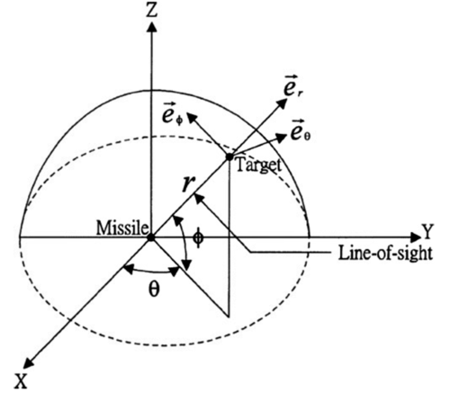
The kinematic model of the guidance system is explained in this section. The missile and target are usually considered as point masses and kinematic equations of the engagement between missile and target are written in the line of sight (LOS) coordinate frame. The center of LOS coordination is assumed as the center of mass of the missile. Figure 1 illustrates the missile and target engagement in the LOS coordination.
The missile and target engagement in the LOS coordination(Reference Shafiei and Binazadeh10).

The guidance equations in its continuous-time form are as follows(Reference Shafiei and Binazadeh10):
 \begin{align}
\dot V_\theta &= - \frac{{{V_r}{V_\theta }}}{r} + \frac{{{V_\theta }{V_\phi }\tan \phi }}{r} - {u_\theta } + {w_\theta }\nonumber\\
\dot V_\phi &= - \frac{{{V_r}{V_\phi }}}{r} - \frac{{V_\theta ^2\tan \phi }}{r} - {u_\phi } + {w_\phi }\nonumber\\
\dot \theta &= \frac{{{V_\theta }}}{{r\cos \phi }}\nonumber\\
\dot \phi &= \frac{{{V_\phi }}}{r}\nonumber\\
\dot r &= {V_r}\nonumber\\
{\dot V}_r &= \frac{{V_\theta ^2 + V_\phi ^2}}{r} - {u_r} + {w_r}
\end{align}
where  $r,\;\phi $
, and
 $\theta $
are, respectively, the relative distance between the missile and target, and yaw and pitch angles in the LOS coordination. Also, the velocity vector
 $V$
(the relative velocity between the missile and target) is defined as,
 \begin{equation*}V = [ {{V_r},{V_\theta },{V_\phi }} ] = [ {\dot r,r\dot \theta \cos \phi ,r\dot \phi } ]\end{equation*}
where  ${V_r},$
 ${V_\theta },$
and
 ${V_\phi }$
are the elements of the vector
 $\;V$
in the LOS reference frame and
 $w = {( {{w_r},{w_\theta },{w_\phi }} )^T}$
,
 $u = {( {{u_r},{u_\theta },{u_\phi }} )^T}$
are, respectively, the vectors of the missile and target. The acceleration of the missile is the input vector and the target’s acceleration is assumed as a disturbance vector. Moreover, assume that the state vector is as
 $x = [ {{V_\theta },{V_\phi },\theta ,\phi ,r,{V_r}} ]$
.
In the guidance problem, it is usually assumed that at the starting moment,  $\displaylines{
{V_r}(0) < 0, \cr
r(0) > 0 \cr} $
. This means that the missile is in the back of the target and is approaching it.
Discretisation of the guidance equations
For this purpose, Equation (6) is discretised using the first-order Euler approximation. Therefore, the guidance equations in the discrete-time form are as follow:
 \begin{equation}\left\{\begin{array}{l} {V_\theta }( {k + 1} ) = T\left( { - \dfrac{{{V_r}( k ){V_\theta }( k )}}{{r( k )}} + \dfrac{{{V_\theta }( k ){V_\phi }( k )\tan ( {\phi ( k )} )}}{{r( k )}} - {u_\theta }( k ) + {w_\theta }( k )} \right) + {V_\theta }( k )\\[10pt] {V_\phi }( {k + 1} ) = T\left( { - \dfrac{{{V_r}( k ){V_\phi }( k )}}{{r( k )}} - \dfrac{{V_\theta ^2( k )\tan ( {\phi ( k )} )}}{{r( k )}} - {u_\phi }( k ) + {w_\phi }( k )} \right) + {V_\phi }( k )\\[10pt] \theta ( {k + 1} ) = T\left( {\dfrac{{{V_\theta }( k )}}{{r( k )\cos ( {\phi ( k )} )}}} \right) + \theta ( k )\\[10pt] \phi ( {k + 1} ) = T\dfrac{{{V_\phi }( k )}}{{r( k )}} + \phi ( k ) \\[10pt] r( {k + 1} ) = T{V_r}( k ) + r( k )\\[10pt] {V_r}( {k + 1} ) = T\left( {\dfrac{{V_\theta ^2( k ) + V_\phi ^2( k )}}{{r( k )}} - {u_r}( k ) + {w_r}( k )} \right) + {V_r}( k )\end{array}\right. \end{equation}
where  $T$
is the sampling time of discretisation.
4.0 GUIDANCE LAW DESIGN
In guidance problems, it is usually tried to converge the rates of LOS rotation ( ${V_\theta }$
and
 ${V_\phi }$
) to zero or to make it as small as possible. Therefore, the discrete-time Lyapunov function
 $V$
is selected as,
 \begin{equation}V( {{x_1}} ) = V_\theta ^2(k) + V_\phi ^2(k)\end{equation}
This means that the state variables  ${x_1}$
(which asymptotic stability is desired for them) include
 ${V_\theta }$
,
 ${V_\phi }$
and the other state variables are considered as
 ${x_2}$
.
It is easy to show that the chosen Lyapunov function satisfies the conditions (2), (3) of Theorem 1.
4.1 Nominal guidance law design
First, consider the case of  $w = 0$
for Equation (7) (nominal system). The following theorem proposes a control law to stabilise the nominal system:
Theorem 2 Consider the nonlinear dynamical system (7) with  $w = 0$
and the sampling time,
 $T$
where
 $0 < T < 2$
. The following control laws
 ${u_\theta }$
,
 ${u_\phi }$
stabilise the closed-loop system asymptotically with respect to the state variables
 ${V_\theta }$
,
 ${V_\phi }$
:
 \begin{equation}\left\{ {\begin{array}{l}{{u_\theta } = - \dfrac{{{V_r}(k){V_\theta }(k)}}{{r(k)}} + \dfrac{{{V_\theta }(k){V_\phi }(k)\tan ( {\phi (k)} )}}{{r(k)}} + {V_\theta }(k)}\\[10pt] {{u_\phi } = - \dfrac{{{V_r}(k){V_\phi }(k)}}{{r(k)}} - \dfrac{{V_\theta ^2(k)\tan ( {\phi (k)} )}}{{r(k)}} + {V_\phi }(k)\;\;\;\;\;\;\;\;}\end{array}} \right.\end{equation}
Proof In the case of the nominal system,  ${\rm{\Delta }}V$
is as follows:
 \begin{align}{\rm{\Delta }}V &= {\left[ {T\left( { - \frac{{{V_r}(k){V_\theta }(k)}}{{r(k)}} + \frac{{{V_\theta }(k){V_\phi }(k)\tan ( {\phi (k)} )}}{{r(k)}} - {u_\theta }(k)} \right) + {V_\theta }(k)} \right]^2}\nonumber\\ &\quad+ {\left[ {T\left( { - \frac{{{V_r}(k){V_\phi }(k)}}{{r(k)}} - \frac{{V_\theta ^2(k)\tan ( {\phi (k)} )}}{{r(k)}} - {u_\phi }(k)} \right) + {V_\phi }(k)} \right]^2} - V_\theta ^2(k) - V_\phi ^2(k)\end{align}
If the proposed control laws (9) are inserted in (10),  $\Delta V$
of the closed-loop system will be as,
 \begin{equation}{\rm{\Delta }}V = ( {{T^2} - 2T} )( {V_\theta ^2(k) + V_\phi ^2(k)} )\end{equation}
Since for the sampling time we have  $0 < T < 2$
, thus,
 \begin{equation*}{\rm{\Delta }}V \le - \beta (\| {V_\theta ^2(k)\| + \|V_\phi ^2(k)}\| )\end{equation*}
where  $0 < \beta < {T^2} - 2T$
. Therefore, the condition (4) is satisfied and according to Theorem 1, the asymptotical stability of the nominal closed-loop system is guaranteed.□
4.2 Design of the discrete-time robust guidance law
In the following theorem, the designed discrete-time guidance law is made robust using the Lyapunov redesign method.
Theorem 3: Consider the nonlinear dynamical system (7) with  $w \ne 0$
and the sampling time, T where
 $0 < T < 2$
. The following control laws
 ${u_\theta }$
,
 ${u_\phi }$
lead to the ultimate boundedness of the state variables
 ${V_\theta }$
,
 ${V_\phi }$
in the closed-loop system:
 \begin{equation}\left\{ {\begin{array}{c}{{u_\theta } = - \dfrac{{{V_r}(k){V_\theta }(k)}}{{r(k)}} + \dfrac{{{V_\theta }(k){V_\phi }(k)\tan ( {\phi (k)} )}}{{r(k)}} + {V_\theta }(k) + K{\rm{sgn}}( {{V_\theta }(k)} )}\\[10pt] {{u_\phi } = - \dfrac{{{V_r}(k){V_\phi }(k)}}{{r(k)}} - \dfrac{{V_\theta ^2(k)\tan ( {\phi (k)} )}}{{r(k)}} + {V_\phi }(k) + K{\rm{sgn}}( {{V_\phi }(k)} )\;\;\;\;\;\;\;\;}\end{array}} \right.\end{equation}
where
 \begin{equation}K = \frac{{\eta ( {2 + 2{T^2} - 5T} )}}{{( {2 - T} )}} + \frac{{\eta \sqrt {16 - 48T + 52{T^2} - 24{T^3} + 4{T^4}} }}{{( {2 - T} )}}\end{equation}
and  $\eta $
is an upper bound for all the elements of the vector w.
Proof For the case of manoeuvering targets (when  $w \ne 0$
), the term
 ${\rm{\Delta }}V$
will be as follows:
 \begin{align}{\rm{\Delta }}V &= {\left[ {T\left(\! { - \frac{{{V_r}(k){V_\theta }(k)}}{{r(k)}} + \frac{{{V_\theta }(k){V_\phi }(k)\tan ( {\phi (k)} )}}{{r(k)}} - {u_\theta }(k) + {w_\theta }(k)} \!\right) + {V_\theta }(k)} \right]^2}\!\!- V_\theta ^2(k)\nonumber\\[6pt] &\quad+ {\left[ {T\left( { - \frac{{{V_r}(k){V_\phi }(k)}}{{r(k)}} - \frac{{V_\theta ^2(k)\tan ( {\phi (k)} )}}{{r(k)}} - {u_\phi }(k) + {w_\phi }(k)} \right) + {V_\phi }(k)} \right]^2} - V_\phi ^2(k)\end{align}
If the control laws are selected as
 \begin{equation}\left\{ {\begin{array}{c}{{u_{\theta new}} = {u_\theta }(k) + {v_1}(k) = - \dfrac{{{V_r}(k){V_\theta }(k)}}{{r(k)}} + \dfrac{{{V_\theta }(k){V_\phi }(k)\tan ( {\phi (k)} )}}{{r(k)}} + {V_\theta }(k) + {v_1}(k)}\\[10pt] {{u_{\phi new}} = {u_\phi }(k) + {v_2}(k) = - \dfrac{{{V_r}(k){V_\phi }(k)}}{{r(k)}} - \dfrac{{V_\theta ^2(k)\tan ( {\phi (k)} )}}{{r(k)}} + {V_\phi }(k) + {v_2}(k)\;\;\;\;\;\;\;\;}\end{array}} \right.\end{equation}
Then, substituting Equation (15) in (14) leads to
 \begin{align}{{\Delta }}V &= ( {{T^2} - 2T} )V_\theta ^2( k ) + \left[ {T^2}{{( {{v_1}( k )} )}^2} - 2{T^2}{w_\theta }( k ){v_1}( k ) - 2{T^2}{w_\theta }( k ){V_\theta }( k )\right.\nonumber\\[4pt] &\quad+ \left.2T{w_\theta }( k ){V_\theta }( k ) + {T^2}{{( {{w_\theta }( k )} )}^2} + 2{T^2}{V_\theta }( k ){v_1}( k ) - 2T{V_\theta }( k ){v_1}( k ) \right] + ( {{T^2} - 2T} )V_\phi ^2( k )\nonumber\\[4pt] &\quad+ \left[ {T^2}{{( {{v_2}( k )} )}^2} - 2{T^2}{w_\phi }( k ){v_2}( k ) - 2{T^2}{w_\phi }( k ){V_\phi }( k ) + 2T{w_\phi }( k ){V_\phi }( k ) + {T^2}{{( {{w_\phi }( k )} )}^2}\right.\nonumber\\[4pt] &\quad+ \left.2{T^2}{V_\phi }( k ){v_2}( k ) - 2T{V_\phi }( k ){v_2}( k ) \right]\end{align}
In (16), the instantaneous values of the variables  ${w_\theta }$
,
 ${w_\phi }$
are unknown and only an upper bound for them is given, i.e.
 \begin{equation*}\|{w_\theta }\| < \eta ,\; \|{w_\phi }\| < \eta ,\; \|{w_r}\| < \eta \end{equation*}
Therefore, by assuming  ${v_1}(k) = K{\rm{sgn}}( {{V_\theta }(k)} )$
,
 ${v_2}(k) = K{\rm{sgn}}( {{V_\phi }(k)} )$
where
 $K > 0,$
we have
 \begin{align}{\rm{\Delta }}V &\le ( {{T^2} - 2T} )V_\theta ^2(k) + \left[ {T^2}{K^2} + 2{T^2}\eta \left| K \right| + 2T\eta \left| {{V_\theta }(k)} \right|\left( {T + 1} \right) + {T^2}{\eta ^2}\right.\nonumber\\[4pt]
&\quad+ \left. 2TK\left( {T - 1} \right)\left| {{V_\theta }(k)} \right| \right] + ( {{T^2} - 2T} )V_\phi ^2(k) + \left[ {T^2}{K^2} + 2{T^2}\eta \left| K \right|\right.\nonumber\\[4pt]
&\quad+ \left. 2T\eta \left| {{V_\phi }(k)} \right|\left( {T + 1} \right) + {T^2}{\eta ^2} + 2TK\left( {T - 1} \right)\left| {{V_\phi }(k)} \right| \right]\end{align}
As can be seen, Equation (17) contains two quadratic equations with respect to  $\left| {{V_\theta }(k)} \right|$
and
 $\left| {{V_\phi }(k)} \right|$
. If
 $K$
is chosen such that both of these equations become negative, the term
 ${\rm{\Delta }}V$
is always negative, too. Coefficients of these two quadratic equations are as follow:
 \begin{align*}a &= ( {{T^2} - 2T} ) < 0 \\ b &= 2TK\left( {T - 1} \right) + 2T\eta \left( {T + 1} \right)\\c &= {T^2}{K^2} + {T^2}{\eta ^2} + 2{T^2}\eta K \end{align*}
In these equations,  $a < 0$
and
 \begin{equation*}\Delta' = 4{T^3}\eta \left( {\eta + K} \right) + {T^2}{\left( {\eta - K} \right)^2} > 0\end{equation*}
Moreover, the product of the roots of each of these equations (which is equal to c/a ${\raise0.7ex\hbox{$c$} \!\mathord{\left/
{\vphantom {c a}}\right.}
\!\lower0.7ex\hbox{$a$}}$
) is negative. Therefore, these equations have real roots with different signs. Since the equations are in terms of absolute values of
 ${V_\theta }(k)$
and
 ${V_\phi }(k)$
, only the positive root is admissible.
Now it is proved that the asymptotical stability of the closed-loop system is not possible. By the principle of contradiction, suppose that  ${\rm{\Delta }}V$
is always negative for any values of
 ${V_\theta }(k)$
and
 ${V_\phi }(k)$
. This means that the variables
 ${V_\theta }(k)$
and
 ${V_\phi }(k)$
converge to zero as
 $k \to \infty $
. However, it can be seen that if
 ${V_\theta }(k)$
and
 ${V_\phi }(k)$
converge toward zero, the following result is obtained according to (10):
 \begin{equation}{\rm{\Delta }}V = {T^2}{\left( {{v_1} - {w_\theta }} \right)^2} + {T^2}{\left( {{v_2} - {w_\phi }} \right)^2}\end{equation}
That is always non-negative. Thus, it is not possible to have a negative definite  ${\rm{\Delta }}V$
. Therefore, in this paper, the ultimate boundedness of the variables
 ${V_\theta }(k)$
and
 ${V_\phi }(k)$
will be proved and it is tried to make them as small as possible.
The roots of the equations in (17) are as follow:
 \begin{equation}\left| {{V_\theta }(k)} \right| = \frac{{ - b' \pm \sqrt {\Delta'} }}{a} = - \frac{{\left[ {T\left( {\eta + K} \right) + \left( {\eta - K} \right)} \right]}}{{T - 2}} \pm \frac{{\sqrt {{{\left( {\eta - K} \right)}^2} + 4T\eta \left( {\eta + K} \right)} }}{{T - 2}}\end{equation}
Thus, according to the sign of the coefficients of quadratic equations, if  $\left| {{V_\theta }(k)} \right|$
is greater than the positive root (larger root), the term
 ${\rm{\Delta }}V$
will be negative. In order to minimise the upper limit of
 $\left| {{V_\theta }(k)} \right|$
, the positive root can be minimised using the parameter
 $K$
. For the variable
 $\left| {{V_\theta }(k)} \right|$
, it is the case, too. To find the value of
 $K$
which minimises the positive root, using basic calculus one has
 \begin{equation}\frac{\partial }{{\partial K}}\left( {\frac{{\left[ {\eta \left( {T + 1} \right) + K\left( {T - 1} \right)} \right]}}{{2 - T}} + \frac{{\sqrt {{{\left( {\eta - K} \right)}^2} + 4T\eta \left( {\eta + K} \right)} }}{{2 - T}}} \right)=0\end{equation}
After differentiation and simplification, a new quadratic equation with respect to K will be obtained as follows:
 \begin{equation}( {{T^2} - 2T} ){K^2} + \left( {4T\eta + {4^3}\eta - 10{T^2}\eta } \right)K + 4{T^3}{\eta ^2} - 11{T^2}{\eta ^2} + 2T{\eta ^2} = 0\end{equation}
Finally, according to the assumption of  $K > 0$
, the admissible value of K is calculated as follows:
 \begin{equation}K = \frac{{\eta ( {2 + 2{T^2} - 5T} )}}{{2 - T}} + \frac{{\eta \sqrt {16 - 48T + 52{T^2} - 24{T^3} + 4{T^4}} }}{{2 - T}}\end{equation}
Now, the value of  $K$
can be evaluated and replaced in Equation (19) to find the positive root of the quadratic Equation in (17). If the value of this positive root is called
 $\alpha $
, then according to the above discussion, the amount of
 ${\rm{\Delta }}V$
will be negative for
 $\left| {{V_\theta }(k)} \right| > \alpha $
and thus
 $\left| {{V_\theta }(k)} \right|$
will be ultimately bounded in the range of
 $\left[ { - \alpha , + \alpha } \right]$
.
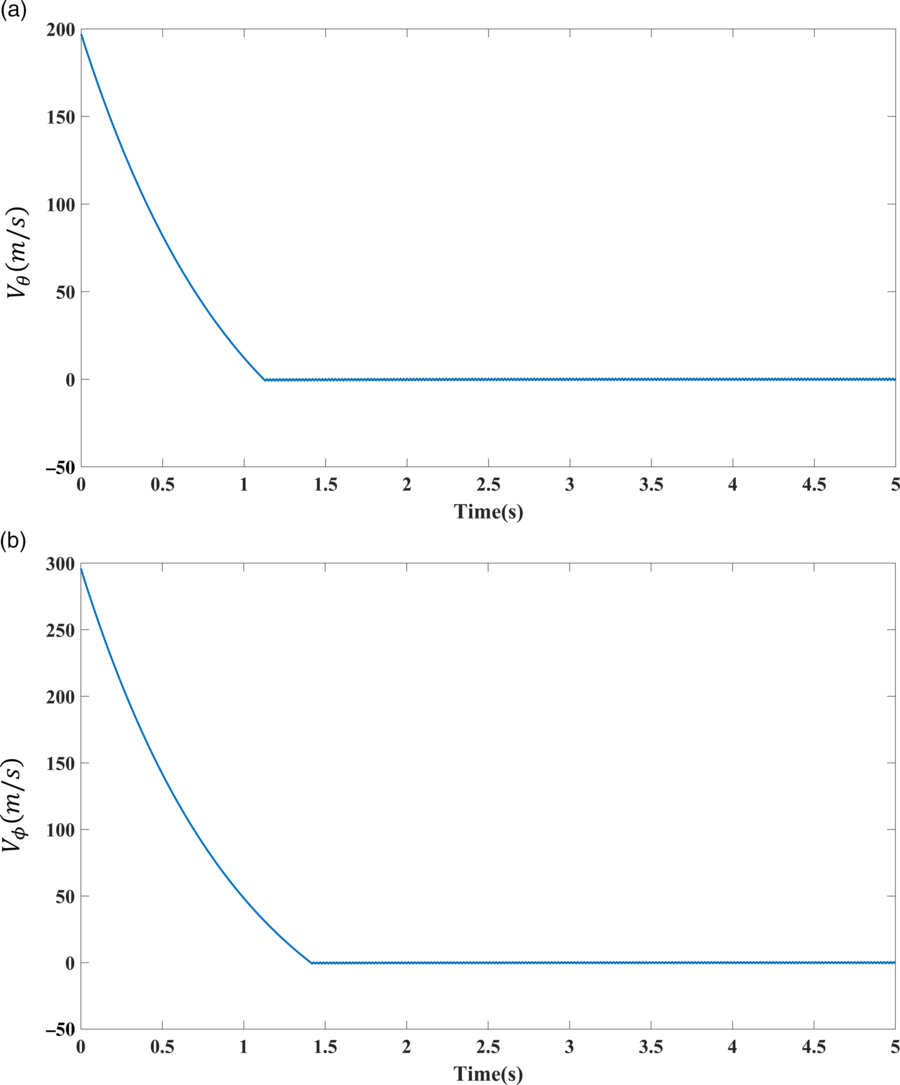
The convergence of (a)  ${\textit{V}_\theta }\text{(}\textit{k}\text{)}$
and (b)
 ${\textit{V}_\phi }\text{(}\textit{k}\text{)}$
, in the case of a non-manoeuvering target.

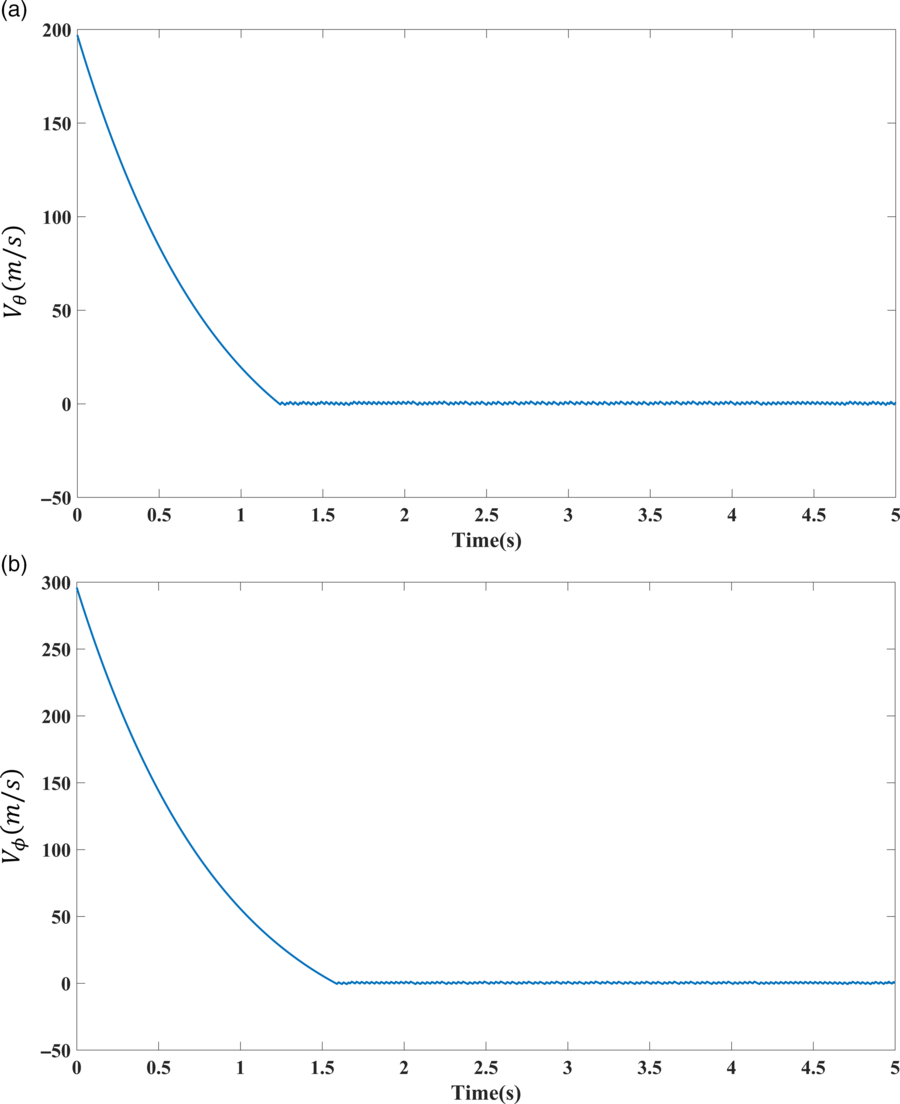
The convergence of (a)  ${\textit{V}_\theta }\text{(}\textit{k}\text{)}$
and (b)
 ${\textit{V}_\phi }\text{(}\textit{k}\text{)}$
, to zero in the case of a manoeuvering target.

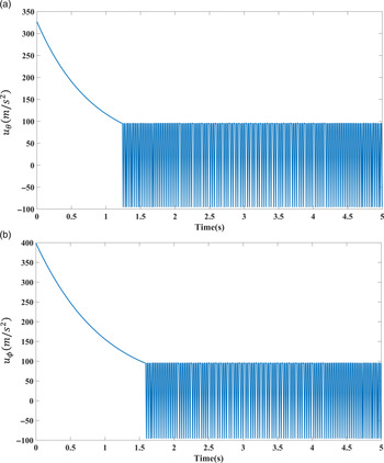
The control signals (a)  ${\textit{u}_\theta }$
and (b)
 ${\textit{u}_\phi }$
in the presence of a manoeuvering target.

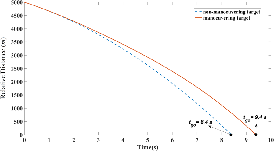
The relative distance between the missile and target.

4.3 Investigation of the collision
The collision occurs when the relative distance between the missile and target permanently decreases and finally becomes zero ( $r = 0$
), at a moment. In this engagement, the missile’s approaching rate to the target (
 ${V_r}(k)$
) is guaranteed to be negative using the following proposed controller:
 \begin{equation}{u_r}(k) = \frac{{V_\theta ^2(k) + V_\phi ^2(k)}}{{r(k)}} + \eta \end{equation}
If the control law  ${u_r}(k)$
is substituted in the equation of
 ${V_r}( {k + 1})$
in (7), the following equation will be achieved:
 \begin{equation*}{V_r}( {k + 1}) = T( { - \eta + {w_r}(k)} ) + {V_r}(k)\end{equation*}
Since  ${w_r}(k) < \eta $
, then
 ${V_r}( {k + 1})$
will be negative with considering this fact that the initial condition of
 ${V_r}( . )$
has been assumed negative. The problem is only the singularity of the fractional term around
 $r = 0$
. Since the converging rate of the variables
 ${V_\theta }(k)$
and
 ${V_\phi }(k)$
is more than
 $r(k)$
, therefore, the nominator will converge to zero before the denominator and consequently, the control signal would not be unbounded before the collision. In many of missiles, a complicated time-varying trust force is un-implementable. If in the worst-case scenario
 $\sup_k \left( {\frac{{V_\theta ^2(k) + V_\phi ^2(k)}}{{r(k)}}} \right) + \eta $
is evaluated through simulation, the trust acceleration should be chosen to be greater than this constant value.
5.0 SIMULATION RESULTS
In this section, the performance of the proposed guidance law is evaluated through simulations. In the simulations, first, a target without manoeuvering is considered. Then, the guidance loop is simulated with considering a manoeuvering target with sinusoidal accelerations in all directions as  ${w_{r,\theta ,\phi }} = 40\sin ( {0.5{\rm{t}}} )$
. In both cases, the initial values have been selected as,
 ${r_0} = 5{\rm{km}}$
,
 ${\theta _0},{\phi _0} = \pi /3$
,
 ${V_r}(0) = - 300{\rm{m}}/{\rm{s}}$
,
 ${V_\theta }(0) = 200{\rm{m}}/{\rm{s}}$
,
 ${V_\phi }(0) = 300{\rm{m}}/{\rm{s}}$
,
 $T = 0.01$
.
In the case of the non-manoeuvering target (i.e. in the absence of disturbances), the convergence of the state variables to zero is demonstrated in Fig. 2.
As seen in Fig. 2, the components of the rotation of the LOS vector have converged to a small bound around zero. Figures 3 and 4 show the state variables of the system (rotation rates of the LOS vector) and the resulting control laws in the presence of disturbances, respectively.
In this case, it is observed that the state variables of the system are ultimately bounded to a small interval. This interval is related to the chosen Lyapunov function and the sampling time, T. Although the state variables have not been converged exactly to zero, the collision of the missile and target is guaranteed in a finite time (Fig. 5), using the proposed controller.
In Fig. 4 the amplitude of control signals in  $\theta ,\phi $
directions has been shown. This figure shows that the maximum amplitude of these lateral accelerations between 30g and 40g, which can be implemented in the ground-to-air missiles. Figure 5 shows the relative distance between the missile and the target for both cases (manoeuvering and non-manoeuvering targets). Crossing the relative distance from zero value shows that the collision has occurred.
6.0 CONCLUSIONS
In this paper, the approach of discrete-time partial stabilisation was used to design a robust three-dimensional guidance law. The main problem of the existing guidance laws that are based on continuous-time partial stabilisation is that their implementation is usually using digital systems and transforming a continuous-time guidance law to discrete-time form may produce inefficiencies or even instability. On the other hand, in other discrete-time guidance laws, the theory of partial stabilisation had not been used. As was discussed in this paper, this theory is more compatible with the physical properties of the guidance problem. Moreover, in contrast to many papers considering a two-dimensional case, in this paper, a three-dimensional guidance problem was considered. On the other side, it was shown in the theoretical and simulation sections that the proposed guidance law is robust against the manoeuverings of the target and the ultimate boundedness of the state variables was guaranteed. Then, based on the analysis of second-order equations, the ultimate error band of the state variables was minimised as possible. Finally, to guarantee the collision of the missile to the target, a proper longitudinal acceleration was designed for the missile. Simulation results showed the appropriate performance of this guidance law in the case of nominal and manoeuvering targets.