



Nomenclature
- AR
-
area ratio
- BP
-
blade passing frequency [Hz]
- C
-
chord length [mm]
- CFD
-
computational fluid dynamics
- CP
-
choke point
-
 $C_{p}$
-
coefficient of pressure
-
$C_{t}$
-
rotor tip chord [mm]
- CV
-
corner vortex
- CWT
-
continuous wavelet transformation
- F
-
frequency [Hz]
- FFT
-
fast Fourier transformation
- h
-
duct height [mm]
- HP
-
high pressure
- IGV
-
inlet guide vane
- ISD
-
inter-stage duct
- L
-
duct length
- LP
-
low pressure
- M
-
mach number
- m
-
mass flow rate [kg/s]
- N
-
rotational speed[RPM]
- NS
-
near stall
- NSF
-
near stall flow
- OGV
-
outlet guide vane
- P
-
pressure [Pa]
- PE
-
peak efficiency
- PR
-
pressure ratio
- S
-
entropy [J/kg.K]
- R
-
radius [mm]
- RANS
-
Reynolds averaged Navier–Stokes
- T
-
time [s]
- t
-
time step


Greek symbol
-
$\eta$
-
efficiency
-
$\Delta$
-
interval
-
$\omega$
-
vorticity vector


1.0 Introduction
The increasing environmental concerns have made a paradigm shift in gas-turbine engines with respect to achieving a high thrust-to-weight ratio, low emissions, reduced noise and high bypass ratios in turbofan engines. The technological advancements in core turbomachinery components are reaching a threshold, making even an incremental improvement quite hard. This has drawn attention to the other non-rotating components, such as the inter-spool duct (ISD), being used in turbofan engines. This duct serves as a connecting passage between low-pressure (LP) and high-pressure (HP) spools in the compressor and turbine sections. The inter-spool duct usually has an S-shape profile dictated by the engine architecture and huge area change across the LP and HP spools. A well-designed ISD has the potential to offer better weight savings, reduction in aerodynamic losses and noise levels by ensuring a continuous mass flow rate with low turbulence levels across the spools. However, the design space of the ISD is very narrow due to the dependency on flow quality from the upstream component and the high radius of curvature, which makes it very susceptible to boundary layer separation from the end walls at off-design operating points. Therefore, a state-of-the-art ISD design needs an integrated approach accounting for the flow quality from upstream components and its critical geometrical features. Many researchers have made extensive efforts to explore the aerodynamics of compressor inter-spool ducts, enabling the understanding of flow patterns, pressure losses, and efficiency implications. This will eventually help broaden the design space for ISD design. This can be seen in the work available in the literature. Bailey et al. [Reference Bailey, Britchford, Carrote and Stevens1] investigated a compressor duct with and without the upstream compressor and reported that the curvature of the duct plays an important role in setting up a streamwise adverse pressure gradient. This also affects turbulence generation and flow separation. The duct with upstream compressors incurs more total pressure loss due to high turbulent mixing. Britchford et al. [Reference Britchford, Carrotte, Kim and Hield2] applied a row of tangentially leaned outlet guide vanes (OGVs) in the first bend of a compressor duct to reduce the loading on the duct’s inner wall and achieved a significant reduction in flow separation. Karakasis et al. [Reference Karakasis, Naylor, Miller and Hodson3] studied a duct with axisymmetric and non-axisymmetric endwalls with upstream and downstream LP compressor stages. They observed that the maximum duct losses are caused by the upstream stator wakes, particularly on the duct hub wall. Ortiz et al. [Reference Ortiz Duenas, Miller, Hodson and Longey4] investigated the effect of length reduction in the compressor duct using experimental and numerical approaches, followed by optimisation to reduce the total pressure loss. They found that, with reducing length, the losses increased due to the early separation of the boundary layer. Also, the size of the separation was strongly dependent on the Reynolds number.
Naylor et al. [Reference Naylor, Dueñas, Miller and Hodson5] designed a more aggressive compressor duct with struts and non-axisymmetric endwall profiling to reduce losses. Their study demonstrated a 16% reduction in overall losses. Walker et al. [Reference Walker, Barker and Carrotte6] numerically and experimentally evaluated a novel concept of bleed in the compressor duct separation area. The study showed a reduction of 20% in duct loss by delaying the separation with a 30% smaller length of the overall system than the conventional one. In a subsequent study, Walker et al. [Reference Walker, Barker, Carrotte, Bolger and Green7] introduced OGV in the first bend of the duct. These OGVs were provided with lean and sweep 3D features to balance the radial pressure fields. Using the OGVs in the duct helped to reduce the system length by 21%, and the balancing of the pressure fields helped to keep the upstream rotor performance unaffected. Also, the overall losses were unaffected by a more uniform exit flow. Sturzebecher et al. [Reference Sturzebecher, Goinis, Voss, Sahota, Groth and Hammer8] carried out optimisation studies for an already aggressive duct fitted with OGVs in two stages. First, the duct was optimised for length reduction, and then the wall contouring was done with strut blade parameterisation to avoid corner separation. The study showed that corner separation can be avoided with minimal possible losses.
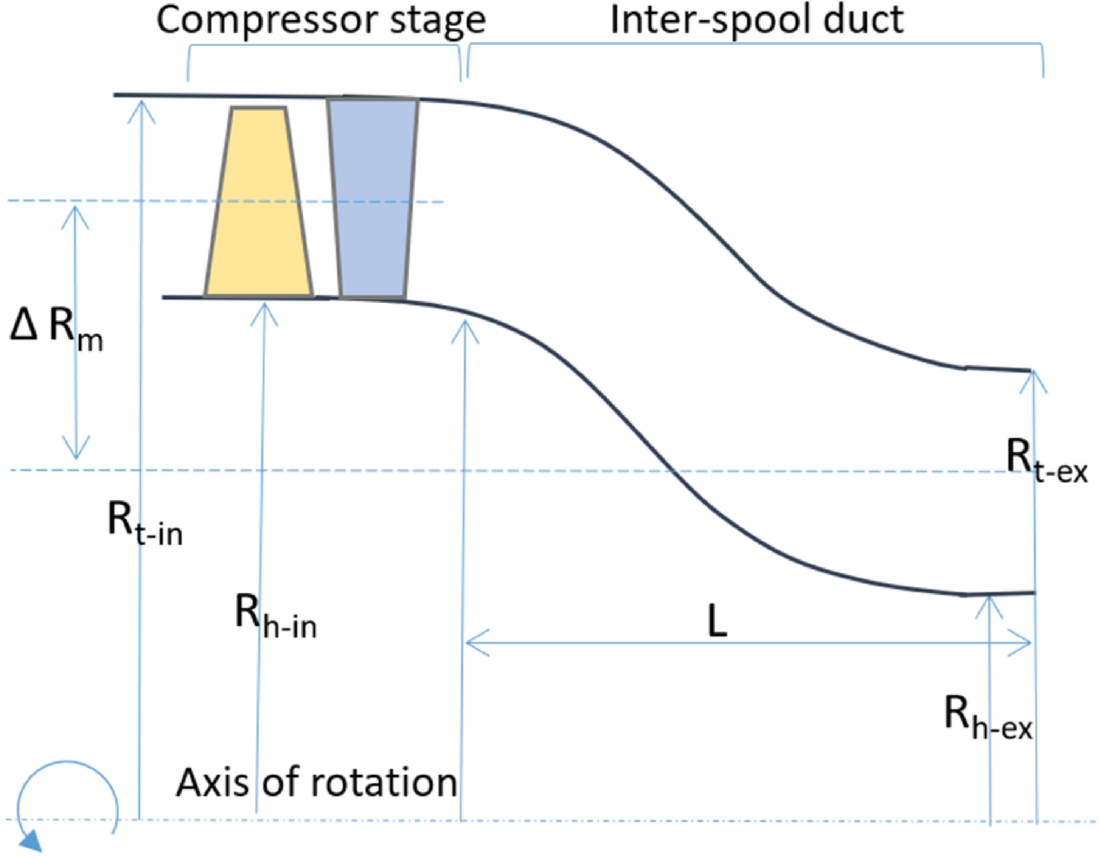
Verma et al. [Reference Verma, Singh and Pradeep9] explored the flow interaction in a turbofan system having an upstream fan, ISD and downstream booster stage. They also applied shape optimisation of the ISD for performance improvement. They reported that there is a significant difference in the independent duct performance from that in the integrated system due to strong coupling with the upstream stator secondary flow structures. In the next study, Verma et al. [Reference Verma, Singh and Pradeep10] studied the effect of distortion on the same system by applying the stepped total pressure profile in the hub and tip region at the inlet. They observed that with the smaller levels, hub distortion helps improve the stall margin, and tip distortion does the opposite. However, with increasing levels, the hub distortion causes a rapid reduction in the stall margin compared to the tip one. Walker et al. [Reference Walker, Mariah, Tsakmakidou, Vadhvana and Hall11] investigated the effect of fan root flow on the engine section splitter and compressor duct using experimental and computational techniques with a 1.5 compressor stage. The study reported that the root flow has a significant role in downstream component loss generation. Xin et al. [Reference Xin, Zhao, Tian, Kong and Lu12] performed an experimental study for a strutted compressor duct and analysed the effect of varying inlet conditions on the duct aerodynamics. The duct profile modification near the duct helped to reduce the loss and eliminate the corner separation. Fritz et al. [Reference Fritz, Dygutsch, Kasper, Hergt, Grund, Flamm, Lejon and Sahota13] conducted an experimental study on a non-rotating test rig to simulate the effect of upstream swirler disturbances and a downstream inlet guide vane (IGV) with an inter-compressor duct. The study concluded with detailed insight into the secondary flow system in the duct. Sharma et al. [Reference Sharma and Baloni14] studied the effect of stream-wise adverse pressure gradient and wall curvature on duct flow physics. It was reported that the upper wall operates under a favourable pressure gradient. In contrast, the lower wall is subjected to an adverse pressure gradient, causing flow separation. A similar design philosophy is attempted in the present study. A compressor ISD design is carried out using cubic Bezier curves matching the exit annulus of an existing tip-critical transonic axial compressor stage. A graphical representation of this system is illustrated in Figure 1.
This study aims to analyse the aerodynamic interactions between ISD and the upstream compressor stage in terms of performance parameters such as pressure ratio, efficiency, stall characteristics and flow diagnostics of both components at design and off-design operating conditions through numerical simulations. Particularly, the emphasis is placed on understanding the effect of compressor flow features in ISD flow physics. The unsteady computational fluid dynamic (CFD) simulations are carried out to analyse the response of the integrated system at the near-stall condition and analyse the secondary flow system in the duct. The results are presented with the help of performance maps, flow contours, Q criterion and fast Fourier transformation (FFT) of the unsteady pressure signals at various points in the system.
2.0 Geometrical details
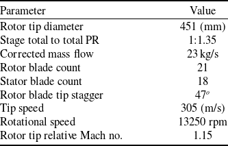
The geometrical setup consists of an upstream transonic compressor stage and a downstream inter-spool duct. The compressor stage is a research compressor in the Propulsion Division, National Aerospace Laboratories, and its technical specifications are available in Table 1 [Reference Kumar, Alone and Pradeep15]. The ISD is designed using a cubic Bezier curve having four control points given by equations 1 and 2. The inlet annulus height of the duct is derived from the compressor stage exit boundary. The duct flow path has an inner wall profile and an outer wall profile.
Technical specifications of the transonic axial flow compressor stage

Table 1. Long description
A table with 8 rows and 2 columns. The first column lists parameters and the second column lists their corresponding values. Row 1: Parameter, Value. Row 2: Rotor tip diameter, 451 millimeters. Row 3: Stage total to total PR, 1:1.35. Row 4: Corrected mass flow, 23 kilograms per second. Row 5: Rotor blade count, 21. Row 6: Stator blade count, 18. Row 7: Tip speed, 305 meters per second. Row 8: Rotational speed, 13250 revolutions per minute. Row 9: Rotor tip relative Mach number, 1.15.
Graphical representation of the compressor stage and ISD.

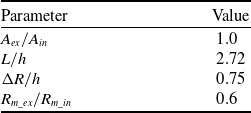
The geometric details of the ISD are given in Table 2. The duct inlet height is 92 mm. The duct area ratio (
 $\frac {A_{ex}}{A_{in}}$
) at the inlet and exit is constant, as can be seen from the area distribution in Figure 2. The duct length (
 $L$
) and the other derived quantities mentioned in the table are chosen based on the guidelines given in Reference [Reference Bailey, Britchford, Carrote and Stevens1]. Also, an extension of five times the ISD exit height was added after plane 4. This was essential to ensure that the flow structures occurred in the duct had enough space to move out of the ISD domain, and there should not be any reverse flow and boundary reflection effects.
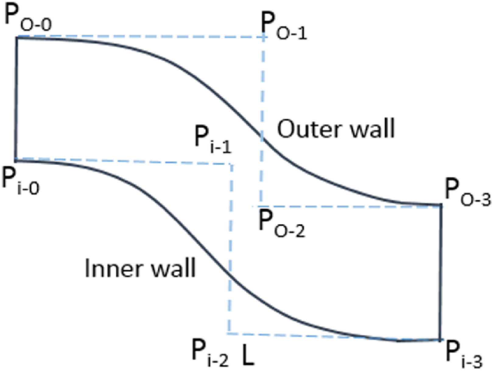
There are a total of eight control points in the ISD flow path, out of which the end control points at the inlet and exit are fixed, and the four points in the middle define the shape of the duct, as shown in Figure 3. The
 $P_{o-j}$
and
 $P_{i-j}$
represent the control points at the outer and inner wall profiles. The designed duct has a constant area throughout.
 \begin{equation} B(t)=\sum _{i=o}^{n}P_{i} b_{i,n} \end{equation}
 \begin{equation} b_{i,n}(t)=\frac {n!}{n!(n-1)!}t^{i}(1-t)^{n-1} \end{equation}
Geometrical details of the ISD

Table 2. Long description
A table with two columns and five rows. The first column is labeled Parameter and the second column is labeled Value. Row 1: Parameter, A subscript ex over A subscript in; Value, 1.0. Row 2: Parameter, L over h; Value, 2.72. Row 3: Parameter, Delta R over h; Value, 0.75. Row 4: Parameter, R subscript m, ex over R subscript m, in; Value, 0.6.
ISD area ratio variation over the length.

Duct inner and outer wall profiles with control points.

Here,
 $t$
is a dimensionless length and varies between 0 and 1.
 $P_{i}$
is function of coordinates.
 $b_{i}$
,
 $n(t)$
is the Bernstein basis function, and
 $n$
shows the order of the Bezier curve.
3.0 Numerical setup details
A 3D one-blade row model is adopted for computational analysis, where one blade of the rotor passage and one blade of the stator passage are considered with a pitch ratio of 0.86. The ISD is taken as
 $20^{o}$
sector having a pitch ratio of 1 with the stator passage. The computational domain is shown in Figure 4.
3D computational domain.

Planes 1, 2, 3 and 4 are the measurement planes. The red circular dots represent the unsteady numerical probes. The instantaneous static pressure signals are recorded with the help of these probes to analyse the unsteady response of the compressor stage and ISD. The stage inlet boundary is defined as a pressure inlet. The inlet total pressure and temperature values are taken from the experimental data. The stage exit is defined as a pressure outlet having a uniform static pressure distribution. The hub and shroud surfaces are defined as no-slip walls, except the rotor shroud being a counter-rotating no-slip wall in the relative frame. The side boundaries are defined as rotational periodic walls. The interface between the rotor and stator domains is defined as a mixing plane for the Reynolds averaged Navier–Stokes (RANS) simulations. For the unsteady Reynolds averaged Navier–Stokes (U-RANS), a transient blade row model is used with profile transformation at the interface. A tip clearance of 0.6 mm was given for the rotor, whereas the stator has no clearance.
The steady and unsteady RANS simulations are performed using ANSYS-CFX. The second-order high-resolution scheme with an auto time scale is chosen for steady RANS. Meanwhile, for U-RANS, a second-order backward Euler scheme is chosen. The unsteady simulations are carried out for ten rotor revolutions. One stator pitch passing of the rotor blade is divided into 20 time steps, having ten internal coefficients of loop iterations. The resultant time step size is
 $1.19\times 10^{-5}$
seconds. The shear stress transport (SST) model is used in all the simulations for the closure of the turbulence quantities [Reference Kumar, Alone and Pradeep16].
Distribution of
 $Y^{+}$
in the computational domain.

The
 $Y^{+}$
value is maintained small enough to meet the turbulence model requirements, as illustrated in Figure 5. Geometry meshing is carried out using ANSYS TurboGrid. A mixed O-H topology is used for generating a hexahedral mesh in the entire domain, as shown in Figure 6. A mesh independence test is performed using five mesh densities of various sizes (2.5, 3, 3.75, 4.5 and 5 million) for the maximum total pressure rise in the entire stage, as shown in Figure 7. The difference between 4.5 and 5 million mesh size was found to be 0.026%, which can be neglected. Therefore, the mesh size of 4.5 million was used for the entire study.
Mesh density at various locations in the domain.

Variation of max pressure rise with various mesh sizes.

4.0 Results and discussion
4.1. Compressor stage performance validation as stand-alone component
Figure 8(a) shows the stand-alone compressor stage total pressure ratio (PR) performance validation with the experimental data available at 80% and 90% of the design speed [Reference Kumar, Bhanudasji Alone, Dilipkumar, Shobhavathy, Mudipalli, Kumar, Ganguli, Kandagal and Jana17] using steady RANS simulations. Also, the rotor tip static pressure at the choke point (CP) and near-stall flow (NSF) is validated for 80% speed given in Figure 8(b). In both validation figures, the average deviation between the experimental and numerical data is under 0.15% and can be considered within the numerical uncertainty [Reference Sun, Wang, Wang, Wang and Magagnato18].
Performance characteristics validation of stand-alone compressor stage.

4.2. Integrated performance of compressor stage and ISD
Figure 9(a) and (b) show the total PR and efficiency versus corrected mass flow characteristics of the integrated system at 100% of the design speed. Here, the curve with a violet triangle shows the stand-alone compressor performance, whereas the curve with a green square box and orange diamond shape shows the stage performance in an integrated system with and without the ISD. Without a duct, the curve is plotted considering measurements at planes 1 and 3 as marked in Figure 4.
Performance characteristics of integrated system at 100% speed.

Entropy generation in the streamwise direction in the stage with and without ISD at the near-stall (NS) point.

Meanwhile, with the duct, the curve is plotted from the data taken at planes 1 and 4 (ISD exit). The operating points where data analysis is carried out are marked in the total PR graph as CP, Peak Efficiency (PE), and NS points. With the downstream duct, there is a reduction in the overall mass flow by 1.8% due to the thick boundary layer on the ISD inner and outer walls. Also, a 5.8% reduction in the choke margin is observed for the stage and integrated system; however, there is a rise in the stall mass flow limit with the ISD downstream, which is marked in Figure 9(a).
Apparently, the choke margin reduction is due to the combined effect of thick wall boundary layers in the duct and the blockage at the duct exit caused by the swirl-induced reverse flow. The stall margin improvement is essentially due to the stage instabilities getting transferred to the duct before growing in the blade passage. However, the losses occurring in the duct have reduced the overall efficiency of the integrated system by 2.0%, as can be seen in Figure 9(b).
The comparison of losses occurring in the compressor stage with and without ISD at the NS point is shown in Figure 10. Here, the horizontal axis is normalised, and the distance
 $0$
to
 $1$
shows rotor passage, while
 $1$
to
 $2$
shows stator passage. As can be seen over the distance from
 $0$
to
 $0.5$
, the entropy generation is the same in the rotor for both cases, however, it has significantly increased to a peak value
 $67.6 J/kg.K$
for the case with ISD and then drops to
 $61.8 J/kg.K$
after the flow has crossed the blade and exited the rotor passage. This is attributed to the combined effect of shock-induced flow separations and tip leakage flow in the rotor. In the case without ISD, although the mechanism of losses remains the same, the magnitude is relatively lower, which is reflected in the trend of entropy generation. The overall percentage increase in the entropy at rotor exit is around
 $11\%$
. Similarly, in the stator passage, as the flow moves across the blade, the streamwise adverse pressure gradient and the radial pressure gradient cause corner flow separation, which leads to a rise in entropy. With flow exiting the blade passage, there is a drop in entropy for both cases. However, for the case with ISD, after the drop, the entropy generation is constant up to a distance of
 $0.8$
; later, there is a steep rise in it near the exit, as marked by a circle. This sudden rise is caused by the flow separation near the exit of ISD, particularly near the stall inception. The overall entropy rise with ISD is
 $10.5\%$
.
4.3. Duct performance using steady RANS
The coefficient of static pressure (
 $C_{p}$
) variation on the wall is dictated by the wall contours (3). The
 $C_{p}$
is calculated by taking the mass-averaged value of the inlet total pressure and the area-averaged value of the static pressure at the inlet and along the wall. The static pressure rises in the duct as the compressor mass flow decreases, which can be observed from the
 $C_{p}$
distribution for CP, PE and NS given in Figure 11(a) and (b). A very small fluctuation in the
 $C_{p}$
can be seen at the ISD entry due to the local acceleration or deceleration in the stator corner separation region. As the flow enters the duct, it encounters the concave surface, causing the flow to diffuse at the upper wall and the subsequent rise in static pressure. As the flow crosses half the length of the duct, the upper wall contour tends to be convex, causing the acceleration and a subsequent decrease in static pressure. Near the duct exit, there is a sudden rise in the
 $C_{p}$
due to the local diffusion, causing the local pressure rise as can be seen in the non-dimensional static pressure contours in Figure 12(a), (b) and (c) for CP, PE and NS.
At the duct lower wall, the convex wall contour causes flow acceleration, leading to a decrease in the
 $C_{p}$
for all the operating points. However, irrespective of the wall contour, there is a drop in static pressure at the lower wall throughout the duct. This is caused by the swirl component of the flow coming out of the stator passage. This swirling flow goes into a spiral path on the lower wall contour and keeps on accelerating. This excessive acceleration near the exit causes the flow separation, which can be seen from the sudden rise in the
 $C_{p}$
value at the NS condition.
 \begin{equation} C_{p}=\left ( \frac {P_{st\_x}-P_{st\_ef}}{P_{o\_ref}-P_{st\_ref}} \right ) \end{equation}
Variation of static pressure coefficient at CP, PE and NS conditions in the ISD.

Figure 12(a), (b) and (c) show the contours of non-dimensional static pressure in the duct at CP, PE and NS. Stations 3 and 4 are the duct entry and exit stations representing the duct span
 $L$
over which duct performance is analysed. All the pressure contours here can be correlated to the
 $C_{P}$
variation given in the previous Figure 11(a) and (b). The radial pressure gradient increasing from the lower wall to the upper wall near the duct entrance can be seen for all the operation points. Also, the low-pressure zone near the duct exit is visible, with a separated boundary layer in the NS case.
Contours of static pressure variation in the duct at CP, PE and NS.

Mach number contours and limiting streamlines at, CP, PE and NS within the ISD.

As mentioned in the introduction part, the quality of the flow coming from the upstream component plays an important role in the duct aerodynamic performance; the same is analysed here with the help of Mach number contours and limiting streamlines in Figure 13(a), (b) and (c). At CP, the pressure rise across the stage is not very high. However, the inherent secondary flow structures are present in the flow with low magnitude. At the PE, the pressure rise across the compressor stage is significantly high, and the magnitude of secondary flow structures also grows, as can be seen from the stator hub corner separation and the blade trailing edge vortices. At the NS point, the instabilities in the rotor and stator reach their peak, and the streamwise pressure gradient becomes quite strong to cause the boundary layer separation from the blade surface and end-wall surfaces. This can be seen as the large vortex structure due to the corner separation near the hub and the separation near the duct exit.
FFT of the unsteady pressure signals at CP.

4.4. Unsteady behaviour of the integrated system
The unsteady simulations are carried out for around 25 ms (5.5 rps) at CP and 50 ms (11 rps) at NS. The simulations were performed after the stable periodicity in the signal was observed. The unsteady response of the compressor stage and duct is recorded and analysed using the static pressure signals obtained through numerical probes placed in the domain (Figure 4). The data from the probe are processed through FFT and presented in the subsequent plots for CP, PE and NS conditions, where the frequency is non-dimensionalized using blade passing frequency (
 $ \frac {13250 \times 21}{60}$
BPF). Figure 14(a), (b) and (c) show the FFT of the pressure signals at the duct inlet lower wall point, upper wall point and duct exit upper wall point, respectively, for CP. As there are no significant instabilities at this point, all the plots have only the BPF component as the dominating frequency with varying amplitude based on the locations.
Similarly, for the PE point, the FFT of static pressure signals at all the same locations are given in Figure 15(a), (b) and (c). Here also, the dominant frequency is only BPF. Apparently, there are signs of low frequency in the signal, but the amplitude is so low that it does not account for them.
FFT of the unsteady pressure signals at PE.

Figure 16(a), (b) and (c) show the FFT of all three points for the NS condition. As the compressor mass flow decreases, it moves towards the stall region. Subsequently, the aerodynamic instabilities start to grow and remain in the passage in the form of stall cells and other secondary flow structures. These instabilities are quantified here. The FFT plot of the duct inlet lower wall point (Figure 16(a)) shows the first and second harmonics of BPF along with low-frequency components of
 $0.024\times BPF$
, which is related to the rotor stall cells. The other two low-frequency components
 $0.4\times BPF$
and
 $0.61\times BPF$
are related to the stator aerodynamic instabilities. These frequencies are also available at the duct inlet upper wall point (Figure 16(b)); however, the magnitude is lower due to its placement in the domain. Further, the FFT of the signals at the duct upper wall near the exit (Figure 16(c)) shows the stall frequency
 $0.024\times BPF$
and BPF. The frequency components of the stator hub instabilities are damped out at this point.
FFT of the unsteady pressure signals at NS.

Figure 17 illustrates the continuous wavelet transform (CWT) of the unsteady pressure signals. In Figure 17(a) and (b), there is the existence of only BPF and its second harmonic in the time and frequency domain for the pressure signals from the duct inlet lower point at CP and PE. Figure 17(c) and (d) represent the CWT of the duct inlet lower wall point and the duct exit upper wall point for the NS condition. Both plots show the existence of low frequencies related to the rotor stall and stator instabilities along with the BPF and its harmonics, which can be correlated withthe FFT plots in the previous figures.
CWT of unsteady pressure signals at various points in ISD for CP, PE and NS.

The unsteady secondary flow structures in the duct are generated by two sources: one from the duct wall boundary layer separation due to the curvature effect, and the other from the upstream components. The unsteady nature of these secondary flow structures at the NS condition is represented in Figure 18 at various time instances from
 $T_{1}$
to
 $T_{6}$
using the Q criterion coloured with turbulence intensity. Q criterion is widely used to identify the vertical structures in a flow field. It is particularly useful for analysing turbulent flows and identifying regions of concentrated vorticity. In the Q criterion, the vorticity tensor is used to calculate a scalar quantity, which is associated with the strength of vortical structures. It is expressed as follows;
 \begin{equation} Q = \left ( {\omega _{2}}^{1} + {\omega _{2}}^{2}+ {\omega _{2}}^{3}\right ) - \frac {S^{2}}{2} \end{equation}
Here,
 $\omega _{1}$
,
 $\omega _{2}$
and
 $\omega _{3}$
represent the vorticity vector. S stands for the magnitude of the strain tensor, representing the deformation of a fluid element in a flow field.
At the time
 $T_{1}$
, the stator hub corner vortices (H-CV) with a large separation zone, passage vortices, tip corner vortices (Tip-CV) and the reverse flow vortex near the duct exit are the dominant secondary flow structures present in the domain. With increasing back pressure, the corner separation in the stator hub grows in the form of multiple vortices. The passage vortices become very significant in number; also, the instabilities from the rotor tip get transferred to the stator passage at
 $T_{2}$
and
 $T_{3}$
.
These vortex structures, under the action of a 3D pressure gradient, are subjected to stretching and start to break into small vortex structures (
 $T_{4}$
). With a further increase in the back pressure, the rotor goes into the stall with large tip vortex structures coming to the stator tip region, and the extent of stator hub corner separation reaches the duct entrance. This causes a large vortex to be generated in the duct passage, especially near the inner wall (
 $T_{5}$
and
 $T_{6}$
). The duct exit separation zone also extends in the upstream direction. These vortex structures create huge mixing losses in the duct, leading to a drop in total pressure recovery. This eventually reduces the overall system performance.
Evolution of various secondary flow structures shown by the
 $Q$
criterion (
 $Q=10^{-4}$
) and superimposed by turbulence kinetic energy contours in the ISD passage at different time instances for near stall point.

Figure 19(a) to (d) shows the unsteady surface streamline topology at the stator blade suction surface, hub surface and downstream ISD inner wall under the stall inception condition. At this point, along with the secondary flow structures coming from the rotor, the stator also encounters a strong adverse pressure gradient. This causes massive flow separation from the hub and blade surface, forming various unsteady secondary flow structures. These are represented as circulation points (CP), node points (NP), focus points (FP), and saddle points (SP), which reveal the highly three-dimensional and unsteady nature of the near-wall flow over time. At
 $T_{1}$
, a circulation point
 $CP_{1}$
is formed near the tip leading edge due to the interaction of rotor tip secondary flow. This induces flow separation in the stator blades’ tip region. At the same time, there is a reverse flow near the tip trailing edge, causing the boundary layer separation. This forms an NP
 $NP_{3}$
. Near the blade hub, the corner flow separation is mainly due to flow reversal induced by the adverse pressure gradient and the interaction of hub and blade boundary layers (BL) in orthogonal planes. Here, the low-momentum fluid from the hub BL is drawn upwards, which impinges on the blade surface, forming multiple focus points
 $FP_{1}$
,
 $FP_{2}$
,
 $FP_{3}$
and
 $FP_{4}$
in the form of a spiralling vortex structure. Mutual interaction of these focus points results in various SPs such as
 $SP_{1}$
,
 $SP_{2}$
and
 $SP_{3}$
. Multiple SPs and NPs represent the intermittent separation and reattachment locally driven by the adverse pressure gradient. In the downstream, there lies an NP
 $NP_{4}$
, which confirms the flow separation near the ISD exit. The magnified view of the hub surface shows the close clustering of CP, FP, NP and SP, confirming the formation of unsteady hub-corner separation. By virtue of the unsteadiness, the magnitude and nature of these secondary flow structures change with time, as can be seen at
 $T_{2}$
. Here, the blade BL separation near the tip increases, and the trapped vortex diffuses to form an FP
 $FP_{5}$
interacting with the tip BL. The position of
 $NP_{3}$
also moves downward in the spanwise direction. The ear hub blade BL separation intensifies, forming a CP
 $CP_{3}$
. Similarly, at
 $T_{3}$
and
 $T_{4}$
, the extent of blade tip and hub corner separation varies with time, forming more secondary flow structures. The position of other points also moves in time and space.
Surface streamlines representing various secondary flow structures at the onset of stall over time.

5.0 Conclusions
The initial part of the present study dealt with the duct design using a cubic Bezier curve and performance characteristics validation of a stand-alone transonic axial flow compressor stage for 80% and 90% design speed, having a good match with experimental data through CFD predictions.
The second part presented the steady and unsteady analysis of an integrated system having an upstream transonic compressor stage and ISD at 100% speed. The following are the major observations from this study:
-
1. An overall mass flow reduction of 1.8% was observed due to thick BLs on the duct walls.
-
2. There is a reduction of 5.8% in the choke margin due to the flow blockage caused by the flow separation on the lower wall near the duct exit.
-
3. The losses encountered in the duct due to secondary flow structures caused an average efficiency loss of around 2% in the system.
-
4. A rise in the stall mass flow of 4.8% is observed. This is attributed to the secondary flow structures being transferred to the duct without growing in the blade passage, which helped delay the stall.
-
5. Streamwise entropy generation in the rotor and stator passage is traced with and without the ISD. With ISD, the overall entropy rise in the rotor is
$11.0\%$
while in the stator, it is around
$10.5\%$
. -
6. The FFT of the unsteady pressure signals captured at the duct inlet lower wall and upper wall captured the low-frequency component
$0.024\times BPF$
related to rotor stall and two other components
$0.4\times BPF$
and
$0.61\times BPF$
related to stator passage aerodynamic instability. -
7. The learning from this study indicates that adding ISD downstream causes significant losses and also has a great influence on the aerodynamics of the upstream compressor stage. Therefore, it is crucial to optimise the duct either using Bezier curve profiles or applying flow control techniques within the duct.


Acknowledgements
The authors would like to acknowledge the support from the Director, CSIR-NAL and the Head, Propulsion Division for providing resources to carry out this study.



 Y+


 Q
 Q=10−4



