1. INTRODUCTION
The ability to meet uncertain demand efficiently is one of the most important goals for managers in manufacturing and service firms. One way for firms to cope with uncertain demand is to develop an ability to adjust capacity according to changing demand. Practices such as using overtime, floaters, and a part-time workforce enable firms to adjust capacity to meet uncertain demand at additional costs. On the other hand, practices such as inventory rationing and prioritizing production according to the importance of an order allow firms to find a way to allocate limited production resources in a cost-effective manner. Although many firms use both practices simultaneously, very little work has been done to examine how to optimally adjust production capacity and allocate this capacity to various tasks.
We consider optimal control of a make-to-stock production system serving multiple classes of orders at a single facility with adjustable capacity (service rate). Class i, i = 1,2, orders arrive according to a Poisson process of rate λi, independent of each other. Each order is fulfilled with one unit of finished goods from on-hand inventory. An order that is not immediately satisfied from on-hand inventory is backordered, and a backorder cost is incurred at rate bi per unit per unit time for each order in class i, i = 1,2. We assume that an order of class 1 has priority over an order of class 2: b1 > b2. The facility produces finished goods one at a time and its service time is exponentially distributed with rate μ + s, where μ represents a baseline capacity and s is an adjustable capacity. We assume s ∈ A, a subset of a finite interval [0,s] containing two end points 0 and s. Define a function r(s) to be the cost rate of operating the server at rate μ + s. Without loss of generality, we assume r(0) = 0 and r(s) is strictly increasing in s. When production of an item is completed, this item can immediately satisfy a backorder order in either queue or it can be stocked in inventory at holding cost h per unit per unit time. To avoid triviality, we assume h < bi for i = 1,2. We also assume that there exists s ∈ A such that μ + s > λ1 + λ2, to ensure that an optimal policy exists and that the corresponding system is stable. We assume that preemptions are allowed; that is, while an item is being produced, the rate at which the server operates can be changed and the server can stop producing the item before it is completed (i.e., preemptive resume). Thus, at any point in time the decision-maker must determine capacity (i.e., choose a service rate), make a production decision (i.e., produce an item to stock or to satisfy a backorder in either queue), and make a rationing decision (i.e., whether to satisfy a new order from stock or place it on backorder). The problem then is to find an optimal capacity, production, and inventory rationing policy that minimizes the expected (discounted or average) cost.
Among the few works that have considered an optimal inventory policy for systems serving multiple classes of demand, Sobel and Zhang [15] and Frank, Zhang, and Duenyas [5] considered a periodic inventory system with two demand classes: high-priority demand, which must be satisfied in the same period, and low-priority demand, which can be partially fulfilled or backordered. Nahmias and Demmy [12] and Cohen, Kleindorfer, and Lee [2] also considered models with two priority demand classes where high-priority orders must be satisfied prior to any low-priority orders. All these works, however, assume a fixed priority rationing policy and instantaneous replenishment with a zero or deterministic lead time.
On the other hand, Ha [7,8,9] and de Véricourt, Karaesman, and Dallery [3] considered a make-to-stock production system serving multiple demand classes with a single server with limited capacity. Ha considered the optimal production and rationing policy for the lost-sales case when service times follow an exponential distribution [7] as well as an Erlang distribution [9]. In the lost-sales case, Ha showed that the optimal policy is characterized by a sequence of monotone base-stock levels for each demand class when production times are exponentially distributed. When stock is below this level, any new demand with lower priority is rejected in anticipation of demand with higher priority. Ha later extended this work to the case when service time follows an Erlang distribution [9] and showed that there exist similar monotone base-stock levels for each demand class. For the backorder case, Ha [8] characterized an optimal policy for two demand classes, and de Véricourt et al. [3] later extended this to an arbitrary number of demand classes. In both cases, the optimal policy is characterized by switching curves that are monotone in inventory and backorder levels for each demand class. Specifically, a switching curve for each demand class defines a desired inventory level below which it is optimal to produce to stock and to backorder any arriving orders with equal and lower priority. When the current inventory level is above this level, it is optimal to produce to satisfy existing backorders (or to stop production if no backorders exist) and to satisfy new arrivals. De Véricourt et al. [3] presented a simple iterative procedure to characterize switching curves by decomposing the system into fewer demand classes. Both models assumed that the service rate is constant for all times and the focus of both articles was to characterize the optimal production and inventory rationing policy that minimizes the expected (discounted) cost. In contrast, we focus on the case where the system has an ability to adjust the service rate at additional costs, and our aim is to find an optimal capacity and production (inventory) policy simultaneously.
In parallel with the above-described work, there has been another stream of research that analyzes the capacity control of manufacturing and queuing systems. Eberly and Van Mieghem [4] consider a periodic-review production system facing random demand. They showed that an optimal policy is an Invest–Stay Put–Disinvest (ISD) policy. Van Mieghem [16] and Narongwanich, Duenyas, and Birge [13] extended their work to the case where a firm can choose to invest in either dedicated or flexible capacity. Cabrill [1] considered a single-class queuing system where the service rate can be chosen from a discrete set and showed that the optimal service rate is nondecreasing in the number of customers in the system. George and Harrison [6] also considered a similar model, but the rate can be chosen from a continuous interval (possibly unbounded). In both articles orders are processed according to a first-in–first-out (FIFO) discipline; thus, the production policy is fixed. In both articles the authors develop exclusion criteria, which reduces the set of service rates considered when determining the optimal policy. Weber and Stidham [17] considered the control of service rates in Jackson networks serving according to a FIFO discipline and showed that the optimal service rate is monotone nondecreasing in queue size for both finite- and infinite-horizon problems. In contrast to existing works, our model explores the interaction between capacity and control of queues and characterizes an optimal policy for both.
The article is organized as follows. In Section 2 we introduce the notation and formulation of the problem. The results follow in Section 3. We first give conditions under which some service rates can be excluded from an optimal policy. We then characterize the structure of the optimal capacity adjustment, production, and rationing policy. In Section 4 we present a numerical study and discuss the benefit of dynamic production and capacity control. We conclude the article with Section 5.
2. MODEL DESCRIPTION AND FORMULATION
Throughout the rest of the article we restrict our attention to a set of policies that are deterministic and Markovian. Thus, a decision rule is a function that maps a current state to an admissible action. A sequence of decision rules is called a policy and prescribes the best action for each state at any particular time. Without loss of generality, a set of deterministic Markov policies is sufficient to guarantee optimality over a larger set of nonanticipating policies.
Furthermore, a simple interchange argument shows that it is never optimal to hold inventory when there is at least one class 1 order backordered. Therefore, under any optimal policy, if the inventory level is positive, then there can be no class 1 backorders; and if a class 1 backorder exists, then there can be no inventory on-hand. From this, let (X(t),Y(t)) denote the state at time t such that

Let Π denote the set of Markov deterministic policies, and suppose for any u ∈ Π and t ≥ 0 that (Xu(t),Yu(t)) represent the inventory and backorder process in the class 1 queue, and the backorder process in the class 2 queue under policy u at time t, respectively. At time t, the decision-maker chooses a service rate uc(t), makes a production decision up(t), and makes a rationing decision ur(t), defined as follows:

A control policy specifies the action taken at any time given the state of the system. Denote a policy u by {(uc(t),up(t),ur(t))|t ≥ 0}, where uq(t) = uq(t,X(t),Y(t)) for q = (c,p,r). Define the finite horizon expected discounted cost, the infinite horizon expected discounted cost, and the long-run average cost starting in state (x,y) respectively by


In each case, we define the optimization equation:


Given any Markov deterministic policy u, (Xu(t),Yu(t)) is a continuous-time Markov chain. In the continuous-time formulation, decisions can be made at any point in time. However, because state transitions are Markovian, it suffices to consider policies where decisions are made at discrete epochs (order arrivals and job completions). Thus, instead of a continuous-time control problem, we apply uniformization in the spirit of Lippman [10] and solve an equivalent discrete-time problem. Define γ to be the maximum rate of transition: γ = μ + s + λ1 + λ2. Without loss of generality, scale ρ and γ so that ρ + γ = 1. Then the optimality equation for the infinite-horizon discounted cost is written as

The first term, c(x,y) = hx+ + b1 x− + b2 y, represents inventory holding and backorder costs in state (x,y). Two minimization operators Tr and Tp from

corresponding to rationing and production decisions, respectively, are


We also write optimality equations for the n-stage and average cost cases respectively:

Note that in the average cost case, g is the optimal average expected cost per unit time and w(x,y) is a relative value function in state (x,y).
3. STRUCTURE OF OPTIMAL POLICY
In this section we characterize the structure of the optimal policy. We do this by characterizing properties of the value function and showing that these properties are preserved by the minimization operators and by the optimality equation. We characterize the optimal policy for the finite-horizon case and then extend to the infinite-horizon discounted and average cost cases.
We first show that there exists a subset of A from which the optimal service rate will be chosen for all states at any point in time. In other words, there exists an efficient frontier comprising undominated pairs (s,r(s)),s ∈ A. Define B = {(s,r)|s ∈ A,r ≥ r(s)} and its convex hull C(B) on s ∈ [0,s]. Note that when A is a discrete set, then C(B) can be expressed by a finite set of linear inequalities. Otherwise, C(B) = {(s,r)|r ≥ g(s) for each s ∈ [0,s]}, where g(s) is the largest convex function on [0,s] such that r(s) ≥ g(s) for all s ∈ A. We define a subset of A, A′, as follows: A′ = {s ∈ A| there are no

, and α ∈ (0,1) such that

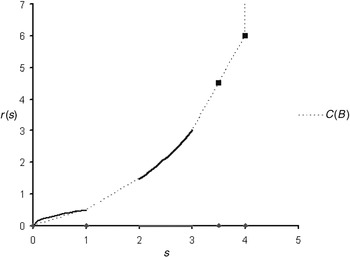
. A subset of the lower boundary of C(B), {(s,r(s))|s ∈ A′}, is called an efficient frontier. Note that this efficient frontier always contains (0,0) and (s,r(s)). Figure 1 illustrates these definitions. Here A′ = {0, 1} ∪ [2,3] ∪ {3.5, 4} and the efficient frontier is {(s,r(s));s ∈ A′}.

Example of A, C(B), and A′.
Our first result shows that there exists an optimal policy that selects a service rate from A′ in all states.
Theorem 3.1: If s ∈ A − A′, then there exists an optimal policy that does not choose s in any state.
Proof: We prove this by contradiction. Suppose a rate s ∈ A − A′ is in fact optimal in some state (x,y) with k + 1 (k ≥ 0) periods to go. Then there must exist

such that

. Since s is optimal in (x,y), we have

It suffices to consider the case where both inequalities are strict since the claim holds trivially otherwise. Applying a little algebra, we get

Defining fk(x,y) = Tp vk(x,y) − vk(x,y) and rewriting the inequalities in terms of fk(x,y), we have


Multiplying (10) by α and (11) by (1 − α) and then adding the two inequalities, we have

This contradicts the fact that

. Therefore, s cannot be optimal. █
Theorem 3.1 implies that it suffices to restrict attention to a minimization problem over A′ instead of A for all states. It also implies that any open interval of feasible rates s for which r(s) is concave need not be considered. When r(s) is concave for all s ∈ A, this result simplifies the optimal service rate decision into a bang-bang control problem.
Corollary 3.1: If r(s) is concave in s, then the optimal service rate s* is either zero or s in all states.
Proof: The result immediately follows from Theorem 3.1 since (0,0) and (s,r(s)) are the only points on the efficient frontier {(s,r(s))|s ∈ A′}. █
Although Theorem 3.1 reduces the set of admissible rates to A′, we still need to solve the optimality equation to find an optimal rate as well as production and inventory policy in each state; that is, for k ≥ 0, the optimal service rate with k + 1 periods to go can be found by solving

Noting that some terms are independent of s, this is equivalent to finding

where Tp vk(x,y) = min[vk(x,y),vk(x + 1,y),vk(x,y − 1{y>0})] and fk(x,y) := Tp vk(x,y) − vk(x,y) ≤ 0. Since r(s) is increasing, it is easy to see that when fk(x,y) = 0, the minimum occurs at s = 0. In addition, sk+1*(x,y) is nonincreasing in fk(x,y), as stated in the following lemma.
Lemma 3.1: Let

for a ≤ b ≤ 0. Then

.
Proof: Suppose

. From the definitions of

, we have

, respectively. Without loss of generality, it suffices to consider the case where at least one of the inequalities holds strictly. Otherwise, the claim holds trivially since one can choose

. Rearranging inequalities, we have

, respectively. Since at least one of the inequalities is strict, this contradicts b ≥ a. Therefore,

. █
For the remainder of this section, we will show that the optimal cost to go function vk(x,y) satisfies a set of properties and that there exists a structured optimal policy for all finite-horizon problems. To do this, we define

to be the set of functions on

satisfying the following properties:
1. v(x + 1,y) ≤ v(x,y − 1) and v(x + 1,y) ≤ v(x,y) for x < 0 and all y > 0.
2. v(x,y) ≤ v(x,y + 1) for all

.
3. (Convexity) For all

:
(i) v(x + 2,y) − v(x + 1,y) ≥ v(x + 1,y) − v(x,y);
(ii) v(x,y + 2) − v(x,y + 1) ≥ v(x,y + 1) − v(x,y).
3. (Submodularity and diagonal dominance) For all

:
(i) v(x + 1,y + 1) − v(x,y + 1) ≤ v(x + 1,y) − v(x,y);
(ii) v(x + 2,y + 1) − v(x + 1,y) ≥ v(x + 1,y + 1) − v(x,y);
(iii) v(x + 1,y + 2) − v(x,y + 1) ≥ v(x + 1,y + 1) − v(x,y).
Note that if

, then

for any scalar c ≥ 0 and that if

, then their sum v + w is also in

. Also note that

. We also define the following operators:

With several technical lemmas and an induction argument, we will show that if

, then there exists a structured optimal policy for the k + 1 stage problem and that

for all k. One might notice that the properties of

are similar to the ones used in Ha [8], where he characterized the structure of the optimal policy for a system with a fixed service rate μ. However, in our problem, the service rate is also a decision variable in the optimality equation; thus, the transition rate at which jobs are completed can vary in state. To use an inductive argument, one must show that the properties of

are preserved in the optimality equation, in particular under two minimization operations: one for the service rate decision and the other for the production and rationing decisions.
Suppose

for some k ≥ 0 (it is certainly true for k = 0). Let Pk(y) be a function in y ≥ 0 such that Pk(y) = min{x ∈ X|vk(x + 1,y) > vk(x,y − 1{y>0})}. Then the following result must hold.
Lemma 3.2: If

for

, then Pk(y) is nonnegative and nonincreasing in y.
Proof: Since

, it follows that vk(x + 1,y − 1) ≤ vk(x + 1,y) ≤ v(x,y) for all x < 0. Thus, Pk(y) ≥ 0 for all y.
To prove that Pk(y) is nonincreasing, first consider when y = 0. Suppose Pk(1) > Pk(0) instead. This implies

This contradicts the fact that

—in particular Property 2, which states that vk is nondecreasing in y. Now suppose there exists y ≥ 1 such that Pk(y + 1) > Pk(y); that is, vk(Pk(y) + 1,y + 1) ≤ vk(Pk(y),y). This inequality and Property 4(iii) imply that

This contradicts the definition of Pk(y); therefore, Pk(y + 1) ≤ Pk(y) for all y ≥ 0. █
Using this lemma, we now characterize the structure of optimal policy for the finite-horizon problem.
Theorem 3.2: If

, there exists an optimal policy for the k + 1 period problem described as follows.
(i) If x < Pk(y), produce to stock (or reduce the class 1 backorder when x < 0). If x ≥ Pk(y) and y > 0, produce to reduce class 2 backorders. Otherwise, do not produce.
(ii) When a class 2 order arrives, satisfy an order immediately from stock if x > Pk(y + 1). Otherwise, place an arriving class 2 order in the backorder queue.
(iii) sk+1*(x,y) = arg mins∈A′{r(s) + sfk(x,y)} is decreasing in x and increasing in y and sk+1*(x − 1,y) ≥ sk+1*(x,y + 1) for x < Pk(y + 1) and all y. Furthermore, if it is optimal not to produce in state (x,y), then sk+1*(x,y) = 0.
Proof:
(i) Consider x < Pk(y). The definition of Pk(y) and Property 2 of

imply that vk(x + 1,y) ≤ vk(x,y − 1{y>0}) ≤ vk(x,y); thus, it is optimal to produce to stock (or reduce class 1 backorders) in state (x,y). If x ≥ Pk(y), then vk(x + 1,y) > vk(x,y − 1{y>0}). For y = 0, do nothing is optimal (i.e., vk(x,0) = Tp vk(x,0)). For y > 0, vk(x,y − 1) ≤ vk(x,y) (Property 2); thus, it is optimal to produce and reduce the class 2 backorder level.
(ii) Since x > x − 1 ≥ Pk(y + 1) ≥ 0, vk(x,y + 1) > vk(x − 1,y); hence, Tr vk(x,y) = min[vk(x,y + 1),vk(x − 1,y)] = vk(x − 1,y). On the other hand, if x ≤ Pk(y + 1), then Tr vk(x,y) = vk(x,y + 1); thus, it is optimal to backorder class 2.
(iii) We first show sk+1*(x,y) is decreasing in x. From Lemma 3.1, it suffices to show fk(x,y) is increasing in x. First, consider the case when y = 0. From the fact that

and claim (i), there are only three cases of the pair (Tp vk(x,0),Tp vk(x + 1,0)) = (min[vk(x,0),vk(x + 1,0)],min[vk(x + 1,0),vk(x + 2,0)]) to consider.
Case a: (Tp vk(x,0) = vk(x,0) and Tp vk(x + 1,0) = vk(x + 1,0)). The result immediately follows because fk(x + 1,0) = fk(x,0) = 0.
Case b: (Tp vk(x,0) = vk(x + 1,0) and Tp vk(x + 1,0) = vk(x + 2,0)). Substituting the corresponding expressions and then applying Property 3(i), we have fk(x + 1,0) − fk(x,0) = vk(x + 2,0) − vk(x + 1,0) − vk(x + 1,0) + vk(x,0) ≥ 0.
Case c: (Tp vk(x,0) = vk(x + 1,0) and Tp vk(x + 1,0) = vk(x + 1,0)). Since vk(x,0) ≥ vk(x + 1,0), fk(x + 1,0) − fk(x,0) = vk(x + 1,0) − vk(x + 1,0) − vk(x + 1,0) + vk(x,0) ≥ 0.
For y > 0, recall that Tp vk(x,y) = min[vk(x + 1,y),vk(x,y − 1),vk(x,y)]. From the fact that

and claim (i), only four distinct feasible cases of (Tp vk(x,y),Tp vk(x + 1,y + 1)) (out of nine possible cases) exist.
Case a: (Tp vk(x,y) = vk(x,y) and Tp vk(x + 1,y) = vk(x + 1,y)). The result holds trivially because fk(x + 1,y) = fk(x,y) = 0.
Case b: (Tp vk(x,y) = vk(x,y − 1) and Tp vk(x + 1,y) = vk(x + 1,y − 1)). fk(x + 1,y) − fk(x,y) = vk(x + 1,y − 1) − vk(x + 1,y) − vk(x,y − 1) + vk(x,y) ≥ 0 (Property 4(i)).
Case c: (Tp vk(x,y) = vk(x + 1,y) and Tp vk(x + 1,y) = vk(x + 2,y)). fk(x + 1,y) = vk(x + 2,y) − vk(x + 1,y) ≥ vk(x + 1,y) − vk(x,y) = fk(x,y) (Property 3(ii)).
Case d: (Tp vk(x,y) = vk(x + 1,y) and Tp vk(x + 1,y)) = vk(x + 1,y − 1). From Property 4(i) and the fact that vk(x + 1,y) ≤ vk(x,y − 1), we have

Thus, fk(x,y) is increasing in x for all y ≥ 0 and sk+1*(x,y) is decreasing in x. The proof for the monotonicity in y is similar and therefore omitted.
We now show that sk+1*(x − 1,y) ≥ sk+1*(x,y + 1) for x < Pk(y + 1). Since Pk(y) is nonincreasing in y, Tp vk(x − 1,y) = vk(x,y) and Tp vk(x,y + 1) = vk(x + 1,y + 1). From Property 4(ii), we get

From Lemma 3.1, sk+1*(x − 1,y) ≥ sk+1*(x,y + 1). Finally, if do nothing is optimal in state (x,y), then fk(x,y) = vk(x,y) − vk(x,y) = 0. Hence, sk+1*(x,y) = 0. █
A policy described in Theorem 3.2 agrees with our intuition that a monotone policy is optimal. For given x, it is optimal to serve class 2 only when the class 2 backorder level exceeds a nonnegative threshold (i.e., x > Pk(y)), which is decreasing in x. To put it differently, it is optimal to produce to raise the stock level for class 1 orders before producing for class 2 backorders. A similar policy is optimal for inventory rationing: Class 1 orders are always rationed from existing stock, but class 2 orders will be served from existing stock only if the system has enough inventory for future class 1 orders. The optimal service rate is monotone in state; that is, sk+1*(x,y) decreases in x but increases in y. The service rate increases as inventory decreases or backorders increase. However, it is rather interesting to note that sk+1*(x − 1,y) ≥ sk+1*(x,y + 1) only when x < Pk(y + 1) instead of for all states. That is because the marginal (inventory and backorder) cost decreases when the state changes from (x + 1,y) to (x,y) for x ≥ Pk(y + 1) ≥ 0, whereas the marginal cost increases for the same transition when there are class 1 backorders (i.e., x < 0).
To show that a structured policy is optimal for all finite-horizon problems, we now only need to show that if

for some

. To see this, suppose

. From Theorem 3.2, there exists a structured optimal policy for the k + 1 stage problem. Applying this argument repeatedly, we get the desired result for any finite-horizon problem. Define an operator (mapping)

, which corresponds to a portion of the value function associated with s:

Then we write the optimality equation for the k + 1 stage problem as

The following two lemmas show that the properties of

are preserved when a function in

is mapped by minimum operators Tr, Tp, and T.
Lemma 3.3: If

, then

.
Proof: The proof is similar to that of Lemma 3.4 and therefore is omitted. █
Lemma 3.4: If

, then

.
Proof: The proof is provided in the Appendix. █
Using these two lemmas, we now show that Properties 1–4 are preserved by the optimality equation.
Theorem 3.3: If

, then

for all k ≥ 0.
Proof: Suppose that

. It is easy to show that

. Also, there exists a structured optimal policy as described in Theorem 3.2 for the k + 1 stage problem, and Tp vk, Tr vk, and

from Lemmas 3.3 and 3.4, respectively. The result then immediately follows from the fact that the class of functions

is closed under multiplication by a nonnegative scalar and the fact that the sum of functions in

are also in

. █
Thus far, we have shown that the optimality equation is in

, and from this, there exists a structured optimal policy for a finite-horizon problem. It is not hard to show that the result can be extended to the infinite-horizon problem.
Theorem 3.4 (Infinite-horizon discounted cost case):
(i)

.
(ii) There exists an optimal policy described by Theorem 3.2 with the exceptions that v(x,y) replaces vk(x,y) and P(y) = min{x : v(x + 1,y) > v(x,y − 1{y>0})} replaces Pk(y).
Proof: The set of functions

is complete under the L∞ metric; thus, the limit of any convergent sequence of functions in

is also in

. Let v∞(x,y) be the limit of any convergent sequence. Theorem 3.2 implies that there exists a structured optimal policy for the one-stage minimization problem with terminal cost v∞(x,y). Furthermore, Properties 1–4 are preserved in the optimality equation for the one-stage problem with terminal value v∞(x,y). By Theorem 5.1 in Porteus [14],

and there exists a structured optimal policy. █
We note that the results also extend to the average cost case by taking the limit of the value function in the discounted cost problem and applying conditions (a)–(g) in Weber and Stidham [17].
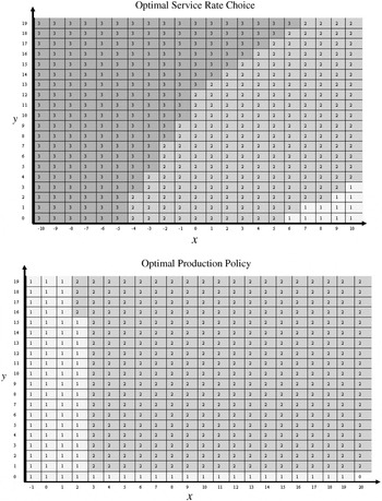
An example of an optimal policy is illustrated in Figure 2. The bottom graph in Figure 2 describes an optimal production policy, which is characterized by a switching curve, P(0) = 20, P(y) = 3 for 0 < y < 16, and P(y) = 2 for y ≥ 16. The top graph in Figure 2 illustrates optimal production rates s*(x,y). As described in our result, the optimal service rate is decreasing in x and increasing in y. Furthermore, for states satisfying x < P(y + 1), monotonicity also holds in the diagonal direction.

Average cost optimal policy at h = 1, b1 = 150, b2 = 50, λ1 = 11, λ2 = 1,μ = 13, and an efficient frontier (s,r(s)) ∈ {(0, 0),(2.0, 0.5),(2.5, 15),(2.8, 100)}.
4. NUMERICAL STUDY
In Section 3 we have shown that an optimal policy is monotone and state dependent. To find an optimal policy, one must solve the optimality equation and simultaneously determine optimal service rate and production (and rationing) decisions for each state. Implementing such an optimal policy can be quite difficult; thus, one might prefer to use a simple heuristic policy if the additional benefit of using an optimal policy is not substantial. In this section we investigate whether the extra efforts of obtaining an optimal policy that dynamically adjusts both capacity and production decisions are well justified.
To answer this question, we conducted a numerical study to compare the optimal policies with three heuristic policies:
Adjustable rate, make-to-order policy (policy AM): Under this policy, we produce for existing orders only and keep no inventory on hand. Priority is given to class 1 orders, and orders in the same class are served under a FIFO discipline. We determine the best service rate in each state and operate the system accordingly.
Adjustable rate, simple base-stock policy (policy AB): We produce until the inventory level reaches a predetermined base-stock level and always serve an arriving order (regardless of its class) from existing stocks. When orders in both classes are backordered, serve class 1 orders first. Given this production policy, we compute the best service rate in each state and operate the system accordingly. We find the best base-stock level by enumeration.
Fixed rate, dynamic production policy (policy FD): Under this policy, we fix the service rate independently of states and find the optimal production (and inventory) policy with respect to a given service rate. We then determine the best service rate by comparing the average cost for all feasible service rates in A′.
The first two policies use a suboptimal production policy but dynamically adjust the service rate based on the congestion level. Policy AM ignores the value of inventory completely, and operates the system as a multiclass queuing system. In policy AB the system produces up to a base-stock level but ignores dynamic rationing. In policy FD the system operates at a fixed service rate, but production (inventory) decisions are dynamically adjusted in the congestion level. Comparing the performance of these policies will highlight the benefit of joint optimal decisions, which we sought in Section 3.
We constructed examples that cover a wide range of scenarios. In all of our examples, we focused on the average cost problems to isolate the effects of planning the horizon and discount factors. For all examples, we assume A′ = {1,2,3}, which means that the system can operate at rate μ, μ + 1, μ + 2, or μ + 3. We fixed the backorder cost for the class 2 order at b2 = 5 and the holding cost at h = 1 and varied other parameters as follows:
- Arrival rates (λ1,λ2): (1,10), (10,1), (1,1);
- Nominal utilization rate (λ1 + λ2)/μ: 0.5, 0.95;
- Backorder cost of class 1 order b1: 10, 100;
- Cost function of additional capacity r(s),s = 1,2,3: Low (0.5, 1.5, 3.0), High (5, 15, 30).
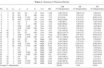
Table 1 summarizes the result of our numerical study. We report the average costs under optimal and three heuristic policies as well as the percentage suboptimality of each heuristic policy. We also report the average suboptimality gaps of all three heuristic policies.
Summary of Numerical Results

Needless to say, policy AM performs extremely poorly in all examples since it ignores future orders and produce all orders in backorder. Although policy AB is substantially better than policy AM, the suboptimality gap is quite significant for some examples. Although policy AB keeps inventory for future orders, it uses the same rationing policy for existing inventory for both demand classes. On the other hand, the optimal policy dynamically changes rationing decisions based on the current state. Under the optimal policy, it might be optimal to keep inventory and class 2 backorders at the same time in order to serve future class 1 orders from existing stock. Class 2 orders are served only when the system has sufficient inventory to serve current and future class 1 orders. Thus, the difference between these two policies measures the benefit of dynamic rationing. The suboptimality gap tends to increase as arrival rate of class 2 orders increases and the difference of backorder costs increases. This shows that considerable savings can be realized from an efficient dynamic production and rationing policy.
We also report that the suboptimality gap between policy FD and the optimal policy can be quite large for a number of examples, particularly when the cost of increasing service rate is high. Since policy FD operates at a constant rate, it incurs unnecessarily high capacity costs when congestion level is low and it fails to ramp up capacity when congestion level is high. Thus, the difference between the two policies represents the benefit of flexibility in capacity (service rate). The results in Table 1 show that both a dynamic capacity decision and a production decision contribute to a substantial reduction of operating cost. Although a simple heuristic policy might be easy to implement, it fails to fully adjust the controls when the current state changes as the optimal policy does.
5. CONCLUSIONS
We have characterized the optimal policy for a make-to-stock production system with an adjustable service rate. We show that under an optimal policy, only service rates on an efficient frontier will be chosen and that a monotone policy is optimal for both service rate and production/inventory decisions. Our contribution is to address a gap in the literature regarding the effective control of make-to-stock systems. With a numerical study we demonstrate that the benefit from joint optimization can be substantial.
Building on our results with two demand classes, we are currently working on several extensions. We are working to extend the result to more than two demand classes and to include a fixed cost for adjusting the service rate. We are also considering models where the decision-maker can change the service rate at random epochs. Such situations arise when additional capacity is provided by workers (machines) who have other primary tasks and will be available to aid only when they are idle. Our preliminary result [11] indicates that an optimal policy might not be monotone and can be of a complex form. Further research will shed light on the structure of an optimal policy.
Acknowledgments
We would like to thank the anonymous referees for helpful comments. The work is partially supported by a National Science Foundation grant (NSF-DMI-0245382).
APPENDIX: Proof of Lemma 3.4
We show that if

, then

is also in

.
Proof for Property 1. For part 1, we show that Tvk(x + 1,y) ≤ Tvk(x,y − 1). Let sp = sk+1*(x,y − 1) and sl = sk+1*(x + 1,y). From Theorem 3.2(iii), sl ≤ sp for x < 0 ≤ Pk(y) ≤ Pk(y − 1). If sp = sl, then the claim holds since

. Now suppose sl < sp. First, note that

Since

. After some algebra, we have

The last inequality holds because sl = arg mins∈A′{r(s) + sfk(x + 1,y)}.
For the second part, let sp = sk+1*(x,y) and sl = sk+1*(x + 1,y). From Theorem 3.2, sp ≥ sl. When sp = sl, it is easy to see that the claim directly follows from Lemma 3 and the assumption that

. Now suppose sp > sl. With some algebra, we get

where the inequality follows from vk(x,y) ≥ vk(x + 1,y) and Tp vk(x,y) ≥ Tp vk(x + 1,y) and the last equality follows from sl = sk+1*(x + 1,y).
Proof for Property 2. Let sp = sk+1*(x,y + 1) and sl = sk+1*(x,y). From Theorem 3.2, sp ≤ sl. Once again, the claim easily follows from Lemma 3.3 and the assumption that

. To see this, suppose sp > sl. We subtract Tvk(x,y) from Tvk(x,y + 1), and with a little algebra, we get

Noting that vk and Tp vk belong to

and that sl minimizes r(s) + sfk(x,y) over s ∈ A′, we have

Proof for Property 3. The fact that Tvk(x,y) is convex in x follows from Properties 4(i) and 4(ii):

On the other hand, Properties 4(i) and 4(iii) together imply convexity in y:

Proof for Property 4.
Property 4(i): Tvk+1(x + 1,y + 1) − Tvk+1(x,y + 1) ≤ Tvk+1(x + 1,y) − Tvk+1(x,y).
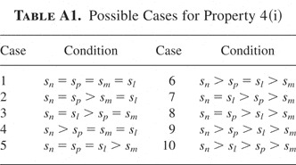
Let sp = sk+1*(x + 1,y + 1), sn = sk+1*(x,y + 1), sm = sk+1*(x + 1,y), and sl = sk+1*(x,y). Theorem 3.2 implies that sn ≥ sp ≥ sm and sn ≥ sl ≥ sm. Thus, there are 10 distinct realizations that satisfy these 2 inequalities, as shown in Table A1.
Table A1: Possible Cases for Property 4(i)

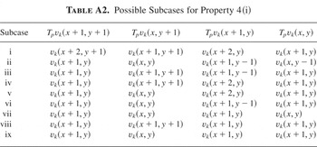
We will show that the claim holds for case 2 (i.e., sn = sp > sm = sl). The proofs for other cases are similar and available upon request. When sn = sp > sm = sl, Theorem 3.2 implies that there are nine possible values of a quadruple: (Tp vk(x + 1,y + 1), Tp vk(x,y + 1), Tp vk(x + 1,y), and Tp vk(x,y)). These values are given in Table A2.
Table A2: Possible Subcases for Property 4(i)

We note that these subcases are not identical in all cases. For example, subcase (vii) cannot occur in cases 3, 5, and 6–10 since sl > 0 implies Tp vk(x,y) ≠ vk(x,y) from Theorem 3.2.
From our assumption that

and Theorem 3.3 (i.e.,

),


For subcases (ii), (v)–(vii), and (ix), [utri ]xTp vk(x,y + 1) = [utri ]x vk(x,y + 1). Thus,

For subcases (i), (iii), (iv), and (viii), first note that [utri ]xTp vk(x,y + 1) = Tp vk(x + 1,y + 1) − vk(x + 1,y + 1). Substituting fk(x + 1,y + 1) = Tp vk(x + 1,y + 1) − vk(x + 1,y + 1), we have

With some algebra and the fact that sp = arg min[r(s) + fk(x + 1,y + 1)] > sl = arg min[r(s) + fk(x,y)],

Property 4(ii): Tvk(x + 2,y + 1) − Tvk(x + 1,y) ≥ Tvk(x + 1,y + 1) − Tvk(x,y).
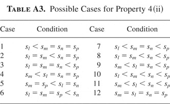
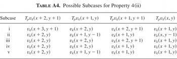
Let sl = sk+1*(x + 2,y + 1), sm = sk+1*(x + 1,y), sn = sk+1*(x + 1,y + 1), and sp = sk+1*(x,y). Theorem 3.2 implies sm ≤ sn, sm ≤ sp, sl ≤ sn; thus, there are 12 feasible cases, as shown in Table A3. We will prove the claim for case 1: sl < sm = sn = sp. Under this case, Table A4 gives the five realizations of (Tp vk(x + 2,y + 1),Tp vk(x + 1,y),Tp vk(x + 1,y + 1),Tp vk(x,y)) that are possible under a policy described in Theorem 3.2.
Table A3: Possible Cases for Property 4(ii)

Table A4: Possible Subcases for Property 4(ii)

Using the fact that

(i.e., [utri ]xyTp vk(x + 1,y) ≥ [utri ]xyTp vk(x,y)) and applying some algebraic manipulation, we have

For subcases (i) and (iii), we note that sp = sm = arg min[r(s) + sfk(x + 1,y)] and get

For subcase (ii), first note that

implies that vk(x + 2,y + 1) − vk(x + 1,y + 1) ≥ vk(x + 1,y) − vk(x,y) (Property 4(ii)) and vk(x + 1,y + 1) − vk(x,y) ≥ vk(x + 1,y) − vk(x,y − 1) (Property 4(iii)). Substituting corresponding expressions in (A.3) yields

Also, note that Tp vk(x + 1,y + 1) = vk(x + 1,y) and Tp vk(x,y) = vk(x + 1,y − 1); thus, [utri ]xyTp vk(x,y) = vk(x + 1,y) − vk(x,y − 1). Using the fact that sp = sm = arg mins∈A′[r(s) + sfk(x + 1,y)], we have

For subcases (iv) and (v), Tp vk(x + 1,y + 1) = vk(x + 1,y) ≤ vk(x + 2,y + 1). Applying this to (A.3), we obtain

Also, note that [utri ]xyTp vk(x,y) = vk(x + 1,y) − vk(x + 1,y) = 0. Thus,

Thus, the claim holds for case 1. The proofs for other cases are similar and are therefore omitted.
Property 4(iii): Tvk(x + 1,y + 2) − Tvk(x,y + 1) ≥ Tvk(x + 1,y + 1) − Tvk(x,y).
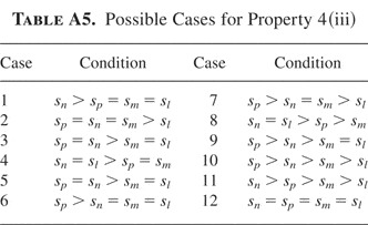
Once again, let sp = sk+1*(x + 1,y + 2), sn = sk+1*(x,y + 1), sm = sk+1*(x + 1,y + 1), and sl = sk+1*(x,y). From Theorem 3.2, it must be true that sp ≥ sm, sn ≥ sl, and sn ≥ sm. There are 12 possible cases that we need to consider. These cases are listed in Table A5.
Table A5: Possible Cases for Property 4(iii)

We will prove case 1: sn > sp = sm = sl. With a little algebra, we have

Rearranging terms and noting that sn = arg mins∈A′[r(s) + sfk(x,y + 1)], the inequality can be further simplified as follows:

The proof for other cases are similar and are therefore omitted.