2. Scale-separated model

The local, ${\delta f}$ gyrokinetic equations describe the evolution of magnetised plasma turbulence driven by mean gradients in the limit that $\rho _{\textrm {th},i}/a \rightarrow 0$ and $\rho _{\textrm {th},e}/a \rightarrow 0$ (Catto Reference Catto1978; Frieman & Chen Reference Frieman and Chen1982; Brizard & Hahm Reference Brizard and Hahm2007); this model is the starting point in the derivation of scale-separated equations for multiscale, electrostatic turbulence (Hardman et al. Reference Hardman, Barnes, Roach and Parra2019). We now briefly review this derivation, first presented in Hardman et al. (Reference Hardman, Barnes, Roach and Parra2019). Ultimately, we find that the local gradients of slowly evolving, long-wavelength turbulence act to modify the mean gradients and flows which drive (or suppress) rapidly evolving, short-wavelength fluctuations. In analogy to the coupling between turbulence and large-scale transport (Sugama & Horton Reference Sugama and Horton1997; Abel et al. Reference Abel, Plunk, Wang, Barnes, Cowley, Dorland and Schekochihin2013), we might expect short-wavelength turbulence to generate fluxes that diffuse long-wavelength turbulence. However, this effect is small by $\left (m_{{e}}/m_{{i}}\right )^{1/2}$ in the ordering, and hence too small to appear at leading order in the $\left (m_{{e}}/m_{{i}}\right )^{1/2}$ expansion that we employ.

In the limit that $\left (m_{{e}}/m_{{i}}\right )^{1/2} \rightarrow 0$, multiscale turbulence can be meaningfully decomposed into components: the long-wavelength ‘ion scale’ (IS) and the short-wavelength ‘electron scale’ (ES). We assume that IS turbulence varies only on $\rho _{\textrm {th},i}$ perpendicular-to-the-field scales in space and on $a/v_{\textrm {th},i}$ scales in time, whereas ES turbulence has much finer $\rho _{\textrm {th},e}$ perpendicular-to-the-field structures, and evolves on the rapid $a / v_{{\textrm {th},e}}$ time scale. Both IS and ES turbulence have parallel-to-the-field scales of order $a$. Here, $\rho _{\textrm {th},p}=v_{\textrm {th},p}/\varOmega _{p}$, with $p$ the particle species index, $v_{\textrm {th},p} = \sqrt {2T_p/m_p}$, $\varOmega _{p} = Z_p e B / m_p c$ the species cyclotron frequency, $T_p$ the species temperature, $Z_p$ the species charge number, $e$ the elementary electric charge, $B$ the magnetic field strength and $c$ the speed of light. The distribution function ${\delta f}$ and electrostatic potential $\phi _{}$ of the turbulence are sums of the IS and ES components:

(2.1a,b)\begin{equation} {\delta f} = {\overline{\delta f}} + {\widetilde{\delta f}}, \quad \phi_{} = \bar{\phi}_{} + \tilde{\phi}_{}, \end{equation}

where $\bar {\chi }$ and $\tilde {\chi }$ are the IS and ES pieces of any quantity $\chi$, respectively. To carry out this decomposition, we introduce the ES average $\langle {\cdot }\rangle ^{\textrm {ES}}$, an average over $\rho _{\textrm {th},e}$ perpendicular-to-the-field scales and $a / v_{{\textrm {th},e}}$ times. We assume that ES turbulence is statistically periodic on $\rho _{\textrm {th},e}$ scales, i.e. $\langle {{\widetilde {\delta f}}}\rangle ^{\textrm {ES}} = 0$. This allows us to use $\langle {\cdot }\rangle ^{\textrm {ES}}$ to extract the scale-separated, coupled gyrokinetic equations for ${\overline {\delta f}}$ and ${\widetilde {\delta f}}$ from the gyrokinetic equations for ${\delta f}$.

The IS component of the turbulence is evolved with the usual gyrokinetic equation for the ion species, and a parallel-orbit-averaged equation for the electron species. The IS turbulence evolves independently of the ES turbulence to leading order in the $\left (m_{{e}}/m_{{i}}\right )^{1/2}$ expansion. At the ES the ion species have a Boltzmann response. The evolution of the ES turbulence is governed by the short-wavelength electron gyrokinetic equation (Hardman et al. Reference Hardman, Barnes, Roach and Parra2019)

(2.2)\begin{align} & \left(\frac{\partial }{\partial {t}} + \bar{\boldsymbol{v}}_{E}\boldsymbol{\cdot} \boldsymbol{\nabla}\right)\tilde{g}_{ } + v_\| \boldsymbol{b} \boldsymbol{\cdot} \boldsymbol{\nabla} \theta \frac{\partial \tilde{g}_{ }}{\partial \theta} + (\boldsymbol{v}_{M} +\tilde{\boldsymbol{v}}_{E}) \boldsymbol{\cdot} \boldsymbol{\nabla} \tilde{g}_{ } + \tilde{\boldsymbol{v}}_{E} \boldsymbol{\cdot} (\boldsymbol{\nabla} F_{0} + \boldsymbol{\nabla} \bar{g}_{ }) \nonumber\\ &\quad =\frac{e F_{0}}{T_{{e}}}\left(v_\| \boldsymbol{b} \boldsymbol{\cdot} \boldsymbol{\nabla} \theta \frac{\partial \tilde{\varphi}_{ }}{\partial \theta} +\boldsymbol{v}_{M} \boldsymbol{\cdot} \boldsymbol{\nabla} \tilde{\varphi}_{ }\right) + \tilde{C}, \end{align}

where we express the ES gyrokinetic equation in terms of the particle guiding centre ${\boldsymbol {R}} = {\boldsymbol {r}} - \boldsymbol {b} \times \boldsymbol {v} / \varOmega _{{e}}$, with ${\boldsymbol {r}}$ the particle position, $\boldsymbol {b}$ the magnetic field direction, $\boldsymbol {v}$ the particle velocity; $\varepsilon$ the particle kinetic energy; $\lambda = \mu / \varepsilon$ the pitch angle, with $\mu$ the magnetic moment; $\sigma$ the sign of the particle velocity in the magnetic field direction $v_\|= \boldsymbol {v}\boldsymbol {\cdot }\boldsymbol {b} = \sigma (2\varepsilon /m_p)^{1/2}(1-\lambda B)^{1/2}$; the gyroaveraged ES potential $\tilde {\varphi }_{ } = \langle {\tilde {\phi }_{}}\rangle ^{\vartheta }_{}$, with $\vartheta$ the angle of gyration about $\boldsymbol {b}$ and $\langle {\cdot }\rangle ^{\vartheta }_{}$ the electron gyroaverage at fixed ${\boldsymbol {R}}$; the ES gyroaveraged electron distribution function $\tilde {g}_{ } = \langle {{\widetilde {\delta f}_{{e}}}}\rangle ^{\vartheta }_{} = \tilde {h}_{} + e \tilde {\varphi }_{ } F_{0} / T_{{e}}$, with ${\widetilde {\delta f}_{{e}}}({\boldsymbol {r}}) = \tilde {h}_{}({\boldsymbol {R}}) + e \tilde {\phi }_{}({\boldsymbol {r}}) F_{0} / T_{{e}}$, $\tilde {h}_{}$ the non-Boltzmann part of the ES electron distribution function and $F_{0}$ the Maxwellian electron mean distribution function. The poloidal angle $\theta$ is the parallel-to-the-field coordinate; $\boldsymbol {v}_{M}$ is the electron magnetic drift; and $\tilde {C}$ accounts for the effects of collisions on $\tilde {g}_{ }$. The long-wavelength and short-wavelength ${{\boldsymbol {E}} \times \boldsymbol {B}}$ drifts are $\bar {\boldsymbol {v}}_{E} = (c/B) \boldsymbol {b} \times \boldsymbol {\nabla } \bar {\phi }_{}$ and $\tilde {\boldsymbol {v}}_{E} = (c/B) \boldsymbol {b} \times \boldsymbol {\nabla } \tilde {\varphi }_{ }$, respectively; and $\bar {g}_{ } = {\bar {\delta f}_{{e}}}$ is the long-wavelength, IS, electron distribution function. Gyroaverages do not appear in the definitions of $\bar {\boldsymbol {v}}_{E}$ or $\boldsymbol {\nabla } \bar {g}_{ }$ as $\rho _{\textrm {th},e}$ is much smaller than the spatial scale of the IS structures. Equation (2.2) is closed by the ES quasineutrality relation $Z_{{i}} \tilde {n}_{{i}} = \tilde {n}_{{e}}$, with $\tilde {n}_{p}$ the ES fluctuating density of species $p$. The ES quasineutrality relation can be written

(2.3)\begin{equation} \int \textrm{d}^3 \boldsymbol{v} |_{{\boldsymbol{r}}} \left( \tilde{g}_{ }({\boldsymbol{R}}) + \frac{e F_{0}}{T_{{e}}}(\tilde{\phi}_{}({\boldsymbol{r}}) - \tilde{\varphi}_{ }({\boldsymbol{R}})) \right) = - \frac{ Z_{{i}} e \tilde{\phi}_{}({\boldsymbol{r}})}{T_{{i}}}n_{0{e}}, \end{equation}

where $n_{0{e}}$ is the mean electron density, and the subscript ${\boldsymbol {r}}$ on the volume element in the velocity space integral indicates that the integral is to be taken at fixed particle position.

Cross-scale interaction is mediated by the terms $\bar {\boldsymbol {v}}_{E} \boldsymbol {\cdot } \boldsymbol {\nabla } \tilde {g}_{ }$ and $\tilde {\boldsymbol {v}}_{E} \boldsymbol {\cdot } \boldsymbol {\nabla } \bar {g}_{ }$ in the electron gyrokinetic equation, (2.2). The gradient $\boldsymbol {\nabla }\bar {g}_{ }$ and the drift $\bar {\boldsymbol {v}}_{E}$ are constant on $a/v_{{\textrm {th},e}}$ time scales, and so appear as additional ‘equilibrium’ terms in the short-wavelength electron gyrokinetic equation. By inspecting (2.2) we see that we are able to ascribe simple physical interpretations to the cross-scale terms: the term $\bar {\boldsymbol {v}}_{E}\boldsymbol {\cdot }\boldsymbol {\nabla } \tilde {g}_{ }$ represents an advection term that will introduce velocity shear; and the gradient $\boldsymbol {\nabla }\bar {g}_{ }$ appears in the term $\tilde {\boldsymbol {v}}_{E}\boldsymbol {\cdot }(\boldsymbol {\nabla }F_{0}+\boldsymbol {\nabla }\bar {g}_{ })$, i.e. 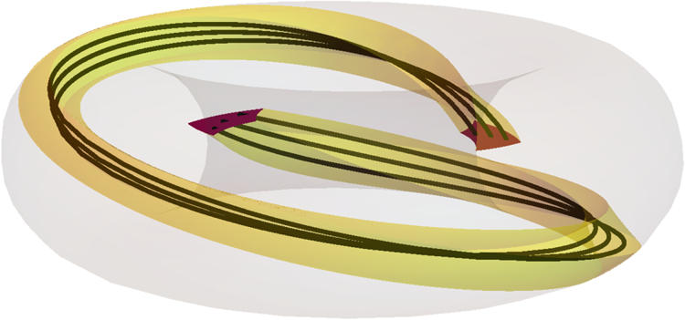$\boldsymbol {\nabla }\bar {g}_{ }$ modifies the usual equilibrium drive of instability $\boldsymbol{\nabla} F _{0}$. Equations (2.2) and (2.3) are solved in a thin ES flux tube embedded within a larger IS flux tube, see figure 1 for an illustration. In each ES flux tube, $\boldsymbol {\nabla } \bar {g}_{ }$ and $\bar {\boldsymbol {v}}_{E}$ take values that are constant in the perpendicular-to-the-field plane; the effects of the perpendicular derivatives of $\boldsymbol {\nabla } \bar {g}_{ }$ and $\bar {\boldsymbol {v}}_{E}$ are small by $\left (m_{{e}}/m_{{i}}\right )^{1/2}$ and so only appear at higher order. However, both $\boldsymbol {\nabla } \bar {g}_{ }$ and $\bar {\boldsymbol {v}}_{E}$ can vary along the field line: this results in a background drive of instability that is no longer uniform in $\theta$, and in suppression of short-wavelength instabilities due to parallel-to-the-field ${{\boldsymbol {E}} \times \boldsymbol {B}}$ shearing by long-wavelength flows. The component of $\bar {\boldsymbol {v}}_{E}$ due to the piece of the electrostatic potential $\bar {\phi }_{}$ that is constant on the flux surface may be removed from (2.2) by boosting to a toroidally rotating frame (Hardman Reference Hardman2019); this component of $\bar {\boldsymbol {v}}_{E}$ can only change the instability frequency by a Doppler shift. We discuss the physical interpretation of these cross-scale interaction mechanisms further in § 4.

Figure 1.

Illustration of a large-scale, IS flux tube with several narrow ES flux tubes embedded within it.

To enable the study of cross-scale interaction in this multiscale framework, the cross-scale terms $\bar {\boldsymbol {v}}_{E} \boldsymbol {\cdot } \boldsymbol {\nabla } \tilde {g}_{ }$ and $\tilde {\boldsymbol {v}}_{E} \boldsymbol {\cdot } \boldsymbol {\nabla } \bar {g}_{ }$ in (2.2) were implemented in the ${\delta f}$ gyrokinetic code GS2 (Kotschenreuther, Rewoldt & Tang Reference Kotschenreuther, Rewoldt and Tang1995; Hardman Reference Hardman2019).

3. Numerical results

In this paper, we address the key question of how the linear stability of the ETG mode is affected by cross-scale interaction. We focus on a plasma in which single-scale microturbulence is well understood: we use a simple magnetic geometry consisting of concentric circular flux surfaces, with parameters largely corresponding to the widely used Cyclone Base Case benchmark (CBC) (Dimits et al. Reference Dimits, Bateman, Beer, Cohen, Dorland, Hammett, Kim, Kinsey, Kotschenreuther and Kritz2000). In the simulations we take $a$ to be the half-diameter of the last closed flux surface; we take the normalised minor radius at the centre of the flux tube $\rho _{0} = r_0/a = 0.54$, with $r_0$ the minor radius of the flux surface; the major radius $R = 3.0 a$; the safety factor at the centre of the flux tube $q_0 = 1.4$; the magnetic shear $\hat {s} = \rho \,\textrm {d} \ln q / \textrm {d} \rho = 0.8$; equal ion and electron temperatures $T_{{i}} = T_{{e}} = T$; the normalised temperature gradient $a/L_{T} = - \textrm {d} \ln T / \textrm {d} \rho = 2.3$; the normalised density gradient $a/ L_n = - \textrm {d} \ln n / \textrm {d} \rho = 0.733$; the normalised self-collision frequencies $a \nu _\textrm {ii} / v_{\textrm {th},i} = a \nu _\textrm {ee} / v_{{\textrm {th},e}} = 10^{-2}$; and the electron-to-deuterium-ion mass ratio $m_{{{e}}}/m_{{{i}}} = 2.7 \times 10^{-4} \approx 1/3670$. In the IS simulations, instead of explicitly implementing the parallel-orbit-averaged equation for the electron species, we impose that the passing, non-zonal electron response is Boltzmann, whilst continuing to solve for the remainder of the electron distribution function with the usual GS2 algorithm. In the limit that $\left (m_{{e}}/m_{{i}}\right )^{1/2} \rightarrow 0$, this has the effect of solving the electron parallel-orbit-averaged equation numerically. The GS2 algorithm employs $(\varepsilon ,\lambda )$ velocity coordinates, and retains the bounce points in $\theta$ for all particles: in this scheme, particles with large parallel velocities have a response that is an orbit average over the fluctuations. To verify that $m_{{{e}}}/m_{{{i}}}= 2.7 \times 10^{-4}$ is sufficiently small for the IS turbulence here to be in the $\left (m_{{e}}/m_{{i}}\right )^{1/2} \rightarrow 0$ limit, we performed additional IS simulations with $m_{{{e}}}/m_{{{i}}} =2.7 \times 10^{-12}$ and a Boltzmann passing, non-zonal electron response. Identical IS fluxes and cross-scale interactions with ETG instabilities were found at $m_{{{e}}}/m_{{{i}}} = 2.7 \times 10^{-12}$ and $m_{{{e}}}/m_{{{i}}} = 2.7 \times 10^{-4}$. Physically, this is because the electron bounce time is shorter than the correlation time of the IS turbulence considered here.

To assess the impact of cross-scale interaction on the ETG instability we carry out the following numerical investigation. We perform simulations of long-wavelength ITG-driven turbulence, using the resolutions detailed in appendix A.1. We compute a sample of $\boldsymbol {\nabla } \bar {g}_{ }(\theta ,\varepsilon ,\lambda ,\sigma )$ and $\bar {\boldsymbol {v}}_{E}(\theta )$ at $6$ times ${t_{{s}}}$, on a $6\times 5$ grid in radial and binormal position, $x_{{s}}$ and $y_{{s}}$, respectively. For each ${t_{{s}}}$ at every sampled $(x_{{s}}, y_{{s}})$ we compute the ETG linear growth rate $\gamma ({t_{{s}}},x_{{s}},y_{{s}})$, including the cross-scale interaction terms $\bar {\boldsymbol {v}}_{E} \boldsymbol {\cdot } \boldsymbol {\nabla } \tilde {g}_{ }$ and $\tilde {\boldsymbol {v}}_{E} \boldsymbol {\cdot } \boldsymbol {\nabla } \bar {g}_{ }$ in (2.2). The resolutions used for the linear calculations are detailed in appendix A.2. 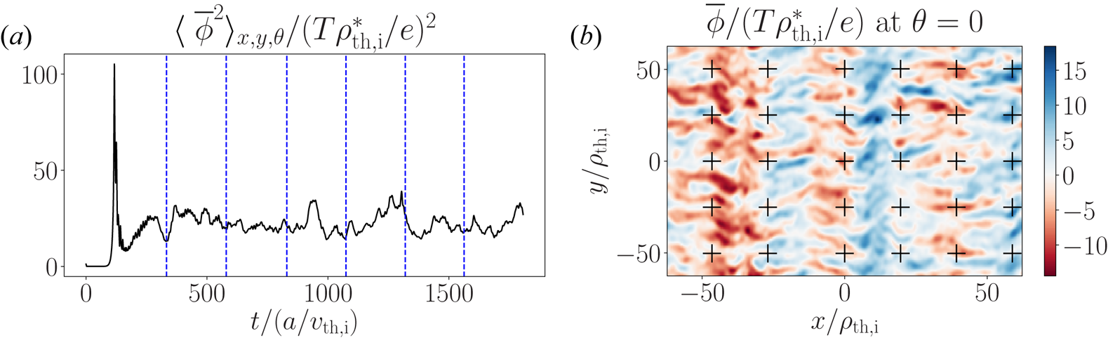This statistical approach is necessary because $\bar {\boldsymbol {v}}_{E}$ and $\boldsymbol {\nabla } \bar {g}_{ }$ must be calculated from turbulent fields which may vary intermittently in time and space. Figure 2(a) shows the spatially averaged IS potential $\langle \, \bar {\phi }_{}^2 \rangle _{x, y, \theta }(t)$, with sampled times indicated with a vertical line; and figure 2(b) shows the IS potential $\bar {\phi }_{}(x,y)$ at the outboard midplane at time $t \simeq 1560 a/v_{\textrm {th},i}$ (the last sampled time in figure 2a), with sampled positions indicated with crosses. The $(x,y)$ coordinates are proportional to the flux-surface and field-line labels, $\psi$ and $\alpha$, respectively, that define the magnetic field $\boldsymbol {B} = \boldsymbol {\nabla } \alpha \times \boldsymbol {\nabla } \psi$: we use the perpendicular-to-the-field coordinates $(x,y)$ that are defined to have units of length, i.e. $x = (\psi -\psi _0) (\textrm {d} \psi / \textrm {d} x)^{-1}$ and $y = (\alpha -\alpha _0) (\textrm {d} \alpha / \textrm {d}y)^{-1}$, respectively, with $(\psi _0,\alpha _0)$ the coordinates of the centre of the IS flux tube, $\textrm {d} \psi / \textrm {d} x = B_{\textrm {ref}} a \rho _{0}/ q_0$ and $\textrm {d} \alpha / \textrm {d}y=B_{\textrm {ref}} a {\partial \rho }/{\partial \psi }|_{\rho _{0}}$, where $B_{\textrm {ref}}$ is a reference magnetic field. We take $B_{\textrm {ref}}$ to be the toroidal magnetic field strength on the flux surface $\psi _0$ at the major radius $R_{\textrm {ref}} = (R_{{\max }} + R_{{\min }})/2$, where $R_{{\max }}$ and $R_{{\min }}$ are the maximum and minimum major radial positions taken in the flux tube, respectively. We note that we choose to define the poloidal angle $\theta$ in the simulations to be such that $\boldsymbol {b} \boldsymbol {\cdot } \boldsymbol {\nabla } \theta$ is constant in $\theta$.

Figure 2.

(a) The IS potential $\bar {\phi }_{}$ in units of $\rho ^{\ast }_{ {\textrm {th},i} } = \rho _{\textrm {th},i}/a$, shown as a function of time (volume-averaged), and (b) at the outboard midplane at $t \simeq 1560 a/v_{\textrm {th},i}$. Times at which the IS turbulence is sampled are indicated with vertical lines, and sampled $(x_{{s}}, y_{{s}})$ positions are indicated by crosses.

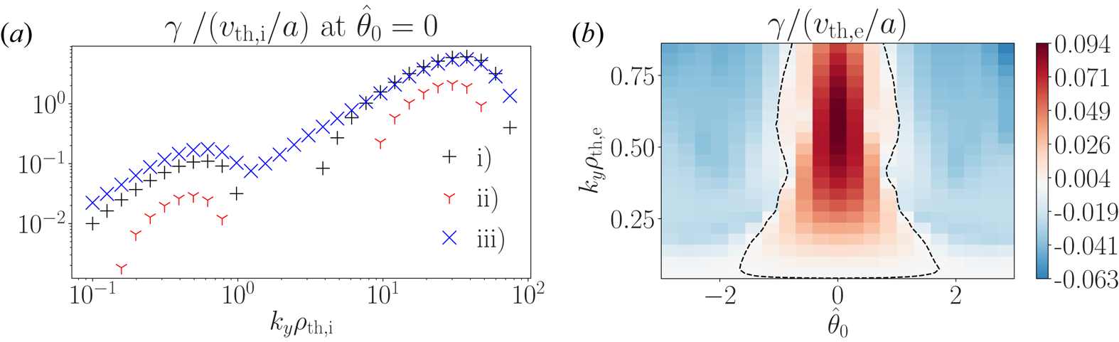
Figure 3 shows the linear growth rate $\gamma$ spectrum in the absence of cross-scale interaction. In figure 3(a) we show $\gamma (k_y)$ for modes with $\hat {\theta }_0 =0$, where $\hat {\theta }_0$ is the poloidal angle at which the wave fronts of the mode align with the minor radial direction of the flux surface. Modes with $\hat {\theta }_0 =0$ have radially aligned wave fronts at the outboard midplane. Figure 3(a) shows that for the simulation parameters used in this paper, see curve (i), there is a natural stable gap in binormal wave number $k_y$ between the ITG and ETG modes: this serves to define the cut-off between the IS and ES. We note that this separation of scales can become larger when both the drives of instability $a/L_{T_{{i}}}$ and $a/L_{T_{{e}}}$ are reduced, see curve (ii), whereas the separation can disappear for sufficiently strong drive or low collisionality, see, e.g., curve (iii). Collisional dissipation creates a stable gap in $k_y$ between the ITG and the ETG modes through the following effects. First, collisional dissipation stabilises both the weakly growing ETG modes with $k_y\rho _{\textrm {th},e} \ll 1$, and the ITG modes with $k_y\rho _{\textrm {th},i} \gtrsim 1$. Second, collisions have the effect of detrapping trapped electrons with an enhanced collision frequency $\nu ^\textrm {detrap}_\textrm {ee} \sim \nu _\textrm {ee}/\epsilon$, where $\epsilon = r_0/R$ is the inverse aspect ratio. When the mode frequency $\omega$ is sufficiently small, i.e. $\omega /\nu ^\textrm {detrap}_\textrm {ee} \lesssim 1$, the trapped electron drive of trapped electron modes (TEMs) (Adam, Tang & Rutherford Reference Adam, Tang and Rutherford1976) and ITG modes is reduced, and hence TEMs and ITG modes that lie in the range $k_y\rho _{\textrm {th},i} \gtrsim 1$ are stabilised, cf. Roach et al. (Reference Roach, Abel, Akers, Arter, Barnes, Camenen, Casson, Colyer, Connor and Cowley2009). In figure 3(b) we plot the full ETG linear growth rate spectrum $\gamma (k_y,\hat {\theta }_0)$ in the absence of cross-scale interaction. Note that the most unstable modes occur at $\hat {\theta }_0 =0$. 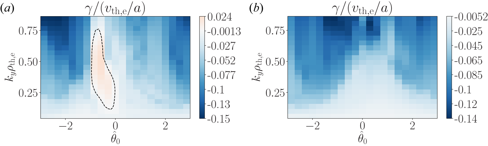The dashed curve in figure 3(b) indicates the stability boundary where $\gamma =0$, calculated with an interpolated spline fit. Figures 4(a) and 4(b) show the ETG growth rates in the presence of cross-scale interactions at two of the sampled IS positions and times. Comparing figure 3(b) with figures 4(a) and 4(b) shows that the effect of cross-scale interaction can be dramatic: in these examples the ETG mode is largely suppressed, and completely stabilised, respectively.

Figure 3.

(a) The linear growth rate without cross-scale effects for three cases: (i) for the parameters given at the start of § 3 ($a/L_{T_{{i}}}=a/L_{T_{{e}}}=2.3$ and $a\nu _{pp} / v_{\textrm {th},p} = 10^{-2}$); (ii) for the case of reduced drive, with $a / L_{T_{{i}}} = a/L_{T_{{e}}}= 1.38$, holding $a\nu _{pp} / v_{\textrm {th},p} = 10^{-2}$; and (iii) for the case of reduced collision frequency, with $a / L_{T_{{i}}} = a / L_{T_{{e}}} = 2.3$ and $a\nu _{pp} / v_{\textrm {th},p} = 10^{-4}$. (b) The ETG growth rate in the absence of cross-scale interaction for the parameters given at the start of § 3 ($a/L_{T_{{e}}} =2.3$ and $a\nu _\textrm {ee} / v_{{\textrm {th},e}} = 10^{-2}$). Modes within the dashed curve are unstable.

Figure 4.

The ETG growth rate in the presence of cross-scale interaction due to IS turbulence: (a,b) show growth rates calculated at different $(x_{{s}}, y_{{s}})$ and times ${t_{{s}}}$. Note the suppression of the growth rate in (a,b) compared with figure 3(b).

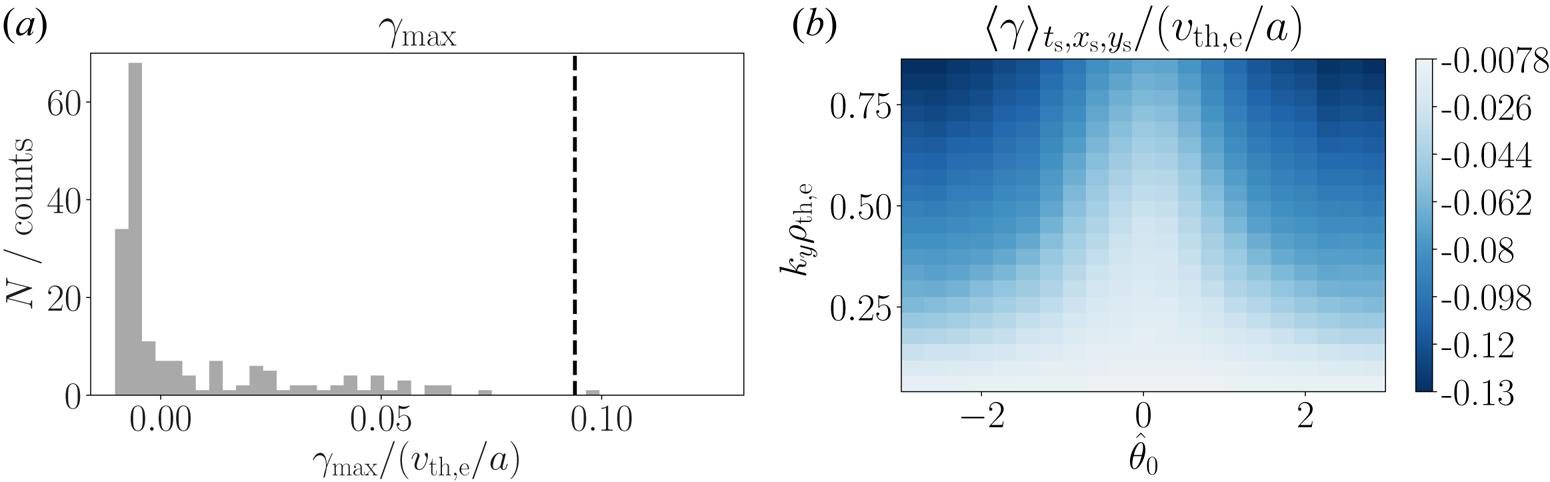
To determine the average, or typical effect of IS turbulence on the ETG instability we calculate the maximum ETG growth rate $\gamma _{{\max }}$ at every $({t_{{s}}},x_{{s}},y_{{s}})$, where we note that the maximum $\gamma$ may occur at a $(k_y,\hat {\theta }_0)$ that is different from the single-scale case. Figure 5(a) shows that the majority of IS drifts and gradients had the effect of stabilising the ETG mode: we find that $\gamma _{{\max }} <0$ at $115$ $({t_{{s}}},x_{{s}},y_{{s}})$ within the sample of $180$, with only a single $({t_{{s}}},x_{{s}},y_{{s}})$ showing a $\gamma _{{\max }}$ larger than the maximum growth rate in the absence of cross-scale interaction. 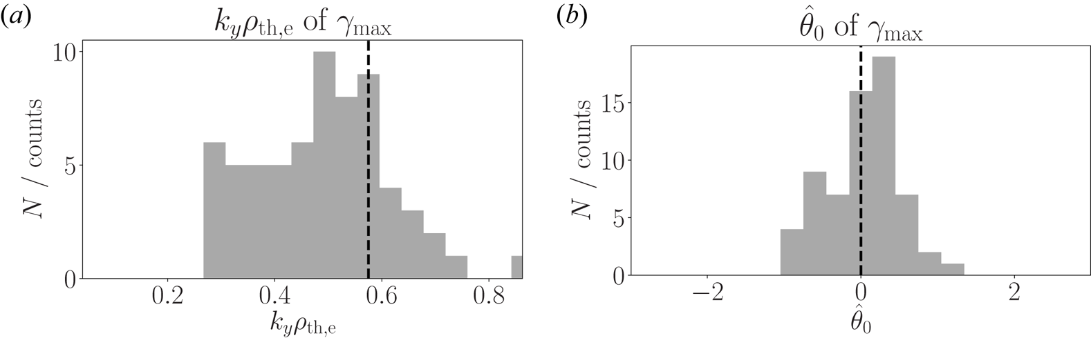This is illustrated further in figure 5(b), which shows that the average of the sampled ETG growth rates $\langle \gamma \rangle _{{t_{{s}}},x_{{s}},y_{{s}}}$ is negative, for all $(k_y,\hat {\theta }_0)$. In figure 6 we show the distributions of $k_y$ and $\hat {\theta }_0$ for the fastest-growing ETG modes in the presence of IS turbulence, with only modes that have $\gamma _{{\max }} > 0$ included in the histograms. Note the significant spread in $k_y$ and $\hat {\theta }_0$ that results from the cross-scale interactions with the IS turbulence.

Figure 5.

(a) The maximum ETG growth rate $\gamma _{{\max }}$ computed including the cross-scale terms $\bar {\boldsymbol {v}}_{E}\boldsymbol {\cdot }\boldsymbol {\nabla }\tilde {g}_{ }$ and $\tilde {\boldsymbol {v}}_{E}\boldsymbol {\cdot }\boldsymbol {\nabla }\bar {g}_{ }$ in (2.2). We see that the typical effect of cross-scale interaction for these parameters is to stabilise the ETG mode. The dashed vertical line indicates the value of $\gamma _{{\max }}$ for the ETG mode in the absence of cross-scale interaction. (b) The average ETG growth rate $\langle \gamma \rangle _{{t_{{s}}},x_{{s}},y_{{s}}}$ as a function of $(k_y,\hat {\theta }_0)$.

Figure 6.

(a) The $k_y$ of the fastest-growing ETG mode. (b) The $\hat {\theta }_0$ of the fastest-growing ETG mode. The dashed lines indicate the $k_y$ and $\hat {\theta }_0$ of the ETG mode in the absence of IS turbulence. Only modes with $\gamma _{{\max }} > 0$ are included in the figures.

These results indicate that strongly driven ITG turbulence can suppress, or stabilise, strongly driven ETG instabilities. This is in agreement with results from multiscale DNS which show reduced short-wavelength heat transport in the presence of strongly driven ITG instabilities, see, e.g., Howard et al. (Reference Howard, Holland, White, Greenwald and Candy2016a,Reference Howard, Holland, White, Greenwald, Candy and Creelyb) and Maeyama et al. (Reference Maeyama, Idomura, Watanabe, Nakata, Yagi, Miyato, Ishizawa and Nunami2015). In the following sections we explore the physical mechanisms that result in the stabilisation of the ETG instability in the $\left (m_{{e}}/m_{{i}}\right )^{1/2} \rightarrow 0$ limit.

4. Physical mechanisms and interpretation

The cross-scale terms in (2.2), $\tilde {\boldsymbol {v}}_{E} \boldsymbol {\cdot } \boldsymbol {\nabla } \bar {g}_{ }$ and $\bar {\boldsymbol {v}}_{E} \boldsymbol {\cdot } \boldsymbol {\nabla } \tilde {g}_{ }$, have intuitive physical interpretations. The gradient $\boldsymbol {\nabla } \bar {g}_{ }$ modifies the local gradients of the background Maxwellian distribution function $\boldsymbol {\nabla } F_{0}$, and thus modifies the instability drive. The drift $\bar {\boldsymbol {v}}_{E}$ is a cross-field flow that advects ES fluctuations and that can vary strongly in the parallel-to-the-field direction. This parallel-to-the-field variation introduces a new parallel length scale and means that $\bar {\boldsymbol {v}}_{E}$ cannot simply be removed from the equations by changing to a rotating or boosted frame. The most unstable toroidal instabilities typically have a parallel wave number $k_\|$ that is set by the connection length $q R$, i.e. $k_\| q R \sim 1$, cf. Parisi et al. (Reference Parisi, Parra, Roach, Giroud, Dorland, Hatch, Barnes, Hillesheim, Aiba and Ball2020). 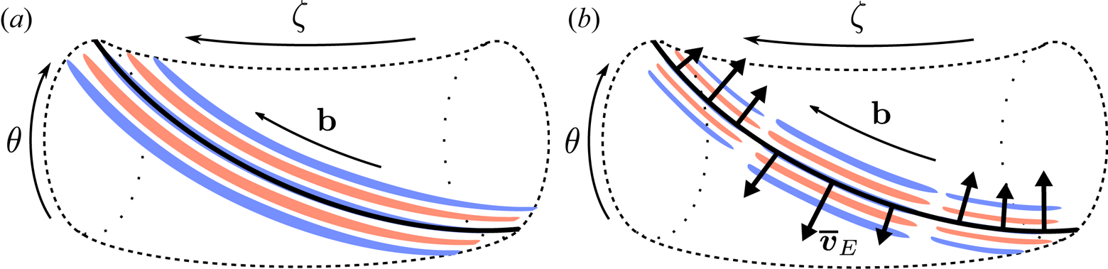Parallel-to-the-field shearing of the ETG fluctuations acts to increase $k_\|$ by imposing a parallel length scale such that $k_\| q R \gtrsim 1$, and hence stabilises toroidal modes. We illustrate the physical picture for parallel-to-the-field shearing in figure 7. Figure 7(a) depicts the field-aligned structure of the toroidal ETG mode in the absence of parallel shearing. Figure 7(b) shows the result of imposing a cross-field flow that varies along the magnetic field line: the $k_\|$ of the ETG mode is now set by the parallel-to-the-field structure of $\bar {\boldsymbol {v}}_{E}$, and not by the connection length $q R$. The drift $\bar {\boldsymbol {v}}_{E}$ varies strongly in the direction of $\boldsymbol {b}$ because at a specific $x_{{s}}$ and $y_{{s}}$ the IS potential $\bar {\phi }_{}=\bar {\phi }_{}(\theta )$. We note that we may express $\boldsymbol {\nabla }\bar {g}_{ } = \boldsymbol {\nabla } \bar {h}_{} + \boldsymbol {\nabla }(e \bar {\phi }_{}/T_{{e}})F_{0}$, with $\bar {h}_{}$ the non-adiabatic response of electrons at IS. In the orbit-averaged model $\bar {h}_{}$ is a constant in $\theta$, at fixed $(\varepsilon ,\lambda )$, and is zero in the passing piece of the velocity space for modes which oscillate in $y$ (non-zonal modes) (Hardman et al. Reference Hardman, Barnes, Roach and Parra2019). Despite this, $\bar {g}_{ }$ can vary strongly in the direction of $\boldsymbol {b}$ because of the contribution from the adiabatic response $e\bar {\phi }_{}F_{0}/T_{{e}}$. Hence, $\boldsymbol {\nabla }\bar {g}_{ }$ contains a contribution to the density gradient $\boldsymbol {\nabla }(e \bar {\phi }_{}/T_{{e}})F_{0}$ that has the effect that the total modified drive of instability $\boldsymbol {\nabla }\bar {g}_{ } + \boldsymbol {\nabla }F_{0}$ drives the mode non-uniformly in $\theta$: this effect can also impose an increased $k_\|$ on the mode. We note that the contribution to $\boldsymbol {\nabla }\bar {g}_{ }$ from the non-adiabatic electron response $\boldsymbol {\nabla }\bar {h}_{}$ contains modifications to the background density and temperature gradients, and gradients of higher-order velocity moments that may drive or suppress instabilities. It is worth noting that the velocity moments of $\bar {h}_{}$ do, in general, depend on $\theta$: this is a consequence of the fact that trapped particles can only access a limited range of $\theta$, and the fact that the non-zonal, passing electron non-adiabatic response vanishes in the orbit-averaged model.

Figure 7.

(a) Cartoon of field-aligned contours of ETG-driven potential fluctuations in the absence of parallel-to-the-field shear. (b) The same ETG-driven mode in the presence of an ${{\boldsymbol {E}} \times \boldsymbol {B}}$ drift that varies in the direction of $\boldsymbol {b}$ on a scale shorter than the connection length by a factor of order unity: the parallel-to-the-field scale of the mode is shortened.

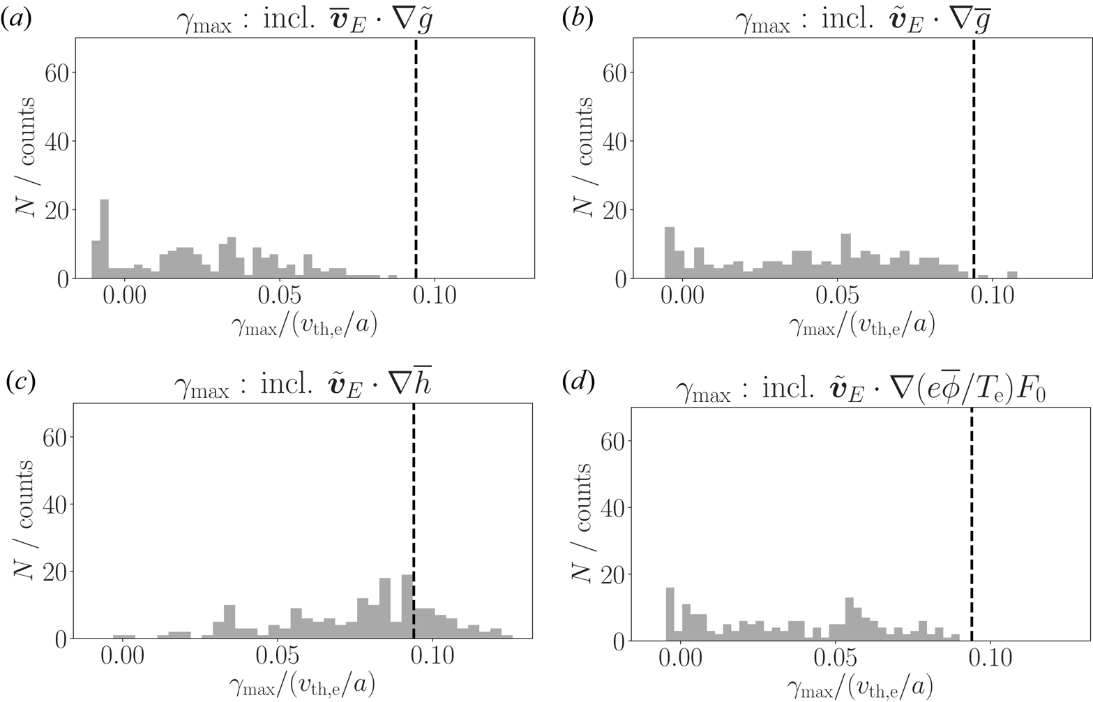
To shed light on the physical mechanisms underlying the result shown in figure 5, we separately consider the effect of including $\boldsymbol {\nabla } \bar {g}_{ }$ and $\bar {\boldsymbol {v}}_{E}$. In figure 8(a) we show the histogram of the maximum ETG growth rate $\gamma _{{\max }}$ computed including only the cross-scale term $\bar {\boldsymbol {v}}_{E}\boldsymbol {\cdot }\boldsymbol {\nabla }\tilde {g}_{ }$ (setting $\boldsymbol {\nabla }\bar {g}_{ }=0$). In figure 8(b) we show the histogram of $\gamma _{{\max }}$ computed including only the cross-scale term $\tilde {\boldsymbol {v}}_{E}\boldsymbol {\cdot }\boldsymbol {\nabla }\bar {g}_{ }$ (setting $\bar {\boldsymbol {v}}_{E}{}=0$). We see by comparing figures 5(a), 8(a) and 8(b) that both the effect of parallel-to-the-field shearing and modifications to the background gradients are important in the ETG stabilisation shown in figure 5. From figure 8(a) we see that the effect of $\bar {\boldsymbol {v}}_{E}$ appears to be uniformly stabilising, i.e. there are no instances where $\gamma _{{\max }}$ becomes larger than the single-scale ETG growth rate. However, in figure 8(b) we see that the effect of $\boldsymbol {\nabla } \bar {g}_{ }$ almost always stabilises the ETG mode, but in rare instances can make the ETG mode more unstable. In the following sections we study these cross-scale physics mechanisms in more detail and provide qualitative explanations for these results.

Figure 8.

Histograms of the maximum ETG growth rate $\gamma _{{\max }}$ computed using (2.2), but including only the cross-scale terms indicated. The dashed vertical line indicates the maximum ETG growth rate in the absence of cross-scale coupling.

We note that our decomposition of the cross-scale terms, while physically motivated, is not unique. In particular, we recall that we can further decompose $\boldsymbol {\nabla } \bar {g}_{ } = \boldsymbol {\nabla } \bar {h}_{} + \boldsymbol {\nabla }(e \bar {\phi }_{}/T_{{e}})F_{0}$. In figures 8(c) and 8(d) we show the cross-scale effects of $\boldsymbol {\nabla } \bar {h}_{}$ and $\boldsymbol {\nabla }(e \bar {\phi }_{}/T_{{e}})F_{0}$ on the ETG mode separately. The piece due to the non-adiabatic response $\boldsymbol {\nabla } \bar {h}_{}$ can both drive and suppress the ETG mode, whereas the piece due to the adiabatic response $\boldsymbol {\nabla }(e \bar {\phi }_{}/T_{{e}})F_{0}$ appears to only suppress the ETG mode. We give a qualitative explanation for this observation in § 6.

5. Evidence for parallel-to-the-field shearing

In this section we show that the physical picture given in figure 7 is consistent with the simulation results presented in § 3: the IS turbulence indeed shortens the parallel-to-the-field scale of the ETG modes. To demonstrate this we first consider the structure of the cross-scale terms and the structure of the ETG eigenmode in the ballooning coordinate, labelled by $\theta$. The fastest-growing ETG mode from a single-scale simulation with CBC parameters occurs at $k_y\rho _{\textrm {th},e} = 0.58$ and $\hat {\theta }_0 = 0$. 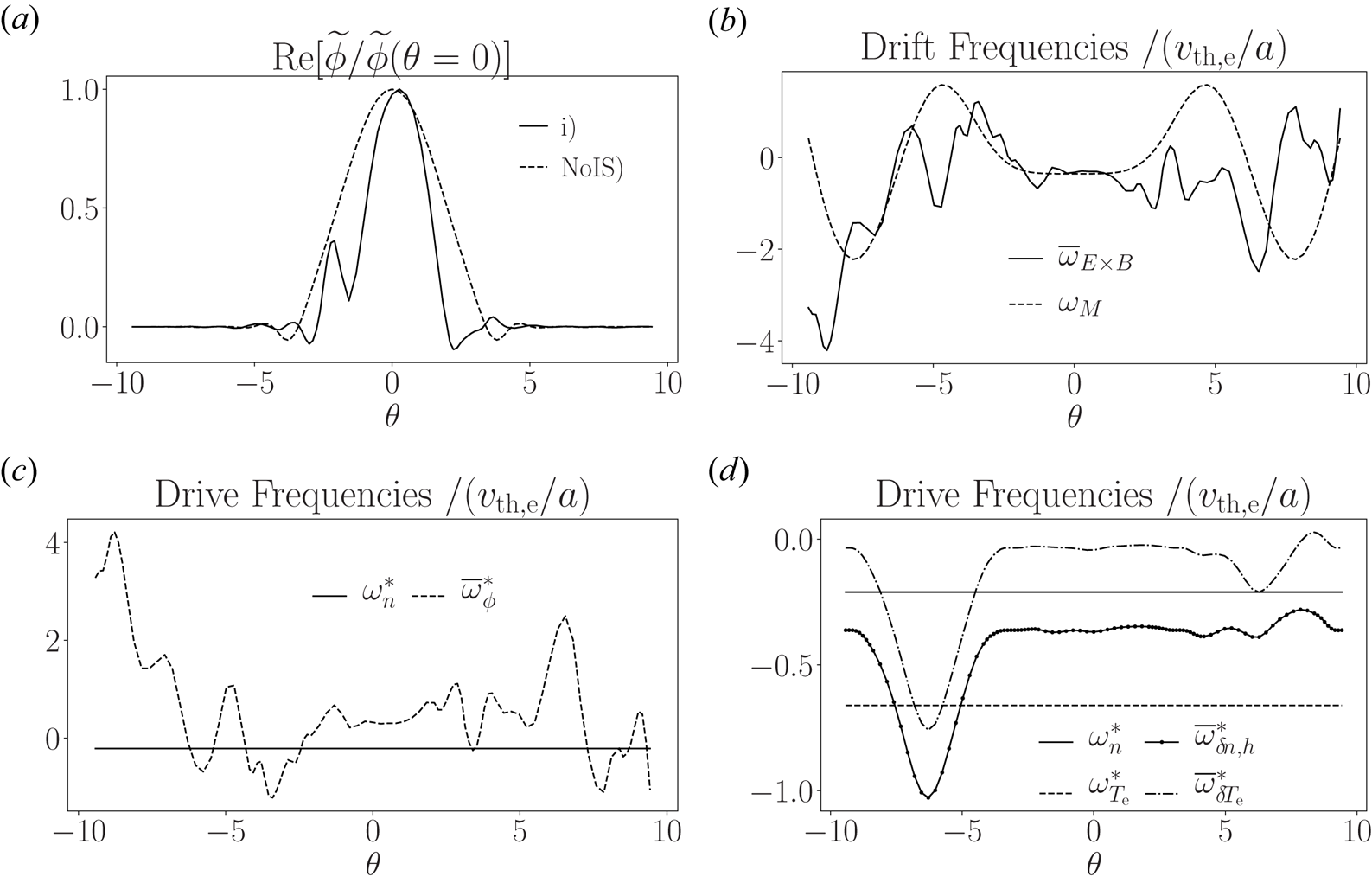Figure 9(a) compares the potential eigenmode for the $k_y\rho _{\textrm {th},e} = 0.58$ and $\hat {\theta }_0 = 0$ mode from a single-scale simulation, to the $k_y\rho _{\textrm {th},e} = 0.58$ and $\hat {\theta }_0 = 0$ mode obtained at a specific example space–time location in the IS turbulence. We see that the cross-scale interaction introduces oscillatory features into the potential eigenmode. This is a result of the variation of $\bar {\boldsymbol {v}}_{E}$ and $\boldsymbol {\nabla } \bar {g}_{ } = \boldsymbol {\nabla } (e \bar {\phi }_{}/T_{{e}}) F_{0} + \boldsymbol {\nabla } \bar {h}_{}$ along the magnetic field line. To illustrate this, in figure 9(b) we show the imposed IS ${{\boldsymbol {E}} \times \boldsymbol {B}}$ drift frequency

(5.1)\begin{equation} \bar{\omega}_{E \times B} = \frac{c \kappa_\rho}{B_{\textrm{ref}}}\left(k_x \frac{\partial \bar{\phi}_{}}{\partial y} - k_y \frac{\partial \bar{\phi}_{}}{\partial x} \right), \end{equation}

with $k_x$ the field-aligned radial wave number of the ETG mode, i.e. the wavenumber $\boldsymbol {k} = k_x \boldsymbol {\nabla } x + k_y \boldsymbol {\nabla } y$, and the geometrical factor $\kappa _\rho = B_{\textrm {ref}}(\textrm {d} x / \textrm {d}\psi )(\textrm {d} y / \textrm {d} \alpha ) \simeq 1.01$ for CBC parameters. The frequency $\bar {\omega }_{E \times B}$ is compared with the thermal magnetic drift frequency

(5.2)\begin{equation} \omega_M = \frac{v_{{\textrm{th},e}}^2}{\varOmega_{{e}}}\boldsymbol{k} \cdot \boldsymbol{b} \times \left( \frac{\boldsymbol{\nabla} B}{B} + \boldsymbol{b} \boldsymbol{\cdot} \boldsymbol{\nabla} \boldsymbol{b} \right). \end{equation}

In figure 9(c) we show the drive frequencies associated with the $\boldsymbol {\nabla } (e \bar {\phi }_{}/T_{{e}}) F_{0}$ piece of $\boldsymbol {\nabla } \bar {g}_{ }$, $\bar {\omega }^{\ast }_{\phi } = - \bar {\omega }_{E \times B}$, compared with the background density gradient drive $\omega ^{\ast }_n = - c k_y T_{{e}} / e B_{\textrm {ref}} L_n$; and in figure 9(d) we show the background temperature gradient drive frequency $\omega ^{\ast }_{T_{{e}}} = - c k_y T_{{e}} / e B_{\textrm {ref}} L_{T_{{e}}}$, and the drive frequencies due to the gradients in the density $\overline {\delta n}_h$ and temperature $\overline {\delta T_{{e}}}$ moments of $\boldsymbol {\nabla } \bar {h}_{}$,

(5.3)\begin{equation} \bar{\omega}^{\ast}_{\delta n,h} = \frac{c \kappa_\rho T_{{e}}}{e B_{\textrm{ref}} }\left(\frac{k_y}{n} \frac{\partial \overline{\delta n}_h}{\partial x} - \frac{k_x}{n} \frac{\partial \overline{\delta n}_h}{\partial y} \right) \end{equation}

and

(5.4)\begin{equation} \bar{\omega}^{\ast}_{\delta T_{{e}}} = \frac{c \kappa_\rho T_{{e}} }{e B_{\textrm{ref}}}\left(\frac{k_y}{T_{{e}}} \frac{\partial \overline{\delta T_{{e}}}}{\partial x} - \frac{k_x}{T_{{e}}} \frac{\partial \overline{\delta T_{{e}}}}{\partial y} \right), \end{equation}

respectively. There are two key feature to note in figures 9(b), 9(c) and 9(d). First, the frequencies that mediate the effects of IS turbulence on ETG modes are comparable in amplitude with the equilibrium drive and thermal magnetic frequencies. Second, the frequencies vary in $\theta$ on the scale of the ETG eigenmode in 9(a). In the strongly driven turbulence that we consider here, we have found that the $\theta$ dependence of $\bar {\omega }_{E \times B}$ cannot be described by a simple function with few parameters. In consequence, simplified quantitative modelling of the effects of parallel-to-the-field shearing by $\bar {\boldsymbol {v}}_{E}$ is challenging. As we discuss in § 6, we find that it is possible to approximate $\bar {\omega }^{\ast }_{\delta n,h}$ and $\bar {\omega }^{\ast }_{\delta T_{{e}}}$ by a constant value.

Figure 9.

(a) The real part of the normalised potential eigenmode for the fastest-growing ETG mode for (i) a specific instance of IS gradients and NoIS) the eigenmode in the absence of cross-scale coupling. The normalised growth rates are $\gamma / (v_{{\textrm {th},e}}/a) = 0.045$ and 0.094, respectively. For simplicity, we chose to compare a case where the fastest-growing mode in the presence of IS turbulence appears at $k_y \rho _{\textrm {th},e} = 0.58$ and $\hat {\theta }_0 = 0.0$. (b) The thermal magnetic drift frequency $\omega _M$ compared to the IS ${{\boldsymbol {E}} \times \boldsymbol {B}}$ drift frequency $\bar {\omega }_{E \times B}$. (c) The drive frequencies due to equilibrium density gradients $\omega ^{\ast }_n$, and due to gradients in the adiabatic part of the IS electron distribution function $\bar {\omega }^{\ast }_{\phi }$. (d) The drive frequencies due to equilibrium temperature gradients $\omega ^{\ast }_{T_{{e}}}$, and gradients of temperature and density in the non-adiabatic part of the IS electron distribution function, $\bar {\omega }^{\ast }_{\delta T_{{e}}}$ and $\bar {\omega }^{\ast }_{\delta n,h}$, respectively.

To assess whether or not the physical picture in figure 7 is consistent with the simulation results, we calculate the $k_\|$ spectrum of the fastest-growing ETG mode at each $({t_{{s}}},x_{{s}},y_{{s}})$ in the sample. For a single ballooning mode, we define the $k_\|$ spectrum to be $|\tilde {\phi }_{}(k_\|)|^2$, where

(5.5)\begin{equation} \tilde{\phi}_{}(k_\|) = \int^{\infty}_{-\infty} \exp[\textrm{i} k_\| z] \tilde{\phi}_{}(z) \,\textrm{d} z, \end{equation}

cf. Parisi et al. (Reference Parisi, Parra, Roach, Giroud, Dorland, Hatch, Barnes, Hillesheim, Aiba and Ball2020), with $z = \theta / \boldsymbol {b} \boldsymbol {\cdot } \boldsymbol {\nabla } \theta$, and $\tilde {\phi }_{}(z)$ is normalised so that the maximum value of $\tilde {\phi }_{}(z)$ is $1$: this maximum may occur away from $z = 0$. 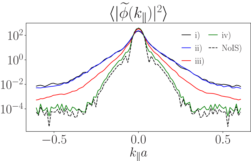We note that we define the $\theta$ coordinate in the simulations such that $\boldsymbol {b} \boldsymbol {\cdot } \boldsymbol {\nabla } \theta$ is constant in $\theta$. In figure 10 we compare $|\tilde {\phi }_{}(k_\|)|^2$ for the fastest-growing ETG mode in the absence of cross-scale interaction with the average $k_\|$ spectrum $\langle |\tilde {\phi }_{}(k_\|)|^2 \rangle$ of the fastest-growing ETG modes in several calculations including various combinations of the cross-scale interaction terms. Figure 10 indicates that cross-scale interaction introduces tails in the $k_\|$ spectra. These tails correspond to the oscillatory structure of the eigenmode shown in figure 9(a). To quantify the size of these tails, we introduce a measure of the spread of the distribution of $k_\|$:

(5.6)\begin{equation} \frac{\sigma_{k_\|}^2}{2} = \frac{\int k_\|^2 \langle |\tilde{\phi}_{}(k_\|)|^2 \rangle \,\textrm{d} k_\|}{ \int \langle |\tilde{\phi}_{}(k_\|)|^2 \rangle \,\textrm{d} k_\|} . \end{equation}

For the fastest-growing ETG mode in the absence of cross-scale interaction $\sigma _{k_\|} = 0.027$. For the average $k_\|$ spectrum of the fastest-growing ETG modes in the presence of all cross-scale interaction terms we find that $\sigma _{k_\|} = 0.065$. This indicates that the effect of cross-scale interaction is indeed to introduce larger $k_\|$ into the ETG mode. Figure 10 indicates that the dominant component of the $k_\|$ tails is introduced by the parallel shearing term $\bar {\boldsymbol {v}}_{E} \boldsymbol {\cdot } \boldsymbol {\nabla } \tilde {g}_{ }$. We also note that the term $\tilde {\boldsymbol {v}}_{E}{}\boldsymbol {\cdot } \boldsymbol {\nabla }\bar {h}_{}$ introduces almost no $k_\|$ component: cross-scale interaction via $\tilde {\boldsymbol {v}}_{E}{}\boldsymbol {\cdot } \boldsymbol {\nabla } \bar {h}_{}$ leaves the form of the ETG eigenmode unchanged. This is consistent with the fact that $\bar {h}_{}$ is constant in $\theta$ at fixed $(\varepsilon ,\lambda ,\sigma ,x,y)$ in the parallel-orbit-averaged model.

Figure 10.

A comparison of the power spectrum of the electrostatic potential $\tilde {\phi }_{}$ of the fastest-growing ETG ballooning mode as a function of $k_\|$ for several cases. In case NoIS) we show the power spectrum of the fastest-growing ballooning mode in the absence of cross-scale coupling. The remaining curves show the $({t_{{s}}},x_{{s}},y_{{s}})$-averaged power spectrum of the fastest-growing ETG mode in the case that: (i) both cross-scale terms $\bar {\boldsymbol {v}}_{E} \boldsymbol {\cdot } \boldsymbol {\nabla } \tilde {g}_{ }$ and $\tilde {\boldsymbol {v}}_{E} \boldsymbol {\cdot } \boldsymbol {\nabla } \bar {g}_{ }$ are included; (ii) only the shearing term $\bar {\boldsymbol {v}}_{E} \boldsymbol {\cdot } \boldsymbol {\nabla } \tilde {g}_{ }$ is included; (iii) only the modification to $\boldsymbol {\nabla } F_{0}$ from the adiabatic response of electrons is included, i.e. $\tilde {\boldsymbol {v}}_{E} \boldsymbol {\cdot } \boldsymbol {\nabla } (e \bar {\phi }_{}/T_{{e}}) F_{0}$; and (iv) only the modification to $\boldsymbol {\nabla } F_{0}$ from the non-adiabatic response of electrons is included, i.e. $\tilde {\boldsymbol {v}}_{E} \boldsymbol {\cdot } \boldsymbol {\nabla } \bar {h}_{}$. To measure the spread of the distribution of $k_\|$ we use $\sigma _{k_\|}$, defined in (5.6). We find (i) $\sigma _{k_\|} = 0.065$, (ii) $\sigma _{k_\|} = 0.064$, (iii) $\sigma _{k_\|} = 0.043$, (iv) $\sigma _{k_\|} = 0.031$ and (NoIS) $\sigma _{k_\|} = 0.027$.

6. Modifications to the drives of instability

The physical interpretation of the impact of $\boldsymbol {\nabla }\bar {g}_{ }$ in (2.2) is that $\boldsymbol {\nabla }\bar {g}_{ }$ modifies the background gradients in $\boldsymbol {\nabla }F_{0}$ that drive the instability. As discussed in § 4, $\boldsymbol {\nabla }\bar {g}_{ }$ is, in general, a complicated function of $(\theta ,\varepsilon ,\lambda )$. In this section we examine to what extent we can model $\boldsymbol {\nabla }\bar {g}_{ }$ by simple modifications to the values of $a/L_{T_{{e}}}$ and $a/L_n$ locally in the IS flux tube. For this we use the results of the simulations presented in figures 8(b), 8(c) and 8(d). This simplified model should be valid when the plasma is collisional and the fluctuations are zonally dominated: in this limit, $\bar {h}_{}$ can be approximated as a perturbed Maxwellian that has no variation within a flux surface. We realise this limiting scenario in § 7.

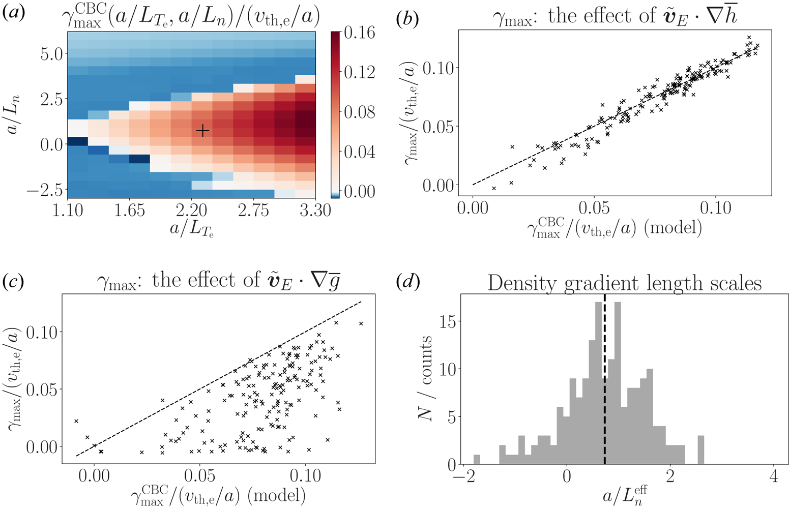
We present the maximum ETG growth rate for the CBC magnetic geometry as a function of the background temperature and density gradients, $\gamma ^{\textrm {CBC}}_{{\max }}(a/L_{T_{{e}}},a/L_n)$, in figure 11(a). We define effective background temperature and density gradients,

(6.1)\begin{gather} \frac{a}{L_{T_{{e}}}^\textrm{eff}} = \frac{a}{L_{T_{{e}}}} - \left\langle{\frac{a \kappa_\rho}{T_{{e}}} \frac{\partial \overline{\delta T_{{e}}}}{\partial x} }\right\rangle_{\theta}, \end{gather}

(6.2)\begin{gather}\frac{a}{L_{n,h}^\textrm{eff}} = \frac{a}{L_n} -\left\langle{ \frac{a\kappa_\rho}{n} \frac{\partial \overline{\delta n}_h}{\partial x} }\right\rangle_{\theta}, \end{gather}

and

(6.3)\begin{equation} \frac{a}{L_{n}^\textrm{eff}} = \frac{a}{L_n} -\left\langle{ \frac{a\kappa_\rho}{n} \frac{\partial \overline{\delta n}}{\partial x} }\right\rangle_{\theta}, \end{equation}

respectively, with $\left \langle {\cdot }\right \rangle _{\theta } = \int ^{{\rm \pi} }_{-{\rm \pi} } \cdot \,\textrm {d} \theta / \boldsymbol {B}\boldsymbol {\cdot }\boldsymbol {\nabla }\theta$ an average in $\theta$ between $(-{\rm \pi} ,{\rm \pi} )$ at fixed $(x,y)$, $\overline {\delta n}_h$ and $\overline {\delta T_{{e}}}$ the density and temperature moments of $\bar {h}_{}$, respectively, and $\overline {\delta n} = \overline {\delta n}_h + ne \bar {\phi }_{} /T_{{e}}$. The normalised density gradient scale $a/L_{n,h}^\textrm {eff}$ measures the effective change to $a/L_n$ by density gradients in the long-wavelength non-adiabatic response of electrons, whereas $a/L_{n}^\textrm {eff}$ measures the effective change to $a/L_n$ by gradients in the total long-wavelength density fluctuation.

Figure 11.

(a) The maximum ETG growth rate for CBC magnetic geometry $\gamma ^{\textrm {CBC}}_{{\max }}$ as a function of the normalised background gradient length scales $a/L_{T_{{e}}}$ and $a/L_n$. The cross indicates the nominal CBC values of $a/L_{T_{{e}}} = 2.3$ and $a/L_n = 0.733$. (b) The maximum ETG growth rate $\gamma _{{\max }}$ including only the effects of the cross-scale term $\tilde {\boldsymbol {v}}_{E} \cdot \boldsymbol {\nabla } \bar {h}_{}$ compared with the model growth rate $\gamma ^{\textrm {CBC}}_{{\max }}(a/L_{T_{{e}}}^\textrm {eff},a/L_{n,h}^\textrm {eff})$. The dashed line indicates the required slope for a perfect correlation. (c) $\gamma _{{\max }}$ including the effects of the cross-scale term $\tilde {\boldsymbol {v}}_{E} \boldsymbol {\cdot } \boldsymbol {\nabla } \bar {g}_{ }$ compared with the model growth rate $\gamma ^{\textrm {CBC}}_{{\max }}(a/L_{T_{{e}}}^\textrm {eff},a/L_{n}^\textrm {eff})$. (d) The histogram of density gradient length scales $a/L_{n}^\textrm {eff}$. The dashed line indicates 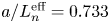$a/L_{n}^\textrm {eff} = 0.733$.

In figure 11(b) we show that there is a strong correlation between the $\gamma _{{\max }}$ calculated using (2.2) including only the cross-scale term due to the IS, non-adiabatic electron response $\tilde {\boldsymbol {v}}_{E} \boldsymbol {\cdot } \boldsymbol {\nabla } \bar {h}_{}$ and the model growth rate $\gamma ^{\textrm {CBC}}_{{\max }}(a/L_{T_{{e}}}^\textrm {eff},a/L_{n,h}^\textrm {eff})$. In contrast, in figure 11(c) we show that the cross-scale interaction due to $\boldsymbol {\nabla }\bar {g}_{ }$ cannot be modelled by $\gamma ^{\textrm {CBC}}_{{\max }}(a/L_{T_{{e}}}^\textrm {eff},a/L_{n}^\textrm {eff})$. Instead, the model $\gamma ^{\textrm {CBC}}_{{\max }}$ almost always overestimates the growth rate of the ETG modes. We can understand these results by referring to figure 10. Cross-scale interaction due to the electron non-adiabatic response $\boldsymbol {\nabla } \bar {h}_{}$ did not change the $k_\|$ spectrum of the ETG eigenmodes: $\boldsymbol {\nabla } \bar {h}_{}$ has the effect of making the mode more or less unstable by changing the drives only. In contrast the difference between $\boldsymbol {\nabla } \bar {g}_{ }$ and $\boldsymbol {\nabla }\bar {h}_{}$, $\boldsymbol {\nabla } (e\bar {\phi }_{}/T_{{e}})F_{0}$, had the effect of introducing larger $k_\|$ components into the mode, which cannot be captured by simple modifications to $a/L_n$ and $a/L_{T_{{e}}}$. The fact that $\gamma ^{\textrm {CBC}}_{{\max }}(a/L_{T_{{e}}}^\textrm {eff},a/L_{n}^\textrm {eff})$ typically overestimates the ETG growth rate in figure 11(c) indicates that the effect of the parallel-to-the-field variation in $\boldsymbol {\nabla } (e\bar {\phi }_{}/T_{{e}})F_{0}$ is stabilising. These results suggest that in general we can characterise $\boldsymbol {\nabla }\bar {g}_{ }$ as having two distinct components: first, a perturbed Maxwellian that simply shifts the equilibrium density and temperature gradients by constant values; and, second, a density gradient from the long-wavelength electron adiabatic response that varies in the parallel-to-the-field coordinate. Whilst the former component may in general stabilise or destabilise the ETG mode, the latter component almost always appears to be stabilising. The effect of $\boldsymbol {\nabla } \bar {g}_{ }$ on an ETG mode depends on the relative importance of these two components.

Finally, we return to the result presented in figure 8(b): the average effect of $\boldsymbol {\nabla } \bar {g}_{ }$ was to suppress ETG instability. We can now understand this result qualitatively. First, the parallel-to-the-field variation in the adiabatic response $\boldsymbol {\nabla } (e\bar {\phi }_{}/T_{{e}})F_{0}$ suppressed the instability by increasing the $k_\|$ in the ETG mode. Second, note that for particular the CBC equilibrium we have chosen, $a/L_n$ maximises the ETG growth rate at fixed $a/L_{T_{{e}}}$, as shown in figure 11(a): any modification to $a/L_n$ will reduce the ETG growth rate $\gamma _{{\max }}$. The histogram of density gradient length scales $a/L_{n}^\textrm {eff}$ shown in figure 11(d) indicates that the typical modification to $a/L_n$ is sufficient to reduce $\gamma _{{\max }}$ by an amount of order unity. This second stabilising effect is likely to be special to this equilibrium.

7. Cross-scale interaction in near-marginal turbulence

The simulation results presented in the previous sections were obtained for parameters where there is a strong background drive of instability for ITG modes at scales comparable with $\rho _{\textrm {th},i}$ and ETG modes at scales comparable with $\rho _{\textrm {th},e}$. In this section, we present results for the case where $a/L_{T_{{i}}}$ and $a/L_{T_{{e}}}$ are reduced so that both the ITG and ETG modes are driven near marginal stability. Weakly driven IS turbulence can reach a Dimits-shift regime where the fluxes are low, and a long-wavelength, long-lived zonal flow regulates the IS dynamics; see, e.g. , Dimits et al. (Reference Dimits, Bateman, Beer, Cohen, Dorland, Hammett, Kim, Kinsey, Kotschenreuther and Kritz2000) and Rogers, Dorland & Kotschenreuther (Reference Rogers, Dorland and Kotschenreuther2000). This represents a very different state from strongly driven, critically balanced, IS turbulence, cf. Barnes, Parra & Schekochihin (Reference Barnes, Parra and Schekochihin2011). Consequently, the relative importance of parallel-to-the-field shearing, parallel-to-the-field variation in the IS density gradient, and constant modifications to the background drives may differ in turbulence driven near marginal stability.

To obtain a near-marginal case, we use the parameters described in § 3, but reduce the normalised background temperature gradient length scales to $a/L_{T_{{e}}} = a/L_{T_{{i}}} =1.38$. We use the resolutions given in appendix A.1, and we take $m_{{{e}}}/m_{{{i}}} =2.7 \times 10^{-12}$ in the IS simulation. The IS turbulence is evolved until a long-lived, zonally dominated state emerges. 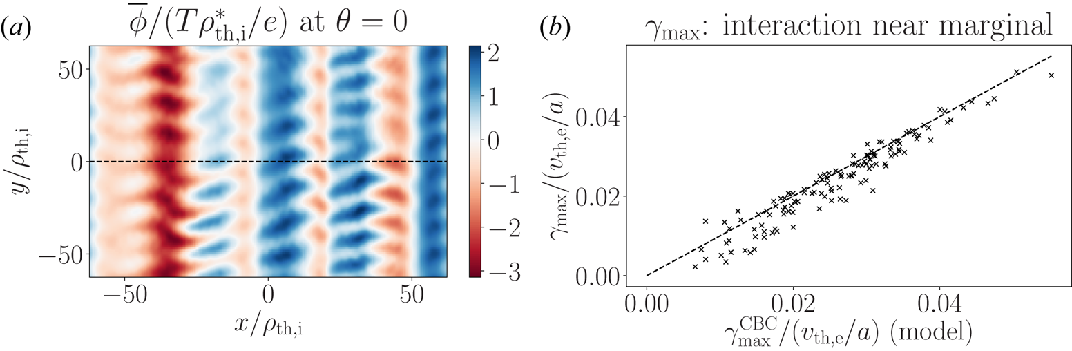We sample the IS gradients $\boldsymbol {\nabla }\bar {g}_{ }$ and drifts $\bar {\boldsymbol {v}}_{E}$ at radial coordinates in the IS flux tube $x_{{s}}$, for a single time ${t_{{s}}}$ and binormal position $y_{{s}}$. In figure 12(a) we show $\bar {\phi }_{}(x,y)$ at ${t_{{s}}}$ for the near-marginal IS turbulence, with the sampled radial points taken along the dashed line. At each of the 128 equally spaced $x_{{s}}$ positions we perform an ETG linear calculation, including the effects of cross-scale interaction via (2.2) and using resolutions detailed in appendix A.2. In contrast to the strongly driven case, in figure 12(b) we show that the maximum growth rate of the ETG mode $\gamma _{{\max }}$, calculated including both cross-scale interaction terms, $\bar {\boldsymbol {v}}_{E} \boldsymbol {\cdot } \boldsymbol {\nabla } \tilde {g}_{ }$ and $\tilde {\boldsymbol {v}}_{E} \boldsymbol {\cdot } \boldsymbol {\nabla } \bar {g}_{ }$, is strongly correlated with the model growth rate $\gamma ^{\textrm {CBC}}_{{\max }}(a/L_{T_{{e}}}^\textrm {eff},a/L_{n}^\textrm {eff})$, with the effective density gradient scales $a/L_{T_{{e}}}^\textrm {eff}$ and $a/L_{n}^\textrm {eff}$ defined in (6.1) and (6.3), respectively, and $\gamma ^{\textrm {CBC}}_{{\max }}$ shown in figure 11(a). The imperfections in the correlation in figure 12(b) are primarily due to parallel-to-the-field shearing from the term $\bar {\boldsymbol {v}}_{E} \boldsymbol {\cdot } \boldsymbol {\nabla } \tilde {g}_{ }$ in (2.2) (cf. figure 10 which shows that $\bar {\boldsymbol {v}}_{E} \boldsymbol {\cdot } \boldsymbol {\nabla } \tilde {g}_{ }$ injects larger $k_\|$ components than $\tilde {\boldsymbol {v}}_{E} \boldsymbol {\cdot } \boldsymbol {\nabla } (e\bar {\phi }_{}/T_{{e}})F_{0}$). We infer that the effect of parallel-to-the-field shearing is weak in this near-marginal turbulence. We verified that the average $k_\|$ spectrum of the fastest-growing eigenmodes was identical in the cases with and without cross-scale interaction.

Figure 12.

(a) Contours of the electrostatic potential $\bar {\phi }_{}(x,y)$ for the sampled near-marginal IS turbulence. The 128 sampled positions $x_{{s}}$ lie equally spaced on the dashed line. (b) The maximum ETG growth rate $\gamma _{{\max }}$ calculated using (2.2), including both cross-scale terms $\bar {\boldsymbol {v}}_{E} \boldsymbol {\cdot } \boldsymbol {\nabla } \tilde {g}_{ }$ and $\tilde {\boldsymbol {v}}_{E} \boldsymbol {\cdot } \boldsymbol {\nabla } \bar {g}_{ }$, compared with the model growth rate $\gamma ^{\textrm {CBC}}_{{\max }}(a/L_{T_{{e}}}^\textrm {eff},a/L_{n}^\textrm {eff})$ that is calculated using the results in figure 11(a) and definitions (6.1) and (6.3). The dashed line indicates the slope for a perfect correlation.

We can understand the result in figure 12(b) with the following intuition. The wavenumber spectrum of near-marginal turbulence is dominated by the zonal mode, a mode that is constant on each flux surface and only depends on the radial coordinate. As a consequence, perpendicular gradients in near-marginal turbulence are dominantly in the radial direction, and the variation of the electrostatic potential $\bar {\phi }_{}$ in the parallel-to-the-field direction in the turbulence is weak. In this regime, the ${{\boldsymbol {E}} \times \boldsymbol {B}}$ advection term $\bar {\boldsymbol {v}}_{E}\boldsymbol {\cdot }\boldsymbol {\nabla }\tilde {g}_{ }$ only modifies the ETG frequency by a Doppler shift (Hardman et al. Reference Hardman, Barnes, Roach and Parra2019). Hence, the dominant cross-scale interaction term that alters the ETG growth rate is due to the radial gradients of the IS electron distribution function, i.e. $\boldsymbol {\nabla }\bar {g}_{ } \simeq \boldsymbol {\nabla } x {\partial \bar {g}_{ }}/{\partial x}$. In addition, if the plasma is sufficiently collisional then $\bar {g}_{ }$ is restricted to be a perturbed Maxwellian of only density and temperature gradients, and in consequence, the effect of cross-scale interaction in near-marginal turbulence may be parameterised with the effective background gradient length scales $a/L_{T_{{e}}}^\textrm {eff}$ and $a/L_{n}^\textrm {eff}$. The results presented in this section demonstrate that this near-marginal cross-scale interaction regime can be realised.