Influences on Election Outcomes

Several factors might influence election outcomes. An impressive body of literature argues that voters look to the state of the economy and vote accordingly (Fiorina Reference Fiorina1981; Key Reference Key1966; Lewis-Beck Reference Lewis-Beck1988; Lockerbie Reference Lockerbie2008). These analyses argue that voters retrospectively evaluate the performance of the economy—if they are pleased, they vote to retain the incumbent party; if they are displeased, they vote to reject the incumbent party. There is an increasing body of evidence that argues that we look to the future when casting a ballot (Lewis-Beck Reference Lewis-Beck2006; Lockerbie Reference Lockerbie2008). This prospective school of thought argues that voters look to the likely economic results of having each party win the upcoming election, then vote for the party that will provide the most prosperous future.Footnote ²

To look at the effects of economic evaluations on election outcomes, I used items from the second quarter of the Survey of Consumer Attitudes and Behavior.Footnote ³ The retrospective item is: “We're interested in how people are getting along financially these days. Would you say that you (and your family living there) are better off or worse off than you were a year ago?” The prospective item is: “Now looking ahead—do you think that a year from now you (and your family living there) will be better off or worse off financially a year from now, or just about the same as now?” In each instance, the score is the percentage responding worse. Unfortunately, these two items are correlated at 0.92, rendering them unfit for simultaneous inclusion in a regression equation.Footnote ⁴ Given this high intercorrelation, I can only make use of one of the two items. Since the prospective items have shown themselves to be more powerful in micro-level analyses (Lewis-Beck Reference Lewis-Beck1988; Lockerbie Reference Lockerbie2008), I have opted to use the prospective item here.

Aside from the economy, we should also take into account the incumbent party's length of service in the White House. As Mueller (Reference Mueller1973) has argued, the longer the incumbent party has held the White House, the greater the opportunity to have upset an increasingly large portion of the electorate. Abramowitz (Reference Abramowitz, Campbell and Garand2000) further argues that regardless of the president's popularity or the state of the economy, there is a desire among the electorate to change control of the White House. When a president gets into office, he must make some decisions very quickly. Those who initially only weakly approved of the president may well see their support wane. Once these weak supporters peel away from the incumbent party, the president's basis of support consists of only hardcore supporters who are more difficult to pull away from the incumbent party. Consequently, I make use of logged time in the White House as my measure.

My equation is atypical amongst the forecasts in that it does not explicitly take into account presidential approval. I specifically exclude presidential approval for two reasons. First, I would argue that the same factors that lead to approval of the president also lead to the election or defeat of the incumbent party. One could build a causal model of forecasting the presidential election, but that might be a bit cumbersome with such a small N. Second, one might argue that including presidential approval is akin to putting a lagged version of the dependent variable on the right-hand side of the equation.

Presidential Election Results

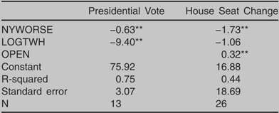
How well does this model do when confronted with the data? The first equation in Table 1 shows the results of a robust regression of the incumbent party's share of the two-party vote on the economic and time in the White House items.Footnote ⁵ The high R-squared (0.75) shows that the model does a reasonably good job of explaining the variation about the mean presidential vote. The coefficients show that every percentage point increase in the number of people responding that they expect the next year to be economically worse leads to approximately a two-thirds of a point loss for the incumbent president's party. Moreover, the economic item is significant at the 0.01 level, one-tailed.Footnote ⁶ Second, the logged time in the White House variable works much like one would expect. Voters tend to be less enthralled with a party the longer it has held the White House.

Table 1.

Forecasting Equations

Note: Estimates are from robust regression.

** significant at 0.01 or better, one-tailed,

* significant at 0.05 or better, one-tailed.

Variables are as described in the text.

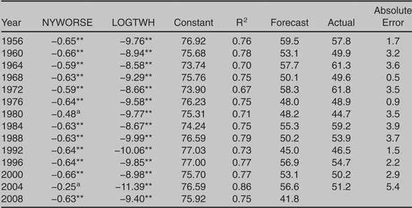
Given the small sample size, it is possible that one case could be dominating the results. Accordingly, that is why the results from the robust regression are so important. While the Cooks' D did not indicate a serious problem with any one case, the Cooks' D for 1980 was 0.25. Table 2 shows the results of out-of-sample forecasting. Briefly, each equation is the same as above, except that the listed year is excluded from the analysis. Then the resulting coefficients from the equation generate a prediction for the excluded year.

Table 2.

Out of Sample Forecasting Equations: Presidential Vote

Note: Estimates are from robust regression. With the exception of 1980 and 2004 Next Year Worse, everything is significant at the 0.01 level one-tailed. Next Year Worse is significant at the 0.12 level one-tailed for 1980. and .23 for 2004.

First, the economic item fares reasonably well. With the exceptions of 1980 and 2004, it remains significant at the 0.01 level, one-tailed. In 1980 and 2004, it is significant at 0.12 and 0.23, respectively.Footnote ⁷ Second, the time variable is even more consistently significant. How good a job does the equation do in terms of actually forecasting the outcome of elections? Overall, the out-of-sample forecasts miscall two of the 13 elections. The equation forecasts a narrow Richard Nixon victory in 1960 and an even narrower Hubert H. Humphrey victory in 1968. In the remaining 11 elections, the equation forecasts the correct popular vote victor. While missing two elections is not a highlight of the equations, one should note that the average error for these two years is less than two percentage points—hardly a tremendous error. The average absolute forecasting error of the model is 2.81 percentage points. The biggest forecasting error is from the 2004 election; the equation missed by over five percentage points.

Looking at 2008, what should we expect? In short, we should see a rather impressive Barack Obama victory. First, a party going for a third term typically has a rough time of it. Second, Americans are amazingly pessimistic about the future of the economy. Fully 23% of Americans are negative about their future personal financial situation. This figure is exceeded only by the percentage in 1980, not an especially good year for the incumbent party. The average on this item is 11.5%. Putting these two pieces of information into the model yields a forecast that McCain will win 41.8% of the two-party popular vote. Given that the largest error to this point is 5.4 percentage points, we should be confident that there is less than 1 chance in 13 that the model incorrectly forecasts an Obama victory.

House Elections

We can forecast legislative elections by adapting the same model that we apply to presidential elections. While we might expect the same variables to be important for forecasting House elections, we should take the differing effect of incumbency on House versus presidential elections into account when making a forecast for that chamber of the legislature. Namely, in House elections incumbents have a tremendous built-in advantage in seeking reelection (Alford and Hibbing Reference Alford and Hibbing1981; Collie Reference Collie1981; Erikson Reference Erikson1972; Ferejohn 1977; Uslaner and Conway Reference Uslaner and Conway1986). Even in 1994, an election year mythologized as an electoral revolution, more than 90% of the incumbents who sought reelection won. If we wish to make a forecast of seat changes in the House, we can safely assume that most incumbents will win. Open-seat contests, however, are where opportunities exist for a party to make gains. Knowing simply the number of open seats is not enough; we must know which party, if either, should be favored.

How do we assess whether any year is favorable for one party? Despite the results of the 1998 and 2002 midterm elections, a midterm loss of seats for the incumbent party has been a regular feature of American politics. How, then, do on-year contests fit into the equation? Are these good years for the party that wins the presidency? That result, of course, occurs after the election, so we could not use it in our forecast. Instead, we want information that is available well before the election we are attempting to forecast. Lewis-Beck and Skalaban (Reference Lewis-Beck and Skalaban1989) show that citizens are reasonably good forecasters of presidential election outcomes. To take into account whether an on-year race is good for a party, we can simply observe whether a disproportionate share (60%+) of the people surveyed forecast a party as the victor. If so, it is a good year for that party. If more than 60% forecast a victory for the incumbent party, then the number of open seats is the score for that variable. If more than 60% forecast a victory for the opposition party, then the number of open seats is multiplied by −1. If the percentage is less than 60 for the party predicted to be victorious, we consider that year to be a wash in terms of open seats switching, and correspondingly score that item a 0. For 1956 through 1992, I made use of the reports from the American National Election Studies. For the more recent elections, I made use of the June reports from the popular press.

How well does the modified presidential forecasting model do with legislative elections? Looking back at Table 1, we can see that it does reasonably well. As with the presidential elections, the prospective economic item is strongly significant. The time in the White House item is spectacularly insignificant. The open-seat item is strongly significant. If it is a bad year for a party, every three open seats leads to a one-seat pickup for the other party. This finding shows both how important incumbency is and that the incumbent party is advantaged when seeking to retain these seats. Nonetheless, these seats appear to be a place where the opposition party can make up some ground. See Table 3.

Table 3.

Out of Sample Forecasting Equations: House Seat Change

Note: Estimates are from robust regression.

** significant at 0.01 or better, one-tailed,

* significant at 0.05 or better, one-tailed. asignificant at 0.06, one-tailed.

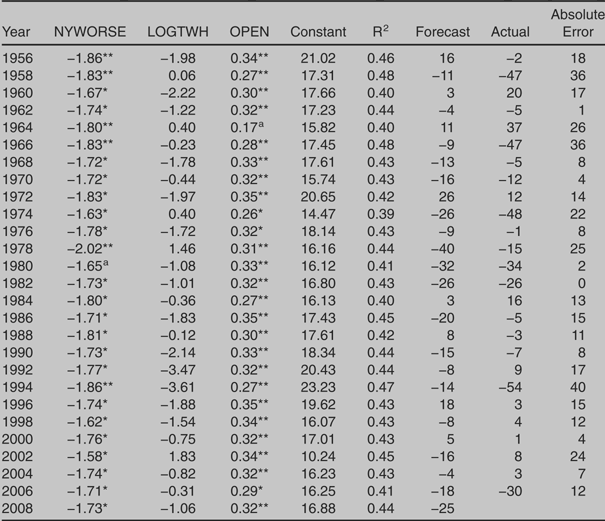
As with the equation forecasting presidential elections, we can also look at the out-of-sample forecasts to evaluate the equation. The prospective economic item is significant at the 0.05 level, one-tailed in every instance but one. In the equation excluding 1980, it is significant at the 0.06 level, one-tailed. The logged time in the White House is still spectacularly insignificant. In no year does it cross the significance threshold. The open-seat item is significant at the 0.05 level, one-tailed in every equation except the one that excludes 1964, where it is significant at the 0.06 level, one-tailed. How good a job does the model do in forecasting seat changes in the House? The R-squared is, on average, 0.43. Second, the average absolute value of the forecasting errors is just over 15 seats. Overall, the model does a respectable, but not quite as good, a job as the presidential equation.

What does the model forecast for the 2008 House elections? Taking the information from earlier (the pessimism of the electorate and the Republicans seeking a third term in the White House) and the fact that less than 60% of voters forecast either candidate to be victorious, the model forecasts a Democratic pickup of 25 seats.