1. INTRODUCTION
The concept of Satellite Formation Flying (SFF) has been well investigated and identified as a key technology for future space operations (Neeck et al., Reference Neeck, Magner and Paules2005; Folta et al., Reference Folta, Bristow, Hawkins and Dell2002), enabling the design of a cluster of simpler, cheaper, and smaller satellites working in unison to achieve specific mission objectives. Compared to a single spacecraft, flying clusters of multiple satellites reduce the risk of an entire mission failing if one system or instrument fails. In addition, formation flying offers various advantages such as the ability to enhance the resolution of observation, improve reliability and flexibility (Kristiansen and Nicklasson, Reference Kristiansen and Nicklasson2009), have lower life cycle costs (Bauer et al., Reference Bauer, Bristow, Carpenter, Garrison, Hartman, Lee, Long, Kelbel, Lu, How, Busse, Axelrad and Moreau2001), and easier expandability (Wei et al., Reference Wei, Park and Park2013). Hence the National Aeronautical and Space Agency (NASA), the European Space Agency (ESA) and other space agencies have shown keen interest in formation flying investigations and various space missions have been proposed (Lawson, Reference Lawson2001; How et al., Reference How, Twiggs, Weidow, Hartman and Bauer1998; Persson et al., Reference Persson, Jacobsson and Gill2005).
Such advantages require a precise formation of spacecraft to make possible applications such as large-scale distributed sensing (radar, interferometry, etc.). It is obvious that the satellites within a formation system are required to synchronise their attitudes while tracking the desired attitudes and angular velocities. However, most of the related studies focused on the control law for attitude synchronisation (Shan, Reference Shan2008; Liu et al., Reference Liu, Shan and Sun2007; Lawton and Beard, Reference Lawton and Beard2002). The attitude synchronisation estimation was not given enough recognition, which is the technical prerequisite for attitude control. Therefore, one should pay more attention to the estimation technique for attitude synchronisation and ensure that it is accurate and robust.
For different space missions, the satellites’ attitude in a formation may need to be adjusted and synchronised with each other. If we can communicate and upload commands with one of the satellites, the others can observe and estimate their attitudes by Charge-Coupled Device (CCD) camera sequentially. This will reduce the work burden for the ground communication system and enhance the autonomous ability of SFF. However, we have to face some problems during this sequential estimation process. The most difficult is that the nonlinear model error from the dynamical model, measurement error of the CCD camera and various kinds of perturbations from space will accumulate from the first satellite to the final satellite, which will seriously hinder attitude estimation performance. Therefore, a new filtering technology with better performance for attitude synchronisation estimation is required.
The Kalman filter and its extended forms (Kalman, Reference Kalman1960; Grewal and Andews, Reference Grewal and Andrews2001; Julier and Uhlmann, Reference Julier and Uhlmann2000; Norgaard et al., Reference Norgaard, Poulsen and Ravn2000; Arasaranam and Haykin, Reference Arasaratnam and Haykin2009) have proven to be extremely useful in a wide range of applications for linear and nonlinear systems. However, the errors in the dynamic system model are treated as “process noise”; therefore, its performance depends not only on the accuracy of the system models, but also on the a priori statistical knowledge of the noise. It is known that the statistical characteristics of the noise are difficult to obtain due to the complex environment (De Ruiter, Reference De Ruiter2010). Especially in the case of nonlinear model error, the model error statistics are not suitable for representation by a zero-mean Gaussian white noise process. In other words, such techniques always have poor ability to address the nonlinear systems with serious model errors. With a view to deal with the model errors, a real-time Predictive Filter (PF) for nonlinear systems was devised based on the research achievements of Lu (Reference Lu1994), Mook and Junkins (Reference Mook and Junkins1988), and further developed by Crassidis et al. (Reference Crassidis, Mason and Mook1993) and Crassidis and Markley (Reference Crassidis and Markley1997a; Reference Crassidis and Markley1997b). This algorithm system can be implemented in real time with an ability to estimate the modelling errors online, which are not restricted only to Gaussian noise. However, the model error weighting matrix in a PF is difficult to choose, and is only chosen based on experience and experiments; hence the practicability and robustness of the PF is decreased. It is evident that the problem mentioned above has seriously restricted the development and application of the PF.
The contribution of this work is the presentation of a novel Predictive Variable Structure Filter (PVSF) and its adaptive form (Adaptive Predictive Variable Structure Filter, APVSF), which are proposed based on Variable Structure Control (VSC) concepts and applied to a nonlinear system with model errors. The proposed PVSF is a type of corrector-predictor estimator without the assumption of “Gaussian process” for the model errors, which has the advantages of estimating the model error to update the system model without the use of precise system representation. However, it has to choose a smoothing boundary layer to address the chattering problem based on the experience. To deal with this shortcoming, the APVSF is further enhanced by the derivative of the posterior covariance with respect to the smoothing boundary layer based on the Mean-Square Error (MSE) principle. This method is more adaptable for practical usage with various kinds of uncertainties, parameter variations, perturbations and so on. It is expected that the proposed methodologies with better filtering performance will be more suitable for attitude synchronisation estimation of the SFF with serious model errors.
The organisation of this paper proceeds as follows. In Section 2 the mathematical model for attitude synchronisation estimation of the SFF is developed. In Section 3 the basic equations and concepts used for the theoretical PVSF are presented with stability proofs. Then, based on the MSE principle, the APVSF is proposed to estimate and adjust the optimal smoothing boundary layer adaptively with detailed analysis in Section 4. Numerical simulations are performed to compare with an Unscented Kalman Filter (UKF) to demonstrate the accuracy and robustness of the two proposed methods, which also illustrate that the PVSF theory is more suitable for attitude synchronisation estimation of the SFF in Section 5. Some conclusions are drawn in the final section.
2. EQUATIONS GOVERNING THE ATTITUDE SYNCHRONISATION ESTIMATION OF THE SFF
For simplicity, the relative attitude motion of the SFF with two satellites is described, on which basis the relative attitude of the SFF with multiple satellites can be obtained. The related coordinate frames are defined first. The inertial frame (I): the J2000 Equatorial Reference Frame. The Relative Motion (RM) frame: a Cartesian right-handed reference frame fixed to the chief satellite's centre of mass (c.m.), with the x -axis directed from the satellite radially outward, the z -axis along the normal to the chief satellite's orbital plane, and the y -axis completing the triad. The Body Fixed (BF) frame: a Cartesian right-handed coordinate system attached to the deputy's c.m. In this paper,
 ${\bi a}^N $
denotes the vector
 ${\bi a}$
expressed in frame N, and
 $\left. {\dot {\bi a}} \right\vert_N $
denotes the time derivative of vector in the frame N.
Using quaternions to represent the relative attitude of the BF frame relative to the RM frame, the kinematic differential equation can be written as
 $$\dot{\bi q} = \displaystyle{1 \over 2}{\bi \Omega} \left( {\bi \omega} \right){\bi q} = \displaystyle{1 \over 2}{\bi E}_1 \left( {\bi q} \right){\bi \omega} $$
where,
 ${\bi q} = \left[ {q_1, q_2, q_3, q_4} \right]^T $
and
 ${\bi \omega} = \left[ {\omega _1, \omega _2, \omega _3} \right]^T $
are the relative attitude quaternions and the angular velocity of the BF frame with respect to the RM frame. Here q
1 is the scalar part and
 $q_i, \matrix{ {} \cr} i = 2,3,4$
is the vector part and q
24 = [q
2, q
3, q
4]
T
, while
 ${\bi \Omega} \left( {\bi \omega} \right)$
,
 ${\bi E}_1 \left( {\bi q} \right)$
are defined by
 $${\bi \Omega} \left( {\bi \omega} \right) = \left[ {\matrix{ 0 & { - {\bi \omega} ^T} \cr {\bi \omega} & { - \left[ {{\bi \omega} \times} \right]} \cr}} \right],\matrix{ {} \cr} \matrix{ {} \cr} {\bi E}_1 \left( {\bi q} \right) = \left[ {\matrix{ { - q_{24}^T} \cr {q_1 I_{3 \times 3} + \left[ {q_{24} \times} \right]} \cr}} \right],\matrix{ {} \cr} \matrix{ {} \cr} \left[ {{\bi \omega} \times} \right] = \left[ {\matrix{ 0 & { - \omega _3} & {\omega _2} \cr {\omega _3} & 0 & { - \omega _1} \cr { - \omega _2} & {\omega _1} & 0 \cr}} \right]$$
The relative angular velocity of the BF with respect to the RM can be expressed as
 $${\bi \omega} = {\bi \omega} _d - {\bi A}\left( {\bi q} \right){\bi \omega} _o^{RM} $$
where
 ${\bi \omega} _d $
is the angular velocity of the deputy satellite (BF) with respect to the inertial frame,
 ${\bi \omega} _o^{RM} $
is the angular velocity of the chief satellite (RM) with respect to the inertial frame, in the form of
 ${\bi \omega} _o = \left[ {\omega _{ox}, 0,\omega _{oz}} \right]^T $
.
 ${\bi A}\left( {\bi q} \right)$
is the transformation matrix from the RM frame to the BF frame, and can be expressed as
 $${\bi A}\left( {\bi q} \right) = \left[ {\matrix{ {q_1^2 + q_2^2 - q_3^2 - q_4^2} & {2\left( {q_2 q_3 + q_1 q_4} \right)} & {2\left( {q_2 q_4 - q_1 q_3} \right)} \cr {2\left( {q_2 q_3 - q_1 q_4} \right)} & {q_1^2 - q_2^2 + q_3^2 - q_4^2} & {2\left( {q_1 q_2 + q_3 q_4} \right)} \cr {2\left( {q_2 q_4 + q_1 q_3} \right)} & {2\left( {q_3 q_4 - q_1 q_2} \right)} & {q_1^2 - q_2^2 - q_3^2 + q_4^2} \cr}} \right]$$
Differentiation of Equation (3) in the inertial frame (I) yields
 $$\left. {\dot{\bi \omega}} \right \vert _I = \left. { \dot{\bi \omega}} \right \vert _{RM} \,+\, {\bi \omega} _o \times {\bi \omega} = \left. { \dot{\bi \omega} _d} \right \vert _I - {\bi A}\left( {\bi q} \right)\left( {\left. { \dot{\bi \omega} _o} \right \vert _I} \right)^{RM} $$
Euler's equations describing the rotational motion of the deputy satellite are given by
 $$\left. {{\bi J}_d \dot{\bi \omega} _d} \right \vert _I \,+\, {\bi \omega} _d \times {\bi J}_d {\bi \omega} _d = {\bi T}_d + {\bi d}_1 $$
where
 ${\bi J}_d $
is the inertia tensor of the deputy,
 ${\bi T}_d $
is the external torque,
 ${\bi d}_1 $
represents the uncertain model errors of the system and perturbations from the space, which is not restricted to be Gaussian.
Using Equations (3), (5) and (6) and expressing the result in the BF frame with the superscript and subscript (I) omitted for convenience, one obtains after some algebra,
 $$\eqalign{\dot{\bi \omega} & = {\bi J}_d^{ - 1} \left( {{\bi T}_d - \left( {{\bi \omega} + {\bi A}\left( {\bi q} \right){\bi \omega} _o^{RM}} \right) \times {\bi J}_d \left( {{\bi \omega} + {\bi A}\left( {\bi q} \right){\bi \omega} _o^{RM}} \right)} \right) \cr &\quad - {\bi A}\left( {\bi q} \right) \dot{\bi \omega} _o^{RM} - \left( {{\bi A}\left( {\bi q} \right){\bi \omega} _o^{RM}} \right) \times {\bi \omega} + {\bi J}_d^{ - 1} {\bi d}_1} $$
Hence, we can obtain the relative rotational dynamics between two satellites of the SFF based on Equation (1) and Equation (7). For SFF with multiple satellites, we can assume that the satellite communicating with the ground station is labelled with number “1”, the desired control attitude is represented by number “0”, and the other satellites are labelled with numbers “2,3…n” from the near to far end sequentially. The relative attitude between the satellites can be observed or measured by a CCD camera and
 $i \to j,\matrix{ {} \cr} i,\,j = 0,1,2 \cdots n,\matrix{ {} \cr} i \ne j$
represents the relative variables between satellite i and satellite j. Based on the above assumptions, the relative rotational dynamics between any two satellites of the SFF can be expressed by
 $$\eqalign{\dot{\bi q}_{i \to j} & = \displaystyle{1 \over 2}{\bi \Omega} \left( {{\bi \omega} _{i \to j}} \right){\bi q}_{i \to j} = \displaystyle{1 \over 2}{\bi E}_1 \left( {{\bi q}_{i \to j}} \right){\bi \omega} _{i \to j} \cr & \dot{\bi \omega} _{i \to j} = {\bi J}_i ^{ - 1} \left( {{\bi T}_i - \left( {{\bi \omega} _{i \to j} + {\bi A}\left( {{\bi q}_{i \to j}} \right){\bi \omega} _o^{RM}} \right) \times {\bi J}_i \left( {{\bi \omega} _{i \to j} + {\bi A}\left( {{\bi q}_{i \to j}} \right){\bi \omega} _o^{RM}} \right)} \right) \cr &\quad\qquad - {\bi A}\left( {{\bi q}_{i \to j}} \right) \dot{\bi \omega} _o^{RM} - \left( {{\bi A}\left( {{\bi q}_{i \to j}} \right){\bi \omega} _o^{RM}} \right) \times {\bi \omega} _{i \to j} + {\bi J}_i ^{ - 1} {\bi d}_i} $$
The optical imaging system of the CCD camera is employed as the measurement sensor. It is assumed that the output of the CCD vision measurement unit gives the relative attitude information directly. Therefore the observation model of the CCD is given as follows:
 $$\left\{ \matrix{\phi = \phi ^{\prime} + v_\phi \hfill \cr \theta = \theta ^{\prime} + v_\theta \hfill \cr \psi = \psi ^{\prime} + v_\psi \hfill} \right.$$
where φ, θ, ψ represent the output relative attitude angles from the CCD sensor, φ′, θ′, ψ′ represent the actual values, v
φ
, v
θ
, v
ψ
are the measurement noises of the CCD sensor. Although the system model noise
 ${\bi d}_i $
can be non-Gaussian, the measurement noises are typically Gaussian. Hence, v
φ
, v
θ
, v
ψ
have been assumed to be Gaussian with zero mean and covariance
 ${\bi R}$
.
Because the relative rotational dynamics are expressed by quaternions in Equation (8), we assume that the CCD vision measurement unit has the facility to transfer the relative attitude angles to quaternions. Based on Equation (9), the observation model used in this paper can be expressed as
 $${\bi y} = {\bi h}\left( {\bi X} \right) = {\bi q}_{i \to j} $$
where
 ${\bi q}_{i \to j} $
is the measurement relative quaternion with noise.
3. PREDICTIVE VARIABLE STRUCTURE VARIABLE FILTER
3.1. The proposed PVSF
In this section, the nonlinear Predictive Variable Structure Filter (PVSF) algorithm is derived. It can estimate the model error to update the system model with high accuracy first, then improve the state estimates. To derive the PVSF algorithm, a nonlinear discrete-time system is considered to be represented by the following equation with model error:
 $$\eqalign{{\bi x}_{k + 1} & = {\bi f}\left( {{\bi x}_k} \right) + {\bi g}\left( {{\bi x}_k} \right){\bi d}_k \cr {{\bi y}_k}& = {\bi h}\left( {{\bi x}_k} \right) + {\bi v}_k} $$
where k ∈ N
0 is the discrete time,
 ${\bi f}( {\cdot}\! ) \in {\opf R}^n $
and is a sufficiently differentiable vector field and ℝ
n
is the real n-dimensional vector space,
 ${\bi x}_k \in {\opf R}^n $
is the system state vector,
 ${\bi d}_k \in {\opf R}^p $
is the model error vector which can be non-Gaussian, and
 ${\bi g}({\cdot}\!) \in {\opf R}^{n \times p} $
is the model error distribution matrix, which determines how the model error is introduced into the plant dynamics. Furthermore,
 ${\bi y}_k \in {\opf R}^m $
is the measurement vector,
 ${\bi h}({\cdot}\!) \in {\opf R}^m $
is a sufficiently differentiable vector field,
 ${\bi v}_k \in {\opf R}^m $
represents the measurement noise vector, which is assumed to be white-noise Gaussian with zero-mean and covariance
 ${\bi R}$
.
In the nonlinear PVSF, it is assumed that the state and output estimates are given by a preliminary model and a to-be-determined model error vector, given by
 $$\eqalign{{\hat {\bi x}}_{k + 1} & = {\bi f}\left( {{\hat{\bi x}}_k} \right) + {\bi g}\left( {{\hat {\bi x}}_k} \right){\bi d}_k \cr {\hat{\bi y}_k}&= {\bi h}\left( {{\hat {\bi x}}_k} \right)} $$
Considering the Lie derivative (Slotine and Li, Reference Slotine and Li1991) as defined by
 $$\eqalign{L_f^k \left( {{\bi h}_i} \right) & = {\bi h}_i, \matrix{ {} \cr} \matrix{ {} \cr} for\matrix{ {\matrix{ {} \cr}} \cr} \matrix{ {} \cr} k = 0 \cr L_f^k \left( {{\bi h}_i} \right) & = \displaystyle{{\partial L_f^{k - 1} \left( {{\bi h}_i} \right)} \over {\partial {\bi x}_t}} f\left( {{\bi x}_t} \right),\matrix{ {} \cr} \matrix{ {} \cr} for\matrix{ {\matrix{ {} \cr}} \cr} \matrix{ {} \cr} k \ge 1 \cr L_{g_j} L_f^k \left( {{\bi h}_i} \right) & = \displaystyle{{\partial L_f^k \left( {{\bi h}_i} \right)} \over {\partial {\bi x}_t}} {\bi g}_j \left( {{\bi x}_t} \right)} $$
where
 ${\bi g}_j $
is the jth column of
 ${\bi g}\left( {{\bi x}_t} \right)$
and
 ${\bi h}_i $
the ith component of
 ${\bi h}\left( {{\bi x}_t} \right)$
. A Taylor series expansion of the output in Equation (11) is given by
 $${\bi y}_{k + 1} = {\bi y}_k + {\bi Z^{\prime}}\left[ {{\bi x}_k, \Delta t} \right] + {\bi \Lambda} \left( {\Delta t} \right){\bi U}\left[ {{\bi x}_k} \right]{\bi d}_k + o\left( {{\bi e^{\prime}}_{k + \Delta t}} \right)$$
where Δt is the sampling interval and
 $o\left( {{\bi e}_{k + \Delta t}} \right) = {\bi \varepsilon} \left[ {{\bi x}_k, {\bi d}_k} \right] + {\bi v}_{k + 1} $
,
 ${\bi \varepsilon} \left[ {{\bi x}_k, {\bi d}_k} \right]$
is the high-order discretisation error,
 ${\bi U}\left[ {{\bi x}_k} \right] \in {\opf R}^{m \times p} $
is a matrix given by
 $${\bi U}_{ij} \left[ {{\bi x}_t} \right] = L_{g_j} L_f^{r_i - 1} {\bi h}_i \left[ {{\bi x}_k} \right],\matrix{ {} \cr} \matrix{ {} \cr} i = 1,2, \cdots, m,\matrix{ {} \cr} j = 1,2, \cdots, p$$
 ${\bi \Lambda} \left( {\Delta t} \right)$
is a diagonal matrix with its diagonal elements λ
ii
as follows
 $$\lambda _{ii} = {{\Delta t^{r_i}} / {r_i !}},\matrix{ {} \cr} \matrix{ {} \cr} i = 1,2, \cdots, m$$
 ${\bi Z}_i ^{\prime} \left[ {{\bi x}_k, \Delta t} \right]$
is a vector
 $${{\bi Z}_i}{\rm }\left[ {{{\bi x}_k},\Delta t{\rm }} \right] = \sum\limits_{l = 1}^{{r_i}} {\displaystyle{{\Delta {t^{{k^{\prime}}}}} \over {l!}}} L_f^l \left( {{{\bi h}_i}} \right),\quad i = 1,2, \cdots ,m$$
and r
i
satisfies
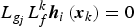 $L_{g_j} L_f^k {\bi h}_i \left( {{\bi x}_k} \right) = 0$
, where
 $i = 1,2, \cdots, m,\matrix{ {} \cr} j = 1,2, \cdots p$
, and k
i
′ < r
i
− 1, and
 $L_{g_j} L_f^{r_i - 1} {\bi h}_i \left( {{\bi x}_k} \right)$
, where i = 1, 2,⋯, m and j = 1, 2,⋯p, are not all identically zero, which is the lowest order of the derivative of
 ${\bi h}_i \left( {{\bi x}_k} \right)$
in which any component of
 ${\bi d}_k $
first appears arising from a successive differentiation and substitution for x
i
on the right hand side of Equation (11). Note that
 $\left\{ {{\bi r}_i} \right\}$
can also be interpreted as the set of the relative degrees of the system.
The Taylor expansion is a type of approximation technique. The amount of approximation is difficult to assess accurately. Hence the non-time Taylor expansion is assumed and given for the proposal of PVSF as:
 $${\bi y}_{k + 1} = {\bi y}_k + {\bi Z}\left[ {{\bi x}_k} \right] + {\bi U}\left[ {{\bi x}_k} \right]{\bi d}_k + o\left( {{\bi e}_{k + \Delta t}} \right)$$
It is worth pointing out that all the approximate errors are included in the term of
 $o\left( {{\bi e}_{k + \Delta t}} \right)$
, which is obviously quite reasonable. In addition, the term
 ${\bi Z}\left[ {{\bi x}_k} \right]$
is nearly the same as
 ${\bi Z}\left[ {{\hat {\bi x}}_k, \Delta t} \right]$
without the time Δt. The reason for the choice of non-time Taylor expansion will be discussed below.
On the basis of the above discussions, Equation (18) can also be expanded based on the estimated state in Equation (12) as follows
 $${\bi y}_{k + 1} = {\hat {\bi y}}_k + {\bi Z}\left[ {{\hat {\bi x}}_k} \right] + {\bi U}\left[ {{\hat {\bi x}}_k} \right]{\bi d}_k + o\left( {{\hat {\bi e}}_{k + \Delta t}} \right)$$
For simplicity, we define the measurement estimate
 ${\hat {\bi y}}_{k + 1} $
with model error as follows
 $${\hat {\bi y}}_{k + 1} = {\hat {\bi y}}_k + {\bi Z}\left[ {{\hat {\bi x}}_k} \right] + {\bi U}\left[ {{\hat {\bi x}}_k} \right]{\bi d}_k $$
therefore
 $${\bi y}_{k + 1} = {\hat {\bi y}}_{k + 1} + o\left( {{\hat {\bi e}}_{k + \Delta t}} \right)$$
Defining the predicted measurement errors
 ${\bi e}_{y_{{{k + 1} / k}}} $
and previous measurement errors
 ${\bi e}_{y_k} $
may be calculated:
 $$\eqalign{{\bi e}_{y_{{{k + 1} / k}}} & = {\bi y}_{k + 1} - {\hat {\bi y}}_k - {\bi Z}\left[ {{\hat {\bi x}}_k} \right] \cr {\bi e}^\prime_{y_{k}}& = {\bi y}_k - {\hat {\bi y}}_k} $$
Based on the results of Equations (20)–(22), the system model error
 ${\bi d}_k $
used in Equation (11) can be defined as follows
 $${\bi d}_k = \left\{ {{\bi U}\left[{\hat{\bi x}}_k \right]} \right\}^{ - 1} \left( {\left \vert {{\bi e}_{y_{{{k + 1} / k}}}} \right \vert + \gamma \left \vert {{\bi e}_{y_k}} \right \vert} \right){\cdot} sign\left( {{\bi e}_{y_{{k + 1} / k}}} \right)$$
where γ is referred to as the PVSF ‘memory’ and is in the range 0 < γ < 1. The model error
 ${\bi d}_k $
defined in Equation (23) is a function of the a priori and the previous time-step's a posteriori measurement errors
 ${\bi e}_{y_{{{k + 1} / k}}} $
and
 ${\bi e}_{y_k} $
, respectively.
If the matrix
 ${\bi U}\left[ {\hat {\bi x}}_k \right]$
is not full rank, the inverse of
 ${\bi U}\left[ {\hat {\bi x}}_k \right]$
cannot be given. For this purpose, we can use the matrix generalised inverse theory to solve this problem. It is assumed that the rank of
 ${\bi U}_k $
is r, it is decomposed as
 ${\bi U}_k = {\bi B}_k {\bi C}_k $
, where
 ${\bi B}_k \in {\opf R}^{m \times r} $
,
 ${\bi C}_k \in {\opf R}^{r \times p} $
. According to the matrix generalized inverse theory, the generalized inverse matrix of
 ${\bi U}_k $
is given as
 $${\bi U}_k^{ - 1} = {\bi C}_k^T \left( {{\bi C}_k {\bi C}_k^T} \right)^{ - 1} \left( {{\bi B}_k^T {\bi B}_k} \right)^{ - 1} {\bi B}_k^T $$
Then, the model error can be updated to improve the accuracy of the system dynamic model. Hence the state estimates
 ${\bi x}_k $
can be nonlinearly propagated from time k to time k + 1 using the updated system model Equation (11) by some numerical integration methods. The stability proofs of the PVSF are given with details in the Appendix.
It may be noticed that if we adopt the general Taylor expansion method, the inverse term on the right of Equation (23) will be modified as
 $\left\{ {{\bi \Lambda} \left( {\Delta t} \right){\bi U}\left[ {\hat {\bi x}}_k \right]} \right\}^{ - 1} $
. Obviously, with different values of sampling time Δt, the filtering performance of the PVSF will be affected significantly. For example, when the sampling time Δt ≤ 1 holds good, the estimated model error
 ${\bi d}_k $
will be quickly increased more than its true value by the effect of
 $\left\{ {{\bi \Lambda} \left( {\Delta t} \right)} \right\}^{ - 1} $
. This problem will affect the robustness of the PVSF, and may even lead to divergence. On the other hand, when the sampling time Δt ≥ 1 holds good, the sensitivity of the estimated model error
 ${\bi d}_k $
will reduce, which will also result in decreased performance of the PVSF. Therefore, we should eliminate the impact of the sampling time Δt to ensure the validity of the proposed method for practical usage, which is also the main reason to adopt the non-time Taylor expansion for the PVSF design. The Taylor expansion reasonable and suitable for the assumption of non-time is discussed in the Appendix.
3.2. Chattering Effects of PVSF
According to the algorithm structure of PVSF in Equation (23), the estimate of PVSF converges towards the true state trajectory and then remains within a subspace, referred to as the existence subspace. The widths of the existence subspaces are unknown and time-varying. As a result, there will be chattering phenomena occurring in the estimation performance of PVSF.
In order to eliminate the chattering problem, and to reduce the sensitivity to the model error and measurement noise, the sign function in Equation (23) is replaced by a smoothing function with a known boundary layer referred to as the smoothing boundary layer, denoted by ψ. Inside the smoothing boundary layer, the corrective action is interpolated based on the ratio between the amplitude of the output's a priori estimation error and the smoothing boundary layer's width. Outside the smoothing boundary layer, the discontinuous corrective action with its full amplitude is applied. The PVSF assigns and requires one smoothing boundary layer per estimate. The following equation defines the PVSF's estimated model error with the smoothing boundary layer
 $${\bi d}_k = \left\{ {{\bi U}\left[ {\hat {\bi x}}_k \right]} \right\}^{ - 1} \left( {\left \vert {{\bi e}_{y_{{{k + 1} / k}}}} \right \vert + \gamma \left \vert {{\bi e}_{y_k}} \right \vert} \right){\cdot} sign\left( {{\bi e}_{y_{{{k + 1} / k}}}, \psi} \right)$$
where ψ is a vector consisting of smoothing boundary layer widths for each measurement, and sat is a vector of the saturation function, defined as follows
 $$sat\left( {{\bi e}_{y_{{{k + 1} / k}}}, \psi} \right) = \left[ {sat\left( {e_{y1_{{{k + 1} / k}}}, \psi _1} \right) \cdots \cdots sat\left( {e_{yn_{{{k + 1} / k}}}, \psi _n} \right)} \right]^T $$
The saturation function is defined by
 $$sat\left( {e_{yi_{{{k + 1} / k}}}, \psi _i} \right) = \left\{ \matrix{{{e_{yi_{{{k + 1} / k}}}} / {\psi _i}}, \matrix{ {} \cr} \matrix{ {} \cr} e_{yi_{{{k + 1} / k}}} \le \psi _i \hfill \cr sign\left( {e_{yi_{{{k + 1} / k}}}} \right),\matrix{ {} \cr} e_{yi_{{{k + 1} / k}}} \ge \psi _i \hfill} \right.$$
The smoothing boundary layer must be larger than the uncertain dynamics associated with each estimate to remove the chattering effects. The width of the boundary layer causes a slower convergence rate and degrades the filter performance. Hence the boundary layer width ψ is important for the overall performance of the PVSF.
4. ADAPTIVE PREDICTIVE VARIABLE STRUCTURE FILTER
According to the algorithm structure of PVSF, it is obvious that the choosing of the smoothing boundary layer only depends on experience and experiments, which will decrease its application value. Hence, this section will present a novel form of the PVSF, which implements a time-varying smoothing boundary layer to improve the estimation accuracy, referred to as the Adaptive Predictive Variable Structure Filter (APVSF). It is derived and implemented based on the Mean-Square Error (MSE) principle. In other words, the derivative of the a posteriori covariance with respect to the smoothing boundary layer term ψ is the basis for obtaining a strategy for the adaptive layer. In order to calculate the a posteriori covariance, some preparations are introduced first.
4.1. Preparations for the APVSF
In an effort to obtain a simplified covariance calculation, an alternative method involving an update equation is proposed. Based on Equations (12) and (25), the update equation can be written similarly to the Kalman filter, as
 $$\eqalign{{\hat {\bi x}}_{{{k + 1} / k}} & = {\bi f}\left( {\hat {\bi x}}_k \right) \cr & {\hat {\bi x}}_{k + 1} = {\hat {\bi x}}_{{{k + 1} / k}} + {\bi g}\left( {\hat {\bi x}}_k \right)\left\{ {{\bi U}\left[ {\hat {\bi x}}_k \right]} \right\}^{ - 1} \left( {\left \vert {{\bi e}_{{\bi y}_{{{k + 1} / k}}}} \right \vert + \gamma \left \vert {{\bi e}_{{\bi y}_k}} \right \vert} \right){\cdot} sat\left( {{\bi e}_{y_{{{k + 1} / k}}}, \psi} \right)} $$
which can be further simplified as
 $$\eqalign{{\hat {\bi x}}_{k + 1} & = {\hat {\bi x}}_{{{k + 1} / k}} + {\bi K}_{k + 1} {\bi e}_{{\bi y}_{{{k + 1} / k}}} \cr & {\bi K}_{k + 1} = {\bi g}\left( {\hat {\bi x}}_k \right)\left\{ {{\bi U}\left[ {\hat {\bi x}}_k \right]} \right\}^{ - 1} diag\left[ {\left( {\left \vert {{\bi e}_{{\bi y}_{{{k + 1} / k}}}} \right \vert + \gamma \left \vert {{\bi e}_{{\bi y}_k}} \right \vert} \right)\cdot sat\left( {{\bi e}_{y_{{{k + 1} / k}}}, \psi} \right)} \right]\left[ {diag\left( {{\bi e}_{{\bi y}_{{{k + 1} / k}}}} \right)} \right]^{ - 1}} $$
where
 ${\bi K}_{k + 1} $
is the PVSF gain matrix.
Based on the above discussions, the a priori state error and the a posteriori state error are defined, respectively
 $$\eqalign{\tilde {\bi x}_{{{k + 1} / k}} & = {\bi x}_{k + 1} - {\hat {\bi x}}_{{{k + 1} / k}} = {\bi f}\left( {{\bi x}_k} \right) - {\bi f}\left( {\hat {\bi x}}_k \right) = {\bi F}_k \tilde {\bi x}_{{k / k}} \cr {\bi F}_k & = \left. {\displaystyle{{\partial {\bi f}} \over {\partial {\bi x}}}} \right \vert _{{\bi x} = {\hat {\bi x}}_k}, \matrix{ {} \cr} \matrix{ {} \cr} \tilde {\bi x}_{{k / k}} = {\bi x}_k - {\hat {\bi x}}_k} $$
With respect to the definition of the a priori state error covariance, yields
 $${\bi P}_{{{k + 1} / k}} = E\left\{ {\tilde {\bi x}_{{{k + 1} / k}} \tilde {\bi x}_{{{k + 1} / k}}^T} \right\} = {\bi F}_k E\left\{ {\tilde {\bi x}_k \tilde {\bi x}_k^T} \right\}{\bi F}_k^T = {\bi F}_k {\bi P}_k {\bi F}_k^T $$
Then, the a posteriori state error covariance is defined as
 $${\bi P}_{k + 1} = E\left\{ {\tilde {\bi x}_{k + 1} \tilde {\bi x}_{k + 1}^T} \right\}$$
where the posterior state error
 $\tilde {\bi x}_{k + 1} $
is
 $$\eqalign{\tilde {\bi x}_{k + 1} & = {\bi x}_{k + 1} - {\hat {\bi x}}_{k + 1} = {\bi x}_{k + 1} - {\hat {\bi x}}_{{{k + 1} / k}} - {\bi K}_{k + 1} {\bi e}_{{\bi y}_{{{k + 1} / k}}} \cr & = \tilde {\bi x}_{{{k + 1} / k}} - {\bi K}_{k + 1} \left( {{\bi y}_{k{\rm +} 1} - {\hat {\bi y}}_k - {\bi Z}\left[ {\hat {\bi x}}_k \right]} \right) \cr & = \tilde {\bi x}_{{{k + 1} / k}} - {\bi K}_{k + 1} \left( {{\bi h}\left( {{\bi x}_{k + 1}} \right) + {\bi \nu} _{k + 1} - {\bi h}\left( {{\hat {\bi x}}_{{{k + 1} / k}}} \right)} \right) \cr & = \tilde {\bi x}_{{{k + 1} / k}} - {\bi K}_{k + 1} \left( {{\bi H}_{k + 1} \tilde {\bi x}_{{{k + 1} / k}} + {\bi \nu} _{k + 1}} \right) \cr & = \left( {{\bi I} - {\bi K}_{k + 1} {\bi H}_{k + 1}} \right)\tilde {\bi x}_{{{k + 1} / k}} - {\bi K}_{k + 1} {\bi \nu} _{k + 1}} $$
Substituting Equation (33) into Equation (32), and performing the appropriate transpose, yields an equation for the a posteriori state error covariance matrix
 $${\bi P}_{k + 1} = E\left\{ {\left[ {\left( {{\bi I} - {\bi K}_{k + 1} {\bi H}_{k + 1}} \right)\tilde {\bi x}_{{{k + 1} / k}} - {\bi K}_{k + 1} {\bi \nu} _{k + 1}} \right]\left[ {\left( {{\bi I} - {\bi K}_{k + 1} {\bi H}_{k + 1}} \right)\tilde {\bi x}_{{{k + 1} / k}} - {\bi K}_{k + 1} {\bi \nu} _{k + 1}} \right]^T} \right\}$$
Furthermore, it is assumed that the measurement noise
 ${\bi \nu} _{k + 1} $
and the state errors
 $\tilde {\bi x}_{{{k + 1} / k}} $
are independent of each other; therefore, Equation (34) can be simplified as
 $${\bi P}_{k + 1} = \left( {{\bi I} - {\bi K}_{k + 1} {\bi H}_{k + 1}} \right){\bi P}_{{{k + 1} / k}} \left( {{\bi I} - {\bi K}_{k + 1} {\bi H}_{k + 1}} \right)^T +\, {\bi K}_{k + 1} {\bi R}_{k + 1} {\bi K}_{k + 1}^T $$
Note that the above strategy for obtaining the state error covariance matrices is well established. It is the function of the PVSF gain
 ${\bi K}_{k + 1} $
with the smoothing boundary layer, which is the basis for the derivative of the APVSF below.
4.2. Implementation of APVSF
As can be seen in Section 3, previous forms of the PVSF have a vector form of ψ, which has a single smoothing boundary layer term for each corresponding measurement error. In essence, the boundary layer terms are independent of each other such that the measurement errors would only directly be used for calculating its corresponding gain. The coupling effects are not explicitly considered, thus preventing an optimal estimation. In an effort to obtain a smoothing boundary layer equation that yields optimal state estimates, a full smoothing boundary layer matrix is proposed. Hence, the full matrix form of the smoothing boundary layer is considered as
 $$\psi = \left[ {\matrix{ {\psi _{11}} & {\psi _{12}} & \cdots & {\psi _{1m}} \cr {\psi _{21}} & {\psi _{22}} & \cdots & {\psi _{2m}} \cr \vdots & \vdots & \ddots & \vdots \cr {\psi _{m1}} & {\psi _{m2}} & \cdots & {\psi _{mm}} \cr}} \right],\matrix{ {} \cr} \matrix{ {} \cr} \hat \psi = \left[ {\matrix{ {\psi _{11}} & {} & {} & {} \cr {} & {\psi _{22}} & {} & {} \cr {} & {} & \ddots & {} \cr {} & {} & {} & {\psi _{mm}} \cr}} \right]$$
where the superscript sign “∧” stands for the main diagonal matrix.
This definition includes terms that relate one smoothing boundary layer to another. To derive the optimal smoothing boundary layer based on the assumption of Equation (36), the performance index for the optimal smoothing boundary layer is given as follows
 $$\displaystyle{{\partial \left( {trace\left[ {{\bi P}_{k + 1}} \right]} \right)} \over {\partial \psi}} = 0$$
In order to solve Equation (37), the PVSF gain Equation (29) is modified as follows. Note that the gain structure remains the same.
 $$\eqalign{{\bi K}_{k + 1} & = N\left( {\hat {\bi x}}_k \right)\left\{ {diag\left( A \right){\cdot} sat\left( {\psi ^{ - 1} diag\left[ {{\bi e}_{{\bi y}_{{{k + 1} / k}}}} \right]} \right)} \right\}\left[ {diag\left( {{\bi e}_{{\bi y}_{{{k + 1} / k}}}} \right)} \right]^{ - 1} \cr N\left( {\hat {\bi x}}_k \right) & = {\bi g}\left( {\hat {\bi x}}_k \right)\left\{ {{\bi U}\left[ {\hat {\bi x}}_k \right]} \right\}^{ - 1}, \matrix{ {} \cr} \matrix{ {} \cr} \matrix{ {} \cr} A = \left( {\left \vert {{\bi e}_{{\bi y}_{{{k + 1} / k}}}} \right \vert + \gamma \left \vert {{\bi e}_{{\bi y}_k}} \right \vert} \right)} $$
To avoid significant chattering or switching, it is assumed that the uncertain influence region is only inside the saturation term of the PVSF gain. In addition, consider the bar notation
 $\bar m$
to signify a diagonal matrix formed of the vector m, such that
 $\bar m = diag\left( m \right)$
.
 $$sat\left( {\psi ^{ - 1} diag\left[ {{\bi e}_{{\bi y}_{{{k + 1} / k}}}} \right]} \right) = sat\left( {\psi ^{ - 1} \bar {\bi e}_{{\bi y}_{{{k + 1} / k}}}} \right) = \psi ^{ - 1} \bar {\bi e}_{{\bi y}_{{{k + 1} / k}}} = \hat \psi ^{ - 1} {\bi e}_{{\bi y}_{{{k + 1} / k}}} $$
inserting into Equation (38) yields
 $${\bi K}_{k + 1} = N {\bar A}\psi ^{ - 1} {\bar {\bi e}}_{{\bi y}_{{{k + 1} / k}}} \left( {\bar {\bi e}_{{\bi y}_{{{k + 1} / k}}}} \right)^{ - 1} $$
In an effort to help visualise Equation (40), consider a system with two states and measurement (Stephen, Reference Stephen2011), Equation (40) can be updated as
 $$\eqalign{{\bi K}_{k + 1} & = N\left[ {\matrix{ {a_1} & 0 \cr 0 & {a_2} \cr}} \right]\left[ {\matrix{ {\psi _{11}} & {\psi _{12}} \cr {\psi _{21}} & {\psi _{22}} \cr}} \right]\left[ {\matrix{ {e_{y1_{{{k + 1} / k}}}} & 0 \cr 0 & {e_{y2_{{{k + 1} / k}}}} \cr}} \right]\left[ {\matrix{ {e_{y1_{{{k + 1} / k}}} ^{ - 1}} & 0 \cr 0 & {e_{y2_{{{k + 1} / k}}} ^{ - 1}} \cr}} \right] \cr & = N\left[ {\matrix{ {a_1} & 0 \cr 0 & {a_2} \cr}} \right]\left[ {\matrix{ {\psi _{11}} & {\psi _{12}} \cr {\psi _{21}} & {\psi _{22}} \cr}} \right]}$$
It is obvious that the error terms
 ${\bi e}_{{\bi y}_{{{k + 1} / k}}} $
are cancelled out, which will not impact the gain formulations or the state update equation. Hence, the PVSF gain Equation (40) can be simplified as
 $${\bi K}_{k + 1} = N{\bar A}\psi ^{ - 1} $$
In evaluating Equation (37) consider an expansion of the a posteriori covariance Equation (35) as follows
 $$\eqalign{{\bi P}_{k + 1} & = {\bi P}_{{{k + 1} / k}} - {\bi K}_{k + 1} {\bi H}_{k + 1} {\bi P}_{{{k + 1} / k}} - {\bi P}_{{{k + 1} / k}} {\bi H}_{k + 1}^T {\bi K}_{k + 1}^T \cr &\quad + {\bi K}_{k + 1} {\bi H}_{k + 1} {\bi P}_{{{k + 1} / k}} {\bi H}_{k + 1}^T {\bi K}_{k + 1}^T + {\bi K}_{k + 1} {\bi R}_{k + 1} {\bi K}_{k + 1}^T} $$
Note that the measurement covariance
 ${\bi R}_{k + 1} $
and the state error covariance
 ${\bi P}_{{{k + 1} / k}} $
are symmetric. The definition for the innovation covariance matrix are given as follows
 $${\bi S}_{k + 1} = {\bi H}_{k + 1} {\bi P}_{{{k + 1} / k}} {\bi H}_{k + 1}^T + {\bi R}_{k + 1} $$
inserting into Equation (43) and simplifying as
 $${\bi P}_{k + 1} = {\bi P}_{{{k + 1} / k}} - {\bi K}_{k + 1} {\bi H}_{k + 1} {\bi P}_{{{k + 1} / k}} - {\bi P}_{{{k + 1} / k}} {\bi H}_{k + 1}^T {\bi K}_{k + 1}^T + {\bi K}_{k + 1} {\bi S}_{k + 1} {\bi K}_{k + 1}^T $$
Substitution of Equation (42) into Equation (45) yields
 $$\eqalign{{\bi P}_{k + 1} & = {\bi P}_{{{k + 1} / k}} - \left( {N\bar A\psi ^{ - 1}} \right){\bi H}_{k + 1} {\bi P}_{{{k + 1} / k}} \cr & \quad - {\bi P}_{{{k + 1} / k}} {\bi H}_{k + 1}^T \left( {N\bar A\psi ^{ - 1}} \right)^T + \left( {N\bar A\psi ^{ - 1}} \right){\bi S}_{k + 1} \left( {N\bar A\psi ^{ - 1}} \right)^T}$$
Then, to solve for Equation (37), the individual terms of Equation (46) will be considered respectively as follows
 $$\eqalign{& \displaystyle{{\partial \left( {trace\left[ {{\bi P}_{{{k + 1} / k}}} \right]} \right)} \over {\partial \psi}} = 0 \cr & \displaystyle{{\partial \left( {trace\left[ { - \left( {N\bar A\psi ^{ - 1}} \right){\bi H}_{k + 1} {\bi P}_{{{k + 1} / k}}} \right]} \right)} \over {\partial \psi}} = \psi ^{ - T} \bar AN^T {\bi P}_{{{k + 1} / k}} {\bi H}_{k + 1}^T \psi ^{ - T} \cr & \displaystyle{{\partial \left( {trace\left[ { - {\bi P}_{{{k + 1} / k}} {\bi H}_{k + 1}^T \left( {N\bar A\psi ^{ - 1}} \right)^T} \right]} \right)} \over {\partial \psi}} = \psi ^{ - T} \bar AN^T {\bi P}_{{{k + 1} / k}} {\bi H}_{k + 1}^T \psi ^{ - T} \cr & \displaystyle{{\partial \left( {trace\left[ {\left( {N\bar A\psi ^{ - 1}} \right){\bi S}_{k + 1} \left( {N\bar A\psi ^{ - 1}} \right)^T} \right]} \right)} \over {\partial \psi}} = - 2\psi ^{ - T} \bar AN^T N\bar A\psi ^{ - 1} {\bi S}_{k + 1} \psi ^{ - T}} $$
The performance index Equation (37) can be updated by combining Equation (47) as follows
 $$\displaystyle{{\partial \left( {trace\left[ {{\bi P}_{k + 1}} \right]} \right)} \over {\partial \psi}} = 2\psi ^{ - T} \bar AN^T {\bi P}_{{{k + 1} / k}} {\bi H}_{k + 1}^T \psi ^{ - T} - 2\psi ^{ - T} \bar AN^T N\bar A\psi ^{ - 1} {\bi S}_{k + 1} \psi ^{ - T} = 0$$
Rearranging Equation (48) yields a solution for the inverse of the smoothing boundary layer
 $$\psi ^{ - 1} = \bar A^{ - 1} N^{ - 1} {\bi P}_{{{k + 1} / k}} {\bi H}_{k + 1}^T {\bi S}_{k + 1}^{ - 1} $$
Finally, a solution for the full smoothing boundary layer matrix of the APVSF can be found as follows
 $$\psi _{k + 1} = \left( {\bar A^{ - 1} N^{ - 1} {\bi P}_{{{k + 1} / k}} {\bi H}_{k + 1}^T {\bi S}_{k + 1}^{ - 1}} \right)^{ - 1} = {\bi S}_{k + 1} {\bi H}_{k + 1}^{ - T} {\bi P}_{{{k + 1} / k}}^{ - 1} N\bar A$$
It is noticed that the square matrix Equation (50) is invertible if
 $\bar A^{ - 1} N^{ - 1} {\bi P}_{{{k + 1} / k}} {\bi H}_{k + 1}^T {\bi S}_{k + 1}^{ - 1} $
is non-singular or nonzero. Performing a dimensionality check verifies the correct dimension:
 $$\psi _{k + 1} = \left( {\overline {\left( {m \times 1} \right)} ^{ - 1} \left( {m \times n} \right)\left( {n \times n} \right)\left( {n \times m} \right)\left( {m \times m} \right)^{ - 1}} \right)^{ - 1} = \left( {m \times m} \right)$$
It is shown that the proposed smoothing boundary layer Equation (50) is a function of the a priori state error covariance
 ${\bi P}_{{{k + 1} / k}} $
, innovation covariance
 ${\bi S}_{k + 1} $
, measurement matrix
 ${\bi H}_{k + 1}^{} $
, a priori and previous a posteriori measurement error vectors
 $\bar A$
, and the PVSF ‘memory’ γ. It is clear that the width of the boundary layer is directly related to the level of modelling uncertainties, as well as the estimated system and measurement noise.
In an effort to study the effects of the adaptive smoothing boundary layer term on the PVSF gain, substituting Equation (49) into Equation (42) yields the revised gain as
 $${\bi K}_{k + 1} = {\bi P}_{{{k + 1} / k}} {\bi H}_{k + 1}^T {\bi S}_{k + 1}^{ - 1} $$
It is obvious that the revised gain of APVSF becomes the Kalman Filter (KF) gain. This is to be expected as the KF yields the best possible estimate for linear known systems with Gaussian noise. This implies that the robustness of the PVSF is lost with the use of an optimal smoothing boundary layer that would make the saturation function redundant.
In this case, robustness to modelling uncertainties using the PVSF strategy is lost. It is hence beneficial to propose a combined strategy, which is implemented by imposing a saturation limit on the optimal smoothing boundary layer. Outside the limit the robustness and stability of the PVSF is maintained, while inside the boundary layer the APVSF gain is applied. Based on the above discussions and results, the flow chart of the general APVSF algorithm is given.
-
(1) Update the model error.
(53) $$\eqalign{{\bi e}_{{\bi y}_{{{k + 1} / k}}} & = {\bi y}_{k{\rm +} 1} - \hat {\bi y}_k - {\bi Z}\left[ {\hat {\bi x}}_k \right] \cr {\bi P}_{{{k + 1} / k}} & = {\bi F}_k {\bi P}_k {\bi F}_k^T, \matrix{ {} \cr} \matrix{ {} \cr} {\bi S}_{k + 1} = {\bi H}_{k + 1} {\bi P}_{{{k + 1} / k}} {\bi H}_{k + 1}^T + {\bi R}_{k + 1} \cr \psi _{k + 1}^{ - 1} & = \bar A^{ - 1} N^{ - 1} {\bi P}_{{{k + 1} / k}} {\bi H}_{k + 1}^T {\bi S}_{k + 1}^{ - 1}} $$
-
(2) Update the state estimate. Choose the boundary layer by comparing the adaptive ψ k+1 and the limit boundary ψ lim it .
If ψ k+1 < ψ lim it holds good:
(54)
$$\eqalign{\hat {\bi x}_{{{k + 1} / k}} & = {\bi f}\left( {\hat {\bi x}}_k \right) \cr \hat {\bi x}_{k + 1} & = \hat {\bi x}_{{{k + 1} / k}} + {\bi K}_{k + 1} {\bi e}_{{\bi y}_{{{k + 1} / k}}} \cr {\bi K}_{k + 1} & = {\bi g}\left( {\hat {\bi x}}_k \right)\left\{ {{\bi U}\left[ {\hat {\bi x}}_k \right]} \right\}^{ - 1} diag\left[ {A{\cdot} sat\left( {{\bi e}_{y_{{{k + 1} / k}}}, \hat \psi _{k + 1}} \right)} \right]\left[ {diag\left( {{\bi e}_{{\bi y}_{{{k + 1} / k}}}} \right)} \right]^{ - 1} \cr A & = \left( {\left \vert {{\bi e}_{{\bi y}_{{{k + 1} / k}}}} \right \vert + \gamma \left \vert {{\bi e}_{{\bi y}_k}} \right \vert} \right)} $$
If ψ k+1 > ψ lim it holds good:
(55)
$$\eqalign{\hat {\bi x}_{{{k + 1} / k}} & = {\bi f}\left( {\hat {\bi x}}_k \right) \cr \hat {\bi x}_{k + 1} & = \hat {\bi x}_{{{k + 1} / k}} + {\bi K}_{k + 1} {\bi e}_{{\bi y}_{{{k + 1} / k}}} \cr {\bi K}_{k + 1} & = {\bi g}\left( {\hat {\bi x}}_k \right)\left\{ {{\bi U}\left[ {\hat {\bi x}}_k \right]} \right\}^{ - 1} diag\left[ {A{\cdot} sat\left( {{\bi e}_{y_{{{k + 1} / k}}}, \psi _{\lim it}} \right)} \right]\left[ {diag\left( {{\bi e}_{{\bi y}_{{{k + 1} / k}}}} \right)} \right]^{ - 1} \cr A & = \left( {\left \vert {{\bi e}_{{\bi y}_{{{k + 1} / k}}}} \right \vert + \gamma \left \vert {{\bi e}_{{\bi y}_k}} \right \vert} \right)} $$
-
(3) Update the covariance.
(56)
$${\bi P}_{k + 1} = \left( {{\bi I} - {\bi K}_{k + 1} {\bi H}_{k + 1}} \right){\bi P}_{{{k + 1} / k}} \left( {{\bi I} - {\bi K}_{k + 1} {\bi H}_{k + 1}} \right)^T +\, {\bi K}_{k + 1} {\bi R}_{k + 1} {\bi K}_{k + 1}^T $$


It is noticed that the state estimation update in Equations (54) and (55) needs to adopt the numerical integral method.
5. NUMERICAL SIMULATIONS
In this section, simulations are performed to evaluate the performances of the proposed PVSF and APVSF for attitude synchronization estimation of the SFF. It is well known that the Unscented Kalman Filter (UKF) has widespread use in many fields with excellent filtering performance. Therefore the UKF is also employed for the comparison with the PVSF and APVSF, in order to exhibit their superiorities regarding the convergence accuracy, stability and robustness. Note that the simulation figures of the attitude and the angular velocity are all error graphs of the actual values and the estimated values.
Using the mathematical model of attitude synchronisation estimation Equations (8) and (10), the relative attitude is assumed to be described by
 ${\bi q} = \left[ {\matrix{ {\cos \displaystyle{\Theta \over 2}} & {\displaystyle{{\sqrt 3} \over 3}\sin \displaystyle{\Theta \over 2}} & {\displaystyle{{\sqrt 3} \over 3}\sin \displaystyle{\Theta \over 2}} & {\displaystyle{{\sqrt 3} \over 3}\sin \displaystyle{\Theta \over 2}} \cr}} \right]^T $
, the mean square of measurement noise is represented by σ
CCD
, the actual model error of this system is assumed to be composed of
 ${\bi d} = \Delta {\bi N}_c + \Delta {\bi N}_e $
, it is assumed that
 $\Delta {\bi N}_c $
is the constant component and the
 $\Delta {\bi N}_e $
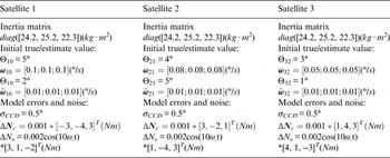
is the periodic component. The period angular velocity of the model error is ω° = 0.066°/s, and the sampling interval is set as Δt = 0.5s. In addition, it is assumed that the satellite formation consists of small satellites. The simulation parameters are given in Table 1.
Simulation parameters of the system.

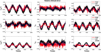
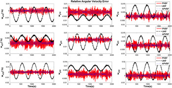
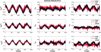
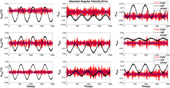
The simulation results are depicted in Figures 1–4, which show the relative/absolute attitude and angular velocity estimate errors. It is obvious that the estimate accuracy of the three filters is close to each other and has similar estimate trends in Figures 1 and 3. However, after careful review, it can be found that the APVSF has the best accuracy. Significant differences occur in the relative/absolute angular velocity estimate in Figures 2 and 4. The relative/absolute angular velocity estimates using UKF show obvious deviations and fluctuations. By contrast, the proposed APVSF and PVSF estimates are still bounded closely to a small region of the true state trajectory. It is evident that the proposed methods are more stable and robust than the UKF. The main reason behind this is that the proposed PVSF has the ability to update the model error; therefore, it can improve the system model precision, which plays an important role in enhancing the filtering performance. In addition, the estimate amplitude of APVSF is smaller than that of PVSF. This illustrates that the adaptive strategy to modify the PVSF has an obvious effect in improving estimate accuracy, which also shows its theoretical advantages and verifies the analyses in Section 4.
The estimation error of the relative attitude.

The estimation error of the relative angular velocity.

The estimation error of the absolute attitude.

The estimation error of the absolute angular velocity.

6. CONCLUSIONS
In this paper, the equations governing the attitude synchronisation estimation of the SFF are presented first. Then, the new estimate methodology referred to as the Predictive Variable Structure Filter (PVSF) is proposed; on which basis, the adaptive PVSF (APVSF) is further discussed based on the Mean-Square Error (MSE) principle. The (A)PVSF is a robust recursive corrector-predictor estimation method that can effectively deal with various types of model errors and measurement noise. In order to verify the performance of the proposed two methods, the numerical simulations are given to show that the PVSF and APVSF both have clear performance advantages over than that of the UKF for attitude synchronisation estimation. The APVSF has clearly better performance than PVSF, which demonstrates the effectiveness of the APVSF.
ACKNOWLEDGMENTS
This research work was supported by the National Natural Science Foundation of China (no. 61503414) and the State Key Laboratory of Astronautic Dynamics Foundation (ADL) (no. 2016ADL-DW0202). The authors will express their gratitude to the editors and reviewers for their valuable comments that helped to enhance the quality of this paper.
APPENDIX
In this subsection, the stability of the proposed PVSF will be proved. First of all, we define the measurement errors
 ${\bi e}_{y_{k + 1}} $
which may be calculated by using Equations (19) and (20), as follows:
 $$\eqalign{{\bi e}_{y_{k + 1}} & = {\bi y}_{k + 1} - \hat {\bi y}_{k + 1} \cr & = {\bi y}_{k + 1} - \hat {\bi y}_k - {\bi Z}\left[ {\hat {\bi x}}_k \right] - {\bi U}\left[ {\hat {\bi x}}_k \right]{\bi d}_k} $$
Substitution of Equations (22) and (23) into Equation (A1), and rearrangement of terms yields the following
 $$\eqalign{{\bi e}_{y_{k + 1}} & = {\bi e}_{y_{{{k + 1} / k}}} - \left( {\left \vert {{\bi e}_{y_{{{k + 1} / k}}}} \right \vert + \gamma \left \vert {{\bi e}_{y_k}} \right \vert} \right){\cdot} sign\left( {{\bi e}_{y_{{{k + 1} / k}}}} \right) \cr & = {\bi e}_{y_{{{k + 1} / k}}} - {\bi e}_{y_{{{k + 1} / k}}} - \gamma \left \vert {{\bi e}_{y_k}} \right \vert {\cdot} sign\left( {{\bi e}_{y_{{{k + 1} / k}}}} \right) \cr & = - \gamma \left \vert {{\bi e}_{y_k}} \right \vert {\cdot} sign\left( {{\bi e}_{y_{{{k + 1} / k}}}} \right)} $$
Let γ be a diagonal positive matrix such that γ ∈ ℝ m×m and with elements less than unity (i.e., 0 < γ ii < 1). By taking the absolute value of both sides of Equation (A2), the following is obtained
 $$\left \vert {{\bi e}_{y_{k + 1}}} \right \vert = \gamma \left \vert {{\bi e}_{y_k}} \right \vert \lt \left \vert {{\bi e}_{y_k}} \right \vert $$
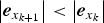
Therefore Equation (A3) proves that the measurement error decays with time. However, in order to prove the stability of the PVSF, we need to obtain the conclusion
 $\left\vert {{\bi e}_{x_{k + 1}}} \right\vert \lt \left\vert {{\bi e}_{x_k}} \right\vert$
from Equation (A3).
Based on the above discussion, we will prove the stability from the aspect of variable structure control. Let M k+1 used to form a Lyapunov function be defined by the absolute value of the measurement error, such that
 $$\eqalign{M_{k + 1} & = \left \vert {{\bi e}_{y_{k + 1}}} \right \vert \gt 0 \cr {\bi V} & = \displaystyle{1 \over 2}M_{k + 1}^2} $$
The estimation process is stable if the following is satisfied
 $$ \dot{\bi V} = M_{k + 1} \dot M_{k + 1} \lt 0$$
where
 $\dot M_{k + 1} $
is given by
 $$\dot M_{k + 1} = \left \vert {{\bi e}_{y_{k + 1}}} \right \vert - \left \vert {{\bi e}_{y_k}} \right \vert $$
Substitution of Equation (A6) into Equation (A5), and rearranging, yields the following
 $$\left \vert {{\bi e}_{y_{k + 1}}} \right \vert {\cdot} \left \vert {{\bi e}_{y_{k + 1}}} \right \vert \lt \left \vert {{\bi e}_{y_{k + 1}}} \right \vert {\cdot} \left \vert {{\bi e}_{y_k}} \right \vert $$
which is the stability condition for the PVSF and is equivalent to the following
 $$\left \vert {{\bi e}_{y_{k + 1}}} \right \vert \lt \left \vert {{\bi e}_{y_k}} \right \vert $$
To remove the absolute operator in Equation (A8), both sides are expressed in the form of diagonal matrices, and are multiplied by their respective transpose, as follows
 $$diag\left( {{\bi e}_{y_{k + 1}}} \right)diag\left( {{\bi e}_{y_{k + 1}}} \right)^T \lt\, diag\left( {{\bi e}_{y_k}} \right)diag\left( {{\bi e}_{y_k}} \right)^T $$
Assuming that the measurement function is well defined from Equation (11) and (12), the measurement error may be calculated as
 $${\bi e}_{y_{k + 1}} = {\bi h}\left( {{\bi x}_{k + 1}} \right) - {\bi h}\left( {\hat {\bi x}_{k + 1}} \right) + {\bi v}_{k + 1} \approx {\bi He}_{x_{k + 1}} + {\bi v}_{k + 1} $$
Substitution of Equation (A10) into Equation (A9) yields
 $$\eqalign{& \left( \matrix{diag\left( {{\bi He}_{x_{k + 1}}} \right)diag\left( {{\bi He}_{x_{k + 1}}} \right) + diag\left( {{\bi v}_{k + 1}} \right)diag\left( {{\bi v}_{k + 1}} \right) \hfill \cr +\, diag\left( {{\bi He}_{x_{k + 1}}} \right)diag\left( {{\bi v}_{k + 1}} \right) + diag\left( {{\bi v}_{k + 1}} \right)diag\left( {{\bi He}_{x_{k + 1}}} \right) \hfill} \right) \cr & \lt \left( \matrix{diag\left( {{\bi He}_{x_k}} \right)diag\left( {{\bi He}_{x_k}} \right) + diag\left( {{\bi v}_k} \right)diag\left( {{\bi v}_k} \right) \hfill \cr +\, diag\left( {{\bi He}_{x_k}} \right)diag\left( {{\bi v}_k} \right) + diag\left( {{\bi v}_k} \right)diag\left( {{\bi He}_{x_k}} \right) \hfill} \right)}$$
If the measurement noise is stationary white, then by taking the expected values of both sides in Equation (A11) and simplifying yields the following
 $$E\left[ \matrix{diag\left( {{\bi He}_{x_{k + 1}}} \right)diag\left( {{\bi He}_{x_{k + 1}}} \right) \hfill \cr +\, diag\left( {{\bi v}_{k + 1}} \right)diag\left( {{\bi v}_{k + 1}} \right) \hfill} \right] \lt E\left[ \matrix{diag\left( {{\bi He}_{x_k}} \right)diag\left( {{\bi He}_{x_k}} \right) \hfill \cr +\, diag\left( {{\bi v}_k} \right)diag\left( {{\bi v}_k} \right) \hfill} \right]$$
where
 $E\left[ {diag\left( {{\bi He}_{x_{k + 1}}} \right)diag\left( {{\bi v}_{k + 1}} \right)} \right]$
and
 $E\left[ {diag\left( {{\bi v}_{k + 1}} \right)diag\left( {{\bi He}_{x_{k + 1}}} \right)} \right]$
vanish due to the white noise assumption. For a diagonal, positive and time-invariant measurement matrix Equation (A12) becomes
 $$\eqalign{E\left[ {diag\left( {{\bi e}_{x_{k + 1}}} \right)diag\left( {{\bi e}_{x_{k + 1}}} \right)} \right] \lt E\left[ {diag\left( {{\bi e}_{x_k}} \right)diag\left( {{\bi e}_{x_k}} \right)} \right] \cr E\left( {\left \vert {{\bi e}_{x_{k + 1}}} \right \vert} \right) \lt E\left( {\left \vert {{\bi e}_{x_k}} \right \vert} \right)} $$
It is obvious that the condition Equation (A3) is satisfied, and the stable condition of the proposed PVSF Equation (A13) is also obtained. In other words, the stability of PVSF has been proved.
In addition, from Equations (19) to (21), we can obtain
 $${\bi e}_{y_{k + 1}} = {\bi y}_{k + 1} - \hat {\bi y}_{k + 1} = o\left( {\hat {\bi e}_{k + \Delta t}} \right)$$
Substitution of Equation (A14) into Equation (A8), yields the following
 $$\left \vert {o\left( {\hat {\bi e}_{k + \Delta t}} \right)} \right \vert \lt \left \vert {o\left( {\hat {\bi e}_k} \right)} \right \vert $$
It is obvious that the accuracy of the non-time Taylor expansion of Equation (19) will be enhanced with the convergence of state estimates gradually. In other words, the assumption of non-time Taylor expansion is reasonable and suitable for PVSF.