1 Introduction
The seminal work of Schubauer & Klebanoff (Reference Schubauer and Klebanoff1956), together with Emmons (Reference Emmons1951), laid the foundation of turbulent spot research for laminar-to-turbulent transition in the zero-pressure-gradient, smooth flat-plate boundary layer (ZPGSFPBL). In order to clarify the connection between any plausible momentary flow separation and the laminar layer breakdown, Schubauer & Klebanoff reported that:
Much time was spent in attempts to find evidence of momentary flow separation in transition regions. The most trustworthy method consisted of emitting iodine vapor from a small hole in the plate and noting by the discolouration of a starch film on the surface whether vapors ever traveled upstream. No evidence of separation could be found in any part of a transition region.
They further conjectured that:
While it is true that the velocity near the surface could reverse during part of a cycle when the amplitude [of the amplified disturbance wave] is high, this apparently is prevented by the action of the shearing stresses which become high at the same time.
The free-stream turbulence intensity level in their experiment ranges from  $0.02\,\%$ to
 $1\,\%$.
Although it is known that extremely rare backflow events can occur in a fully turbulent ZPGSFPBL (Johansson Reference Johansson1988), the Schubauer–Klebanoff conclusion regarding the total absence of negative skin friction in ZPGSFPBL transition has remained unchallenged over the past six decades. In hindsight, such a challenge should have occurred sooner than the present work. Here, we report our discovery of negative skin-friction events during the bypass transition in an extensively researched and representative ZPGSFPBL case, and in pipe flows with no-slip and slip boundary conditions, respectively. The peak probability of such events is located in the late stage of transition between the streamwise stations where the minimum and maximum mean skin friction are attained. The magnitude of the peak probability is substantially larger than the corresponding probability in the downstream fully turbulent region.
Boundary layers under an intermediate strength level of adverse pressure gradient may experience incipient detachment in which the probability of instantaneous backflow is less than  $1\,\%$. This was well established very early through a tremendous amount of work on separating flows over flat-plate and airfoil-type configurations (Simpson Reference Simpson1989; see also Wu & Squires Reference Wu and Squires1998), and it was traditionally thought that the subject of incipient detachment would stay within the realm of boundary layer separation under an adverse pressure gradient. Contrary to intuition, however, direct numerical simulation (DNS) data have provided solid evidence that very-low-level incipient detachment, weaker by two or three orders of magnitude compared to the
 $1\,\%$ threshold of Simpson (Reference Simpson1989), also occurs even in a fully turbulent ZPGSFPBL, in fully developed turbulent pipe flow and in fully developed turbulent channel flow (Hu, Morfey & Sandham Reference Hu, Morfey and Sandham2006; Lenaers et al. Reference Lenaers, Li, Brethouwer, Schlatter and Örlü2012; Khoury et al. Reference Khoury, Schlatter, Brethouwer and Johansson2014; Jalalabadi & Sung Reference Jalalabadi and Sung2018).
Given the engineering significance of skin friction during the laminar-to-turbulent transition of boundary layer and pipe flow, also considering the fundamental implication derived from the work of Schubauer & Klebanoff (Reference Schubauer and Klebanoff1956), one query arising naturally from the aforementioned recent confirmation of rare instantaneous negative skin friction in fully turbulent flows is whether the phenomenon of incipient detachment occurs during the laminar-to-turbulent transition in spatially developing ZPGSFPBLs, and in spatially developing pipe flows with no-slip and slip boundary conditions, respectively. Further, assuming it does occur, then how does the probability of incipient flow reversal during transition compare to the corresponding probability level in the downstream fully turbulent region? At what stage of transition (early transition, breakdown or near the completion of transition) does the probability of incipient flow reversal reach its maximum level? How do the number density, the wall-normal extent and the wall footprint size/shape of incipient flow reversal during transition compare to those in the downstream fully turbulent region? From a mechanism point of view, what is the underlying vortex structure associated with the incipient flow reversal during transition? In this article, we address these questions.
We begin by briefly reviewing the progress made over the past two decades on detecting incipient detachment in fully turbulent ZPGSFPBLs and in fully developed turbulent pipe flows.
The first plausible indication of incipient flow reversal in fully turbulent ZPGSFPBL was found by Johansson (Reference Johansson1988) from measurements with the laser Doppler velocimetry (LDV) technique. This was followed by the report of near-wall backflow in a complex turbulent boundary layer from the DNS work of Spalart & Coleman (Reference Spalart and Coleman1997). Owing to the issue of the inaccurate inflow turbulence generation method, as commonly encountered in the early DNS studies of external flows, the upstream turbulent inflow of Spalart & Coleman does not possess the Reynolds shear stress properties of a canonical turbulent ZPGSFPBL. The pioneering work of Johansson (Reference Johansson1988) and Spalart & Coleman (Reference Spalart and Coleman1997) suggested the plausible existence of incipient flow reversal in fully turbulent ZPGSFPBLs, but, given the limitations of the early LDV technology and of the spatially developing DNS methodology as of two decades ago, their quantitative instantaneous backflow data should perhaps be viewed with caution.
The advances in spatially developing boundary layer DNS that occurred 10 years ago (Schlatter et al. Reference Schlatter, Örlü, Li, Brethouwer, Fransson, Alfredsson and Henningson2009; Wu & Moin Reference Wu and Moin2009) made it possible to examine the plausible incipient detachment in fully turbulent ZPGSFPBLs with high precision. Lenaers et al. (Reference Lenaers, Li, Brethouwer, Schlatter and Örlü2012) analysed the fully turbulent ZPGSFPBL data of Schlatter & Örlü (Reference Schlatter and Örlü2010). The probability of instantaneous negative skin friction in their turbulent ZPGSFPBL was found to be  $0.08\,\%$ at
 $Re_{\unicode[STIX]{x1D70F}}=u_{\unicode[STIX]{x1D70F}}\unicode[STIX]{x1D6FF}/\unicode[STIX]{x1D708}=1000$, where
 $u_{\unicode[STIX]{x1D70F}}$ is the friction velocity,
 $\unicode[STIX]{x1D708}$ is the kinematic viscosity and
 $\unicode[STIX]{x1D6FF}$ is the boundary layer thickness. The wall-normal extent of the backflow region is within the first
 $8.5$ wall units. The shape of the incipient backflow is approximately circular, with an average diameter approximately 20 viscous units independent of Reynolds number. Lenaers et al. (Reference Lenaers, Li, Brethouwer, Schlatter and Örlü2012) suggested that the backflow is located inside a low-speed streak, which is in turn caused by a strong oblique vortex arising from streak instability.
Aside from the pipe flow and the ZPGSFPBL, instantaneous backflow was discovered in fully developed turbulent channel flow by Hu et al. (Reference Hu, Morfey and Sandham2006). Cardesa et al. (Reference Cardesa, Monty, Soria and Chong2014) investigated the critical point (position with zero wall stress vector) in turbulent channel flow at  $Re_{\unicode[STIX]{x1D70F}}=934$ and
 $1843$. They found that the average lifetime of the critical points is short at approximately
 $6.6$ viscous time units
 $\unicode[STIX]{x1D708}/u_{\unicode[STIX]{x1D70F}}^{2}$. They also reported that critical points exist at the tail (upstream end) of a large-scale structure that extends from the wall to the outer edge of the logarithmic region, and an incipient flow reversal region extends over
 $800$ wall units downstream of the critical points. This last point is not supported by the channel flow analysis of Lenaers et al. (Reference Lenaers, Li, Brethouwer, Schlatter and Örlü2012).
Brücker (Reference Brücker2015) presented solid experimental evidence confirming the near-wall instantaneous backflow in a turbulent ZPGSFPBL by means of imaging two-dimensional arrays of flexible micropillars attached to the wall. The measurements were performed at  $Re_{\unicode[STIX]{x1D70F}}=940$, similar to the Reynolds numbers considered in the turbulent ZPGSFPBL of Lenaers et al. (Reference Lenaers, Li, Brethouwer, Schlatter and Örlü2012) and in the turbulent channel flow of Cardesa et al. (Reference Cardesa, Monty, Soria and Chong2014). In the DNS of Schlatter & Örlü (Reference Schlatter and Örlü2010), the momentum-thickness Reynolds number
 $Re_{\unicode[STIX]{x1D703}}$ corresponding to
 $Re_{\unicode[STIX]{x1D70F}}=940$ is approximately
 $2800$, and they showed that the flow statistics at this Reynolds number conform to those of a canonical turbulent ZPGSFPBL. Brücker (Reference Brücker2015) deduced the wall shear stress vector by measuring the bending of the micropillars. Near-wall backflow regions are often found in areas with high spanwise gradients of the wall shear stress, and incipient flow reversal is therefore considered by Brücker to be the result of strong curvature of the near-wall flow around the critical point.
Willert et al. (Reference Willert, Cuvier, Foucaut, Klinner, Stanislas, Laval, Srinath, Soria, Amili and Atkinson2018) reported an extensive experimental study on incipient backflow in a fully turbulent ZPGSFPBL over a wide range of Reynolds numbers  $(2500<Re_{\unicode[STIX]{x1D703}}<8000)$. Their high-magnification particle image velocimetry (PIV) captured the rare reverse flow events, and time-resolved PIV was used in the statistical sampling. The probability of negative skin friction was found to be of the order of
 $0.012\,\%$ to
 $0.018\,\%$, slightly lower than that in the DNS of Lenaers et al. (Reference Lenaers, Li, Brethouwer, Schlatter and Örlü2012) but still of the same order of magnitude. They found that a typical incipient detachment bubble is approximately
 $30$ wall units in length and
 $5$ wall units in height, in agreement with Lenaers et al. (Reference Lenaers, Li, Brethouwer, Schlatter and Örlü2012).
In their studies of fully developed turbulent pipe flow, Khoury et al. (Reference Khoury, Schlatter, Brethouwer and Johansson2014) mentioned in passing the existence of negative skin friction. Their probability density function (p.d.f.) of wall shear stress at  $Re_{\unicode[STIX]{x1D70F}}=u_{\unicode[STIX]{x1D70F}}R/\unicode[STIX]{x1D708}=1000$ (where
 $R$ is the pipe radius) agrees well with that of the turbulent boundary layer of Lenaers et al. (Reference Lenaers, Li, Brethouwer, Schlatter and Örlü2012) at similar Reynolds number. Incipient detachment was found to occur more frequently with increasing Reynolds number from
 $Re_{\unicode[STIX]{x1D70F}}=180$ to
 $1000$. Jalalabadi & Sung (Reference Jalalabadi and Sung2018) reported a more comprehensive DNS study on the issue of incipient detachment in fully developed turbulent pipe flow at
 $Re_{\unicode[STIX]{x1D70F}}=544$. Instantaneous backflow was found to be a rare event with a probability less than
 $0.1\,\%$, and the backflow extends up to
 $4$ wall units from the pipe surface. They further examined the flow features around the backflow using conditional averaging. The wall footprint of the averaged incipient detachment region has an irregular polygon shape, with a spanwise dimension of
 $30$ wall units and a streamwise dimension of
 $15$ wall units, respectively. This is in broad agreement with Lenaers et al. (Reference Lenaers, Li, Brethouwer, Schlatter and Örlü2012). Jalalabadi & Sung (Reference Jalalabadi and Sung2018) considered that the cause of the backflow is the presence of a spanwise vortex in the buffer layer, which differs to a certain degree from the argument of Lenaers et al. (Reference Lenaers, Li, Brethouwer, Schlatter and Örlü2012) that the incipient near-wall backflow resides in a low-speed streak generated by an oblique vortex.
Chin et al. (Reference Chin, Monty, Chong and Marusic2018) studied critical points in fully developed turbulent pipe flow at  $Re_{\unicode[STIX]{x1D70F}}=1000$. Their conditionally averaged streamwise wall shear stress contours display a roughly circular region of negative values surrounding a critical point pair – this aspect is confirmed in the present study. Slightly downstream of the circular area is an elongated region with weaker values of negative streamwise wall shear stress. Similar to the channel flow results of Cardesa et al. (Reference Cardesa, Monty, Soria and Chong2014) and Brücker (Reference Brücker2015), the spanwise wall shear stress displays strong variations both upstream and downstream of the critical point pair. Chin et al. (Reference Chin, Monty, Chong and Marusic2018) also showed that the conditionally averaged vortex field surrounding a pair of critical points contains two hairpin vortices: a downstream reverse hairpin vortex, whose head element is directed towards the wall, and an upstream normal hairpin vortex.
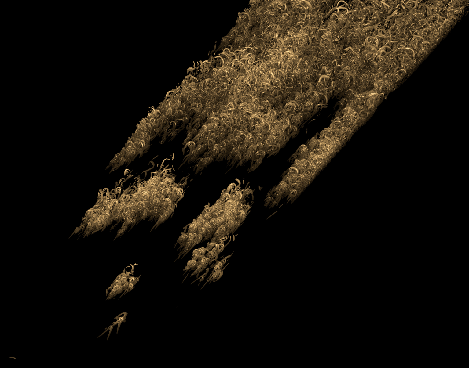
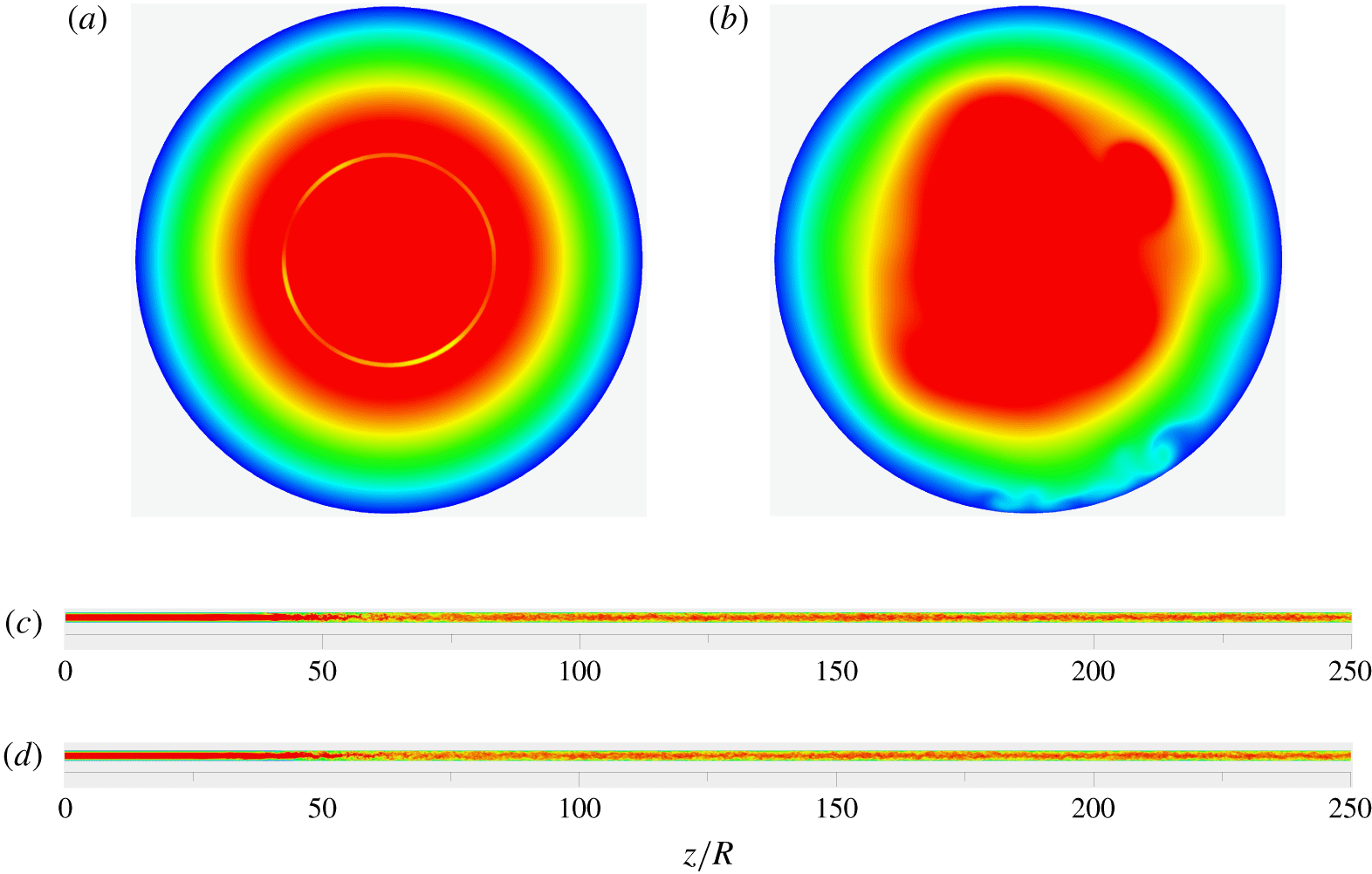
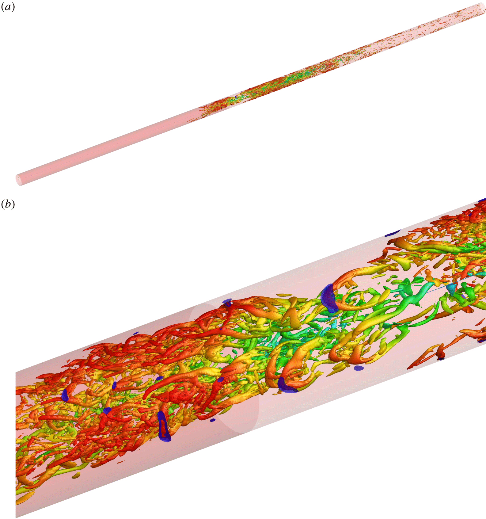
It is thus evident that the phenomenon of extremely rare incipient detachment events has been firmly established for fully developed turbulent pipe flow and fully turbulent ZPGSFPBL. Guided by the understanding developed by previous researchers on the incipient detachment in fully turbulent flows as cited above, here we consider questions related to incipient detachment during the laminar-to-turbulent transition processes in a spatially developing ZPGSFPBL (figure 1) and in pipe flows with slip and no-slip boundary conditions (figure 2), respectively. Our flow simulations start from a semi-analytical laminar inlet state, going through a well-controlled bypass transition process, and arrive at a fully turbulent state.
Visualization of the transitional and turbulent ZPGSFPBL (case 1) using the instantaneous isosurface of swirling strength  $\unicode[STIX]{x1D706}_{ci}=22\times 5.33\times 10^{-4}\,U_{f}/\unicode[STIX]{x1D703}_{0}$ over the region
 $200<Re<700$ at the instant
 $t=98\,300\,\unicode[STIX]{x0394}t$. The colour scheme corresponds to the isosurface’s wall-normal position
 $y/\unicode[STIX]{x1D6FF}$ with the white colour indicating
 $y/\unicode[STIX]{x1D6FF}\geqslant 1$.

Visualization of the transitional and turbulent pipe flow using instantaneous contours of axial velocity  $u_{z}/V$: (a) over the inlet plane in case 2 (no slip) and in case 3 (slip); (b) over the
 $z/R=30$ plane in case 3; (c) over the
 $\unicode[STIX]{x1D703}=0$ and
 $180^{\circ }$ planes in case 2; (d) over the
 $\unicode[STIX]{x1D703}=0$ and
 $180^{\circ }$ planes in case 3. The red colour indicates
 $u_{z}/V\geqslant 1.4$, whereas deep blue corresponds to
 $u_{z}/V=0$.

It turns out not only that incipient detachment does exist during the processes of laminar-to-turbulent transition of spatially developing ZPGSFPBL and pipe flows, but also that its peak probability of occurrence can actually reach (in pipe flow) as high as two orders of magnitude larger than those previously found in the fully turbulent region; the normalized wall-normal extent of the incipient detachment region during transition is also larger than that in the downstream fully turbulent region. This suggests that instantaneous near-wall backflow during transition is a statistically notable phenomenon that should not be disregarded on the grounds of presumed extremely low probability. Statistics on the number density and the area of negative skin-friction patches are acquired, together with the conditionally averaged wall shear stress field surrounding the geometric centre of the negative skin-friction patch. On average, the shape of the negative skin-friction region is small and nearly circular, in broad agreement with Lenaers et al. (Reference Lenaers, Li, Brethouwer, Schlatter and Örlü2012) and Jalalabadi & Sung (Reference Jalalabadi and Sung2018); this is also in partial agreement with Chin et al. (Reference Chin, Monty, Chong and Marusic2018) but without their downstream wake containing additional mild negative skin friction. The conditionally averaged wall shear stress field displays a pair of critical points, one in the fore and the other in the aft of the nearly circular negative skin-friction patch. Similar to Cardesa et al. (Reference Cardesa, Monty, Soria and Chong2014) and Brücker (Reference Brücker2015), strong spanwise variation of the wall shear stress field is detected near the negative skin-friction patch. Many of the kinematic statistics on the backflow events in the fully turbulent regions from the present study agree with previous data, which reinforces confidence in the reliability of the present findings in the transitional region.
For both the boundary layer and pipe flows considered here, and in both the transitional and fully turbulent regions, the incipient negative skin friction is found, through instantaneous flow visualization and conditional averaging, to be induced by the head element of a reverse hairpin vortex. This finding is different from the recent report by Chin et al. (Reference Chin, Monty, Chong and Marusic2018) that, in fully developed turbulent pipe flow, incipient negative skin friction is caused by a pair of forward and reverse hairpin vortices. The finding of Jalalabadi & Sung (Reference Jalalabadi and Sung2018) that the negative skin friction is due to a buffer layer spanwise vortex element is consistent with the current more complete picture – their buffer layer spanwise vortex being the head element of the reverse hairpin vortex. This picture does not involve the scenario of critical points being located either at the tail (upstream end) of some large-scale structure (Cardesa et al. Reference Cardesa, Monty, Soria and Chong2014) or inside a low-speed streak (Lenaers et al. Reference Lenaers, Li, Brethouwer, Schlatter and Örlü2012).
2 Flow cases considered
A total of four DNS were performed to study the plausible incipient detachment in transition. The first flow we use is an incompressible ZPGSFPBL developing spatially beneath a continuous flow of free-stream isotropic turbulence, from an initial laminar state, through a well-controlled process of bypass transition in the narrow sense (figure 1), as defined in Wu et al. (Reference Wu, Moin, Wallace, Skarda, Adrián and Hickey2017), to the canonical fully turbulent state. This boundary layer DNS (case 1) was performed on a mesh with  $16\,384\times 500\times 512$ grid points in the streamwise, wall-normal and spanwise directions, respectively. The domain size is
 $21\,563\unicode[STIX]{x1D703}_{0}\times 2250\unicode[STIX]{x1D703}_{0}\times 844\unicode[STIX]{x1D703}_{0}$, where
 $\unicode[STIX]{x1D703}_{0}$ is the inlet momentum thickness. The momentum-thickness Reynolds number
 $Re_{\unicode[STIX]{x1D703}}$ develops from
 $80$ to
 $3000$, with the growth of
 $\unicode[STIX]{x1D6FF}$ from
 $7.55\unicode[STIX]{x1D703}_{0}$ to
 $312\unicode[STIX]{x1D703}_{0}$. The
 $Re_{\unicode[STIX]{x1D70F}}$ value reaches 1003 at the exit. In the transitional region of
 $80<Re_{\unicode[STIX]{x1D703}}<800$, the present DNS grid resolutions on wall-parallel planes are
 $3.5<\unicode[STIX]{x0394}x^{+}<5.5$ and
 $4.5<\unicode[STIX]{x0394}z^{+}<7$, respectively, where the superscript
 $+$ denotes normalization with viscous scales. In the turbulent region of
 $800<Re_{\unicode[STIX]{x1D703}}<3000$, the grid resolutions are
 $4.3<\unicode[STIX]{x0394}x^{+}<5$ and
 $5.3<\unicode[STIX]{x0394}z^{+}<6.1$, respectively. Measured using local values of the Kolmogorov length scale
 $\unicode[STIX]{x1D702}=(\unicode[STIX]{x1D708}^{3}/\unicode[STIX]{x1D700})^{1/4}$, at the station
 $Re_{\unicode[STIX]{x1D703}}=2900$, the streamwise grid resolution is
 $2<\unicode[STIX]{x0394}x/\unicode[STIX]{x1D702}<3$ for the inner layer, and
 $0.5<\unicode[STIX]{x0394}x/\unicode[STIX]{x1D702}<2$ in the outer region. Along the wall-normal direction the resolution is
 $0.4<\unicode[STIX]{x0394}y/\unicode[STIX]{x1D702}<2$ throughout the boundary layer. The inlet free-stream turbulence generation approach adopted here belongs to the category of strong recycling method of inflow turbulence generation (Wu Reference Wu2017). The time step of the DNS is
 $\unicode[STIX]{x0394}t=1.125\unicode[STIX]{x1D703}_{0}/U_{f}$, where the subscript
 $f$ refers to constant mean free-stream value. Although not shown here, an extensive validation study was also performed by comparing the present DNS mean and second-order turbulent statistics with the experimental data of DeGraaff & Eaton (Reference DeGraaff and Eaton2000) at
 $Re_{\unicode[STIX]{x1D703}}=2900$, and with the DNS of Schlatter & Örlü (Reference Schlatter and Örlü2010) at
 $Re_{\unicode[STIX]{x1D703}}=2536$. Furthermore, our DNS profiles for the rate of viscous dissipation of turbulent kinetic energy
 $\unicode[STIX]{x1D700}^{+}=\unicode[STIX]{x1D700}/(u_{\unicode[STIX]{x1D70F}}^{4}/\unicode[STIX]{x1D708})$ as a function of
 $y^{+}$ are in excellent agreement, not only in slope but also in intercept, over the logarithmic region, with the asymptotic theoretical relation
 $\unicode[STIX]{x1D700}^{+}=1/(\unicode[STIX]{x1D705}y^{+})$. Further details about the ZPGSFPBL simulation can be found in Wu, Wallace & Hickey (Reference Wu, Wallace and Hickey2019).
Because of the sensitivity of skin friction during transition to inflow and free-stream conditions, in order to achieve generality, it is important to ensure that the flows to be investigated are canonical and representative. Indeed, case 1 is such a canonical flow. In fact, it is nearly identical to the ERCOFTAC T3A case (Roach & Brierley Reference Roach and Brierley1992) with an inlet Blasius laminar boundary layer beneath  $3\,\%$ initial intensity of free-stream homogeneous isotropic turbulence (the integral length scale may differ). This particular flow case has been extensively used as a benchmark test case in bypass transition modelling (see Durbin (Reference Durbin2012) and Wei et al. (Reference Wei, Ge, George and Durbin2017) and many others) and it has also been used extensively in DNS studies on bypass transition mechanism (see Jacobs & Durbin (Reference Jacobs and Durbin2001) and Brandt, Schlatter & Henningson (Reference Brandt, Schlatter and Henningson2004) and many others). As such, the results acquired from the present study on case 1 are expected to carry generality within the category of boundary layer bypass transition in the narrow sense.
The second and third cases we study in this work are the spatially developing pipe flows starting from a laminar inflow state, through transition, to the fully developed turbulent state with no-slip (case 2) and slip (case 3) boundary conditions, respectively. The governing equations are the continuity and three-dimensional Navier–Stokes equations for incompressible flow in cylindrical coordinates. The fractional step method computer program and the details of the numerical scheme were described by Pierce & Moin (Reference Pierce and Moin2001, Reference Pierce and Moin2004) in their large-eddy simulation of combustion in a coaxial jet combustor. The inlet base flow in the pipe simulations has a fully developed parabolic laminar velocity profile, except for that inside a narrow numerical ring of  $0.4\leqslant r/R\leqslant 0.42$ (figure 2a), where
 $r$ is the radial coordinate. Within the numerical ring of the inlet plane, the exact laminar parabolic velocity profile is replaced by time-dependent, fully developed turbulent pipe flow DNS velocity fields through a random permutation and concatenation procedure (Wu Reference Wu2017). The introduced inlet disturbances mimic, to some extent, the turbulent wake behind a thin wire ring, which is of circumferential mode in nature. The mass flow rate over the inlet plane is kept constant with time. In the present pipe DNS,
 $Re=VD/\unicode[STIX]{x1D708}=8000$, where
 $D$ is the pipe diameter,
 $V$ is the bulk velocity and the pipe length is
 $250R$ (figure 2c,d). The computational mesh size is
 $8192\times 200\times 256$ in the axial, radial and azimuthal directions, respectively. In the late transitional region and in the fully developed turbulent region of case 2, the axial resolution
 $\unicode[STIX]{x0394}z$ is less than
 $4.5\unicode[STIX]{x1D702}$ and the radial resolution
 $\unicode[STIX]{x0394}r$ is always less than
 $1.0\unicode[STIX]{x1D702}$. Further details about the case 2 DNS can be found in Wu et al. (Reference Wu, Moin, Adrian and Baltzer2015).
The case 2 configuration corresponds to the most fundamental and the simplest internal flow, namely, smooth pipe flow with fully developed laminar inlet condition. Many landmark fundamental pipe transition studies have been performed by previous researchers in such a configuration superimposed with different types of inlet finite-amplitude perturbations. Wygnanski & Champagne (Reference Wygnanski and Champagne1973) produced their perturbations by placing a cylinder, orifice or disk near the inlet. Hof et al. (Reference Hof, Westerweel, Schneider and Eckhardt2006) and Avila et al. (Reference Avila, Moxey, Lozar, Avila, Barkley and Hof2011) issued impulsive jets through small holes on their pipe wall. All these studies produced results that are considered to be generally applicable to the fundamental problem of pipe transition. Here, we adopt the same philosophy. As stated, in case 2, we used a narrow numerical ring to produce the inlet disturbance. We also performed simulations by moving the numerical ring to a different location; those simulations also result in qualitatively the same type of negative skin-friction peak during transition. Of course, the quantitative peak levels vary with the imposed perturbations, but the trends remain the same. More importantly, the negative skin-friction peak during transition is found in both pipe flow and ZPGSFPBL.
In case 3, the slip boundary condition is applied on the pipe wall following the approach of Min & Kim (Reference Min and Kim2004) in their DNS on fully developed turbulent channel flow:
 $$\begin{eqnarray}u_{z,wall}=-L_{z}\left.\frac{\unicode[STIX]{x2202}u_{z}}{\unicode[STIX]{x2202}r}\right|_{wall},\quad u_{r,wall}=0,\quad u_{\unicode[STIX]{x1D703},wall}=0,\end{eqnarray}$$
where  $u_{z}$,
 $u_{r}$ and
 $u_{\unicode[STIX]{x1D703}}$ are the instantaneous velocity components in the axial, radial and circumferential directions, respectively. Numerical stiffness is incurred in this third DNS case due to the fact that the axial velocity at the wall depends upon the local instantaneous velocity gradient. As a result, in order to maintain numerical stability, the time step in case 3 is reduced by a factor of 8 to
 $\unicode[STIX]{x0394}t=0.001R/V$ from the original
 $\unicode[STIX]{x0394}t=0.008R/V$ in case 2, which substantially increased the cost of the DNS. The Courant–Friedrichs–Lewy (CFL) number is always less than 0.08 in case 3. Owing to the substantially increased computational cost, the slip length is set as a single constant
 $L_{z}=0.005R$, chosen from the range of values considered by Min & Kim (Reference Min and Kim2004) and Jung, Choi & Kim (Reference Jung, Choi and Kim2016).
Case 4 is an auxiliary simulation on the fully developed turbulent pipe flow at  $Re=VD/\unicode[STIX]{x1D708}=8000$ using the conventional axially periodic boundary condition over a
 $30R$ long domain with a grid
 $2048\times 256\times 512$. This auxiliary DNS case is used as a benchmark to check the consistency of the turbulent statistics extracted from the spatially developing pipe simulations (case 2) in the fully developed turbulent region downstream of transition.
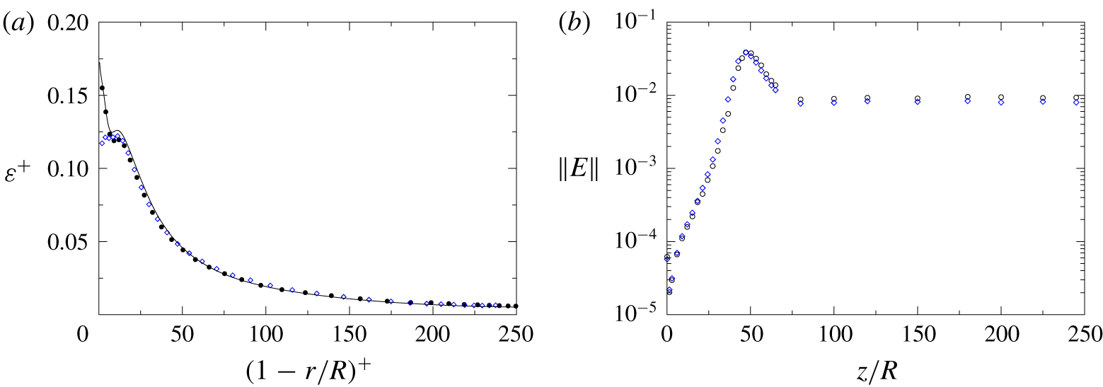
Figure 3(a) shows the radial profiles of  $\unicode[STIX]{x1D700}^{+}=\langle \unicode[STIX]{x1D700}\rangle /(u_{\unicode[STIX]{x1D70F}}^{4}/\unicode[STIX]{x1D708})$ as a function of
 $(1-r/R)^{+}$ sampled over the region
 $200<z/R<230R$ in case 2 and in case 3, together with the benchmark profile from the auxiliary case 4. In this paper,
 $\langle \cdot \rangle$ implies averaging over the homogeneous direction and over time. In figure 3(a), the three sets of results agree closely except for the region of
 $(1-r/R)^{+}<10$. Within the first 10 wall units, the no-slip pipe flow profiles (case 2 and case 4) exhibit the well-known shoulder followed by a sharp increase towards the wall, whereas the slip case 3 profile displays a double-peak pattern. In figure 3(b) the axial cross-sectional integrated energy norm
 $\Vert E(z)\Vert =\int _{0}^{R}(u_{z,rms}^{\prime 2}+u_{\unicode[STIX]{x1D703},rms}^{\prime 2}+u_{r,rms}^{\prime 2})r\,\text{d}r/(R^{2}V^{2})$ is plotted as a function of the axial distance
 $z/R$. It is seen from the figure that the slip case 3 data are in close agreement with those of the no-slip case 2 during transition, indicating similar rates of disturbance amplification with distance. The peaks of the energy norm in both cases are located at
 $z\approx 50R$, close to the locations of the maximum mean friction factor. Thus, it is likely that the transition process is not substantially modified by the slip boundary condition under the prescribed inflow condition (figure 2a) and the prescribed slip length. Figure 3(b) also shows that downstream of the peak location for
 $50R<z<250R$, the profile of
 $\Vert E(z)\Vert$ extracted from case 3 remains a constant and below that of the no-slip case 2, consistent with the fact that the turbulence level is reduced as a result of weakened near-wall shear in the slip case 3. At the prescribed slip-length value
 $L_{z}=0.005R$, the effect of the slip boundary condition on turbulent pipe flow statistics is weak after normalization by inner variables. This observation is consistent with the findings reported by Bae et al. (Reference Bae, Lozano-Durán, Bose and Moin2019) in fully developed turbulent channel flows with slip boundary conditions.
Rate of dissipation and norm of the turbulent kinetic energy in the pipe flows at  $Re_{D}=8000$. (a) Radial profiles of
 $\unicode[STIX]{x1D700}^{+}=\langle \unicode[STIX]{x1D700}\rangle /(u_{\unicode[STIX]{x1D70F}}^{4}/\unicode[STIX]{x1D708})$: filled circles, case 2 (no-slip) sampled over
 $220<z/R<230$; open diamonds, case 3 (slip) sampled over
 $220<z/R<230$; full line, case 4 (axially periodic simulation of fully developed no-slip turbulent pipe flow). (b) Axial profiles of
 $\Vert E\Vert =\int _{0}^{R}(u_{z,rms}^{\prime 2}+u_{\unicode[STIX]{x1D703},rms}^{\prime 2}+u_{r,rms}^{\prime 2})r\,\text{d}r/(R^{2}V^{2})$; open circles, case 2; open diamonds, case 3.

3 Probability of negative skin friction
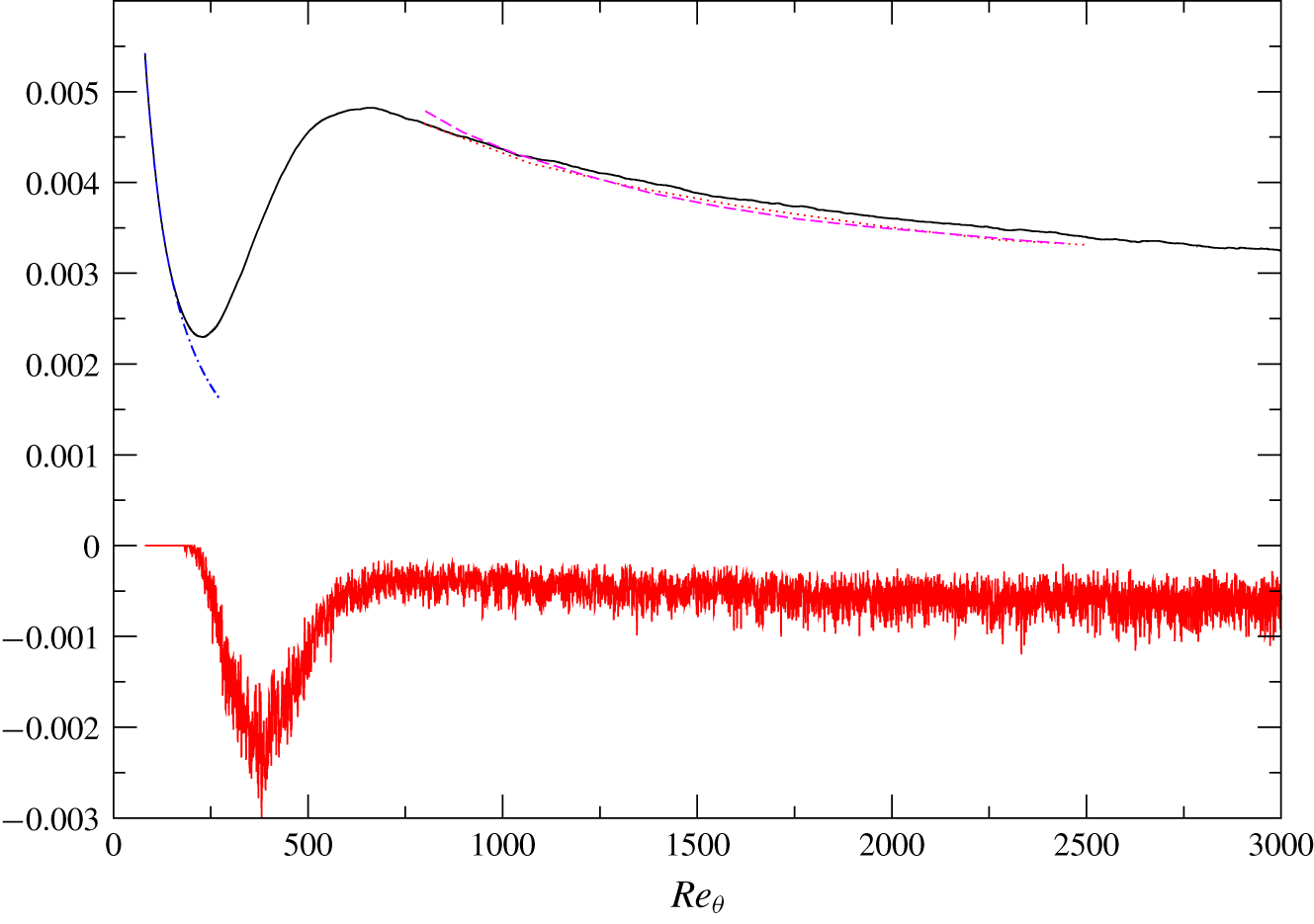
The mean skin-friction coefficient  $\langle C_{f}\rangle$ from case 1 is compared in figure 4 with the Blasius solution prior to the breakdown of the laminar boundary layer, and with the fully turbulent DNS data of Schlatter & Örlü (Reference Schlatter and Örlü2010) and Lee & Sung (Reference Lee and Sung2011) after the completion of transition. The excellent collapse of
 $C_{f}$ onto the Blasius solution is particular noteworthy, as it offers a piece of strong proof that the present ZPGSFPBL goes through a well-controlled and clean process of bypass transition in the narrow sense. In the fully turbulent region after transition, the present
 $\langle C_{f}\rangle$ is in good agreement with, but slightly higher than, those of Schlatter & Örlü (Reference Schlatter and Örlü2010) and Lee & Sung (Reference Lee and Sung2011). This is most likely due to the facts that our boundary layer is developing from laminar through transition to turbulent state, and is with a decaying free-stream turbulence whose inlet intensity is
 $3\,\%$.
Mean skin-friction coefficient  $\langle C_{f}\rangle$ (upper set of curves) and the probability of negative instantaneous skin friction
 $C_{f}<0$ (lower curve, multiplied by
 $-1$) in the transitional and turbulent ZPGSFPBLs (case 1) as a function of
 $Re_{\unicode[STIX]{x1D703}}$. The probability is defined as the ratio of the surface area with negative skin friction to the total surface area. Solid lines, present DNS; dashed line, Schlatter & Örlü (Reference Schlatter and Örlü2010); dotted line, Lee & Sung (Reference Lee and Sung2011); dot-dashed line, Blasius solution.

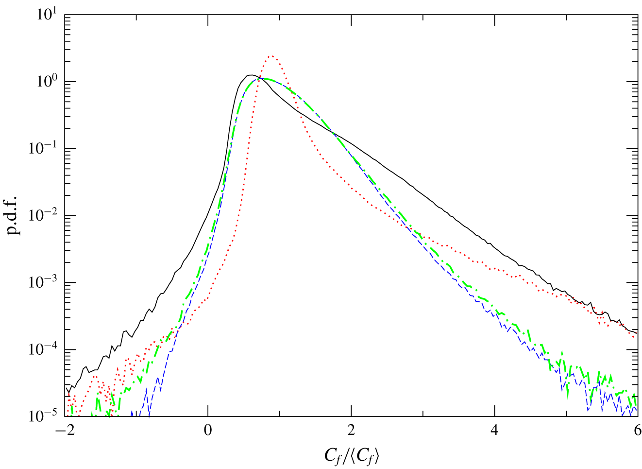
The p.d.f. of normalized instantaneous skin-friction coefficient  $C_{f}/\langle C_{f}\rangle$ in the transitional and turbulent ZPGSFPBLs (case 1). Dotted line, transitional region
 $220<Re<240$, where
 $\langle C_{f}\rangle$ reaches its minimum; solid line, transitional region
 $370<Re<390$, where the probability of negative
 $C_{f}$ reaches its maximum; dashed line, low-Reynolds-number turbulent region
 $990<Re<1010$; dot-dashed line, fully turbulent region
 $2790<Re<2810$.

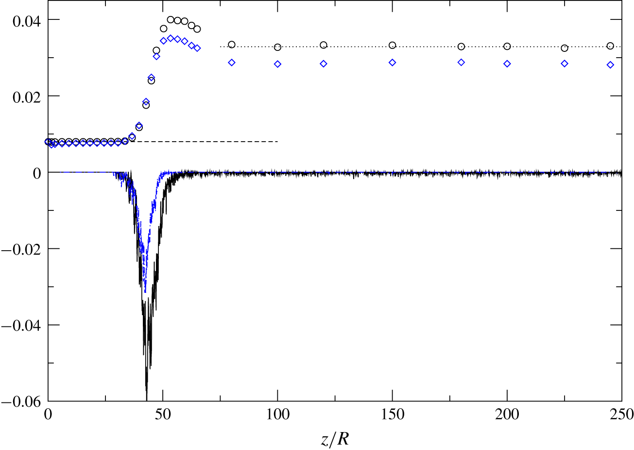
Mean friction factor  $\langle f\rangle$ (upper set) and the probability of negative instantaneous friction factor
 $f<0$ (lower set of curves, multiplied by
 $-1$) as a function of
 $z/R$ in the spatially developing transitional and turbulent pipe flows at
 $Re_{D}=8000$. The probability is defined as the ratio of surface area with
 $f<0$ to the total surface area. Open circles and solid line, case 2 (no-slip); diamonds and dot-dashed line, case 3 (slip); dashed line,
 $f=64/Re_{D}$ for fully developed laminar pipe flow; dotted line, Moody’s correlation for fully developed turbulent pipe flow.

The probability of negative instantaneous skin friction as a function of the momentum-thickness Reynolds number for the ZPGSFPBL is also given in figure 4. The probability stays at zero during the early stage of transition, namely, from the inlet  $(Re_{\unicode[STIX]{x1D703}}\approx 80)$ to the onset of breakdown of the laminar boundary layer where the precursor of an infant turbulent spot, in the form of a
 $\unicode[STIX]{x039B}$ vortex structure, starts to occur (figure 1). In other words, during the stage of initial amplification of the instability in boundary layer bypass transition in the narrow sense, there is virtually no occurrence of instantaneous negative skin friction. The statistical location of the onset of the laminar layer breakdown is indicated, in the upper set of curves of figure 4, by the departure of the mean skin-friction coefficient
 $\langle C_{f}\rangle$ from the Blasius solution at
 $Re_{\unicode[STIX]{x1D703}}\approx 200$. This location is adjacent to the minimum
 $\langle C_{f}\rangle$ location at
 $Re_{\unicode[STIX]{x1D703}}\approx 230$, which we consider as the location for the end of the early transition stage. The
 $\unicode[STIX]{x039B}$ vortex structures have evolved into chaotic infant turbulent spots by the completion of the early transition stage. The location of the maximum mean skin friction
 $\langle C_{f}\rangle$ at
 $Re_{\unicode[STIX]{x1D703}}\approx 670$ is statistically near the end of the boundary layer transition where mature transitional–turbulent spots have merged into a seemingly continuous flow of turbulence. Figure 4 indicates that the maximum probability of negative skin friction,
 $0.3\,\%$, is found at
 $Re_{\unicode[STIX]{x1D703}}\approx 380$, between the breakdown and the completion of transition. At this location,
 $Re_{\unicode[STIX]{x1D703}}\approx 380$, the mean skin friction
 $\langle C_{f}\rangle$ has a steep slope with respect to
 $Re_{\unicode[STIX]{x1D703}}$, and the turbulent/non-turbulent intermittency is strong. Over the wide transitional range of
 $200<Re_{\unicode[STIX]{x1D703}}<700$, the zonal-averaged probability of
 $C_{f}<0$ is
 $0.11\,\%$. Further downstream, for the low-Reynolds-number turbulent range
 $800<Re_{\unicode[STIX]{x1D703}}<1200$ and the (relatively) high-Reynolds-number turbulent range
 $2400<Re_{\unicode[STIX]{x1D703}}<2800$, the zonal-averaged probabilities of
 $C_{f}<0$ are
 $0.04\,\%$ and
 $0.06\,\%$, respectively. These turbulent zonal-averaged results are in reasonably good agreement with the two published turbulent ZPGSFPBL data points, namely,
 $0.06\,\%$ from Lenaers et al. (Reference Lenaers, Li, Brethouwer, Schlatter and Örlü2012) and
 $0.012\,\%{-}0.018\,\%$ from Willert et al. (Reference Willert, Cuvier, Foucaut, Klinner, Stanislas, Laval, Srinath, Soria, Amili and Atkinson2018). The slight increase, from
 $0.04\,\%$ to
 $0.06\,\%$, with Reynolds number is also consistent with the observation of Lenaers et al. (Reference Lenaers, Li, Brethouwer, Schlatter and Örlü2012). Note that these turbulent ZPGSFPBL data points are substantially less than the peak probability of
 $0.3\,\%$ and the zonal-averaged probability of
 $0.11\,\%$ attained during the process of boundary layer transition.
The p.d.f. profiles of the normalized instantaneous skin-friction coefficient  $C_{f}/\langle C_{f}\rangle$ over four selected streamwise regions of the boundary layer are shown in figure 5. The two selected transitional regions are
 $220<Re_{\unicode[STIX]{x1D703}}<240$ where the minimum
 $\langle C_{f}\rangle$ is attained, and
 $370<Re_{\unicode[STIX]{x1D703}}<390$ over which the probability of negative
 $C_{f}$ reaches its maximum, respectively. The former has a more narrowband characteristic with a sharp high peak reached at
 $C_{f}/\langle C_{f}\rangle =0.85$, implying that instantaneous
 $C_{f}$ has relatively high probabilities around the mean
 $\langle C_{f}\rangle$ due to the fact that this region (
 $220<Re_{\unicode[STIX]{x1D703}}<240$) is still mostly laminar. The p.d.f. profile for
 $370<Re_{\unicode[STIX]{x1D703}}<390$ is constantly higher than all the other profiles over the range of negative skin friction. At the negative/positive threshold location
 $C_{f}/\langle C_{f}\rangle =0$, the p.d.f. is
 $0.01$ compared to the value of
 $0.0005$ attained by the upstream transition profile
 $(220<Re_{\unicode[STIX]{x1D703}}<240)$. The two selected turbulent regions in figure 5 are
 $990<Re_{\unicode[STIX]{x1D703}}<1010$, where the boundary layer has just completed its transition process, and
 $2790<Re_{\unicode[STIX]{x1D703}}<2810$, where the flow is considered to be a well-established equilibrium fully turbulent ZPGSFPBL. These two profiles nearly collapse onto each other over the range
 $0<C_{f}/\langle C_{f}\rangle <2$ with a peak location at
 $C_{f}/\langle C_{f}\rangle =0.75$. This suggests that overall characteristics related to the skin friction of the turbulent ZPGSFPBL have basically been established by
 $Re_{\unicode[STIX]{x1D703}}=1000$. At the threshold location
 $C_{f}/\langle C_{f}\rangle =0$, the p.d.f. is
 $0.003$. The high-Reynolds-number p.d.f. profile
 $(2790<Re_{\unicode[STIX]{x1D703}}<2810)$ has a slightly larger value over the negative skin-friction range
 $-2<C_{f}/\langle C_{f}\rangle <0$, consistent with Lenaers et al. (Reference Lenaers, Li, Brethouwer, Schlatter and Örlü2012).
The upper set of data in figure 6 contain the mean friction factor  $\langle f\rangle (z)=8\langle \unicode[STIX]{x1D70F}_{wall}\rangle (z)/(\unicode[STIX]{x1D70C}V^{2})$ for case 2 and case 3, where
 $\langle \unicode[STIX]{x1D70F}_{wall}\rangle$ is the mean wall shear stress. Quantitative information on the variation of
 $f$ as a function of the axial distance
 $z$ in spatially developing pipe flow is rare in the literature, except for that in Wu et al. (Reference Wu, Moin, Adrian and Baltzer2015). Over the region
 $0<z<31R$ the friction factor
 $\langle f\rangle$ from the no-slip case 2 keeps a constant value at
 $0.0079$, only
 $1.25\,\%$ less than the fully developed laminar flow solution
 $\langle f\rangle =64/Re=0.008$. This suggests that within this early transitional region the near-wall flow remains virtually undistorted under the given inlet disturbance, as shown in figure 2(a), and the present pipe flow transition process is gradual and happens under a well-controlled, weak and localized disturbance. Within the same axial range
 $0<z<31R$, the mean friction factor from the slip boundary condition case 3 is
 $0.0076$,
 $4\,\%$ less than that of the no-slip case 2. In both the slip and no-slip cases,
 $\langle f\rangle (z)$ departs away from the laminar solution at
 $z\approx 36R$, which can be considered as the statistically averaged location of laminar flow breakdown. The variation trends of
 $f$ with
 $z$ during the late transition stage (after breakdown) are similar in these two flows except for the reduced peak level in case 3. In both cases,
 $\langle f\rangle$ asymptotes to its respective constant fully developed turbulent value by
 $z\approx 100R$, which suggests that the averaged spatial locations for the completion of transition in these two flows are also similar. This provides some statistical evidence that the current pipe transition process is not noticeably affected by the given slip surface condition at the prescribed slip length
 $L_{z}=0.005R$. In the fully developed turbulent region, at
 $z=200R$,
 $f$ from case 2 is only higher by
 $0.3\,\%$ than Moody’s correlation for smooth fully developed turbulent pipe flow at
 $Re=8000$, whereas
 $f$ from the slip boundary condition case 3 is
 $13.5\,\%$ less than Moody’s correlation, representing a sizeable mean drag reduction at the prescribed slip length.
Min & Kim (Reference Min and Kim2005) reported transition simulations of slip-wall channel flow. They found that, at  $Re=2hV/\unicode[STIX]{x1D708}=5000$ and with
 $L_{z}=0.005h$ (
 $h$ being the channel half-height), transition to turbulence is significantly delayed in time compared to that in the no-slip boundary condition case. Very recently, Huang & Kim (Reference Huang and Kim2018) performed DNS of transition to turbulence in a spatially developing boundary layer with the slip boundary condition. Their inflow is the Blasius boundary layer superimposed with small disturbances containing unstable frequencies, and the computational domain covers the laminar, transition and fully developed turbulent regions. Mean and second-order flow statistics are examined, and the effects of grid resolution on the superhydrophobic transition simulations are discussed. The issue of negative instantaneous skin friction was not discussed in either Min & Kim (Reference Min and Kim2005) or Huang & Kim (Reference Huang and Kim2018). For other simulations of drag reduction in spatially developing external flows using the slip boundary condition, see, for example, You & Moin (Reference You and Moin2007).
The lower set of results in figure 6 give the probabilities of negative instantaneous skin friction as a function of axial distance in case 2 and case 3. The probabilities start to depart from zero at  $z\approx 28R$ in both cases. A peak probability of
 $6\,\%$ is achieved during transition at
 $z\approx 43R$ for the no-slip boundary condition flow, and
 $3\,\%$ at the same location for the slip case. These peak probability levels exceed the incipient detachment threshold level of
 $1\,\%$ and enter the intermittent transitory detachment regime with a probability range for instantaneous backflow between
 $1\,\%$ and
 $20\,\%$, as defined in Simpson (Reference Simpson1989). The location of the peak negative skin-friction probability,
 $z\approx 43R$, is between the statistical laminar flow breakdown location
 $(z\approx 34R)$ and the peak friction factor location of
 $(z\approx 53R)$, similar to that in the boundary layer case 1. Over the wide transitional range
 $30R<z<60R$, the zonal-averaged probabilities of
 $f<0$ are
 $1.4\,\%$ and
 $0.6\,\%$ in case 2 and case 3, respectively. Downstream of transition in the fully developed turbulent region
 $100R<z<240R$, the zonal-averaged probabilities of negative friction factor for the no-slip and slip pipe flows are
 $0.017\,\%$ and
 $0.00024\,\%$, respectively. It is reassuring to find that the probability of
 $f<0$ sampled from the auxiliary fully developed turbulent case 4 is
 $0.017\,\%$, the same as that in the turbulent region of case 2. Jalalabadi & Sung (Reference Jalalabadi and Sung2018) reported a probability of less than
 $0.1\,\%$. The probability of negative skin friction was not explicitly given in the fully developed turbulent pipe flow study of Khoury et al. (Reference Khoury, Schlatter, Brethouwer and Johansson2014). It should be noted that the peak probability reached during transition
 $(6\,\%)$ in case 2 is
 $350$ times larger than the averaged probability
 $(0.017\,\%)$ in the downstream fully developed turbulent region. This suggests that, while instantaneous backflow may be of minor statistical importance for fully developed turbulent pipe flow, it is of notable statistical relevance and should not be neglected in the study of pipe transition. In the fully developed turbulent region of case 3 with slip boundary condition, the probability of negative skin friction is negligibly small.
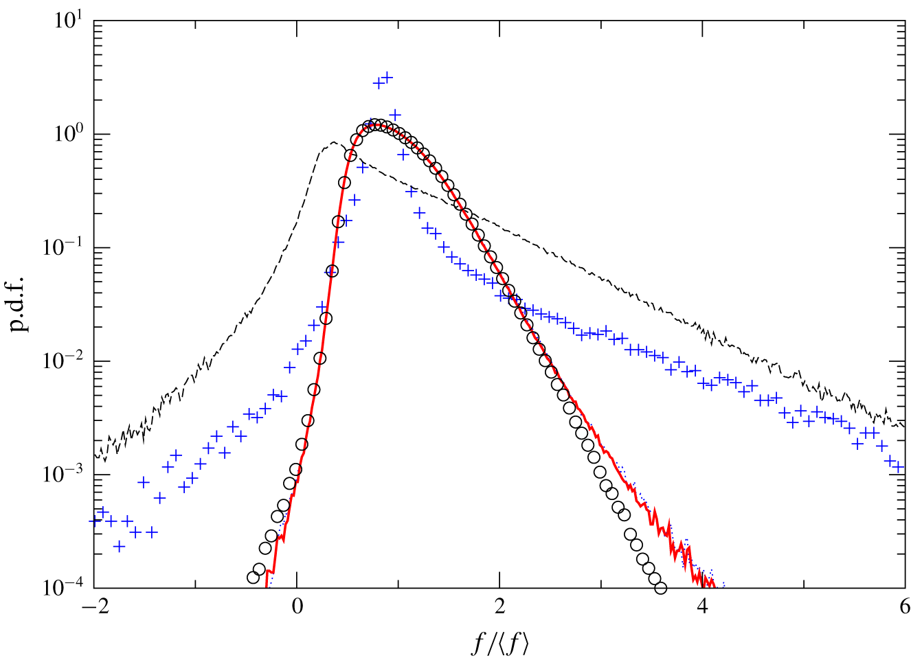
The p.d.f. of normalized friction factor  $f/\langle f\rangle$ in the pipe flow at
 $Re_{D}=8000$ with no-slip boundary condition (case 2). Plus signs,
 $36<z/R<37$ where laminar flow breakdown occurs; dashed line,
 $42<z/R<44$ where the probability of negative
 $f$ reaches its maximum; dotted line,
 $90<z/R<110$; solid line, fully developed turbulent region
 $190<z/R<210$; open circles, periodic fully developed turbulent pipe flow at
 $Re_{D}=8000$ (case 4).

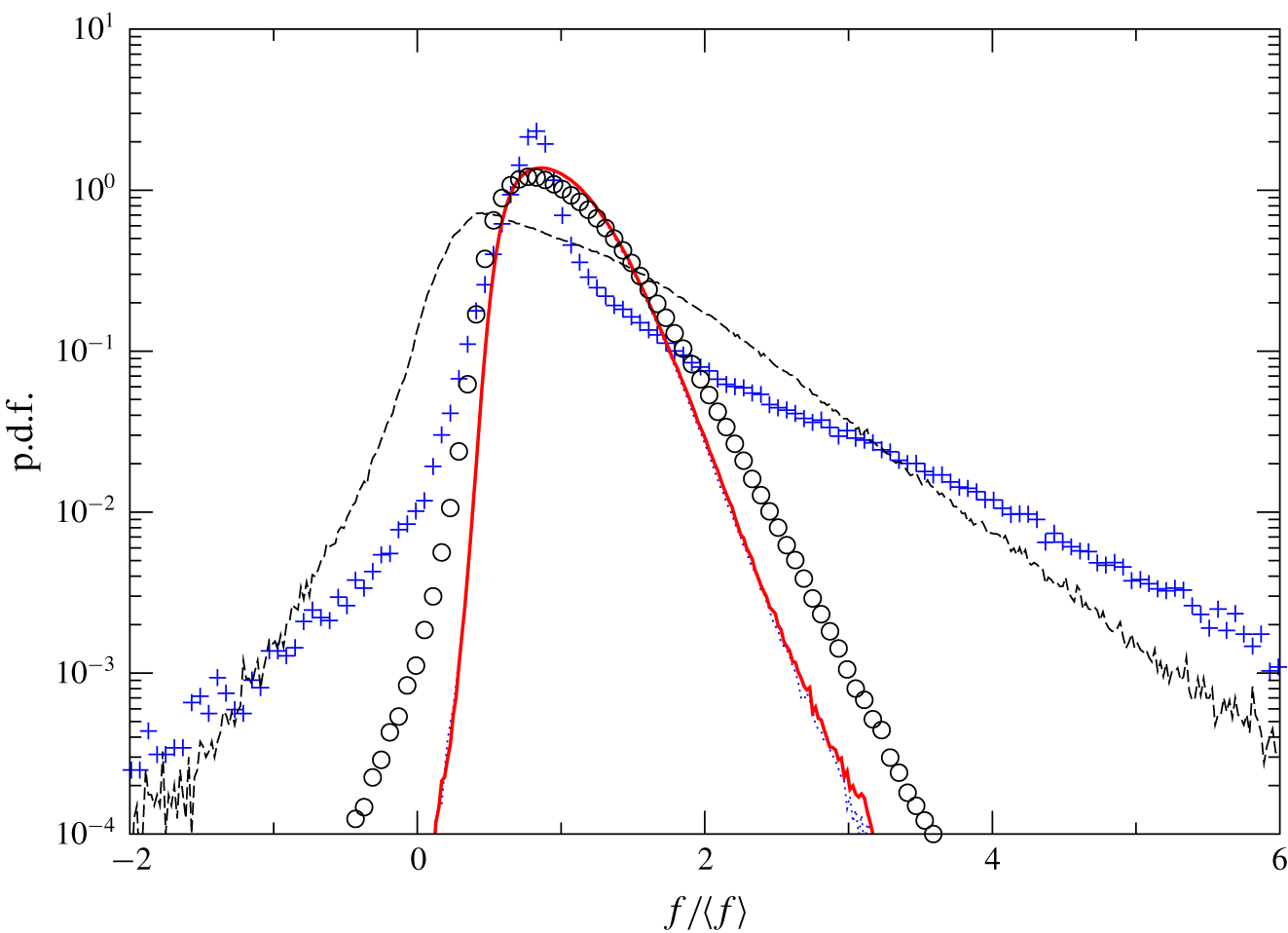
The p.d.f. of normalized friction factor  $f/\langle f\rangle$ in the pipe flow with slip boundary condition (case 3) at
 $Re_{D}=8000$. Plus signs,
 $36<z/R<37$ where laminar flow breakdown occurs; dashed line,
 $42<z/R<44$ where the probability of negative
 $f$ reaches its maximum; dotted line,
 $90<z/R<110$; solid line, fully developed turbulent region
 $190<z/R<210$; open circles, periodic fully developed turbulent pipe flow with no-slip boundary condition at
 $Re_{D}=8000$ (case 4).

The p.d.f. profiles of normalized instantaneous skin friction over four selected regions in the no-slip pipe flow case 2 are presented in figure 7. The two transitional profiles exhibit characteristics analogous to those in figure 5 for the transitional ZPGSFPBL. In particular, the profile covering the breakdown region  $36<z/R<37$ is relatively more narrowband with a high sharp peak located at
 $f/\langle f\rangle \approx 0.9$ reinforced by a noticeable bending in the region
 $1<f/\langle f\rangle <1.5$. The transitional p.d.f. profile sampled over
 $42<z/R<44$ where the maximum probability of negative skin friction is attained is also similar to its counterpart in the boundary layer. The peak is found further to the left at
 $f/\langle f\rangle \approx 0.4$, and the profile has non-negligible p.d.f. values (
 ${>}10^{-4}$ for pipe flow) over the wide range of
 $-2<f/\langle f\rangle <6$. Two turbulent p.d.f. profiles are also shown in figure 7:
 $90<z/R<110$ shortly after the completion of transition, and
 $190<z/R<210$ where the flow has reached the fully developed turbulent state. For comparison purposes, the p.d.f. profile extracted from the auxiliary case 4 is also included. It is seen that the three sets of turbulent flow results collapse over the range
 $0<f/\langle f\rangle <2$, demonstrating excellent consistency. At the threshold station
 $f/\langle f\rangle =0$, the turbulent p.d.f. profiles attain the value
 $0.001$, two orders of magnitude less than the corresponding value in the transitional p.d.f. sampled over the region of
 $42<z/R<44$. P.d.f. profiles for the slip boundary condition case 3 over the same four selected zones are given in figure 8. The two transitional profiles are analogous to those in case 2, consistent with the notion that, for the given inlet condition and the slip length, the current pipe transition process is not noticeably affected by the slip surface condition. The two turbulent profiles of figure 8 are more narrowband compared to their counterparts in figure 7 for the no-slip pipe flow. They show that, inside these two turbulent regions of the slip pipe flow, negative skin friction does not have a p.d.f. value larger than
 $10^{-4}$.
4 Number density and size of negative skin-friction patches
In figures 4 and 6 the probabilities are defined using the ratio of the surface area with negative skin friction to the total surface area, and both figures exhibit larger probability values during transition than in the downstream fully turbulent region. One follow-up question that arises naturally is whether the larger probability attained during transition is due to more frequent occurrence of isolated negative skin-friction patches or substantially larger size of such patches, or both. To address this question, we wrote a linked-list-based computer program to automatically identify, count and measure the size of each isolated patch with negative skin friction. The procedures are as follows. Step (i) is to extract the isosurfaces of streamwise velocity at a very small negative value ( $-10^{-3}U_{f}$ for the ZPGSFPBL and
 $-10^{-3}V$ for the pipe) from a selected raw DNS volume file and write them into a finite element three-dimensional surface data file. In this extraction process, the coordinates of the isosurfaces are exported into the finite element surface data file. Step (ii) is to check the connectivity of each element with all the other elements in the finite element file so that elements belonging to the same isolated patch are stored into one linked list. This step is quite inefficient but works well here because the number of isolated negative skin-friction patches is quite limited, and there is no tangling of neighbouring patches. Step (iii) is to count the number of isolated patches, and to find the area and geometric centre of each patch, from the finite element file corresponding to the originally selected raw DNS data volume. Steps (i) and (iii) are repeated for all the raw DNS files to be sampled to accumulate statistics.
(a) Number density of negative skin-friction events as a function of  $Re_{\unicode[STIX]{x1D703}}$, computed as the number
 $N$ of isolated
 $C_{f}<0$ patches per unit area
 $\unicode[STIX]{x1D703}_{0}^{2}$ and per unit time
 $\unicode[STIX]{x1D703}_{0}/U_{f}$. (b) Averaged area of isolated
 $C_{f}<0$ patches as a function of
 $Re_{\unicode[STIX]{x1D703}}$. Data from the transitional and turbulent ZPGSFPBL (case 1). At
 $Re_{\unicode[STIX]{x1D703}}=380$,
 $\unicode[STIX]{x1D6FF}=47\unicode[STIX]{x1D703}_{0}$; at
 $Re=1000$,
 $\unicode[STIX]{x1D6FF}=117\unicode[STIX]{x1D703}_{0}$,
 $Re_{\unicode[STIX]{x1D70F}}=\unicode[STIX]{x1D6FF}u_{\unicode[STIX]{x1D70F}}/\unicode[STIX]{x1D708}=439$; and at
 $Re_{\unicode[STIX]{x1D703}}=2600$,
 $\unicode[STIX]{x1D6FF}=271\unicode[STIX]{x1D703}_{0}$,
 $Re_{\unicode[STIX]{x1D70F}}=890$.

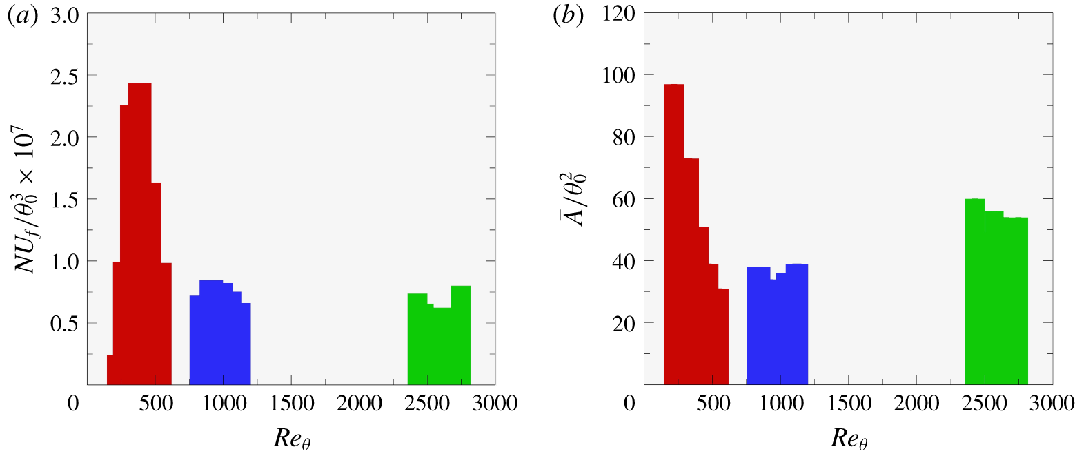
Figure 9(a) shows the number density of isolated  $C_{f}<0$ patches inside three selected streamwise zones of the ZPGSFPBL: the transitional zone of
 $80<Re_{\unicode[STIX]{x1D703}}<570$, the low-Reynolds-number turbulent zone of
 $800<Re_{\unicode[STIX]{x1D703}}<1200$, and the (relatively) high-Reynolds-number turbulent zone of
 $2400<Re_{\unicode[STIX]{x1D703}}<2800$. Within each zone, the statistics are binned to increase sample size at a uniform bin size of
 $400\unicode[STIX]{x1D703}_{0}$ along the streamwise direction. The number density is computed using the number of identified isolated
 $C_{f}<0$ patches within each bin normalized by the surface area covered by the bin and the time duration of the sampling. It is evident that, at the streamwise station where the peak of the probability of
 $C_{f}<0$ is located,
 $370<Re_{\unicode[STIX]{x1D703}}<390$ (figure 4), the number density of isolated
 $C_{f}<0$ patches also reaches its peak (figure 9a). The number densities in the two turbulent flow zones are nearly the same, and are less than
 $40\,\%$ of the peak in the transitional zone. Figure 9(b) shows the area of isolated
 $C_{f}<0$ patches (three-dimensional isosurfaces of
 $-10^{-3}U_{f}$) sampled from the same regions as in figure 9(a). It is seen that over
 $370<Re_{\unicode[STIX]{x1D703}}<390$ the averaged area is not noticeably larger than those in the two turbulent zones. Thus, the large peak in the probability of
 $C_{f}<0$ found in figure 4 for the ZPGSFPBL is primarily due to the increased number density of isolated
 $C_{f}<0$ patches during transition. Unit conversion information is given in the caption of figure 9 so that the inlet momentum thickness
 $\unicode[STIX]{x1D703}_{0}$ can be easily converted to local boundary layer thickness or viscous length scale. Additionally, the combined information contained in figure 9(a,b) suggests that the slight increase in the probability of
 $C_{f}<0$ with
 $Re_{\unicode[STIX]{x1D703}}$ for turbulent ZPGSFPBL after transition (figure 4; see also Lenaers et al. Reference Lenaers, Li, Brethouwer, Schlatter and Örlü2012) is mostly due to the increased area of isolated
 $C_{f}<0$ patches.
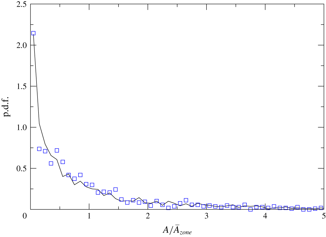
Yet another question related to the size of the isolated  $C_{f}<0$ patches is whether most of the patches have area values of
 $A$ close to their mean. Figure 10 plots the p.d.f. of normalized area
 $A/\overline{A}_{zone}$ for the ZPGSFPBL. Two zones are considered: a transitional zone
 $80<Re_{\unicode[STIX]{x1D703}}<570$, and a fully turbulent zone
 $2400<Re_{\unicode[STIX]{x1D703}}<2800$. Here
 $\overline{A}_{zone}$ is the averaged area of the negative skin-friction patches found in each zone. The two p.d.f. profiles are similar, and they are not centred around the respective mean
 $A/\overline{A}_{zone}=1$. It is seen that there is a higher probability for the occurrence of patches with area
 $A$ far less than
 $\overline{A}_{zone}$. At the same time, there is also non-negligible probability for patches with area values much larger than
 $\overline{A}_{zone}$.
The p.d.f. for the normalized area  $A/\overline{A}_{zone}$ of isolated
 $C_{f}<0$ patches in the transitional and turbulent ZPGSFPBL (case 1). Solid line, within the transition zone
 $80<Re_{\unicode[STIX]{x1D703}}<570$; open squares, within the fully turbulent zone
 $2400<Re<2800$. Here
 $\overline{A}_{zone}$ is the averaged area of the isolated
 $C_{f}<0$ patches in each respective zone.

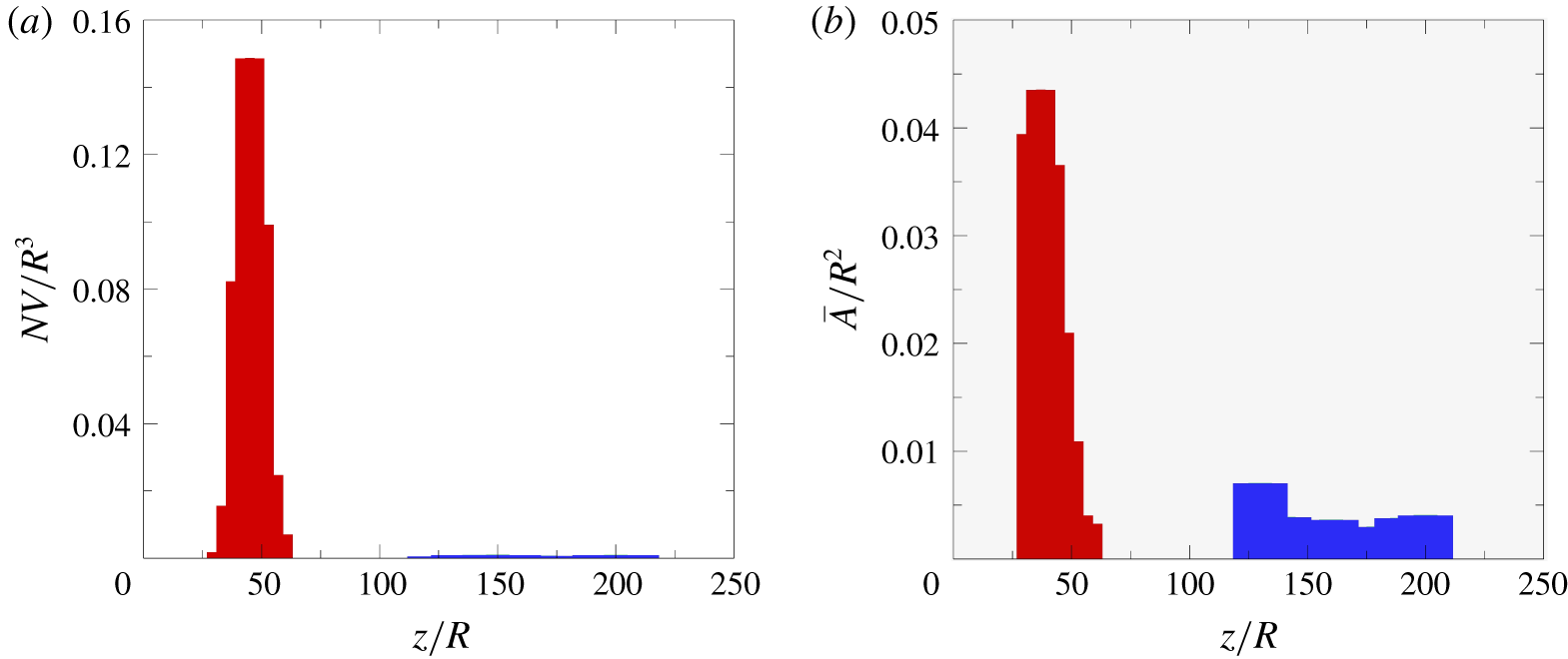
The number density and area of isolated  $f<0$ patches in case 2 are given in figures 11(a) and 11(b), respectively. The drastic difference between the number densities in the transitional zone (red) and in the fully developed turbulent zone (blue) as depicted in figure 11(a) confirms that the elevated probability of isolated
 $f<0$ patches (on average
 $1.4\,\%$ versus
 $0.017\,\%$) is primarily due to the more frequent occurrence of the patches during transition. As shown in figure 11(b), the averaged area of the patches is also several factors larger during transition than in the fully developed turbulent region. Thus increased patch area also plays a secondary role in facilitating the elevated probability of
 $f<0$ in the late stage of pipe transition. In comparison, data contained in figure 9(b) for the ZPGSFPBL do not show as large difference in the averaged patch areas during and after transition. In case 2,
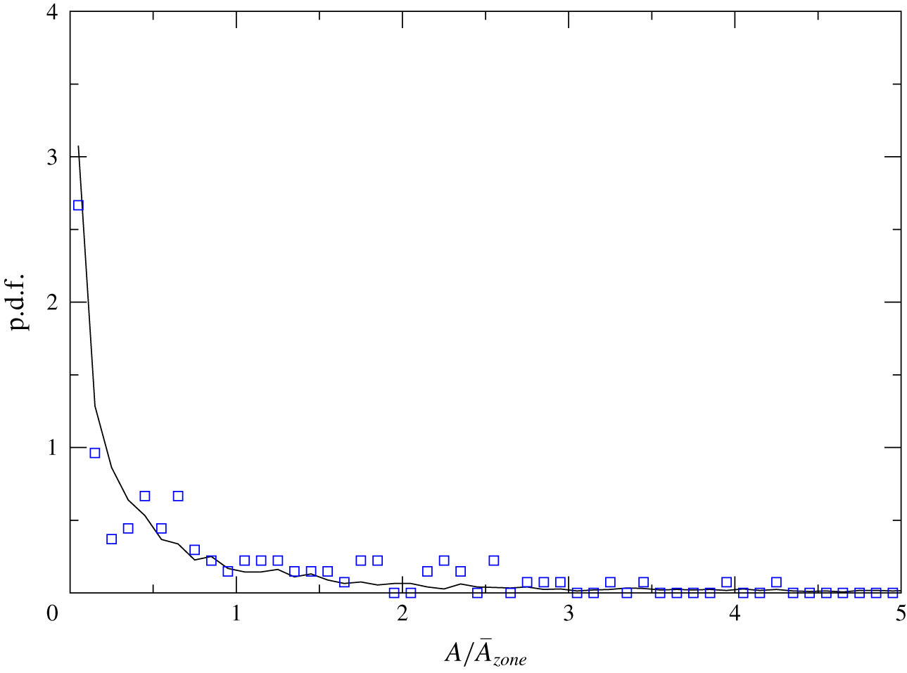
 $Re_{\unicode[STIX]{x1D70F}}=u_{\unicode[STIX]{x1D70F}}R/\unicode[STIX]{x1D708}=258.5$, which can be used to easily convert the length scale in figure 11 to viscous units. P.d.f. profiles of
 $A/\overline{A}_{zone}$ inside the same two transitional and turbulent zones for case 2 are presented in figure 12. The two profiles in figure 12 are similar to each other, and they are also analogous to the boundary layer results of figure 10: the p.d.f.s decrease monotonically with increasing
 $A/\overline{A}_{zone}$, and the probability of very large isolated
 $f<0$ patches
 $(A\sim 5\overline{A}_{zone})$ is small but non-negligible.
(a) Number density of negative skin-friction events as a function of  $z/R$, computed as the number
 $N$ of isolated
 $f<0$ patches per unit area
 $R^{2}$ and per unit time
 $R/V$. (b) Averaged area of isolated
 $f<0$ patches. Data sampled from case 2 (no-slip),
 $Re_{\unicode[STIX]{x1D70F}}=u_{\unicode[STIX]{x1D70F}}R/\unicode[STIX]{x1D708}=258.5$.

The p.d.f. for the normalized area  $A/\overline{A}_{zone}$ of isolated
 $f<0$ patches in the spatially developing no-slip pipe flow (case 2). Solid line, within the transitional zone
 $30.5<Re_{\unicode[STIX]{x1D703}}<61$; open squares, within the fully turbulent zone
 $122<Re_{\unicode[STIX]{x1D703}}<213.5$. Here
 $\overline{A}_{zone}$ is the averaged area of the isolated
 $f<0$ patches in each respective zone.

Turbulent flows under an intermediate strength level of adverse pressure gradient may experience incipient detachment in which the probability of instantaneous backflow is less than  $1\,\%$. A large amount of work has been done on such flows using the flat-plate and airfoil-type configurations, and research in that area was summarized in the review of Simpson (Reference Simpson1989). Recent DNS work on this subject was reported by Vinuesa, Örlü & Schlatter (Reference Vinuesa, Örlü and Schlatter2017) in which the instantaneous backflow events were studied for turbulent flow over the suction side of a wing section, experiencing an increasing adverse pressure gradient without mean flow separation. They showed that, at moderate adverse pressure gradient level, the backflow events are connected to the near-wall turbulence structures, whereas at stronger adverse pressure gradient level, the backflow events are more closely connected to the outer part of the flow. More interestingly, their results also suggest that increasing probability of
 $C_{f}<0$ is primarily due to the increased number density of isolated
 $C_{f}<0$ patches rather than the local size. We found that the increased probability is primarily due to an enhanced number density of the backflow events coupled with a notable increase in the wall footprint size of such events. But it must be pointed out that, in our view,
 $C_{f}<0$ events in the ZPGSFPBL and in pipe flows are fundamentally from the backflow events under adverse pressure gradient flows because the latter ones are totally expected as their carrier flows are on the path towards mean-flow separation.
5 Wall-normal extent of incipient backflow
Given the statistical importance of the negative instantaneous skin friction during transition, it is quite logical then to inquire about the wall-normal extent of the incipient backflow. Previous work by Lenaers et al. (Reference Lenaers, Li, Brethouwer, Schlatter and Örlü2012) and Willert et al. (Reference Willert, Cuvier, Foucaut, Klinner, Stanislas, Laval, Srinath, Soria, Amili and Atkinson2018) suggested that in the fully turbulent ZPGSFPBL the instantaneous backflow region is contained within the first  $8$ and
 $5$ wall units from the plate, respectively. Jalalabadi & Sung (Reference Jalalabadi and Sung2018) found that in fully developed turbulent pipe flow the wall-normal extent of the backflow is within the first
 $4$ wall units. Is the statistically more significant instantaneous backflow during transition also similarly confined along the wall-normal direction?
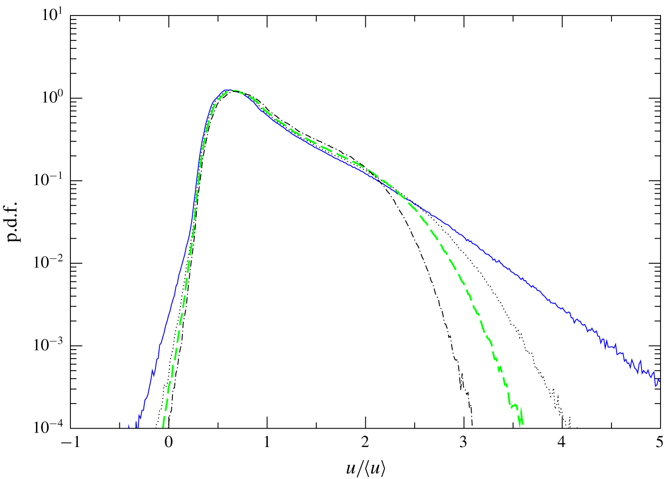
Figure 13 presents, for the boundary layer case 1, the p.d.f. of the normalized instantaneous streamwise velocity  $u/\langle u\rangle$ over a set of four wall-parallel planes in the transitional region where the probability of negative skin friction reaches its peak,
 $370<Re_{\unicode[STIX]{x1D703}}<390$. Figure 13 shows that the plane closest to the wall (
 $y/\unicode[STIX]{x1D6FF}=0.018$) has the strongest broadband characteristic: its p.d.f. values at
 $u/\langle u\rangle =5$ and
 $-0.35$ are
 $3.5\times 10^{-4}$ and
 $1.0\times 10^{-4}$, respectively, the largest among all four planes. This implies that streamwise flow in the immediate vicinity of the wall during transition has the biggest variation range with respect to its mean. Figure 13 also shows clearly that the instantaneous backflow over
 $370<Re_{\unicode[STIX]{x1D703}}<390$ covers up to
 $5\,\%$ of the boundary layer thickness, based on the p.d.f. threshold value of
 $1.0\times 10^{-4}$. P.d.f. profiles of
 $u/\langle u\rangle$ over a set of four wall-parallel planes
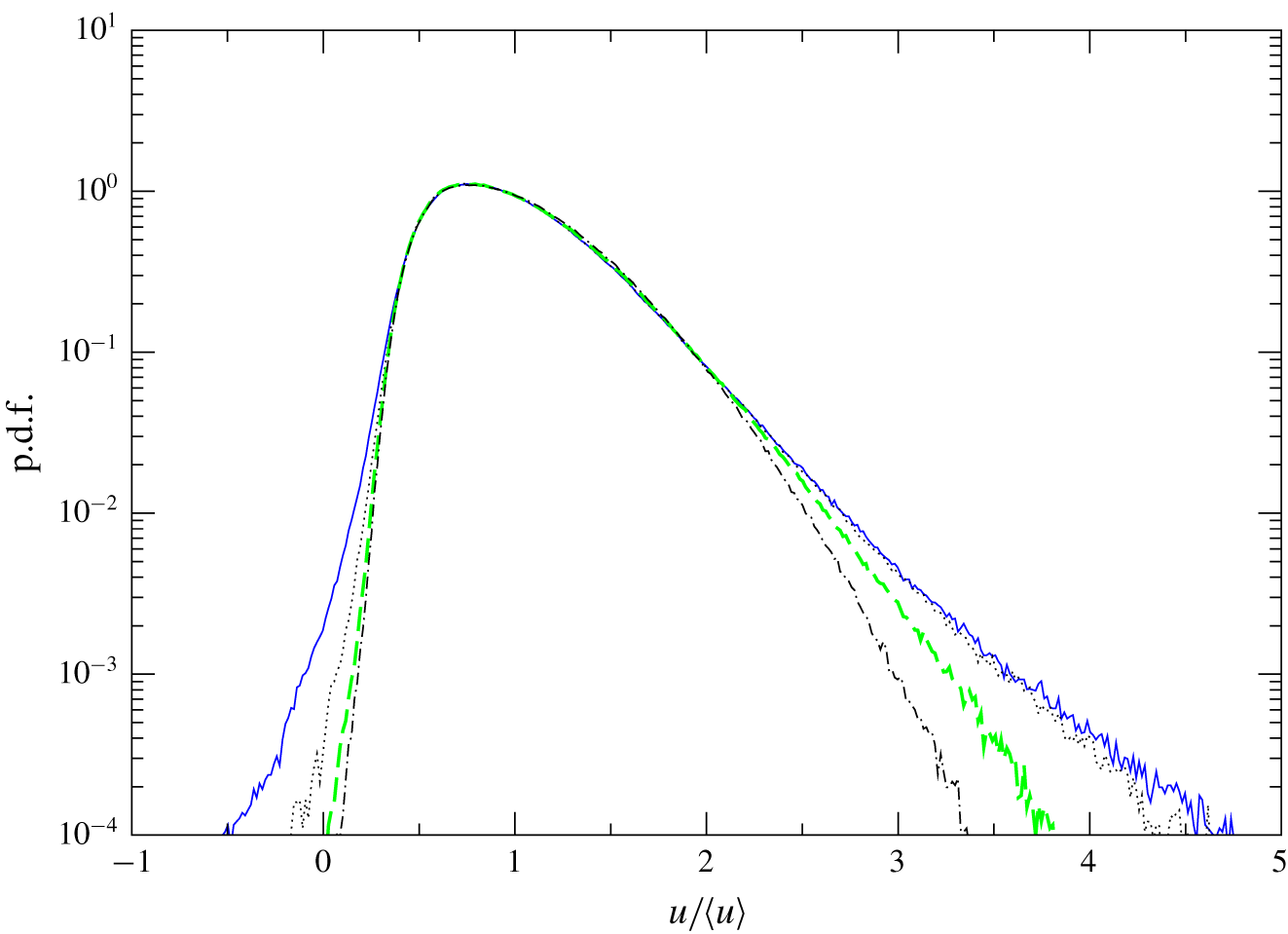
 $(0.24<y^{+}<4.8)$ in the fully turbulent ZPGSFPBL are given in figure 14 over the region
 $2790<Re_{\unicode[STIX]{x1D703}}<2810$. The plane closest to the wall covers the largest variation range of
 $u/\langle u\rangle$, analogous to the observation made in figure 13 for the transitional boundary layer. For p.d.f. values higher than
 $0.1$, the four profiles nearly collapse. This seems to suggest that, inside the viscous sublayer, the more frequent events surrounding the mean have nearly the same likelihood. Figure 14 also shows clearly that, based on the p.d.f. threshold value of
 $1.0\times 10^{-4}$, the negative instantaneous backflow is confined within the first
 $4$ wall units in the fully turbulent ZPGSFPBL, consistent with Lenaers et al. (Reference Lenaers, Li, Brethouwer, Schlatter and Örlü2012) and Willert et al. (Reference Willert, Cuvier, Foucaut, Klinner, Stanislas, Laval, Srinath, Soria, Amili and Atkinson2018).
The p.d.f. of normalized streamwise velocity  $u/\langle u\rangle$ over a set of wall-parallel planes in the transitional ZPGSFPBL at
 $370<Re_{\unicode[STIX]{x1D703}}<390$ where the probability of negative
 $C_{f}$ reaches its maximum. Solid line,
 $y/\unicode[STIX]{x1D6FF}=0.018$; dotted line,
 $y/\unicode[STIX]{x1D6FF}=0.032$; dashed line,
 $y/\unicode[STIX]{x1D6FF}=0.039$; dot-dashed line:
 $y/\unicode[STIX]{x1D6FF}=0.050$.

The p.d.f. of normalized streamwise velocity  $u/\langle u\rangle$ over a set of wall-parallel planes in the turbulent ZPGSFPBL at
 $2790<Re_{\unicode[STIX]{x1D703}}<2810$. Solid line,
 $y^{+}=0.24$; dotted line,
 $y^{+}=2.2$; dashed line,
 $y^{+}=3.8$; dot-dashed line,
 $y^{+}=4.8$.

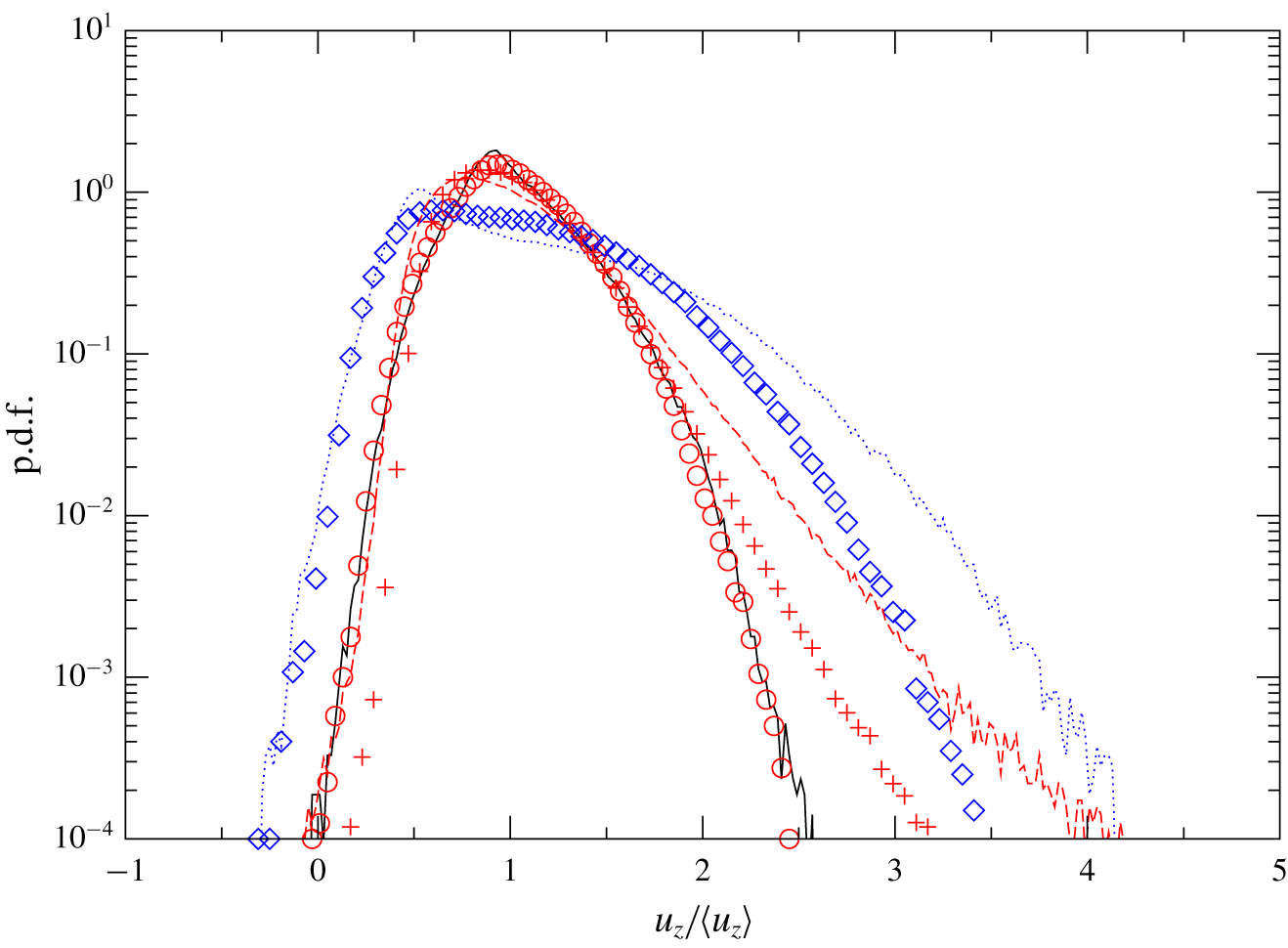
Figure 15 plots, for case 2 and case 3, the p.d.f.s of the normalized instantaneous axial velocity  $u_{z}/\langle u_{z}\rangle$ over two coaxial cylindrical planes in the transitional region
 $(42<z/R<44)$, as well as over one coaxial plane in the fully developed turbulent region
 $190<z/R<210$. Similar to the transitional boundary layer results in figure 13, the p.d.f. for the plane close to the wall
 $(1-r=0.049R)$ covers the widest spectrum of velocity variation range. The instantaneous backflow in both the no-slip and slip cases extends from the wall to
 $0.18R$, based on the p.d.f. threshold value of
 $1.0\times 10^{-4}$. This shows that during pipe transition a sizeable portion of the radial range could potentially be occupied by instantaneous backflow. In contrast, figure 15 also shows that, for the no-slip case 2, over the region where the pipe flow is in a fully developed turbulent state, the instantaneous backflow only extends to
 $0.0055R$. Figure 15 also confirms that, with the slip boundary condition in case 3, there is almost no indication of instantaneous backflow in the fully developed turbulent region.
The p.d.f. of normalized axial velocity  $u_{z}/\langle u_{z}\rangle$ in the spatially developing pipe flows at
 $Re_{D}=8000$. Lines, no-slip (case 2); symbols, slip (case 3). Over the transitional region
 $42<z/R<44$ where the probability of negative
 $f$ reaches its maximum: dotted line and diamonds,
 $(1-r)/R=0.049$; solid line and circles, 0.18. Over the fully developed turbulent region
 $190<z/R<210$: dashed line and plus signs,
 $(1-r)/R=0.0055$.

6 Wall shear stress vector near negative skin-friction patches
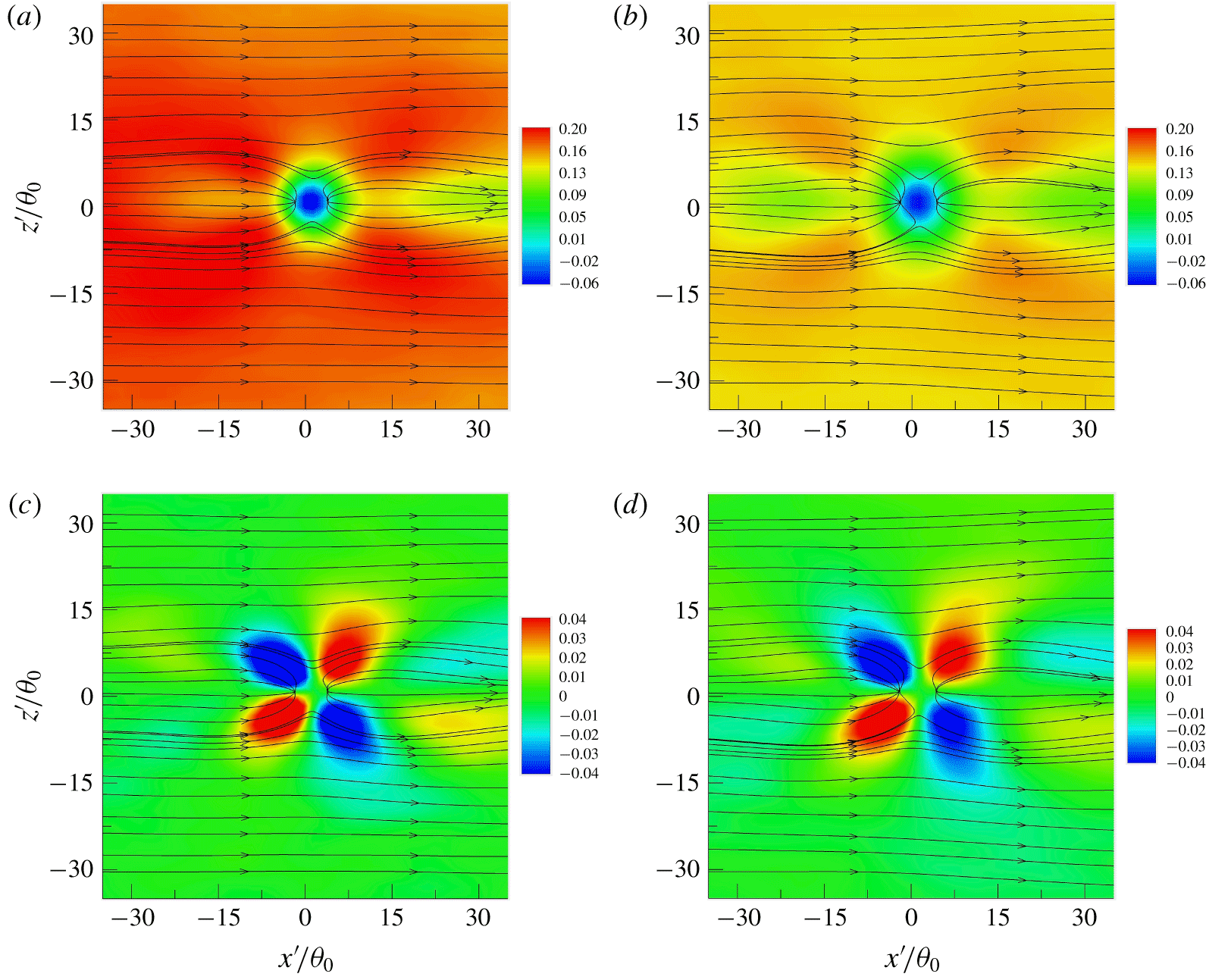
Because the geometric centre of each negative skin-friction patch has been determined through the automatic identification and counting process, it is straightforward to perform conditional averaging of the wall stress vector in the vicinity of these identified patches. A pair of square brackets indicates such conditional averaging. Figures 16(a) and 16(b) show, for the ZPGSFPBL in case 1, the conditionally averaged wall shear stress lines overlaid on the contours of  $[\unicode[STIX]{x2202}u/\unicode[STIX]{x2202}y]_{wall}$ in the transitional region of
 $80<Re_{\unicode[STIX]{x1D703}}<570$ and the fully turbulent region of
 $2400<Re_{\unicode[STIX]{x1D703}}<2800$, respectively. Here
 $x^{\prime }$ and
 $z^{\prime }$ are the streamwise and spanwise offsets from the identified patch centre, respectively. The turbulent-region contours of figure 16(b) confirm that the averaged shape of the negative skin-friction patches is circular, as found earlier by Lenaers et al. (Reference Lenaers, Li, Brethouwer, Schlatter and Örlü2012). The diameter of the circle at
 $2400<Re_{\unicode[STIX]{x1D703}}<2800$ is approximately
 $6.5\unicode[STIX]{x1D703}_{0}$, equivalent to
 $21$ wall units, also in excellent agreement with Lenaers et al. (Reference Lenaers, Li, Brethouwer, Schlatter and Örlü2012). Note that the two-dimensional area of
 $[\unicode[STIX]{x2202}u/\unicode[STIX]{x2202}y]_{wall}<0$ inferred by this diameter is less than the three-dimensional isosurface area of
 $-10^{-3}U_{f}$ shown in figure 9(b). Cardesa et al. (Reference Cardesa, Monty, Soria and Chong2014) mentioned negative flow present in a long wake behind the patch lasting for several hundred wall units: that feature is not found in the current study, and it was not reported in either the channel/ZPGSFPBL of Lenaers et al. (Reference Lenaers, Li, Brethouwer, Schlatter and Örlü2012) or the pipe flow of Jalalabadi & Sung (Reference Jalalabadi and Sung2018). A sink critical point and a source critical point exist in the fore and aft of the average circle, respectively. The results of Chin et al. (Reference Chin, Monty, Chong and Marusic2018) show similar features – one distinction is that their results are averaged based on the condition that there must be two critical points in a patch, whereas the present results are only conditioned on the geometric centre of a negative skin-friction patch. Figure 16(c,d) shows the conditionally averaged wall shear stress lines overlaid on the contours of
 $[\unicode[STIX]{x2202}w/\unicode[STIX]{x2202}y]_{wall}$ in the transitional region of
 $80<Re_{\unicode[STIX]{x1D703}}<570$ and the fully turbulent region of
 $2400<Re_{\unicode[STIX]{x1D703}}<2800$, respectively. The results are in overall agreement with Cardesa et al. (Reference Cardesa, Monty, Soria and Chong2014) and Chin et al. (Reference Chin, Monty, Chong and Marusic2018), and imply strong spanwise variation of the wall shear stress field near the negative skin-friction patches. See also Brücker (Reference Brücker2015).
Direction and magnitude of wall shear stress vector conditionally averaged in the vicinity of the wall-plane centre of  $C_{f}<0$ patches in the ZPGSFPBL (case 1). (a,b) Wall shear lines overlaid on the contours of
 $\unicode[STIX]{x2202}[u]/\unicode[STIX]{x2202}y|_{wall}(\unicode[STIX]{x1D703}_{0}/U_{f})$. (c,d) Wall shear lines overlaid on the contours of
 $\unicode[STIX]{x2202}[w]/\unicode[STIX]{x2202}y|_{wall}(\unicode[STIX]{x1D703}_{0}/U_{f})$. (a,c) Over the transition region
 $80<Re_{\unicode[STIX]{x1D703}}<570$; (b,d) over the fully turbulent region
 $2400<Re_{\unicode[STIX]{x1D703}}<2800$.

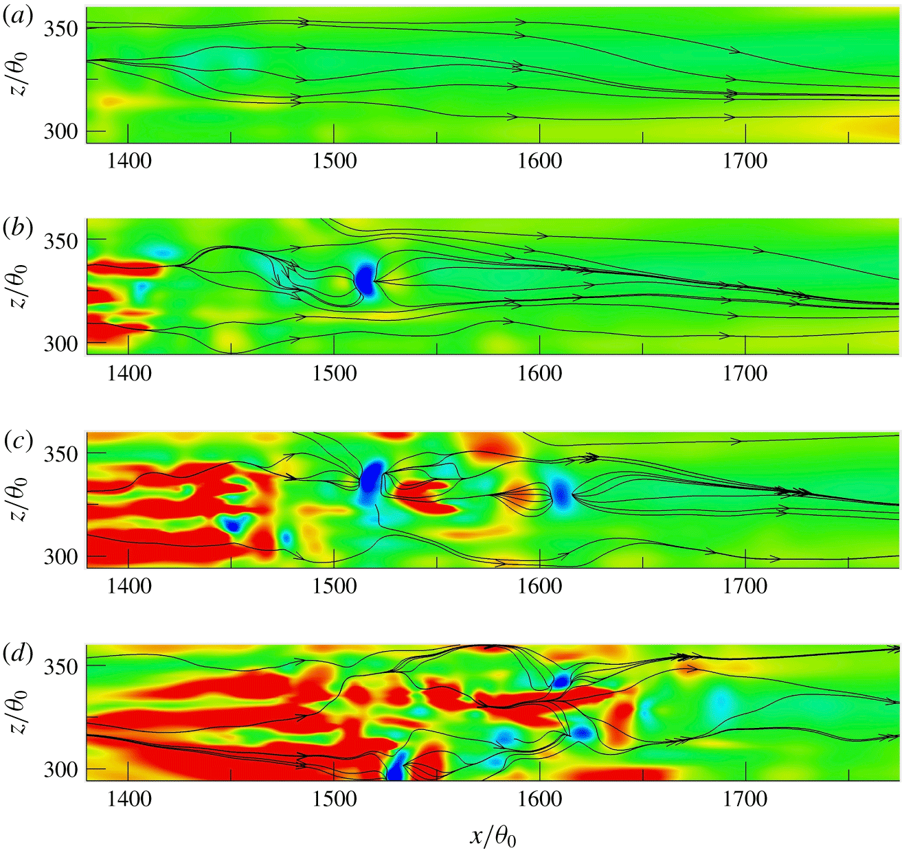
It should be noted that, although the averaged shape of the negative skin-friction patch is circular, the instantaneous patches do not have to be. This is confirmed in figure 17 where the instantaneous wall shear stress lines are plotted together with the contours of  $\unicode[STIX]{x2202}u/\unicode[STIX]{x2202}y|_{wall}$ at four consecutive instants in a transitional region of the ZPGSFPBL. The momentum-thickness Reynolds number
 $Re_{\unicode[STIX]{x1D703}}$ varies from
 $240$ to
 $300$ in this region. It is obvious from figure 17 that no instantaneous negative skin-friction patch is circular as suggested by the averaged image in figure 16. Thus, one must exercise caution when inferring flow structures from conditionally averaged images. Many of the instantaneous patches in figure 17 are associated with a sink/source critical point pair. Further, the kidney-shaped blue patch located at
 $1500<x/\unicode[STIX]{x1D703}_{0}<1550$ at
 $t=102\,000\,\unicode[STIX]{x0394}t$ hardly changes its position later at
 $t=102\,100\,\unicode[STIX]{x0394}t$. However, it is nowhere to be found at either the earlier instant
 $t=101\,900\,\unicode[STIX]{x0394}t$ nor the subsequent instant
 $t=102\,200\,\unicode[STIX]{x0394}t$. Examination of many similar image sequences suggests that the lifetime of the negative skin-friction patches is usually small, less than
 $100\unicode[STIX]{x0394}t~({\approx}112.5\unicode[STIX]{x1D703}_{0}/U_{f})$, and is insensitive to the Reynolds-number range. This time interval is equivalent to approximately
 $0.4\unicode[STIX]{x1D6FF}/U_{f}$ or
 $15\unicode[STIX]{x1D708}/u_{\unicode[STIX]{x1D70F}}^{2}$ in the fully turbulent region at
 $Re_{\unicode[STIX]{x1D703}}=2600$.
Instantaneous wall-shear stress lines and contours of  $\unicode[STIX]{x2202}u/\unicode[STIX]{x2202}y|_{wall}(\unicode[STIX]{x1D703}_{0}/U_{f})$: (a)
 $t=101\,900\unicode[STIX]{x0394}t$; (b)
 $t=102\,000\unicode[STIX]{x0394}t$; (c)
 $t=102\,100\unicode[STIX]{x0394}t$; and (d)
 $t=102\,200\unicode[STIX]{x0394}t$. The contour levels are the same as those in figure 16(a). The time and spatial locations here are related to those in figure 18: the blue patch of
 $C_{f}<0$ in panel (b) at
 $t=102\,000\unicode[STIX]{x0394}t$ is the same as that revealed in the three-dimensional image of figure 18(b).

7 Vortex structure associated with negative skin-friction patches
The next question to address is what kind of vortex structure is responsible for the generation of negative skin-friction patches during the transition processes of the ZPGSFPBL and the pipe flow. Previous work in a fully turbulent boundary layer by Lenaers et al. (Reference Lenaers, Li, Brethouwer, Schlatter and Örlü2012) suggests that the rare backflow is related to the presence of an oblique vortex associated with a low-speed streak. For fully developed turbulent pipe flow, Jalalabadi & Sung (Reference Jalalabadi and Sung2018) showed that a buffer layer spanwise vortex is at play; Chin et al. (Reference Chin, Monty, Chong and Marusic2018) suggested that the conditionally averaged vortex field surrounding a pair of critical points contains two hairpin vortices: a downstream reverse hairpin vortex, whose head element is directed towards the wall, and an upstream normal hairpin vortex. Our transitional flow and turbulent flow results improve upon those previous findings acquired from fully turbulent flows.
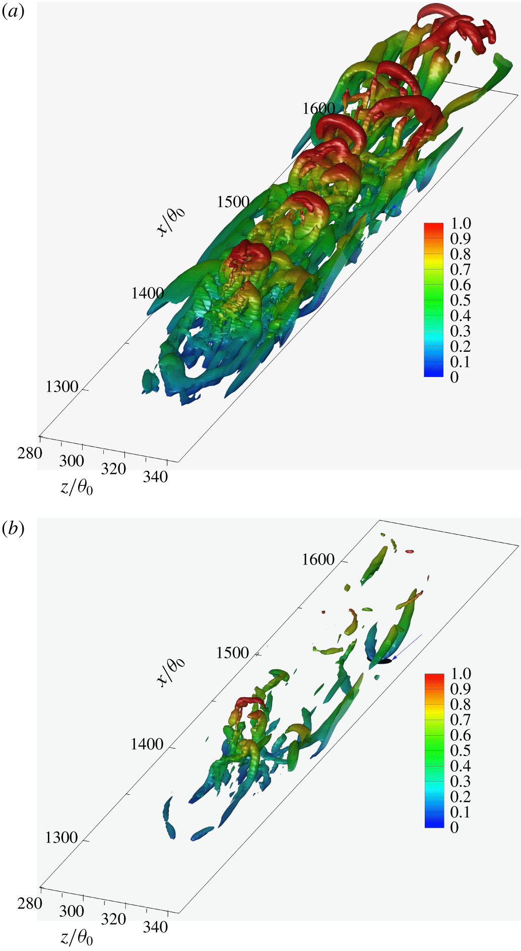
Figure 18(a) shows a young transitional–turbulent spot in the ZPGSFPBL of case 1 at the instant  $t=102\,000\,\unicode[STIX]{x0394}t$ using the isosurfaces of swirling strength
 $\unicode[STIX]{x1D706}_{ci}$ (Adrian Reference Adrian2007) coloured by the relative wall-normal coordinate
 $y/\unicode[STIX]{x1D6FF}$. The time and location are the same as those of figure 17(b). It is seen that the young spot consists mainly of concentrated normal hairpin vortices that are inclined downstream with their head elements directed away from the wall, some even extruding outside the boundary layer. This has been well known through DNS studies over the past decade on boundary layer transition (Wu & Moin Reference Wu and Moin2009; Park et al. Reference Park, Wallace and Wu2012; Zheng, Yang & Chen Reference Zheng, Yang and Chen2016). In figure 18(a), the isosurface of
 $u/U_{f}=-0.01$, coloured in black and highlighted with an arrow, is also included. However, the view to this negative patch is blocked by the dominance of the normal hairpin vortices. To make the incipient backflow region visible, the isosurface value of the swirling strength is increased by a factor of more than
 $3$ in figure 18(b). As a result, most of the vortex structures are removed from view due to their weaker swirling strength. This reveals clearly the incipient backflow region located underneath the head element of a reverse hairpin vortex structure. This three-dimensional incipient backflow structure is the same as the kidney-shaped two-dimensional patch shown in figure 17(b). The reverse hairpin vortex has strong swirling strength since it has survived the sharp increase in threshold value with almost no fragmentation. It is inclined towards the downstream direction with its head element directed towards, and almost touching (blue colour), the wall. The circulation associated with the reverse hairpin’s head element in the immediate vicinity of the wall is thus responsible for the instantaneous backflow as represented by the black isosurface of
 $u/U_{f}=-0.01$. No upstream normal hairpin vortex pairing with the reverse hairpin is visible in figure 18(b).
The isosurfaces of the swirling strength  $\unicode[STIX]{x1D706}_{ci}$ associated with a boundary layer transitional–turbulent spot overlaid with the isosurface of
 $u/U_{f}=-0.01$ (black colour and highlighted with arrow) at the instant
 $t=102\,000\,\unicode[STIX]{x0394}t$ in case 1: (a)
 $\unicode[STIX]{x1D706}_{ci}=22\times 5.33\times 10^{-4}U_{f}/\unicode[STIX]{x1D703}_{0}$; (b)
 $\unicode[STIX]{x1D706}_{ci}$ increased to
 $70\times 5.33\times 10^{-4}U_{f}/\unicode[STIX]{x1D703}_{0}$ so that near-wall structures blocked in panel (a) become visible. Isosurfaces of
 $\unicode[STIX]{x1D706}_{ci}$ are coloured by the normalized wall distance
 $y/\unicode[STIX]{x1D6FF}$. The local boundary layer thickness
 $\unicode[STIX]{x1D6FF}$ is approximately
 $28\unicode[STIX]{x1D703}_{0}$.

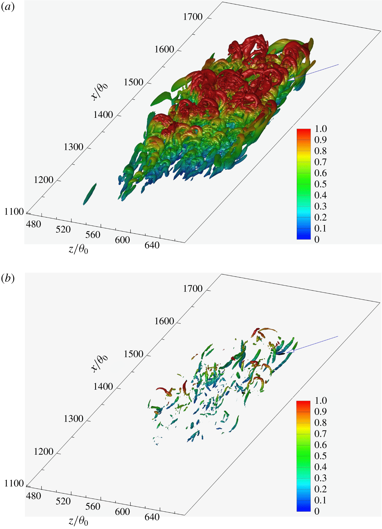
The isosurfaces of the swirling strength  $\unicode[STIX]{x1D706}_{ci}$ associated with a boundary layer transitional–turbulent spot overlaid with the isosurface of
 $u/U_{f}=-0.01$ (black colour and highlighted with arrow) at the instant
 $t=104\,900\,\unicode[STIX]{x0394}t$ in case 1: (a)
 $\unicode[STIX]{x1D706}_{ci}=22\times 5.33\times 10^{-4}U_{f}/\unicode[STIX]{x1D703}_{0}$; (b)
 $\unicode[STIX]{x1D706}_{ci}$ increased to
 $120\times 5.33\times 10^{-4}U_{f}/\unicode[STIX]{x1D703}_{0}$ so that near-wall structures blocked in panel (a) become visible. Isosurfaces of
 $\unicode[STIX]{x1D706}_{ci}$ are coloured by the normalized wall distance
 $y/\unicode[STIX]{x1D6FF}$. The local boundary layer thickness
 $\unicode[STIX]{x1D6FF}$ is approximately
 $28\unicode[STIX]{x1D703}_{0}$.

To reinforce the prevalent nature of this feature, a matured transitional–turbulent spot, at a much later instant  $t=104\,900\,\unicode[STIX]{x0394}t$ and from a different region, is shown in figure 19(a). Its structural composition is clearly a concentration of (normal) hairpin vortices with larger hairpins in the downstream portion of the spot extruding into the free stream and smaller hairpins in the upstream portion inside the boundary layer. With a factor of 6 increase of the swirling strength value from
 $\unicode[STIX]{x1D706}_{ci}=22\times 5.33\times 10^{-4}U_{f}/\unicode[STIX]{x1D703}_{0}$ to
 $120\times 5.33\times 10^{-4}U_{f}/\unicode[STIX]{x1D703}_{0}$, the original hairpin forest disintegrated with only scattered fragments left in figure 19(b). Remarkably, one reverse hairpin vortex survives the elevation in the isosurface value, and it is clearly visible in the downstream end of the spot. This suggests that it possesses stronger swirling strength than most of the normal hairpin vortices in the spot. Again, almost exactly the same as in figure 18(b), an incipient flow reversal region
 $(u/U_{f}=-0.01)$ is seen in figure 19(b) right underneath the head element of the reverse hairpin vortex. This demonstrates that, together with many other visualization images not presented in the paper, that strong reverse hairpin vortex is often the structure responsible for the instantaneous negative skin friction in our transitional ZPGSFPBL.
It is quite fascinating to realize that embedded in the ZPGSFPBL transitional–turbulent spot’s hairpin forest is some rare and very strong reverse hairpin vortex, and its head element induces near-wall instantaneous backflow.
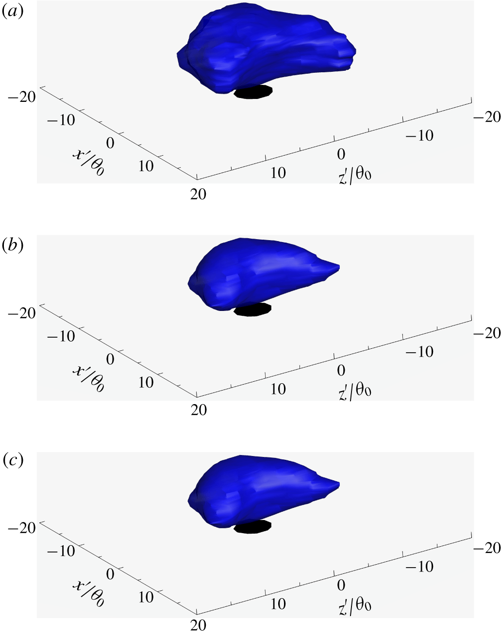
The geometric centre of each isolated  $C_{f}<0$ patch on the wall has been identified using the procedures given in § 4. The swirling strength field
 $\unicode[STIX]{x1D706}_{ci}(x,y,z,t)$ in the vicinity of each instantaneous centre in the ZPGSFPBL’s transitional region
 $80<Re_{\unicode[STIX]{x1D703}}<570$ has been (conditionally) averaged, and presented in figure 20(a) as
 $[\unicode[STIX]{x1D706}_{ci}]$. Also shown in the figure is the isosurface of conditionally averaged streamwise velocity
 $u/U_{f}=-0.001$. Similar information for the downstream low- and relatively high-Reynolds-number turbulent regions is given in figures 20(b) and 20(c), respectively. The head element and the neck element have survived the averaging. It is evident the head/neck combination curves towards the upstream direction, consistent with the instantaneous reverse hairpin structures presented in the previous two figures. In figure 20, there seems to be a stacking of layers of head/neck elements, which is likely due to the fact that the
 $\unicode[STIX]{x1D706}_{ci}(x,y,z,t)$ field is averaged in the vicinity of the wall-plane centre of an isolated
 $C_{f}<0$ patch, and the wall-normal positions of different reverse hairpins may vary. The leg elements of the instantaneous reverse hairpin vortices clear in figures 18(b) and 19(b) are not visible in the conditionally averaged field of figure 20(a). This is due to the fact that we are averaging all the
 $\unicode[STIX]{x1D706}_{ci}(x,y,z,t)$ field in the vicinity of the wall-plane centre of an isolated
 $C_{f}<0$ patch. Different reverse hairpin vortices possess different inclination angles with respect to the wall, and their sizes also vary. We even observed an instantaneous reverse hairpin vortex almost perpendicular to the wall. Generally speaking, there may be two scenarios of obtaining a conditionally averaged reverse hairpin vortex image as sharp as that in figure 18(b): (1) Most of the instantaneous reverse hairpin vortices need to be oriented in the same position with respect to the patch centre, and they should have nearly the same size and the same swirling strength: this is not possible. (2) Identify and extract each reverse hairpin vortex, rotate them to the same inclination angle and scale them to the same size and the same strength: this might be possible. Again, one should exercise extra caution when deciphering conditionally averaged coherent structures.
Isosurface of conditionally averaged swirling strength  $[\unicode[STIX]{x1D706}_{ci}]=30\times 5.33\times 10^{-4}U_{f}/\unicode[STIX]{x1D703}_{0}$ (blue) and isosurface of conditionally averaged negative streamwise velocity
 $[u]/U_{f}=-0.001$ (black) surrounding the wall-plane centre of
 $C_{f}<0$ patches in the ZPGSFPBL (case 1). Here
 $x^{\prime }$ and
 $z^{\prime }$ are the streamwise and spanwise offsets from the wall-plane centre of
 $C_{f}<0$ patches, respectively. (a) Sampled over
 $1442~C_{f}<0$ patches in the transition region
 $80<Re_{\unicode[STIX]{x1D703}}<570$; (b) sampled over
 $693~C_{f}<0$ patches in the low-Reynolds-number turbulent region
 $800<Re_{\unicode[STIX]{x1D703}}<1200$; and (c) sampled over
 $914~C_{f}<0$ patches in the fully turbulent region
 $2400<Re_{\unicode[STIX]{x1D703}}<2800$. Note that
 $[\unicode[STIX]{x1D706}_{ci}]$ is the average of all the structures over the
 $C_{f}<0$ patches. Also, because the instantaneous reverse hairpin vortices have random size and random inclination angle with respect to the wall, and they coexist with other structures, their leg elements are not easily visible after the current averaging procedure.

Figure 21 shows, for the case 3 pipe flow with slip boundary condition at one instant, the isosurfaces of swirling strength  $\unicode[STIX]{x1D706}_{ci}=3V/R$ and the isosurfaces of negative axial velocity component
 $u_{z}/V=-0.01$ (deep blue colour). The axial spatial range shown in figure 21(a) is from the inlet to
 $z/R<91$, covering the transitional region. A zoomed view focusing on the section of
 $37<z/R<46$ is given in figure 21(b). Red colour on the
 $\unicode[STIX]{x1D706}_{ci}$ isosurfaces indicates close proximity to the wall. It is evident that the instantaneous backflow region during pipe transition is often collocated with the head element of a reverse hairpin vortex whose two leg elements extend away from the wall towards the core region of the pipe flow, reinforcing the observation made in figures 18–20 for the transitional ZPGSFPBL.
Isosurfaces of  $u_{z}/V=-0.01$ (deep blue colour) overlaid on those of the swirling strength
 $\unicode[STIX]{x1D706}_{ci}=3V/R$ in the transitional and turbulent pipe flow with slip boundary condition (case 3): (a)
 $0<z/R<91$; (b)
 $37<z/R<46$. The isosurfaces of swirling strength are coloured by the radial coordinate, with red corresponding to the wall
 $r/R=1$.

8 Concluding remarks
Although it is known that extremely rare backflow events can occur in a fully turbulent ZPGSFPBL (Johansson Reference Johansson1988), the 1956 Schubauer–Klebanoff conclusion regarding the total absence of negative skin friction in ZPGSFPBL transition has remained unchallenged over the past six decades. In hindsight, such a challenge should have occurred sooner than the present work. We found pronounced (as compared to those in the fully turbulent region) negative skin-friction events during the laminar-to-turbulent transition processes of the spatially developing ZPGSFPBL. We also found qualitatively similar and quantitatively stronger negative wall shear stress events in the spatially developing transitional pipe flow with no-slip and slip boundary conditions under circumferential mode inlet disturbances. The peak probability of such events is located in the late stage of transition between the streamwise stations where the minimum and maximum mean skin friction are attained. The magnitude of the peak probability is substantially larger than the corresponding probability in the downstream fully turbulent region.
Because of the sensitivity of skin friction during transition to inflow and free-stream conditions, in order to achieve generality, it is important to ensure that the flows investigated are canonical, well researched and representative. Indeed, case 1 is such a canonical flow. In fact, it is nearly identical to the ERCOFTAC T3A case (Roach & Brierley Reference Roach and Brierley1992) with an inlet Blasius laminar boundary layer beneath  $3\,\%$ intensity of free-stream homogeneous isotropic turbulence (the integral turbulence length scale may differ). This particular flow case has been extensively used as a test case in bypass transition modelling, and it has also been used extensively in DNS studies on bypass transition mechanism. As such, the results acquired from the present study on case 1 are expected to carry generality within the category of boundary layer bypass transition in the narrow sense. The case 2 configuration corresponds to the most fundamental and the simplest internal flow, namely, smooth pipe flow with fully developed laminar inlet condition. Many landmark fundamental pipe transition studies have been performed by previous researchers on such a configuration superimposed with different types of finite-amplitude perturbations such as orifice or impulsive jets. All those studies generated results that are considered to be generally applicable to the fundamental problem of pipe transition. Here, we adopt the same philosophy. As stated, in case 2, we use a narrow numerical ring to produce the inlet disturbance. We also performed simulations by moving the numerical ring to a different location: those simulations also result in qualitatively the same type of pronounced negative skin-friction peak during transition. Of course, the quantitative peak levels vary with the imposed perturbations, but the trends remain the same.
For the present ZPGSFPBL, the maximum probability of negative skin friction,  $0.3\,\%$, is found between the onset of breakdown and the completion of transition. Over the transitional range of
 $200<Re_{\unicode[STIX]{x1D703}}<700$, the zonal-averaged probability of
 $C_{f}<0$ is
 $0.11\,\%$. Further downstream, for the low-Reynolds-number turbulent range
 $800<Re_{\unicode[STIX]{x1D703}}<1200$ and the (relatively) high-Reynolds-number turbulent range
 $2400<Re_{\unicode[STIX]{x1D703}}<2800$, the zonal-averaged probabilities of
 $C_{f}<0$ are
 $0.04\,\%$ and
 $0.06\,\%$, respectively, in good agreement with Lenaers et al. (Reference Lenaers, Li, Brethouwer, Schlatter and Örlü2012) and Willert et al. (Reference Willert, Cuvier, Foucaut, Klinner, Stanislas, Laval, Srinath, Soria, Amili and Atkinson2018). Obviously, the probability of
 $C_{f}<0$ during transition is larger than those in the fully turbulent ZPGSFPBL by a factor of 2 to 3.
The peak probability of  $6\,\%$ of negative skin friction is achieved during the late stage of transition in the no-slip pipe flow, and
 $3\,\%$ in the slip pipe flow, respectively. These levels exceed the incipient detachment threshold level of
 $1\,\%$ and are already in the intermittent transitory detachment regime defined in Simpson (Reference Simpson1989). Over the transitional range, the zonal-averaged probabilities of
 $f<0$ are
 $1.4\,\%$ in the no-slip case and
 $0.6\,\%$ in the slip case, respectively. Downstream of transition in the fully developed turbulent region, the zonal-averaged probabilities for the no-slip and slip pipe flows are
 $0.017\,\%$ and
 $0.00024\,\%$, respectively. They are smaller by two orders of magnitude or more compared to the corresponding values in the transitional pipe flow region. This demonstrates that, while instantaneous backflow may be of minor statistical importance for fully developed turbulent pipe flow, it is of notable statistical relevance in the study of pipe transition.
The number density and area of isolated negative skin-friction patches are sampled. They show that the more frequent occurrence of these patches is the primary reason behind the elevated probability during transition. Averaged patch area is also larger during pipe transition compared to that in the fully developed turbulent pipe flow region, but its role is secondary compared to enhanced number density. P.d.f.s of normalized patch area  $A/\overline{A}_{zone}$ show that there is a higher probability for the occurrence of patches with area
 $A$ far less than
 $\overline{A}_{zone}$. At the same time, there is also a non-negligible probability for patches with area values much larger than
 $\overline{A}_{zone}$.
In the fully turbulent regions of the ZPGSFPBL and the pipe flow, the present data on the wall-normal extent and a range of other statistics related to the incipient backflow are in general agreement with those of Lenaers et al. (Reference Lenaers, Li, Brethouwer, Schlatter and Örlü2012), Chin et al. (Reference Chin, Monty, Chong and Marusic2018), Jalalabadi & Sung (Reference Jalalabadi and Sung2018) and Willert et al. (Reference Willert, Cuvier, Foucaut, Klinner, Stanislas, Laval, Srinath, Soria, Amili and Atkinson2018). This actually enhances confidence in the reliability of our discovery from the transition region. Our data show that the instantaneous backflow can cover up to  $5\,\%$ of the boundary layer thickness during the ZPGSFPBL transition. For both the no-slip and slip transitional pipe flows, the instantaneous backflow can extend from the wall to
 $18\,\%\,R$.
In our view,  $C_{f}<0$ events in the ZPGSFPBL and in pipe flows are fundamentally different from the momentary backflow events in adverse pressure gradient flows and flows over a convex surface: the latter incipient backflow events are totally expected since their carrier flows are on the path towards mean flow separation. Incipient separation in such adverse pressure gradient flows and convex curvature flows have been extensively studied – see the review of Simpson (Reference Simpson1989), and also Wu & Squires (Reference Wu and Squires1998). In ZPGSFPBL and pipe flow, the mean flow is absolutely by no means on the path towards separation. Notwithstanding this categorial distinction, the data processing approaches used in adverse pressure gradient flow research can still be applied to our subjects. Vinuesa et al. (Reference Vinuesa, Örlü and Schlatter2017) presented their wall shear stress vector data over the suction side of a wing section through a wind-rose plot, a data visualization format used extensively by meteorologists. See also Brücker (Reference Brücker2015). Figures 22(a) and 22(b) present wind-rose plots of the present ZPGSFPBL at the station
 $370<Re_{\unicode[STIX]{x1D703}}<390$ where the probability of the negative
 $C_{f}$ reaches its maximum. The colours in these two panels represent the normalized magnitude of the wall shear stress vector, whereas the frequency of occurrence over a particular angular range is represented by the length of the rose petal. Free-stream flow direction is from south to north, following the convention in meteorology. In the backflow region of figure 22(b), the blue-coloured petal length is disproportionally longer than both the red stem length and the green stem length, indicating that intermediate strength near-wall flow
 $(0.22<\unicode[STIX]{x1D70F}_{w}/\langle \unicode[STIX]{x1D70F}_{w}\rangle <0.34)$ is more likely to be associated with backflow than both the weaker strength
 $(0.14<\unicode[STIX]{x1D70F}_{w}/\langle \unicode[STIX]{x1D70F}_{w}\rangle <0.22)$ and the stronger strength
 $(0.34<\unicode[STIX]{x1D70F}_{w}/\langle \unicode[STIX]{x1D70F}_{w}\rangle <0.43)$ near-wall flow. We have verified that this trend is qualitatively general and also appears in the wind-rose plot at
 $2790<Re_{\unicode[STIX]{x1D703}}<2810$ where the boundary layer is fully turbulent. For completeness, the p.d.f. of the wall shear stress vector directional angle
 $\unicode[STIX]{x1D6FD}_{\unicode[STIX]{x1D70F}_{w}}$ is given in figure 22(c). The aforementioned non-monotonic trend can also be appreciated from the joint p.d.f. plot of figure 22(d). It is clear that the wind-rose plot is simply a reformatting of the joint p.d.f. figure. Figures 23(a) and 23(b) present wind-rose plots of the no-slip pipe flow at
 $42<z/R<44$ where the probability of negative
 $f$ reaches its maximum. The aforementioned non-monotonic trend is even more distinct in figure 23(b). Analogous plots for the same case in the fully developed turbulent region
 $190<z/R<210$ are shown in figures 23(c) and 23(d), which vividly demonstrate the extremely rare nature of backflow events (to the degree of nearly non-existent) in the fully developed turbulent region. The sharp contrast between figure 23(b) with visually distinct backflow and figure 23(d) with hardly any backflow reinforces the main theme of this work – more pronounced negative skin-friction events during transition.
Properties of wall shear stress vector in the transitional ZPGSFPBL (case 1) at  $370<Re_{\unicode[STIX]{x1D703}}<390$ where the probability of negative
 $C_{f}$ reaches its maximum. (a) Wind-rose plot of wall shear stress direction, magnitude and frequency of occurrence; (b) zoomed view of (a); (c) p.d.f. of wall shear stress direction angle
 $\unicode[STIX]{x1D6FD}_{\unicode[STIX]{x1D70F}w}$; and (d) joint p.d.f. of wall shear stress direction and magnitude, where blue and red colours correspond to low and high p.d.f. values, respectively.

Wind-rose plot of wall shear stress vector in the no-slip pipe flow (case 2): (a)  $42<z/R<44$ where the probability of negative
 $f$ reaches its maximum; (b) zoomed view of (a); (c)
 $190<z/R<210$ where the flow is fully developed turbulent; and (d) zoomed view of (c).

The conditionally averaged wall shear stress fields exhibit analogous characteristics in the transitional region and in the turbulent region. The present data confirm that the averaged shape of the negative skin-friction patches is circular with a diameter of  $20$ wall units, as found earlier by Lenaers et al. (Reference Lenaers, Li, Brethouwer, Schlatter and Örlü2012) for a fully turbulent ZPGSFPBL. Although the averaged shape of the negative skin-friction patch is circular, the instantaneous patches do not have to be. Examination of the present instantaneous negative skin-friction fields suggests that almost no patch is circular. Thus, one must exercise caution when inferring flow structures from conditionally averaged images. Similar to Chin et al. (Reference Chin, Monty, Chong and Marusic2018), a sink critical point and a source critical point exist in the fore and aft of the average circle, respectively. The results also imply strong spanwise variation of wall shear stress field near the negative skin-friction patches, as previously reported by Brücker (Reference Brücker2015). A negative skin-friction patch does not generate a long negative skin friction wake, contrary to Cardesa et al. (Reference Cardesa, Monty, Soria and Chong2014).
It has been well known since 2009 that the transitional–turbulent spot in a ZPGSFPBL consists mainly of normal hairpin vortices that are inclined downstream with their head elements directed away from the wall, some even extruding outside the boundary layer. Very surprisingly, the present study reveals that embedded inside the (normal) hairpin groves of such transitional–turbulent spot is some rare reverse hairpin vortex with very strong swirling strength. The reverse hairpin vortex is inclined towards the downstream direction with its head element directed towards, and almost touching, the wall. The circulation associated with the reverse hairpin’s head element in the immediate vicinity of the wall is thus responsible for the instantaneous backflow during boundary layer transition. In almost identical fashion, during pipe flow transition with either the slip or the no-slip boundary condition, the instantaneous backflow region is also collocated with the head element of a reverse hairpin vortex whose two leg elements extend away from the wall towards the core region of the pipe flow. But in pipe flows, the reverse hairpin vortices are more prevalent – they are not rare structure deeply embedded inside normal hairpin groves as in the boundary layer. This explains the much larger probability of negative instantaneous skin friction, as high as  $6\,\%$, found in spatially developing pipe transition than in the ZPGSFPBL transition.
This finding is somewhat different from the recent report by Chin et al. (Reference Chin, Monty, Chong and Marusic2018) that in fully developed turbulent pipe flow incipient negative skin friction is caused by a pair of forward and reverse hairpin vortices. The finding of Jalalabadi & Sung (Reference Jalalabadi and Sung2018) that negative skin friction is due to a buffer layer spanwise vortex element is consistent with the current more complete picture – their buffer layer spanwise vortex being the head element of the reverse hairpin vortex. This picture does not involve the scenario of critical points being located either at the tail (upstream end) of some large-scale structure (Cardesa et al. Reference Cardesa, Monty, Soria and Chong2014) or inside a low-speed streak (Lenaers et al. Reference Lenaers, Li, Brethouwer, Schlatter and Örlü2012). The present study focusing on the transition region and all the aforementioned previous studies conducted in the fully turbulent region together display a scientifically satisfying progression of understanding on the subject of incipient backflow in the zero-pressure-gradient boundary layer and in pipe flows with slip and no-slip boundary conditions.
Acknowledgements
Support by the Natural Science and Engineering Research Council of Canada and Compute Canada is gratefully acknowledged. The boundary layer and pipe flow simulations were performed using the computer programs developed by the late Dr C. D. Pierce at the Center for Turbulence Research at Stanford University.
Declaration of interests
The authors report no conflict of interest.