1 Introduction
Force-free current sheets, for which
 $$\begin{eqnarray}\displaystyle & \displaystyle \unicode[STIX]{x1D735}\boldsymbol{\cdot }\boldsymbol{B}=0, & \displaystyle\end{eqnarray}$$
 $$\begin{eqnarray}\displaystyle & \displaystyle \unicode[STIX]{x1D735}\times \boldsymbol{B}=\unicode[STIX]{x1D707}_{0}\,\boldsymbol{j}, & \displaystyle\end{eqnarray}$$
 $$\begin{eqnarray}\displaystyle & \displaystyle \boldsymbol{j}\times \boldsymbol{B}=\mathbf{0}, & \displaystyle\end{eqnarray}$$
(where
 $\boldsymbol{B}$
is the magnetic field,
 $\boldsymbol{j}$
is the current density, and
 $\unicode[STIX]{x1D707}_{0}$
is the permeability of free space) are thought to form in the solar atmosphere and planetary magnetospheres and are, therefore, often used for modelling purposes (e.g. Bobrova & Syrovatskiǐ Reference Bobrova and Syrovatskiǐ1979; Kivelson & Khurana Reference Kivelson and Khurana1995; Marsh Reference Marsh1996; Tassi, Pegoraro & Cicogna Reference Tassi, Pegoraro and Cicogna2008; Wiegelmann & Sakurai Reference Wiegelmann and Sakurai2012; Priest Reference Priest2014; Akcay et al.
Reference Akcay, Daughton, Lukin and Liu2016; Burgess, Gingell & Matteini Reference Burgess, Gingell and Matteini2016; Borissov et al.
Reference Borissov, Kontar, Threlfall and Neukirch2017; Gingell et al.
Reference Gingell, Sorriso-Valvo, Burgess, de Vita and Matteini2017; Huang et al.
Reference Huang, Xu, Yan, Zhang and Yu2017; Lukin et al.
Reference Lukin, Vasko, Artemyev and Yushkov2018). Equations (1.1)–(1.3) imply that
 $\boldsymbol{B}$
and
 $\boldsymbol{j}$
are parallel to each other, i.e. that
 $\boldsymbol{j}=\unicode[STIX]{x1D6FC}(\boldsymbol{r})\boldsymbol{B}$
. If
 $\unicode[STIX]{x1D6FC}$
is constant, we have a linear force-free field, of which
 $\unicode[STIX]{x1D6FC}=0$
(a potential field) is a special case. If
 $\unicode[STIX]{x1D6FC}$
varies with position, we have a nonlinear force-free field.
In situ spacecraft observations of approximately force-free current sheets in the magnetospheres of the Earth, Jupiter and Mars have been discussed by Panov et al. (Reference Panov, Artemyev, Nakamura and Baumjohann2011), Artemyev, Vasko & Kasahara (Reference Artemyev, Vasko and Kasahara2014), Vasko et al. (Reference Vasko, Artemyev, Petrukovich and Malova2014), Zelenyi et al. (Reference Zelenyi, Frank, Artemyev, Petrukovich and Nakamura2016), Artemyev et al. (Reference Artemyev, Angelopoulos, Halekas, Runov, Zelenyi and McFadden2017a ) and Artemyev et al. (Reference Artemyev, Angelopoulos, Liu and Runov2017b ), while observations of cylindrical force-free magnetic flux ropes in the Earth’s magnetosphere have been discussed by Vinogradov et al. (Reference Vinogradov, Vasko, Artemyev, Yushkov, Petrukovich and Zelenyi2016) (see Allanson, Wilson & Neukirch (Reference Allanson, Wilson and Neukirch2016b ) for a theoretical approach). The scales of these observed current sheets/flux ropes are kinetic and so, to initialise theoretical studies of the dynamics of such structures, we can use Vlasov–Maxwell (VM) equilibrium models. An important application of such models is to studies of collisionless magnetic reconnection. For examples of such studies using either exact or approximate VM equilibrium models for force-free current sheets, see Bobrova et al. (Reference Bobrova, Bulanov, Sakai and Sugiyama2001), Nishimura et al. (Reference Nishimura, Gary, Li and Colgate2003), Hesse et al. (Reference Hesse, Kuznetsova, Schindler and Birn2005), Bowers & Li (Reference Bowers and Li2007), Liu et al. (Reference Liu, Daughton, Karimabadi, Li and Roytershteyn2013), Guo et al. (Reference Guo, Li, Daughton and Liu2014), Guo et al. (Reference Guo, Liu, Daughton and Li2015), Zhou et al. (Reference Zhou, Huang, Lu, Xie and Wang2015), Fan et al. (Reference Fan, Huang, Lu, Xie and Wang2016), Wilson et al. (Reference Wilson, Neukirch, Hesse, Harrison and Stark2016), Guo et al. (Reference Guo, Li, Li, Daughton, Zhang, Lloyd-Ronning, Liu, Zhang and Deng2016a ) and Guo et al. (Reference Guo, Li, Daughton, Li and Liu2016b ).
Since current sheets are strongly localised (spatially), they are often well described by one-dimensional (1-D) VM equilibrium models. Several authors have discussed 1-D VM equilibrium models for linear force-free fields (e.g. Moratz & Richter Reference Moratz and Richter1966; Sestero Reference Sestero1967; Channell Reference Channell1976; Correa-Restrepo & Pfirsch Reference Correa-Restrepo and Pfirsch1993; Attico & Pegoraro Reference Attico and Pegoraro1999; Bobrova et al. Reference Bobrova, Bulanov, Sakai and Sugiyama2001; Harrison & Neukirch Reference Harrison and Neukirch2009b ) and, in recent years, there has been considerable progress in finding exact analytical VM equilibrium distribution functions (DFs) for 1-D nonlinear force-free fields. Examples include DFs found for the force-free Harris current sheet,
 $$\begin{eqnarray}\boldsymbol{B}=B_{0}(\tanh (z/L),\text{sech}(z/L),0),\end{eqnarray}$$
(Neukirch, Wilson & Harrison Reference Neukirch, Wilson and Harrison2009; Harrison & Neukirch Reference Harrison and Neukirch2009a
; Wilson & Neukirch Reference Wilson and Neukirch2011; Stark & Neukirch Reference Stark and Neukirch2012; Kolotkov, Vasko & Nakariakov Reference Kolotkov, Vasko and Nakariakov2015) and for generalisations of this current sheet model (Abraham-Shrauner Reference Abraham-Shrauner2013; Wilson, Neukirch & Allanson Reference Wilson, Neukirch and Allanson2017). For a discussion of ‘semi-analytic’ DFs for a magnetic field that includes the force-free Harris sheet as a special case, we refer the reader to Dorville et al. (Reference Dorville, Belmont, Aunai, Dargent and Rezeau2015). We note that the analytical models referenced above all have vanishing
 $B_{z}$
. For modelling environments such as the Earth’s magnetosphere, however, it may be more appropriate to use models with a finite
 $B_{z}$
, since observed current sheets usually have non-zero
 $B_{z}$
(see the observational studies referenced above). A finite
 $B_{z}$
has been taken into account in, e.g. the work by Artemyev (Reference Artemyev2011) and Vasko et al. (Reference Vasko, Artemyev, Petrukovich and Malova2014). This can also change the stability properties of the system (see, e.g. Schindler Reference Schindler2007, for a discussion).
In the exact equilibrium models discussed by, e.g. Channell (Reference Channell1976), Attico & Pegoraro (Reference Attico and Pegoraro1999), Harrison & Neukirch (Reference Harrison and Neukirch2009a
), Wilson & Neukirch (Reference Wilson and Neukirch2011), Abraham-Shrauner (Reference Abraham-Shrauner2013), Kolotkov et al. (Reference Kolotkov, Vasko and Nakariakov2015) and Wilson et al. (Reference Wilson, Neukirch and Allanson2017), the plasma beta,
 $\unicode[STIX]{x1D6FD}_{\text{pl}}$
, defined as the ratio of the plasma pressure and the magnetic pressure, is constrained to be at least one. This can be seen as a shortcoming of these models since, in the physical environments that might be modelled using force-free fields, the plasma pressure is often smaller than the magnetic pressure. Exceptions to this are the DFs for linear force-free collisionless current sheets presented by, e.g. Sestero (Reference Sestero1967) and Bobrova et al. (Reference Bobrova, Bulanov, Sakai and Sugiyama2001), which in principle allow for
 $\unicode[STIX]{x1D6FD}_{\text{pl}}<1$
(see e.g. the discussion in Bobrova et al.
Reference Bobrova, Bulanov, Sakai and Sugiyama2001, p. 763). We also note that there is always the possibility of adding a constant background magnetic field in order to lower the plasma beta, such as is often done for the Harris sheet. An example of particle-in-cell simulations of collisionless reconnection using a force-free field with an additional constant background field can be found in Hesse et al. (Reference Hesse, Kuznetsova, Schindler and Birn2005). However, as pointed out by Harrison & Neukirch (Reference Harrison and Neukirch2009b
) for the Harris sheet, an additional constant guide field would not add any free energy to the system and a stronger constant guide field component might, in analogy to the Harris sheet with constant guide field case (see e.g. Pritchett & Coroniti Reference Pritchett and Coroniti2004), lead to a reduction of the reconnection rate. Furthermore, the analytical methods used to derive the DFs above may not be suitable for the case of a force-free current sheet with an additional constant guide field.
Allanson et al. (Reference Allanson, Neukirch, Wilson and Troscheit2015, Reference Allanson, Neukirch, Troscheit and Wilson2016a
) managed to overcome the
 $\unicode[STIX]{x1D6FD}_{\text{pl}}\geqslant 1$
problem by using a pressure transformation method (as suggested by Harrison & Neukirch (Reference Harrison and Neukirch2009b
)) to find DFs for the force-free Harris sheet, for which the plasma beta can be arbitrarily small. We note that, for the case of linear force-free collisionless current sheets, a similar pressure transformation links the DFs of Channell (Reference Channell1976) and Attico & Pegoraro (Reference Attico and Pegoraro1999) with those by, e.g. Sestero (Reference Sestero1967) and Bobrova et al. (Reference Bobrova, Bulanov, Sakai and Sugiyama2001) (see also Bobrova et al. (Reference Bobrova, Bulanov, Vekstein, Sakai, Machida and Haruki2003)). As mentioned above, it is possible to have values of the plasma beta that are less than one in the linear force-free case with the latter DFs.
So far, the DF found by Allanson et al. (Reference Allanson, Neukirch, Wilson and Troscheit2015, Reference Allanson, Neukirch, Troscheit and Wilson2016a
) is the only case of an explicitly known analytical equilibrium DF allowing a nonlinear force-free collisionless current sheet with a plasma beta smaller than one. Furthermore, as discussed in some detail by Allanson et al. (Reference Allanson, Neukirch, Troscheit and Wilson2016a
), the practical use of this DF is problematic since it consists of infinite sums over Hermite functions, which, for example, give rise to issues with numerical convergence. This raises the question of whether other analytical DFs can be found that also allow for a plasma beta smaller than one, but which are easier to use in practice. The main purpose of this paper, therefore, is to present a method with which a class of DFs can be found that answers the above question positively. This method is again based on a pressure transformation that allows the plasma beta to become smaller than one. Instead of using an exponential pressure transformation as done by Allanson et al. (Reference Allanson, Neukirch, Wilson and Troscheit2015, Reference Allanson, Neukirch, Troscheit and Wilson2016a
), we use a positive integer power (
 $N$
) of the pressure function as a transformation, which in principle allows the plasma beta to take values as low as
 $1/N$
. We apply the method to the force-free Harris sheet and find that the DFs have a simpler form than those found by Allanson et al. (Reference Allanson, Neukirch, Wilson and Troscheit2015, Reference Allanson, Neukirch, Troscheit and Wilson2016a
), since they only consist of a finite number of terms that are combinations of trigonometric and exponential functions. To illustrate the method, we give a comprehensive discussion of the case
 $N=2$
, which has already been briefly mentioned by Neukirch, Wilson & Allanson (Reference Neukirch, Wilson and Allanson2018).
The paper is laid out as follows; in § 2, we discuss some background theory of 1-D VM equilibria; in § 3, we discuss the pressure transformation we will use; in § 4, we focus on the particular example of the transform that has already been briefly discussed by Neukirch et al. (Reference Neukirch, Wilson and Allanson2018), describing the methods for finding the DF in more detail, giving a lengthier discussion of some of the properties of the DF, and presenting some illustrative plots. We end with a summary and conclusions in § 5.
2 One-dimensional Vlasov–Maxwell equilibria
In this section, we will briefly describe some of the relevant background theory of 1-D VM equilibria. Following some previous work in this area (e.g. Neukirch et al.
Reference Neukirch, Wilson and Harrison2009; Harrison & Neukirch Reference Harrison and Neukirch2009a
,Reference Harrison and Neukirch
b
), we assume that all quantities depend only on
 $z$
, and that the magnetic field,
 $\boldsymbol{B}=(B_{x},B_{y},0)$
, can be written as
 $\boldsymbol{B}=\unicode[STIX]{x1D735}\times \boldsymbol{A}$
, where
 $\boldsymbol{A}=(A_{x},A_{y},0)$
is a vector potential. We also choose the parameters of our DFs in such a way that the electric field vanishes, which is consistent with assuming that
 $\boldsymbol{E}=-\unicode[STIX]{x1D735}\unicode[STIX]{x1D719}$
for vanishing scalar potential,
 $\unicode[STIX]{x1D719}$
(i.e. strict neutrality). Under these assumptions, the VM equations reduce to solving Ampère’s law in the form
 $$\begin{eqnarray}\displaystyle & \displaystyle \frac{\text{d}^{2}A_{x}}{\text{d}z^{2}}=-\unicode[STIX]{x1D707}_{0}\frac{\unicode[STIX]{x2202}\unicode[STIX]{x1D617}_{zz}}{\unicode[STIX]{x2202}A_{x}}, & \displaystyle\end{eqnarray}$$
 $$\begin{eqnarray}\displaystyle & \displaystyle \frac{\text{d}^{2}A_{y}}{\text{d}z^{2}}=-\unicode[STIX]{x1D707}_{0}\frac{\unicode[STIX]{x2202}\unicode[STIX]{x1D617}_{zz}}{\unicode[STIX]{x2202}A_{y}}, & \displaystyle\end{eqnarray}$$
for
 $\unicode[STIX]{x1D617}_{zz}$
, which is the
 $zz$
-component of the pressure tensor, defined by
 $$\begin{eqnarray}\unicode[STIX]{x1D617}_{zz}(A_{x},A_{y})=\mathop{\sum }_{s}m_{s}\int v_{z}^{2}f_{s}(H_{s},p_{xs},p_{ys})\,\text{d}^{3}v.\end{eqnarray}$$
Note that we only consider the
 $zz$
-component of the pressure tensor, since it is the component that is important for the force balance of the 1-D equilibrium (e.g. Harrison & Neukirch Reference Harrison and Neukirch2009b
). We assume that the DFs,
 $f_{s}$
, are functions of the particle energy,
 $H_{s}=m_{s}(v_{x}^{2}+v_{y}^{2}+v_{z}^{2})/2$
, and the
 $x$
- and
 $y$
-components of the canonical momentum,
 $\boldsymbol{p}_{s}=m_{s}\boldsymbol{v}+q_{s}\boldsymbol{A}$
(for
 $m_{s}$
the mass and
 $q_{s}$
the charge of species
 $s$
, respectively), since these are known constants of motion for a time-independent system with spatial invariance in the
 $x$
- and
 $y$
-directions. Furthermore, following a method by Channell (Reference Channell1976) (see also Alpers Reference Alpers1969), we assume that the DFs have an exponential dependence on
 $H_{s}$
and an arbitrary dependence on
 $p_{xs}$
and
 $p_{ys}$
,
 $$\begin{eqnarray}f_{s}=\frac{n_{0s}}{(\sqrt{2\unicode[STIX]{x03C0}}v_{th,s})^{3}}\text{e}^{-\unicode[STIX]{x1D6FD}_{s}H_{s}}g_{s}(p_{xs},p_{ys}),\end{eqnarray}$$
for which the pressure,
 $\unicode[STIX]{x1D617}_{zz}$
, is given by
 $$\begin{eqnarray}\displaystyle \unicode[STIX]{x1D617}_{zz} & = & \displaystyle \frac{\unicode[STIX]{x1D6FD}_{e}+\unicode[STIX]{x1D6FD}_{i}}{\unicode[STIX]{x1D6FD}_{e}\unicode[STIX]{x1D6FD}_{i}}\frac{n_{0s}}{2\unicode[STIX]{x03C0}m_{s}^{2}v_{th,s}^{2}}\nonumber\\ \displaystyle & & \displaystyle \times \,\int _{-\infty }^{\infty }\int _{-\infty }^{\infty }\exp \left[-\frac{\unicode[STIX]{x1D6FD}_{s}}{2m_{s}}((p_{xs}-q_{s}A_{x})^{2}+(p_{ys}-q_{s}A_{y})^{2})\right]g_{s}(p_{xs},p_{ys})\,\text{d}p_{xs}\,\text{d}p_{ys},\nonumber\\ \displaystyle & & \displaystyle\end{eqnarray}$$
where
 $n_{0s}$
is a constant with the dimension of number density,
 $\unicode[STIX]{x1D6FD}_{s}=(k_{B}T_{s})^{-1}$
and
 $v_{th,s}=(\unicode[STIX]{x1D6FD}_{s}m_{s})^{-1/2}$
, for constant temperature
 $T_{s}$
. The problem now consists of finding the unknown function(s)
 $g_{s}$
that are consistent with the specified magnetic field profile through (2.1), (2.2) and (2.5). This is an example of an ‘inverse problem’, and can be solved by, e.g. using Weierstrass transforms (e.g. Allanson, Troscheit & Neukirch Reference Allanson, Troscheit and Neukirch2017a
).
As discussed by, e.g. Harrison & Neukirch (Reference Harrison and Neukirch2009b
), the 1-D VM equilibrium problem as described above is equivalent to the problem of determining the motion of a particle in a conservative potential, with
 $\unicode[STIX]{x1D707}_{0}\unicode[STIX]{x1D617}_{zz}(A_{x},A_{y})$
playing the role of the potential, (
 $A_{x},A_{y}$
) representing the position of the particle, and
 $z$
playing the role of time. For a 1-D force-free magnetic field satisfying (1.1)–(1.3), a necessary condition for a VM equilibrium is that the trajectory
 $(A_{x}(z),A_{y}(z))$
is a contour of the pressure (i.e. the potential)
 $\unicode[STIX]{x1D617}_{zz}(A_{x},A_{y})$
. In § 3, we will make use of this condition when discussing the pressure transformation method.
3 Pressure transformation
For a given force-free magnetic field profile, the pressure function
 $\unicode[STIX]{x1D617}_{zz}(A_{x},A_{y})$
consistent with this magnetic field profile is not unique. As discussed by Harrison & Neukirch (Reference Harrison and Neukirch2009b
), given a pressure
 $\unicode[STIX]{x1D617}_{zz}$
that allows a force-free solution (
 $A_{x,ff}(z),A_{y,ff}(z)$
), we can construct a new pressure function,
 $\bar{P}_{zz}$
, for the same magnetic field by using the transformation
 $$\begin{eqnarray}\bar{P}_{zz}=\frac{F(\unicode[STIX]{x1D617}_{zz})}{F^{\prime }(P_{ff})},\end{eqnarray}$$
where
 $P_{ff}$
is the constant value of
 $\unicode[STIX]{x1D617}_{zz}$
evaluated on the force-free contour (
 $A_{x,ff}(z),A_{y,ff}(z)$
), and
 $F$
is an arbitrary differentiable function, chosen so that the right-hand side of (3.1) is positive. The transformation works by deforming the pressure surface
 $\unicode[STIX]{x1D617}_{zz}(A_{x},A_{y})$
such that (a) the trajectory (
 $A_{x,ff}(z),A_{y,ff}(z)$
) still corresponds to a contour of the resulting pressure surface
 $\bar{P}_{zz}$
and (b) the following relations hold on the force-free contour;
 $$\begin{eqnarray}\frac{\unicode[STIX]{x2202}\bar{P}_{zz}}{\unicode[STIX]{x2202}A_{x}}=\frac{\unicode[STIX]{x2202}\unicode[STIX]{x1D617}_{zz}}{\unicode[STIX]{x2202}A_{x}},\quad \frac{\unicode[STIX]{x2202}\bar{P}_{zz}}{\unicode[STIX]{x2202}A_{y}}=\frac{\unicode[STIX]{x2202}\unicode[STIX]{x1D617}_{zz}}{\unicode[STIX]{x2202}A_{y}}.\end{eqnarray}$$
These conditions ensure that the trajectory (
 $A_{x,ff}(z),A_{y,ff}(z)$
) still corresponds to a force-free solution.
The transformation (3.1) has previously been used by Allanson et al. (Reference Allanson, Neukirch, Wilson and Troscheit2015, Reference Allanson, Neukirch, Troscheit and Wilson2016a
), by taking
 $F(\unicode[STIX]{x1D617}_{zz})=\exp [(\unicode[STIX]{x1D617}_{zz}-P_{ff})/P_{0}]$
(with
 $P_{0}$
a positive constant), to find DFs for the force-free Harris sheet (1.4) in terms of infinite sums of Hermite polynomials. In this case, it is possible to choose an arbitrarily low plasma beta, compared with other work on DFs for the force-free Harris sheet, where the plasma beta is constrained to be greater than one (Neukirch et al.
Reference Neukirch, Wilson and Harrison2009; Harrison & Neukirch Reference Harrison and Neukirch2009a
; Wilson & Neukirch Reference Wilson and Neukirch2011; Abraham-Shrauner Reference Abraham-Shrauner2013; Kolotkov et al.
Reference Kolotkov, Vasko and Nakariakov2015; Wilson et al.
Reference Wilson, Neukirch and Allanson2017). We note that, throughout this work, we define the plasma beta as
 $\unicode[STIX]{x1D6FD}_{\text{pl}}=\unicode[STIX]{x1D617}_{zz}/(B^{2}/(2\unicode[STIX]{x1D707}_{0}))$
, instead of the more conventional definition given by
 $\bar{\unicode[STIX]{x1D6FD}}_{\text{pl}}=p/(B^{2}/(2\unicode[STIX]{x1D707}_{0}))$
, where
 $p=(\unicode[STIX]{x1D617}_{xx}+\unicode[STIX]{x1D617}_{yy}+\unicode[STIX]{x1D617}_{zz})/3$
. For a discussion of how the pressure transformation (3.1) affects
 $\bar{\unicode[STIX]{x1D6FD}}_{\text{pl}}$
in the
 $N=2$
case, see appendix A.
As discussed by Allanson et al. (Reference Allanson, Neukirch, Wilson and Troscheit2015), the pressure function resulting from the DF for a linear force-free current sheet given in the work by Sestero (Reference Sestero1967) (see also Bobrova et al. (Reference Bobrova, Bulanov, Sakai and Sugiyama2001) and Bobrova et al. (Reference Bobrova, Bulanov, Vekstein, Sakai, Machida and Haruki2003)) could be regarded as resulting from an exponential pressure transformation (although the transformation is not used in the original papers), because the pressure function used in these references is the function that results from taking the exponential of the pressure function discussed by Channell (Reference Channell1976) and Attico & Pegoraro (Reference Attico and Pegoraro1999). In the cases considered by Channell (Reference Channell1976) and Attico & Pegoraro (Reference Attico and Pegoraro1999), the plasma beta is constrained to be at least one, due to the summative nature of the pressure function (of the form
 $\unicode[STIX]{x1D617}_{zz}=P_{1}(A_{x})+P_{2}(A_{y})$
). This is straightforward to show and, as discussed by Allanson (Reference Allanson2017), it can be shown that, for certain types of force-free magnetic fields, the plasma beta is constrained to be at least one whenever a summative pressure function is assumed (see appendix B for further details). In the cases considered by Sestero (Reference Sestero1967), Bobrova et al. (Reference Bobrova, Bulanov, Sakai and Sugiyama2001) and Bobrova et al. (Reference Bobrova, Bulanov, Vekstein, Sakai, Machida and Haruki2003), the plasma beta can be smaller than one, and so the exponential transformation has allowed for a reduction in the plasma beta, in a similar way to the nonlinear force-free Harris sheet case considered by Allanson et al. (Reference Allanson, Neukirch, Wilson and Troscheit2015, Reference Allanson, Neukirch, Troscheit and Wilson2016a
). Essentially, it appears that if the transformation is such that the original summative pressure function is transformed to a pressure function that has a multiplicative part, i.e. a function of the form
 $\bar{P}_{1}(A_{x})\bar{P}_{2}(A_{y})$
, then it is possible to achieve a plasma beta of lower than one. This might not always be true, however, depending on the particular transformation used, but it works for the exponential transformation (for the linear force-free case and the force-free Harris sheet), and for the transformation that we consider later in this paper.
One problem of the low-beta DFs found by Allanson et al. (Reference Allanson, Neukirch, Wilson and Troscheit2015, Reference Allanson, Neukirch, Troscheit and Wilson2016a ) is that they can be difficult to use practically, due to slow convergence of the infinite sums over Hermite functions that they involve. It is the main aim of this paper to use the general transformation property (3.1) to find low-beta DFs with a simpler form. To achieve this aim, we will use the function
 $$\begin{eqnarray}F(\unicode[STIX]{x1D617}_{zz})=\unicode[STIX]{x1D617}_{zz}^{N},\end{eqnarray}$$
where
 $N>1$
, for the transformation.
We start by illustrating why this transformation can give rise to
 $\unicode[STIX]{x1D6FD}_{\text{pl}}<1$
, for a general
 $N$
, on the macroscopic level. Using the function (3.3) in the transformation (3.1) gives the transformed pressure as
 $$\begin{eqnarray}\bar{P}_{zz}=\frac{1}{N}P_{ff}^{1-N}\unicode[STIX]{x1D617}_{zz}^{N},\end{eqnarray}$$
and so
 $\bar{P}_{zz}$
evaluated on the force-free contour is given by
 $$\begin{eqnarray}\bar{P}_{ff}=\frac{P_{ff}}{N}.\end{eqnarray}$$
This choice of
 $F$
, therefore, allows us to find a pressure function that will give rise to a lower plasma beta than for the original
 $\unicode[STIX]{x1D617}_{zz}$
. Increasing
 $N$
will make
 $\unicode[STIX]{x1D6FD}_{\text{pl}}$
as low as required.
We will now apply this transformation to the pressure function for the force-free Harris sheet found by Neukirch et al. (Reference Neukirch, Wilson and Harrison2009) and Harrison & Neukirch (Reference Harrison and Neukirch2009a ), which is given by
 $$\begin{eqnarray}P_{zz,hn}=\frac{B_{0}^{2}}{2\unicode[STIX]{x1D707}_{0}}\left[\frac{1}{2}\cos \left(\frac{2A_{x}}{B_{0}L}\right)+\exp \left(\frac{2A_{y}}{B_{0}L}\right)+b\right],\end{eqnarray}$$
as a function of
 $A_{x}$
and
 $A_{y}$
. On the force-free contour, we have
 $$\begin{eqnarray}P_{ff,hn}=\frac{B_{0}^{2}}{2\unicode[STIX]{x1D707}_{0}}(1/2+b),\end{eqnarray}$$
which can be seen by substituting in the vector potential components
 $$\begin{eqnarray}\displaystyle & \displaystyle A_{x}=2B_{0}L\tan ^{-1}(\text{e}^{z/L}), & \displaystyle\end{eqnarray}$$
 $$\begin{eqnarray}\displaystyle & \displaystyle A_{y}=-B_{0}L\ln (\cosh (z/L)), & \displaystyle\end{eqnarray}$$
and by using the fact that
 $$\begin{eqnarray}\cos (4\tan ^{-1}(\text{e}^{z/L}))=1-2\,\text{sech}^{2}(z/L),\end{eqnarray}$$
(e.g. Wilson Reference Wilson2012). The plasma beta for this case is then given by
 $$\begin{eqnarray}\unicode[STIX]{x1D6FD}_{\text{pl}}=\frac{P_{ff,hn}}{(B_{0}^{2}/(2\unicode[STIX]{x1D707}_{0}))}=1/2+b,\end{eqnarray}$$
where we note that the magnetic pressure for the force-free Harris sheet is equal to
 $(B_{x}^{2}+B_{y}^{2})/(2\unicode[STIX]{x1D707}_{0})=B_{0}^{2}/(2\unicode[STIX]{x1D707}_{0})$
. The parameter
 $b$
is constrained to be at least
 $1/2$
, so that any DFs calculated from the pressure function (3.6) are positive over the whole phase space (Neukirch et al.
Reference Neukirch, Wilson and Harrison2009; Harrison & Neukirch Reference Harrison and Neukirch2009a
; Wilson & Neukirch Reference Wilson and Neukirch2011; Stark & Neukirch Reference Stark and Neukirch2012; Abraham-Shrauner Reference Abraham-Shrauner2013; Kolotkov et al.
Reference Kolotkov, Vasko and Nakariakov2015; Wilson et al.
Reference Wilson, Neukirch and Allanson2017). This means that
 $\unicode[STIX]{x1D6FD}_{\text{pl}}\geqslant 1$
for these models, as mentioned above.
Equations (3.6) and (3.7) can now be substituted into (3.4), to construct a new pressure function for the force-free Harris sheet, given by
 $$\begin{eqnarray}\bar{P}_{zz}=\frac{B_{0}^{2}}{2\unicode[STIX]{x1D707}_{0}}\frac{(1/2+b)^{1-N}}{N}\left[\frac{1}{2}\cos \left(\frac{2A_{x}}{B_{0}L}\right)+\exp \left(\frac{2A_{y}}{B_{0}L}\right)+b\right]^{N}.\end{eqnarray}$$
On the force-free contour, this transformed pressure function has the value
 $$\begin{eqnarray}\bar{P}_{ff}=\frac{B_{0}^{2}}{2\unicode[STIX]{x1D707}_{0}}\frac{1/2+b}{N},\end{eqnarray}$$
and so the plasma beta for the force-free solution is given by
 $$\begin{eqnarray}\unicode[STIX]{x1D6FD}_{\text{pl}}=\frac{1}{N}(1/2+b),\end{eqnarray}$$
which is clearly less than that found from the pressure function (3.6) when
 $N>1$
. The next step is to find the DFs for the transformed pressure, which is done by substituting the transformed pressure (3.12) into (2.5), and solving for the unknown function(s),
 $g_{s}$
. We state the general expression for the DFs in appendix C. The conditions on the parameters of the new DFs must be such that the new DFs are positive over the whole phase space. This will give a lower bound for the plasma beta, which could in principle be higher than
 $1/N$
depending on other parameter values. As an illustration, we present the detailed calculation for the special case of the quadratic transformation (
 $N=2$
) in § 4, which has already been briefly discussed by Neukirch et al. (Reference Neukirch, Wilson and Allanson2018). In this case, we find that, for certain parameter values, the lower bound on the plasma beta can indeed be reduced to
 $1/2$
, i.e. by a factor of two compared with the solution found by Harrison & Neukirch (Reference Harrison and Neukirch2009a
).
4 The quadratic case
 $(N=2)$

In this section, we will present (as an illustration of the general method) the quadratic transformation of the force-free Harris sheet case (i.e. we will set
 $N=2$
in (3.4)). We are considering this case in detail as a compromise between presenting an explicit example for the workings of the transformation, and keeping the calculations reasonably short (for larger values of
 $N$
the calculations become lengthier and more involved). The main difficulty comes from finding conditions under which the DF is always positive over the whole phase space. A very brief discussion of the quadratic case has already been given in the review paper by Neukirch et al. (Reference Neukirch, Wilson and Allanson2018), but we will give a much more detailed and systematic account of the calculation and the properties of the DFs.
4.1 Pressure transformation and deriving the DF
For the quadratic case, the transformed pressure is given by
 $$\begin{eqnarray}\displaystyle \bar{P}_{zz} & = & \displaystyle \frac{B_{0}^{2}}{2\unicode[STIX]{x1D707}_{0}}(1+2b)^{-1}\left[\frac{1}{8}\cos \left(\frac{4A_{x}}{B_{0}L}\right)+\exp \left(\frac{4A_{y}}{B_{0}L}\right)+\cos \left(\frac{2A_{x}}{B_{0}L}\right)\exp \left(\frac{2A_{y}}{B_{0}L}\right)\right.\nonumber\\ \displaystyle & & \displaystyle +\left.b\cos \left(\frac{2A_{x}}{B_{0}L}\right)+2b\exp \left(\frac{2A_{y}}{B_{0}L}\right)+b^{2}+\frac{1}{8}\right],\end{eqnarray}$$
and on the force-free contour this function has the value
 $$\begin{eqnarray}\bar{P}_{ff}=\frac{B_{0}^{2}}{2\unicode[STIX]{x1D707}_{0}}\frac{(1/2+b)}{2},\end{eqnarray}$$
giving a plasma beta equal to
 $$\begin{eqnarray}\unicode[STIX]{x1D6FD}_{\text{pl}}=\frac{\bar{P}_{ff}}{(B_{0}^{2}/(2\unicode[STIX]{x1D707}_{0}))}=\frac{1}{2}\left(\frac{1}{2}+b\right).\end{eqnarray}$$
The lower limit of
 $\unicode[STIX]{x1D6FD}_{\text{pl}}$
depends on the lower limit of
 $b$
. As discussed in § 3,
 $b$
has a lower bound of
 $1/2$
(required for positivity of the DFs discussed by Harrison & Neukirch (Reference Harrison and Neukirch2009a
)); based on this fact alone, the smallest obtainable value of the plasma beta is
 $1/2$
, meaning that the quadratic transformation allows us to reduce the lower limit on
 $\unicode[STIX]{x1D6FD}_{\text{pl}}$
by a factor of two (compared with the work by Neukirch et al. (Reference Neukirch, Wilson and Harrison2009), Harrison & Neukirch (Reference Harrison and Neukirch2009a
), Wilson & Neukirch (Reference Wilson and Neukirch2011), Stark & Neukirch (Reference Stark and Neukirch2012), Abraham-Shrauner (Reference Abraham-Shrauner2013), Kolotkov et al. (Reference Kolotkov, Vasko and Nakariakov2015) and Wilson et al. (Reference Wilson, Neukirch and Allanson2017)). We must emphasise, however, that it cannot be assumed a priori that the new DFs resulting from the transformed pressure will be positive over the whole phase space, and so we must find conditions on the parameters such that this is the case (this could, in principle, change the lower bound on
 $b$
). In the present case (
 $N=2$
), the lower bound on
 $b$
is still
 $1/2$
, depending on other parameter values, which will be discussed further in § 4.3. The lower bound on the plasma beta for the
 $N=2$
case is, therefore,
 $1/2$
.
The transformed pressure function (4.1) can be used in (2.5), the solution of which will give new DFs for the force-free Harris sheet. Using the fact that cosine and exponential functions are eigenfunctions of the Weierstrass transform (e.g. Wolf Reference Wolf1977), we can immediately write the DFs in the form
 $$\begin{eqnarray}\displaystyle f_{s}(H_{s},p_{xs},p_{ys}) & = & \displaystyle \frac{n_{0s}}{(\sqrt{2\unicode[STIX]{x03C0}}v_{th,s})^{3}}\text{e}^{-\unicode[STIX]{x1D6FD}_{s}H_{s}} [a_{1s}\cos (2\unicode[STIX]{x1D6FD}_{s}u_{xs}p_{xs})+a_{2s}\exp (2\unicode[STIX]{x1D6FD}_{s}u_{ys}p_{ys})\nonumber\\ \displaystyle & & \displaystyle +\,a_{3s}\cos (\unicode[STIX]{x1D6FD}_{s}u_{xs}p_{xs})\exp (\unicode[STIX]{x1D6FD}_{s}u_{ys}p_{ys})+a_{4s}\cos (\unicode[STIX]{x1D6FD}_{s}u_{xs}p_{xs})\nonumber\\ \displaystyle & & \displaystyle +\,a_{5s}\exp (\unicode[STIX]{x1D6FD}_{s}u_{ys}p_{ys})+a_{6s} ],\end{eqnarray}$$
where
 $u_{xs}$
and
 $u_{ys}$
are constants with the dimension of velocity, and the terms
 $a_{1s}$
to
 $a_{6s}$
are dimensionless constants. As mentioned in § 2, we assume strict neutrality, i.e. that
 $n_{i}(A_{x},A_{y})=n_{e}(A_{x},A_{y})$
. We must also ensure consistency between the macroscopic and microscopic parameters of the equilibrium, which involves ensuring that the macroscopic expression (4.1) for
 $\bar{P}_{zz}$
matches with the microscopic expression calculated from the
 $v_{z}^{2}$
moment of the DF (4.4). These requirements give rise to the following conditions,
 $$\begin{eqnarray}\displaystyle & \displaystyle -e\unicode[STIX]{x1D6FD}_{e}|u_{xe}|=e\unicode[STIX]{x1D6FD}_{i}|u_{xi}|=\frac{2}{B_{0}L}=-e\unicode[STIX]{x1D6FD}_{e}u_{ye}=e\unicode[STIX]{x1D6FD}_{i}u_{yi}\Rightarrow |u_{xs}|=u_{ys}, & \displaystyle\end{eqnarray}$$
 $$\begin{eqnarray}\displaystyle & \displaystyle n_{0e}=n_{0i}=n_{0}, & \displaystyle\end{eqnarray}$$
 $$\begin{eqnarray}\displaystyle & \displaystyle n_{0}\frac{\unicode[STIX]{x1D6FD}_{e}+\unicode[STIX]{x1D6FD}_{i}}{\unicode[STIX]{x1D6FD}_{e}\unicode[STIX]{x1D6FD}_{i}}=\frac{B_{0}^{2}}{2\unicode[STIX]{x1D707}_{0}}(1+2b)^{-1}, & \displaystyle\end{eqnarray}$$
 $$\begin{eqnarray}\displaystyle & \displaystyle a_{1e}\exp \left(-\frac{2u_{xe}^{2}}{v_{th,e}^{2}}\right)=a_{1i}\exp \left(-\frac{2u_{xi}^{2}}{v_{th,i}^{2}}\right)=\frac{1}{8}, & \displaystyle\end{eqnarray}$$
 $$\begin{eqnarray}\displaystyle & \displaystyle a_{2e}\exp \left(\frac{2u_{ye}^{2}}{v_{th,e}^{2}}\right)=a_{2i}\exp \left(\frac{2u_{yi}^{2}}{v_{th,i}^{2}}\right)=1, & \displaystyle\end{eqnarray}$$
 $$\begin{eqnarray}\displaystyle & \displaystyle a_{3e}=a_{3i}=1, & \displaystyle\end{eqnarray}$$
 $$\begin{eqnarray}\displaystyle & \displaystyle a_{4e}\exp \left(-\frac{u_{xe}^{2}}{2v_{th,e}^{2}}\right)=a_{4i}\exp \left(-\frac{u_{xi}^{2}}{2v_{th,i}^{2}}\right)=b, & \displaystyle\end{eqnarray}$$
 $$\begin{eqnarray}\displaystyle & \displaystyle a_{5e}\exp \left(\frac{u_{ye}^{2}}{2v_{th,e}^{2}}\right)=a_{5i}\exp \left(\frac{u_{yi}^{2}}{2v_{th,i}^{2}}\right)=2b, & \displaystyle\end{eqnarray}$$
 $$\begin{eqnarray}\displaystyle & \displaystyle a_{6e}=a_{6i}=b^{2}+{\textstyle \frac{1}{8}}. & \displaystyle\end{eqnarray}$$
These relations between the electron and ion parameters result from our use of Channell’s method (Channell Reference Channell1976), where strict neutrality (
 $n_{i}(A_{x},A_{y})=n_{e}(A_{x},A_{y})$
) is imposed to make analytical progress, leading to
 $\unicode[STIX]{x1D719}=0$
in the quasineutrality condition. However, if we assume that
 $\unicode[STIX]{x1D719}=0$
from the start and allow only one of the species to have a DF of the form (4.4), with the other species having a simple Maxwellian DF providing a constant neutralising density, some of the conditions linking the electron and ion DF parameters could be relaxed.
Using the relations above, the DF can be expressed as
 $$\begin{eqnarray}\displaystyle f_{s} & = & \displaystyle \frac{n_{0}}{(\sqrt{2\unicode[STIX]{x03C0}}v_{th,s})^{3}}\text{e}^{-\unicode[STIX]{x1D6FD}_{s}H_{s}}\left[\frac{1}{8}\text{e}^{2\bar{u}_{xs}^{2}}\cos (2\unicode[STIX]{x1D6FD}_{s}u_{xs}p_{xs})+\text{e}^{-2\bar{u}_{ys}^{2}}\exp (2\unicode[STIX]{x1D6FD}_{s}u_{ys}p_{ys})\right.\nonumber\\ \displaystyle & & \displaystyle +\,\cos (\unicode[STIX]{x1D6FD}_{s}u_{xs}p_{xs})\exp (\unicode[STIX]{x1D6FD}_{s}u_{ys}p_{ys})+b\text{e}^{\bar{u}_{xs}^{2}/2}\cos (\unicode[STIX]{x1D6FD}_{s}u_{xs}p_{xs})\nonumber\\ \displaystyle & & \displaystyle +\left.2b\text{e}^{-\bar{u}_{ys}^{2}/2}\exp (\unicode[STIX]{x1D6FD}_{s}u_{ys}p_{ys})+b^{2}+\frac{1}{8}\right],\end{eqnarray}$$
where
 $\bar{u}_{xs}=u_{xs}/v_{th,s}$
and
 $\bar{u}_{ys}=u_{ys}/v_{th,s}$
(note that
 $u_{xs}^{2}=u_{ys}^{2}$
through (4.5)).
There are five free parameters that we need to specify to fully describe the equilibrium. For example, from (4.5)–(4.13), we see that all of the parameters can be calculated if we specify
 $n_{0}$
,
 $\unicode[STIX]{x1D6FD}_{e}$
,
 $\unicode[STIX]{x1D6FD}_{i}$
,
 $u_{xs}$
(for either ions or electrons) and
 $b$
(i.e.
 $\unicode[STIX]{x1D6FD}_{\text{pl}}$
). By using (4.3), (4.5) and (4.7), we can express the current sheet half-width
 $L$
as
 $$\begin{eqnarray}L=\left(\frac{\unicode[STIX]{x1D6FD}_{e}+\unicode[STIX]{x1D6FD}_{i}}{2\unicode[STIX]{x1D707}_{0}\text{e}^{2}\unicode[STIX]{x1D6FD}_{e}\unicode[STIX]{x1D6FD}_{i}n_{0}\unicode[STIX]{x1D6FD}_{\text{pl}}(u_{yi}-u_{ye})^{2}}\right)^{1/2}.\end{eqnarray}$$
For fixed values of
 $\unicode[STIX]{x1D6FD}_{e}$
,
 $\unicode[STIX]{x1D6FD}_{i}$
,
 $u_{xs}$
(for either ions or electrons) and
 $n_{0}$
, therefore, increasing
 $\unicode[STIX]{x1D6FD}_{\text{pl}}$
results in a thinning of the current sheet. This is due to the fact that raising the number density,
 $n$
(4.16), results in a higher plasma beta (when
 $n_{0}$
is fixed) and, for a larger number density, there are more current carrying particles available to produce the current density,
 $\boldsymbol{j}$
, meaning that the thickness of the current sheet can reduce. A similar conclusion was reached by Allanson et al. (Reference Allanson, Neukirch, Wilson and Troscheit2015). Note, however, that our parameter
 $u_{xs}$
is different from the parameter
 $u_{s}$
in the work by Allanson et al. (Reference Allanson, Neukirch, Wilson and Troscheit2015) – in that case
 $u_{s}$
is defined as the amplitude of the
 $x$
- and
 $y$
-components of the bulk-flow velocity, which in our case is equal to
 $u_{xs}/\unicode[STIX]{x1D6FD}_{\text{pl}}$
.
4.2 Moments of the DF
The density,
 $n_{s}$
, and components of the bulk-flow velocity,
 $\boldsymbol{V}_{s}$
, can be calculated from the DF (4.14), and are given by
 $$\begin{eqnarray}\displaystyle & \displaystyle n=n_{0}(1/2+b)^{2}, & \displaystyle\end{eqnarray}$$
 $$\begin{eqnarray}\displaystyle & \displaystyle V_{xs}=\frac{2u_{xs}}{(1/2+b)}\sinh (z/L)\,\text{sech}^{2}(z/L)=\frac{u_{xs}}{\unicode[STIX]{x1D6FD}_{\text{pl}}}\sinh (z/L)\,\text{sech}^{2}(z/L), & \displaystyle\end{eqnarray}$$
 $$\begin{eqnarray}\displaystyle & \displaystyle V_{ys}=\frac{2u_{ys}}{(1/2+b)}\,\text{sech}^{2}(z/L)=\frac{u_{ys}}{\unicode[STIX]{x1D6FD}_{\text{pl}}}\,\text{sech}^{2}(z/L). & \displaystyle\end{eqnarray}$$
Note that the
 $z$
-component of
 $\boldsymbol{V}_{s}$
vanishes, since the DF (4.14) is a stationary Maxwellian in this direction. The components of the current density are then given by
 $$\begin{eqnarray}\displaystyle & \displaystyle j_{x}=en_{0}(1+2b)(u_{xi}-u_{xe})\sinh (z/L)\,\text{sech}^{2}(z/L), & \displaystyle\end{eqnarray}$$
 $$\begin{eqnarray}\displaystyle & \displaystyle j_{y}=en_{0}(1+2b)(u_{yi}-u_{ye})\,\text{sech}^{2}(z/L). & \displaystyle\end{eqnarray}$$
Using (4.5) and (4.7), we can show that these expressions are equivalent to the expressions for the current density components in terms of the macroscopic parameters.
4.3 Positivity of the DF and implications for the plasma beta and other parameters
For a physically reasonable solution, we must ensure that the DF (4.14) is positive over the whole phase space. In appendix D, we show that this requires us to choose the parameter
 $b$
such that
 $$\begin{eqnarray}b\geqslant \frac{\text{e}^{\bar{u}_{xs}^{2}/2}}{2\sqrt{2}}(\text{e}^{\bar{u}_{xs}^{2}}+1)^{1/2},\end{eqnarray}$$
which must be true for both ions and electrons. The parameters
 $\bar{u}_{xi}$
and
 $\bar{u}_{xe}$
are related (through equation (4.5)) by
 $$\begin{eqnarray}\bar{u}_{xi}^{2}=\frac{T_{i}}{T_{e}}\frac{m_{i}}{m_{e}}\bar{u}_{xe}^{2},\end{eqnarray}$$
and so, generally,
 $\bar{u}_{xi}^{2}$
will be much larger than
 $\bar{u}_{xe}^{2}$
. This means that, if we choose
 $b$
such that the ion DF is positive, then the electron DF will also be positive, since the condition on
 $b$
is more strict for the ions than for the electrons. From (4.3), we see that the value of the plasma beta also depends on the choice of
 $b$
. For a ‘low-beta’ case, which we take here to mean
 $\unicode[STIX]{x1D6FD}_{\text{pl}}<1$
, we need to choose
 $b<3/2$
, noting that the lower bound on
 $b$
for a positive DF depends on the value of
 $\bar{u}_{xs}^{2}$
through equation (4.21). By plotting the quadratic function
 $b^{2}=\text{e}^{\bar{u}_{xs}^{2}}(\text{e}^{\bar{u}_{xs}^{2}}+1)/8$
, we see that if we choose
 $\bar{u}_{xs}^{2}\leqslant 1.3$
(approximately) then
 $b<3/2$
is permitted, and so we can obtain
 $\unicode[STIX]{x1D6FD}_{\text{pl}}<1$
. This means that, if we require both
 $\bar{u}_{xi}^{2}$
and
 $\bar{u}_{xe}^{2}$
less than approximately
 $1.3$
for
 $\unicode[STIX]{x1D6FD}_{\text{pl}}<1$
, we must take
 $$\begin{eqnarray}\bar{u}_{xe}^{2}\leqslant 1.3\times \left(\frac{T_{i}}{T_{e}}\frac{m_{i}}{m_{e}}\right)^{-1},\end{eqnarray}$$
i.e.
 $\bar{u}_{xe}$
must be very small unless
 $T_{e}\gg T_{i}$
.
As discussed in § 4.1, the lowest attainable value of
 $\unicode[STIX]{x1D6FD}_{\text{pl}}$
in this case is
 $1/2$
, obtained when
 $b=1/2$
. From (4.21), we see that this condition is consistent with the positivity condition when
 $u_{xs}=0$
. For non-zero values of
 $u_{xs}$
, however, the lower bound on
 $b$
will be higher, resulting in
 $\unicode[STIX]{x1D6FD}_{\text{pl}}>1/2$
.
To illustrate allowable parameter sets, e.g. for use in simulations, we can write the current sheet half-width normalised to the ion inertial length,
 $d_{i}=c(n\text{e}^{2}/(\unicode[STIX]{x1D716}_{0}m_{i}))^{-1/2}$
, as
 $$\begin{eqnarray}\frac{L}{d_{i}}=\left(\frac{1/2+b}{(1+T_{e}/T_{i})\bar{u}_{xi}^{2}}\right)^{1/2},\end{eqnarray}$$
where we have used the full density,
 $n$
, given by (4.16), to define the ion inertial length. Combining (4.24) with the positivity condition (4.21) then gives
 $$\begin{eqnarray}\frac{L}{d_{i}}\geqslant \left(\frac{\sqrt{2}+\text{e}^{\bar{u}_{xi}^{2}/2}(\text{e}^{\bar{u}_{xi}^{2}}+1)^{1/2}}{2\sqrt{2}(1+T_{e}/T_{i})\bar{u}_{xi}^{2}}\right)^{1/2},\end{eqnarray}$$
where we have used the positivity condition for the ion DF, since this gives a stricter condition on
 $b$
than that for the electron DF, as discussed above.
As an example, if we take
 $\bar{u}_{xi}^{2}=1.2$
and
 $T_{e}/T_{i}=1.0$
, we get a minimum value of
 $L/d_{i}=0.87$
, which illustrates that, despite the restrictions of the positivity condition (4.21), we can choose reasonable parameter sets for which
 $\unicode[STIX]{x1D6FD}_{\text{pl}}<1$
.
4.4 Example plots of the DF
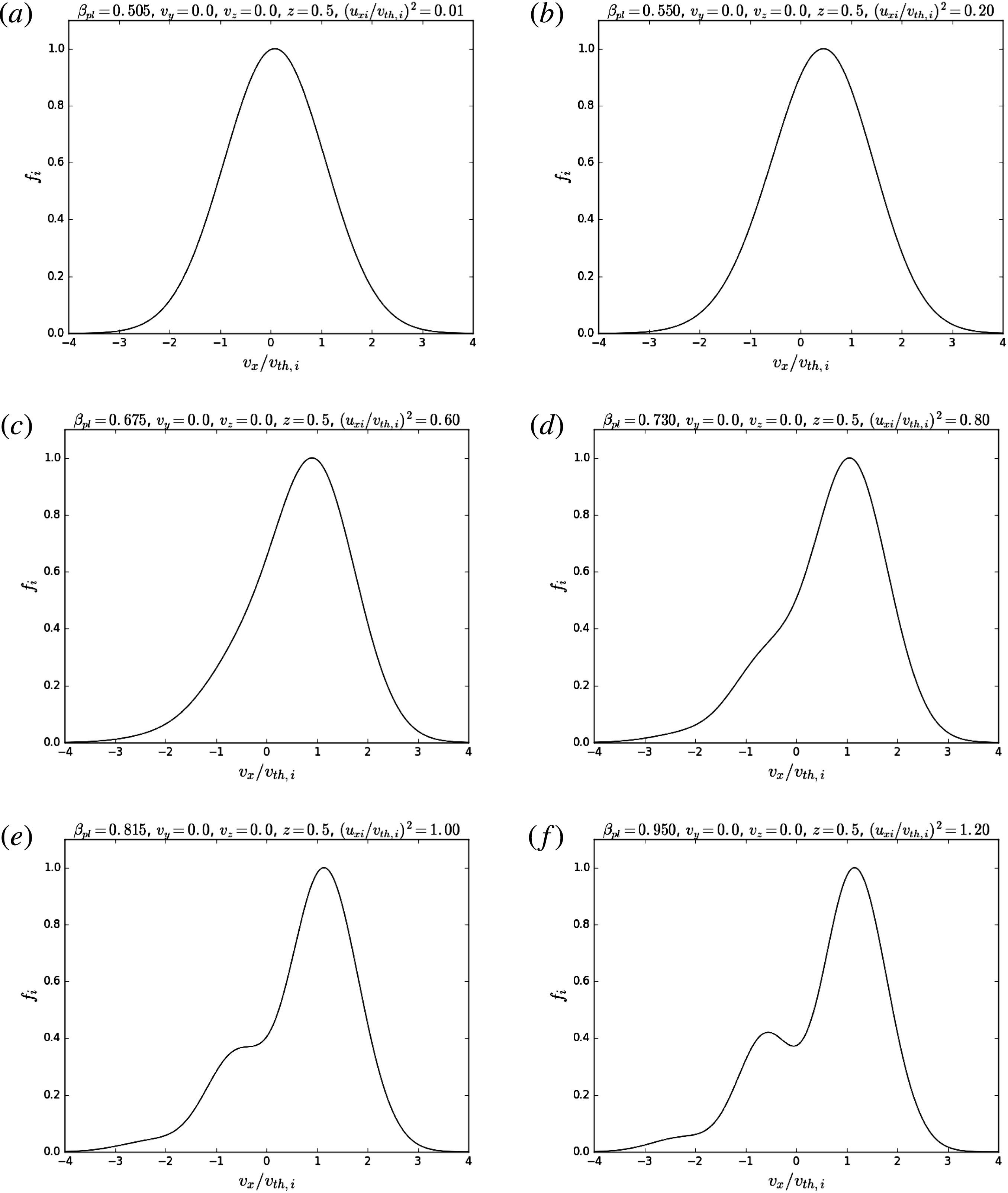
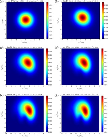
In this section, we will show some illustrative plots of the quadratic DF (4.14) for different parameter values. Figures 1 and 2 show plots of the ion DF in the
 $v_{x}$
-direction (with
 $v_{y}=0$
) for various values of
 $u_{xi}/v_{th,i}$
, for
 $z=0$
(figure 1) and
 $z=0.5$
(figure 2). In each case, we have adjusted
 $b$
according to the condition (4.21) for positivity of the DF, and hence the plasma beta is different in each plot. The DFs are normalised to have a maximum value of one in each case. Note that, for negative values of
 $z$
, the DF has the opposite symmetry from that for positive
 $z$
values with respect to
 $v_{x}=0$
(i.e. the DF is symmetric under the transformation
 $v_{x}\rightarrow -v_{x}$
,
 $z\rightarrow -z$
) and so we only show plots for a positive value of
 $z$
(
 $z=0.5$
) to illustrate the behaviour of the DF away from
 $z=0$
.
Plots of the ion DF (4.14) in the
 $v_{x}$
-direction (with
 $v_{y}=v_{z}=z=0$
) for various values of
 $u_{xi}/v_{th,i}$
and, hence, the plasma beta. The DFs are normalised to have a maximum value of one in each case.

Plots of the ion DF (4.14) in the
 $v_{x}$
-direction (with
 $v_{y}=v_{z}$
and
 $z=0.5$
) for various values of
 $u_{xi}/v_{th,i}$
and, hence, the plasma beta. The DFs are normalised to have a maximum value of one in each case.

We see that, for small values of
 $u_{xi}/v_{th,i}$
(and hence
 $\unicode[STIX]{x1D6FD}_{\text{pl}}$
), the DF is single peaked but, as
 $u_{xi}/v_{th,i}$
is increased, multiple maxima eventually appear in the DF, and these are more pronounced at
 $z=0$
than at
 $z=0.5$
. Due to the condition (4.21) on
 $b$
, however, these multiple maxima appear for
 $\unicode[STIX]{x1D6FD}_{\text{pl}}$
values only modestly below one. For the parameter values considered by Neukirch et al. (Reference Neukirch, Wilson and Allanson2018), only single maxima were found. Since this work was carried out, however, we have found that we can take less restrictive values of
 $u_{xi}^{2}/v_{th,i}^{2}$
and still have positive DFs over the whole phase space. We also note that the quadratic DF can have more pronounced multiple maxima for higher values of
 $u_{xi}/v_{th,i}$
. We do not focus on such cases, however, since they occur at increasingly high values of the plasma beta due to the condition (4.21). We have only plotted ion DFs here, since the electron DFs are single peaked for the given parameter values (due to (4.22), the values of
 $u_{xe}^{2}/v_{th,e}^{2}$
will be very small unless we take a very large value of
 $T_{e}/T_{i}$
).
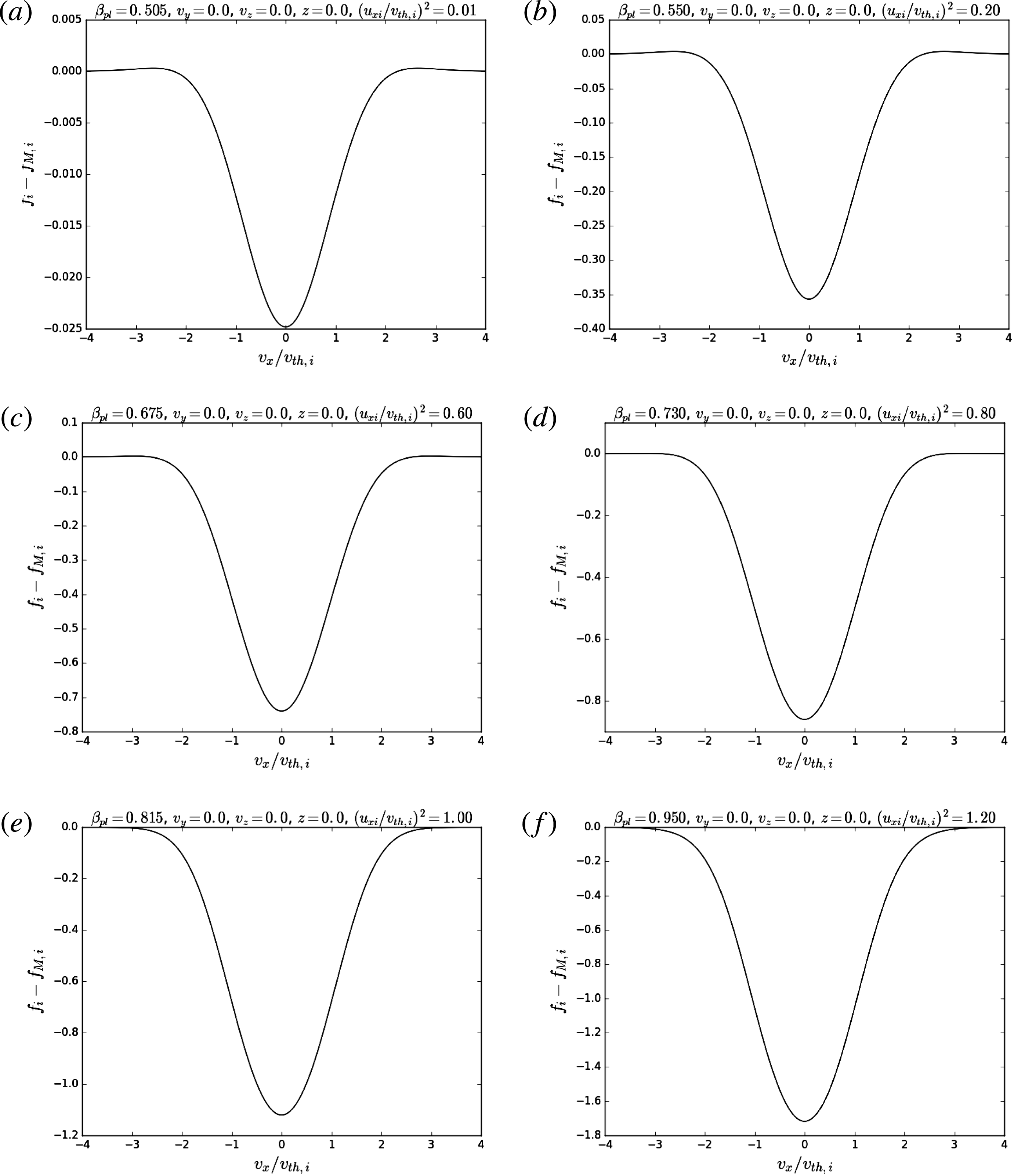
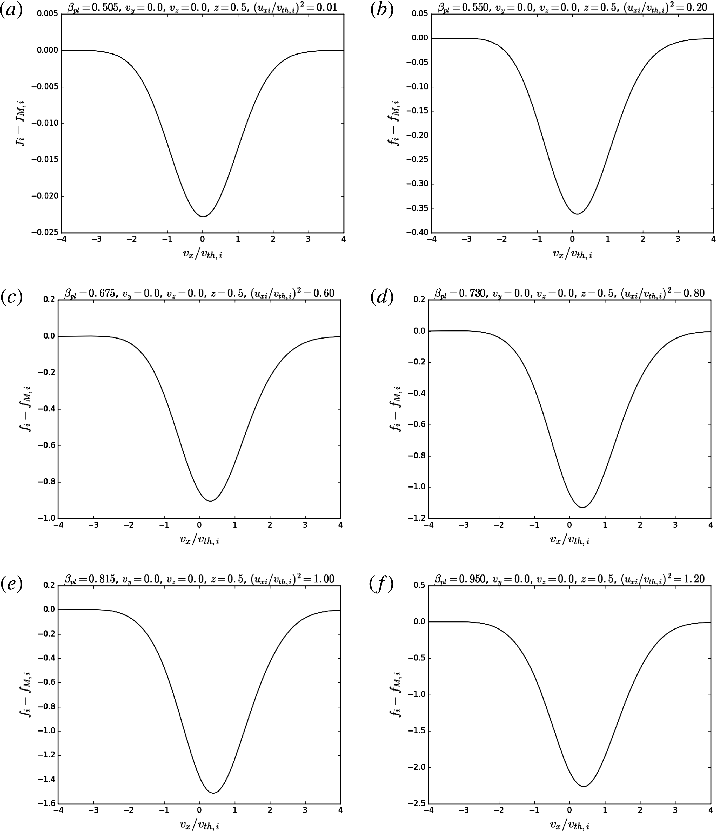
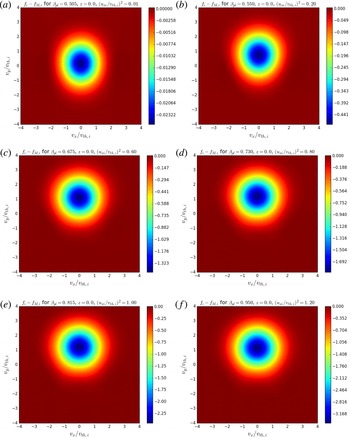
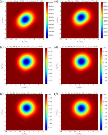
Figures 3 (
 $z=0$
) and 4 (
 $z=0.5$
) show, for the same values of
 $u_{xi}/v_{th,i}$
and
 $\unicode[STIX]{x1D6FD}_{\text{pl}}$
as in figures 1 and 2, plots of the difference between the quadratic ion DF and the Maxwellian DF given by
 $$\begin{eqnarray}f_{M,i}=\frac{n_{0,M}}{(\sqrt{2\unicode[STIX]{x03C0}}v_{th,s})^{3}}\exp \left[-\frac{(\boldsymbol{v}-\boldsymbol{V}_{s})}{2v_{th,s}^{2}}^{2}\right],\end{eqnarray}$$
where the non-vanishing components of the average velocity
 $\boldsymbol{V}_{s}$
are given in (4.17) and (4.18), and
 $n_{0,M}=n_{0}(1/2+b)^{2}$
so that the density, current density and pressure (
 $\unicode[STIX]{x1D617}_{zz}$
) calculated from the Maxwellian DF match with those calculated from the DF (4.14). We see from figures 3 and 4 that the deviation of the DFs from the Maxwellian DF (4.26) is much larger than might be assumed from figures 1 and 2. For increasing
 $u_{xi}/v_{th,i}$
, there is an increase in the difference between the quadratic DF and the Maxwellian DF, which is to be expected, due to the appearance of multiple peaks in the DF for these parameters. We also note that, for the parameter values shown, the electron DFs are closer to Maxwellian than the ion DFs, due to the much smaller values of
 $u_{xe}/v_{th,e}$
for physically reasonable values of
 $T_{e}/T_{i}$
.
Plots of
 $f_{i}-f_{M,i}$
in the
 $v_{x}$
-direction (with
 $v_{y}=v_{z}=z=0$
) for various values of
 $u_{xi}/v_{th,i}$
and, hence, the plasma beta.

Plots of
 $f_{i}-f_{M,i}$
in the
 $v_{x}$
-direction (with
 $v_{y}=v_{z}$
and
 $z=0.5$
) for various values of
 $u_{xi}/v_{th,i}$
and, hence, the plasma beta.

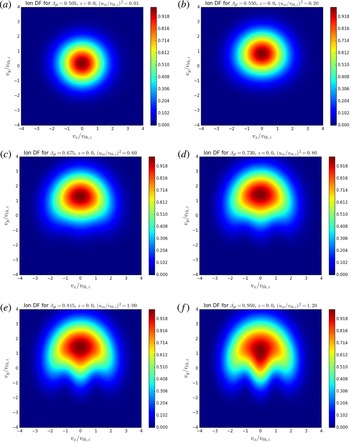
Figures 5 (
 $z=0$
) and 6 (
 $z=0.5$
) show contour plots of the ion DF in the
 $v_{x}$
–
 $v_{y}$
-plane (for
 $v_{z}=0$
), for the same parameter values as before. The values for
 $v_{y}=0$
do not match up between the two figures, however, since the normalisation is different (here we have normalised so that the maximum value over the plane is one). Again, we can see the multiple peaks in the
 $v_{x}$
-direction, this time for a range of
 $v_{y}$
values in each case, and note that for these parameters the DF is single peaked in the
 $v_{y}$
-direction. As before, the electron DFs will be single peaked (and closer to Maxwellian) for these parameters due to the small values of
 $u_{xe}^{2}/v_{th,e}^{2}$
.
Contour plots of the ion DF (4.14) in the
 $v_{x}$
–
 $v_{y}$
-plane (
 $z=0$
) for various values of
 $u_{xi}/v_{th,i}$
and, hence, the plasma beta. The DFs are normalised to have a maximum value of one in each case.

Contour plots of the ion DF (4.14) in the
 $v_{x}$
–
 $v_{y}$
-plane (
 $z=0.5$
) for various values of
 $u_{xi}/v_{th,i}$
and, hence, the plasma beta. The DFs are normalised to have a maximum value of one in each case.

Figures 7 (
 $z=0$
) and 8 (
 $z=0.5$
) show contour plots of
 $f_{i}-f_{M,i}$
in the
 $v_{x}$
–
 $v_{y}$
-plane (for
 $v_{z}=0$
), for the same parameter values as before. Again, we see that there is a substantial difference between the quadratic DF and the Maxwellian, even for small values of
 $u_{xi}/v_{th,i}$
when the DF looks close to Maxwellian. This difference is again seen to get larger as we increase
 $u_{xi}/v_{th,i}$
.
Contour plots of
 $f_{i}-f_{M,i}$
in the
 $v_{x}$
–
 $v_{y}$
-plane (
 $z=0$
) for the parameter values from figure 5.

Contour plots of
 $f_{i}-f_{M,i}$
in the
 $v_{x}$
–
 $v_{y}$
-plane (
 $z=0.5$
) for the parameter values from figure 5.

We will now compare the plots of the quadratic DF with the examples given by Allanson et al. (Reference Allanson, Neukirch, Wilson and Troscheit2015), in which only single-peaked DFs are found. To do this, we define the magnetisation parameter,
 $\unicode[STIX]{x1D6FF}_{s}$
, as
 $$\begin{eqnarray}\unicode[STIX]{x1D6FF}_{s}=\frac{m_{s}v_{th,s}}{eB_{0}L},\end{eqnarray}$$
i.e. the ratio between the species gyroradius,
 $\unicode[STIX]{x1D70C}_{s}=v_{th,s}/\unicode[STIX]{x1D6FA}_{s}$
(for
 $\unicode[STIX]{x1D6FA}_{s}=eB_{0}/m_{s}$
the species gyrofrequency) and the current sheet half-thickness,
 $L$
. By using (4.5), we can derive the following relation between
 $u_{xs}$
and
 $\unicode[STIX]{x1D6FF}_{s}$
,
 $$\begin{eqnarray}\frac{|u_{xs}|}{v_{th,s}}=2\unicode[STIX]{x1D6FF}_{s}.\end{eqnarray}$$
We can compare plots of the quadratic DF with the results of Allanson et al. (Reference Allanson, Neukirch, Wilson and Troscheit2015) by using the same values of
 $\unicode[STIX]{x1D6FF}_{s}$
and
 $\unicode[STIX]{x1D6FD}_{\text{pl}}$
(
 $\unicode[STIX]{x1D6FF}_{s}=0.15$
,
 $\unicode[STIX]{x1D6FD}_{\text{pl}}=0.85$
). These are shown in figures 9 (contour plots of
 $f_{i}$
), 10 (contour plots of
 $f_{i}-f_{M,i}$
), 11 (line plots of
 $f_{i}/f_{M,i}$
in the
 $v_{x}$
-direction) and 12 (line plots of
 $f_{i}/f_{M,i}$
in the
 $v_{y}$
-direction). The
 $z$
values shown are
 $z=0$
and
 $z=1$
, to match those chosen by Allanson et al. (Reference Allanson, Neukirch, Wilson and Troscheit2015). It is important to note that the Maxwellian DF used for comparison is normalised differently here than it is in the work by Allanson et al. (Reference Allanson, Neukirch, Wilson and Troscheit2015) (so that the appropriate velocity moments are reproduced), but it is still useful to compare the departure from the respective Maxwellian DF in each case. The figures show that the quadratic DF (4.14) is single peaked for these parameter values, and that there is a significant departure from the Maxwellian DF, which has a different profile than that found by Allanson et al. (Reference Allanson, Neukirch, Wilson and Troscheit2015). In the
 $v_{x}$
-direction, we see that the profile and values of
 $f_{i}/f_{M,i}$
for
 $z=0$
are not too different that that found by Allanson et al. (Reference Allanson, Neukirch, Wilson and Troscheit2015), but for
 $z=1$
the difference is much more noticeable. In the
 $v_{y}$
-direction, the profiles of
 $f_{i}/f_{M,i}$
are qualitatively similar to those found by Allanson et al. (Reference Allanson, Neukirch, Wilson and Troscheit2015), but the values are significantly smaller in the quadratic case.
Contour plots of the ion DF (4.14) in the
 $v_{x}$
–
 $v_{y}$
-plane (
 $v_{z}=0$
) for the parameters used by Allanson et al. (Reference Allanson, Neukirch, Wilson and Troscheit2015), for (a)
 $z=0$
and (b)
 $z=1.0$
.

Contour plots of
 $f_{i}-f_{M,i}$
in the
 $v_{x}$
–
 $v_{y}$
-plane (
 $v_{z}=0$
) for the parameters used by Allanson et al. (Reference Allanson, Neukirch, Wilson and Troscheit2015), for (a)
 $z=0$
and (b)
 $z=1.0$
.

Plots of
 $f_{i}/f_{M,i}$
in the
 $v_{x}$
-direction for the parameters used by Allanson et al. (Reference Allanson, Neukirch, Wilson and Troscheit2015), for (a)
 $z=0$
and (b)
 $z=1.0$
.

Plots of
 $f_{i}/f_{M,i}$
in the
 $v_{y}$
-direction for the parameters used by Allanson et al. (Reference Allanson, Neukirch, Wilson and Troscheit2015), for (a)
 $z=0$
and (b)
 $z=1.0$
.

Since, for the quadratic DF case (
 $N=2$
), the lowest obtainable value of
 $\unicode[STIX]{x1D6FD}_{\text{pl}}$
is
 $1/2$
, we cannot compare our results with those of Allanson et al. (Reference Allanson, Neukirch, Troscheit and Wilson2016a
), in which
 $\unicode[STIX]{x1D6FD}_{\text{pl}}=0.05$
is used (for our method,
 $N\geqslant 20$
would be necessary for a comparison). In that work, it was suggested that multiple maxima may occur for large values of
 $\unicode[STIX]{x1D6FF}_{s}/\unicode[STIX]{x1D6FD}_{\text{pl}}$
, which corresponds to large
 $\unicode[STIX]{x1D6FF}_{s}$
here (due to the different definition of
 $u_{s}$
as discussed above). For such parameter ranges, however, numerical convergence could not be achieved for the Hermite polynomial sums, and so the behaviour of the DFs could not be investigated. Looking at the quadratic DF for such parameter ranges, we see that multiple maxima occur, i.e. as
 $u_{xs}$
(
 $\unicode[STIX]{x1D6FF}_{s}$
) is increased. While this is not proof of the correctness of the conjecture made by Allanson et al. (Reference Allanson, Neukirch, Troscheit and Wilson2016a
), it is interesting that we now at least have an example for DFs exhibiting multiple maxima in the suggested parameter regime.
The presence of multiple maxima in the DFs raises the question of whether they could be microscopically unstable. A full stability analysis is beyond the scope of this paper but, to get an indication of stability, we have applied the Penrose criterion (e.g. Krall & Trivelpiece Reference Krall and Trivelpiece1973) locally to the DFs, treating
 $z$
as a parameter (see appendix E). Although this is not expected to provide a complete assessment of the stability properties of the DFs, it is reassuring that all the cases we investigated with
 $\unicode[STIX]{x1D6FD}_{\text{pl}}<1$
and multiple maxima were found to be stable according to the Penrose criterion.
5 Summary and conclusions
Up to now, with the exception of the linear force-free case (Sestero Reference Sestero1967; Bobrova et al.
Reference Bobrova, Bulanov, Sakai and Sugiyama2001), only one single example of an explicitly known DF for collisionless force-free current sheets allowing plasma beta values smaller than one was known (Allanson et al.
Reference Allanson, Neukirch, Wilson and Troscheit2015, Reference Allanson, Neukirch, Troscheit and Wilson2016a
). This DF can only be expressed as an infinite sum of Hermite functions with very slow convergence, which makes it cumbersome to use in practice. In this paper, we have presented a method that allows us to find further equilibrium DFs for force-free current sheets with a plasma beta smaller than one, but which consist of a finite number of terms and are, therefore, easier to use. As in the work by Allanson et al. (Reference Allanson, Neukirch, Wilson and Troscheit2015, Reference Allanson, Neukirch, Troscheit and Wilson2016a
), the method is based on a transformation of the pressure, as suggested by Harrison & Neukirch (Reference Harrison and Neukirch2009b
). The transformation used in this paper is an integer power (
 $N$
) of the original pressure, allowing in principle for a reduction of the plasma beta by a factor of
 $1/N$
.
For the example of the force-free Harris sheet, we have derived the corresponding DFs for each
 $N$
in closed form and, to provide an illustrative example, have given a detailed analysis of the quadratic case (
 $N=2$
), giving a much more comprehensive discussion than that previously given by Neukirch et al. (Reference Neukirch, Wilson and Allanson2018). An interesting aspect of this detailed analysis is that the conditions on the parameters for the quadratic case are much less restrictive than assumed by Neukirch et al. (Reference Neukirch, Wilson and Allanson2018). These less restrictive conditions allow us to achieve multi-peaked DFs that give rise to a plasma beta of lower than one, whereas, for the parameter range considered by Neukirch et al. (Reference Neukirch, Wilson and Allanson2018), only single-peaked DFs were found. In the work by Allanson et al. (Reference Allanson, Neukirch, Wilson and Troscheit2015, Reference Allanson, Neukirch, Troscheit and Wilson2016a
), only single-peaked DFs were found, which is an obvious difference between the two models. It must be emphasised, however, that in the work by Allanson et al. (Reference Allanson, Neukirch, Wilson and Troscheit2015, Reference Allanson, Neukirch, Troscheit and Wilson2016a
), the full parameter range could not be explored since numerical convergence of the infinite sums could not always be achieved. For the parameters used by Allanson et al. (Reference Allanson, Neukirch, Wilson and Troscheit2015), the new DFs presented in this paper are single peaked.
In the quadratic case example, the plasma beta is bounded from below by
 $1/2$
, which is a disadvantage compared with the DFs found by Allanson et al. (Reference Allanson, Neukirch, Wilson and Troscheit2015, Reference Allanson, Neukirch, Troscheit and Wilson2016a
), in which the plasma beta could be arbitrarily small. However, the minimum value of the plasma beta can in principle be made smaller by making the power
 $N$
in the transformation larger. As demonstrated in this paper, for the general
 $N$
case, it is possible to derive both DFs and conditions on the parameters that ensure strict neutrality and consistency between the macroscopic and microscopic parameters of the equilibrium. The conditions for the positivity of the DF will have to be considered along the same lines as presented in this paper for the quadratic case, but on a case-by-case basis.
Acknowledgements
The authors would like to thank the anonymous referees, whose comments have helped to improve this manuscript. We acknowledge the support of the Science and Technology Facilities Council via the consolidated grants ST/K000950/1 and ST/N000609/1 and the doctoral training grant ST/K502327/1 (O.A.), and the Natural Environment Research Council via grant no. NE/P017274/1 (Rad-Sat) (O.A.). F.W. and T.N. would also like to thank the University of St Andrews for general financial support.
Appendix A. The ‘full’ plasma beta for the quadratic case
As stated in § 3, throughout this paper we have defined the plasma beta as
 $\unicode[STIX]{x1D6FD}_{\text{pl}}=\unicode[STIX]{x1D617}_{zz}/(B^{2}/(2\unicode[STIX]{x1D707}_{0}))$
, for
 $\unicode[STIX]{x1D617}_{zz}$
the
 $zz$
-component of the pressure tensor. It may also be of interest, however, to investigate the effect of the pressure transformation on the quantity
 $\bar{\unicode[STIX]{x1D6FD}}_{\text{pl}}=P/(B^{2}/(2\unicode[STIX]{x1D707}_{0}))$
, where
 $P=(\unicode[STIX]{x1D617}_{xx}+\unicode[STIX]{x1D617}_{yy}+\unicode[STIX]{x1D617}_{zz})/3$
, since this is the more conventional definition of the plasma beta. We will illustrate this for the quadratic pressure transformation. Using the definitions of the diagonal pressure tensor components,
 $P$
can be calculated as
 $$\begin{eqnarray}\displaystyle P=\frac{1}{3}\mathop{\sum }_{s}m_{s}\left(\int \boldsymbol{v}^{2}f_{s}\,\text{d}^{3}v-n_{s}\boldsymbol{V}_{s}^{2}\right). & & \displaystyle\end{eqnarray}$$
Using (4.7), (4.16), (4.17) and (4.18), and substituting the DF (4.14) into (A 1) gives, for the quadratic case,
 $$\begin{eqnarray}\displaystyle \bar{\unicode[STIX]{x1D6FD}}_{\text{pl}} & = & \displaystyle \frac{1}{2}\left(\frac{1}{2}+b\right)+\frac{1}{3}\frac{\unicode[STIX]{x1D6FD}_{e}}{\unicode[STIX]{x1D6FD}_{e}+\unicode[STIX]{x1D6FD}_{i}}\left(1+\frac{T_{e}^{2}}{T_{i}^{2}}\frac{m_{e}}{m_{i}}\right)\frac{u_{xi}^{2}}{v_{th,i}^{2}}\left(\frac{4b\,\text{sech}^{2}(z/L)}{1+2b}-2\right).\end{eqnarray}$$
An equivalent expression can be derived for Harrison and Neukirch’s DF for the untransformed pressure (Neukirch et al. Reference Neukirch, Wilson and Harrison2009; Harrison & Neukirch Reference Harrison and Neukirch2009a ) as
 $$\begin{eqnarray}\displaystyle \bar{\unicode[STIX]{x1D6FD}}_{\text{pl},H\& N}=\left(\frac{1}{2}+b\right)+\frac{1}{3}\frac{\unicode[STIX]{x1D6FD}_{e}}{\unicode[STIX]{x1D6FD}_{e}+\unicode[STIX]{x1D6FD}_{i}}\left(1+\frac{T_{e}^{2}}{T_{i}^{2}}\frac{m_{e}}{m_{i}}\right)\frac{u_{xi}^{2}}{v_{th,i}^{2}}\left(\frac{4b\,\text{sech}^{2}(z/L)}{1+2b}-\frac{1}{2}\right). & & \displaystyle\end{eqnarray}$$
Clearly, the quadratic pressure transformation has also had the effect of reducing
 $\bar{\unicode[STIX]{x1D6FD}}_{\text{pl}}$
. In the limit
 $u_{xi}\rightarrow 0$
, we have
 $\bar{\unicode[STIX]{x1D6FD}}_{\text{pl}}=\unicode[STIX]{x1D6FD}_{\text{pl}}$
in each case.
Appendix B. The plasma beta for summative pressure functions
It can be seen from various current sheet models discussed in the literature (e.g. Channell Reference Channell1976; Attico & Pegoraro Reference Attico and Pegoraro1999; Neukirch et al. Reference Neukirch, Wilson and Harrison2009; Harrison & Neukirch Reference Harrison and Neukirch2009a ; Wilson & Neukirch Reference Wilson and Neukirch2011; Abraham-Shrauner Reference Abraham-Shrauner2013; Kolotkov et al. Reference Kolotkov, Vasko and Nakariakov2015; Wilson et al. Reference Wilson, Neukirch and Allanson2017) that, if the pressure function is of a summative form in terms of its dependence on the vector potential components, i.e.
 $$\begin{eqnarray}P(A_{x},A_{y})=P_{1}(A_{x})+P_{2}(A_{y}),\end{eqnarray}$$
then the plasma beta is constrained to be at least one. This has been considered in a more general sense by Allanson (Reference Allanson2017); in this appendix, we will summarise the discussion given therein.
Firstly, for summative pressure functions of the form in (B 1), the force balance equation for force-free fields, given by
 $$\begin{eqnarray}\unicode[STIX]{x1D617}_{zz}(A_{x},A_{y})+\frac{B_{0}^{2}}{2\unicode[STIX]{x1D707}_{0}}=P_{T},\end{eqnarray}$$
can be split into the two equations
 $$\begin{eqnarray}\displaystyle \left.\begin{array}{@{}c@{}}\displaystyle P_{1}(A_{x})+\frac{1}{2\unicode[STIX]{x1D707}_{0}}B_{y}^{2}(A_{x})=P_{T1},\\ \displaystyle P_{2}(A_{y})+\frac{1}{2\unicode[STIX]{x1D707}_{0}}B_{x}^{2}(A_{y})=P_{T2},\end{array}\right\} & & \displaystyle\end{eqnarray}$$
where
 $P_{T1}+P_{T2}=P_{T}$
is the total pressure (for constants
 $P_{T1}$
and
 $P_{T2}$
).
Secondly, as discussed by Bobrova et al. (Reference Bobrova, Bulanov, Sakai and Sugiyama2001) and Vekstein, Bobrova & Bulanov (Reference Vekstein, Bobrova and Bulanov2002), all 1-D force-free magnetic fields can be written in the general form
 $$\begin{eqnarray}\boldsymbol{B}(z)=B_{0}(\cos (S(z)),\sin (S(z)),0),\end{eqnarray}$$
where
 $S(z)=\int \unicode[STIX]{x1D6FC}(z)\,\text{d}z$
, with
 $\unicode[STIX]{x1D6FC}$
the force-free parameter as discussed in § 1. For linear force-free fields (Sestero Reference Sestero1967; Channell Reference Channell1976; Attico & Pegoraro Reference Attico and Pegoraro1999; Bobrova et al.
Reference Bobrova, Bulanov, Sakai and Sugiyama2001), the function
 $S(z)$
must be a linear function of
 $z$
, whereas for nonlinear force-free fields the function
 $S(z)$
can, in principle, be any differentiable function.
We will now assume that
(i)
$P_{1}(A_{x})\geqslant 0$
and
$P_{2}(A_{y})\geqslant 0$
,(ii) there exist points
$z=z_{1}$
,
$z=z_{2}$
such that (B 5a-d )$$\begin{eqnarray}\sin ^{2}(S(z_{1}))=1,\quad \cos ^{2}(S(z_{1}))=0,\quad \sin ^{2}(S(z_{2}))=0,\quad \cos ^{2}(S(z_{2}))=1.\end{eqnarray}$$


Assumption (i) can be justified by considering the inverse problem defined by (2.5), in which the dependence of
 $\unicode[STIX]{x1D617}_{zz}$
on
 $A_{x}$
and
 $A_{y}$
is tied to the dependence of the DF of
 $p_{xs}$
and
 $p_{ys}$
, respectively. Since the DF must be positive with respect to the independent variation of
 $p_{xs}$
and
 $p_{ys}$
, it follows that
 $\unicode[STIX]{x1D617}_{zz}$
must be positive with respect to independent variations of
 $A_{x}$
and
 $A_{y}$
.
Assumption (ii) is always true for a linear force-free field, since
 $S(z)$
is a linear function. It will also hold for a particular class of nonlinear force-free fields, in which one of the magnetic field components goes through zero, and the other tends to zero at
 $\pm \infty$
. The force-free Harris sheet (1.4) is an example of such a magnetic field profile. Combining the assumptions made above, we have that
 $$\begin{eqnarray}\displaystyle & \displaystyle P_{T1}=P_{1}(A_{x}(z_{1}))+\frac{B_{0}^{2}}{2\unicode[STIX]{x1D707}_{0}}\sin ^{2}(S(z_{1}))\geqslant \frac{B_{0}^{2}}{2\unicode[STIX]{x1D707}_{0}}, & \displaystyle\end{eqnarray}$$
 $$\begin{eqnarray}\displaystyle & \displaystyle P_{T2}=P_{2}(A_{y}(z_{2}))+\frac{B_{0}^{2}}{2\unicode[STIX]{x1D707}_{0}}\cos ^{2}(S(z_{2}))\geqslant \frac{B_{0}^{2}}{2\unicode[STIX]{x1D707}_{0}}, & \displaystyle\end{eqnarray}$$
for the particular points
 $z_{1}$
and
 $z_{2}$
defined above. However, since
 $\unicode[STIX]{x1D617}_{zz}$
is constant, and
 $P_{T1}$
and
 $P_{T2}$
are independent of each other through separation of variables, the conditions in (B 6) must be valid for all values of
 $z$
. This fact, together with the (B 3), gives
 $$\begin{eqnarray}P_{T}=P_{T1}+P_{T2}\geqslant 2\frac{B_{0}^{2}}{2\unicode[STIX]{x1D707}_{0}}\Rightarrow P_{1}(A_{x})+P_{2}(A_{y})+\frac{B_{0}^{2}}{2\unicode[STIX]{x1D707}_{0}}\geqslant 2\frac{B_{0}^{2}}{2\unicode[STIX]{x1D707}_{0}}.\end{eqnarray}$$
Finally, dividing through by the magnetic pressure,
 $B_{0}^{2}/(2\unicode[STIX]{x1D707}_{0})$
, gives
 $$\begin{eqnarray}\unicode[STIX]{x1D6FD}_{\text{pl}}+1\geqslant 2\Rightarrow \unicode[STIX]{x1D6FD}_{\text{pl}}\geqslant 1.\end{eqnarray}$$
This discussion demonstrates that, for linear force-free fields and certain types of nonlinear force-free fields, the plasma beta is constrained to be at least one whenever the pressure function is assumed to have a summative form.
Appendix C. Distribution functions for a general
$N$

The pressure function (3.12) can be written in the expanded form
 $$\begin{eqnarray}\displaystyle \bar{P}_{zz} & = & \displaystyle \frac{B_{0}^{2}}{2\unicode[STIX]{x1D707}_{0}}\frac{(1/2+b)^{1-N}}{N}\mathop{\sum }_{k=0}^{N}\mathop{\sum }_{l=0}^{N-k}\binom{N}{k}\binom{N-k}{l}\frac{b^{l}}{2^{N-k-l}}\cos ^{N-k-l}\left(\frac{2A_{x}}{B_{0}L}\right)\exp \left(\frac{2kA_{y}}{B_{0}L}\right).\nonumber\\ \displaystyle & & \displaystyle\end{eqnarray}$$
The function (C 1) can be substituted into (2.5), which can then be solved (e.g. by using Fourier/Weierstrass transforms) to give the DF as
 $$\begin{eqnarray}\displaystyle f_{s}(H_{s},p_{xs},p_{ys}) & = & \displaystyle f_{0s}\text{e}^{-\unicode[STIX]{x1D6FD}_{s}H_{s}}\mathop{\sum }_{k=0}^{N}\mathop{\sum }_{l=0}^{N-k}\mathop{\sum }_{m=0}^{N-k-l}\binom{N}{k}\binom{N-k}{l}\binom{N-k-l}{m}\frac{b^{l}}{2^{2(N-k-l)}}\nonumber\\ \displaystyle & & \displaystyle \times \,\text{e}^{[(2m-(N-k-l))^{2}u_{xs}^{2}-k^{2}u_{ys}^{2}]/2v_{th,s}^{2}}\text{e}^{-\text{i}(2m-(N-k-l))\unicode[STIX]{x1D6FD}_{s}u_{xs}p_{xs}}\text{e}^{k\unicode[STIX]{x1D6FD}_{s}u_{ys}p_{ys}},\nonumber\\ \displaystyle & & \displaystyle\end{eqnarray}$$
where we have introduced the constant microscopic parameters
 $f_{0s}$
,
 $u_{xs}$
and
 $u_{ys}$
. The moments of this DF can be calculated as demonstrated in § 4 for the
 $N=2$
case, giving conditions between the microscopic and macroscopic parameters of the equilibrium.
For a physically meaningful solution, we need to ensure that
 $f_{s}\geqslant 0$
; this can be satisfied for
 $N=2$
, as is shown in appendix D. For
 $N>2$
, one would proceed along the same lines as for
 $N=2$
, but the calculation becomes more involved.
Appendix D. Positivity of the quadratic distribution function
In this appendix, we will show that a necessary and sufficient condition for positivity of the quadratic DF (4.14) over the whole phase space is
 $$\begin{eqnarray}b\geqslant \frac{\text{e}^{\bar{u}_{xs}^{2}/2}}{2\sqrt{2}}(\text{e}^{\bar{u}_{xs}^{2}}+1)^{1/2}.\end{eqnarray}$$
Positivity of the DF requires positivity of the function
 $$\begin{eqnarray}\displaystyle g_{s}(X,Y)={\textstyle \frac{1}{8}}\text{e}^{2\unicode[STIX]{x1D6FC}}\cos (2X)+\text{e}^{-2\unicode[STIX]{x1D6FC}}\text{e}^{2Y}+\text{e}^{Y}\cos X+b\text{e}^{\unicode[STIX]{x1D6FC}/2}\cos X+2b\text{e}^{-\unicode[STIX]{x1D6FC}/2}\text{e}^{Y}+b^{2}+{\textstyle \frac{1}{8}}, & & \displaystyle \nonumber\\ \displaystyle & & \displaystyle\end{eqnarray}$$
over the whole phase space, where
 $X=\unicode[STIX]{x1D6FD}_{s}u_{xs}p_{xs}$
,
 $Y=\unicode[STIX]{x1D6FD}_{s}u_{ys}p_{ys}$
and
 $\unicode[STIX]{x1D6FC}=\bar{u}_{xs}^{2}$
(note that
 $X$
,
 $Y$
and
 $\unicode[STIX]{x1D6FC}$
are species dependent but we do not show
 $s$
subscripts for notational convenience). Using that fact that
 $\cos (2X)=2\cos ^{2}X-1$
and writing
 $$\begin{eqnarray}\displaystyle {\textstyle \frac{1}{4}}\text{e}^{2\unicode[STIX]{x1D6FC}}\cos ^{2}X+\text{e}^{Y}\cos X={\textstyle \frac{1}{4}}\text{e}^{2\unicode[STIX]{x1D6FC}}(\cos X+2\text{e}^{-2\unicode[STIX]{x1D6FC}}\text{e}^{Y})^{2}-\text{e}^{-2\unicode[STIX]{x1D6FC}}\text{e}^{2Y}, & & \displaystyle\end{eqnarray}$$
we see that
 $g_{s}\geqslant 0$
requires
 $$\begin{eqnarray}{\textstyle \frac{1}{4}}\text{e}^{2\unicode[STIX]{x1D6FC}}(\cos X+2\text{e}^{-2\unicode[STIX]{x1D6FC}}\text{e}^{Y})^{2}+(2\text{e}^{-\unicode[STIX]{x1D6FC}/2}\text{e}^{Y}+\text{e}^{\unicode[STIX]{x1D6FC}/2}\cos X)b+b^{2}+{\textstyle \frac{1}{8}}(1-\text{e}^{2\unicode[STIX]{x1D6FC}})\geqslant 0.\end{eqnarray}$$
D.1
$p_{ys}$
-direction

We first consider the
 $p_{ys}$
-direction (i.e. the
 $Y$
-direction) and look to minimise
 $g_{s}$
with respect to
 $\unicode[STIX]{x1D709}=\text{e}^{Y}$
. We have
 $$\begin{eqnarray}\frac{\unicode[STIX]{x2202}g_{s}}{\unicode[STIX]{x2202}\unicode[STIX]{x1D709}}=2\text{e}^{-2\unicode[STIX]{x1D6FC}}\unicode[STIX]{x1D709}+\cos X+2b\text{e}^{-\unicode[STIX]{x1D6FC}/2},\end{eqnarray}$$
which vanishes for
 $$\begin{eqnarray}\unicode[STIX]{x1D709}=\unicode[STIX]{x1D709}_{min}=-\frac{\text{e}^{2\unicode[STIX]{x1D6FC}}}{2}(\cos X+2b\text{e}^{-\unicode[STIX]{x1D6FC}/2}),\end{eqnarray}$$
i.e. when
 $Y=Y_{min}=\ln |\unicode[STIX]{x1D709}_{min}|$
. This gives
 $$\begin{eqnarray}\displaystyle g_{s}(X,Y_{min})=-(\text{e}^{\unicode[STIX]{x1D6FC}}-1)b^{2}-\text{e}^{\unicode[STIX]{x1D6FC}/2}\cos X(\text{e}^{\unicode[STIX]{x1D6FC}}-1)b-{\textstyle \frac{1}{8}}(\text{e}^{2\unicode[STIX]{x1D6FC}}-1), & & \displaystyle\end{eqnarray}$$
which is a minimum since
 $$\begin{eqnarray}\left.\frac{\unicode[STIX]{x2202}^{2}g_{s}}{\unicode[STIX]{x2202}\unicode[STIX]{x1D709}^{2}}\right|_{\unicode[STIX]{x1D709}=\unicode[STIX]{x1D709}_{min}}=2\text{e}^{-2\unicode[STIX]{x1D6FC}}>0.\end{eqnarray}$$
We require
 $g_{s}(X,Y_{min})>0$
. If we assume that
 $\unicode[STIX]{x1D709}_{min}>0$
, i.e. that
 $b<-\text{e}^{\unicode[STIX]{x1D6FC}/2}/2$
, we see that
 $g_{s}(X,Y_{min})>0$
cannot be satisfied for all
 $X$
; the first and third terms on the right-hand side of (D 7) are always negative (because
 $\unicode[STIX]{x1D6FC}\geqslant 0$
). The second term can be positive or negative for some range of
 $X$
values, and so the right-hand side cannot be positive for all
 $X$
. Note also that
 $b<-1/2$
would lead to a negative pressure through equation (4.2), and so it would not make sense if this parameter range were found to give rise to positive DFs over the whole phase space. We assume, therefore, that
 $\unicode[STIX]{x1D709}_{min}\leqslant 0$
, which gives
 $b\geqslant \text{e}^{\unicode[STIX]{x1D6FC}/2}/2$
. However,
 $\unicode[STIX]{x1D709}$
must be at least zero, since
 $\unicode[STIX]{x1D709}=\text{e}^{Y}$
. Therefore, since
 $g_{s}$
is an increasing function of
 $\unicode[STIX]{x1D709}$
in this range (a quadratic), the condition for positivity of
 $g_{s}$
is given by
 $$\begin{eqnarray}\lim _{Y\rightarrow -\infty }g_{s}(X,Y)\geqslant 0,\end{eqnarray}$$
since
 $Y\rightarrow -\infty$
gives
 $\text{e}^{Y}=0$
.
D.2
$p_{xs}$
-direction

We now consider the
 $p_{xs}$
-direction (i.e. the
 $X$
-direction). We wish to minimise the function
 $$\begin{eqnarray}G_{0}(X)=\lim _{Y\rightarrow -\infty }g_{s}(X,Y).\end{eqnarray}$$
The first and second derivatives of
 $G_{0}$
are given by
 $$\begin{eqnarray}\displaystyle \left.\begin{array}{@{}c@{}}\displaystyle \frac{\text{d}G_{0}}{\text{d}X}=-\left(\frac{1}{2}\text{e}^{2\unicode[STIX]{x1D6FC}}\cos X+b\text{e}^{\unicode[STIX]{x1D6FC}/2}\right)\sin X,\\ \displaystyle \frac{\text{d}^{2}G_{0}}{\text{d}X^{2}}=-\frac{1}{2}\text{e}^{2\unicode[STIX]{x1D6FC}}\cos 2X-b\text{e}^{\unicode[STIX]{x1D6FC}/2}\cos X,\end{array}\right\} & & \displaystyle\end{eqnarray}$$
and so maxima/minima of
 $G_{0}$
occur when (a)
 $\cos X=-2b\text{e}^{-3\unicode[STIX]{x1D6FC}/2}$
and (b)
 $X=p\unicode[STIX]{x03C0}$
(for integer
 $p$
). In case (a), the second derivative of
 $G_{0}$
equals
 $\text{e}^{2\unicode[STIX]{x1D6FC}}/2-2b^{2}\text{e}^{-\unicode[STIX]{x1D6FC}}$
, and so this case will give a minimum of
 $G_{0}$
when
 $b\leqslant \text{e}^{3\unicode[STIX]{x1D6FC}/2}/2$
. If this is true, we have
 $\cos X_{min}=-2b\text{e}^{-3\unicode[STIX]{x1D6FC}/2}$
, and so
 $$\begin{eqnarray}G_{0}(X_{min})=b^{2}(1-\text{e}^{-\unicode[STIX]{x1D6FC}})+{\textstyle \frac{1}{8}}(1-\text{e}^{2\unicode[STIX]{x1D6FC}}),\end{eqnarray}$$
which will be positive if
 $$\begin{eqnarray}b^{2}\geqslant \frac{\text{e}^{\unicode[STIX]{x1D6FC}}}{8}(\text{e}^{\unicode[STIX]{x1D6FC}}+1),\end{eqnarray}$$
provided
 $b\leqslant \text{e}^{3\unicode[STIX]{x1D6FC}/2}/2$
. Since
 $\unicode[STIX]{x1D6FC}\geqslant 0$
, equation (D 13) gives either
 $b\geqslant 1/2$
or
 $b\leqslant -1/2$
for
 $G_{0}\geqslant 0$
. We have already discounted the case
 $b\leqslant -1/2$
, however, since this would give
 $\unicode[STIX]{x1D709}_{min}>0$
, for which we cannot have
 $g_{s}>0$
for all
 $X$
. The condition (D 13) can, therefore, be expressed as
 $$\begin{eqnarray}\frac{\text{e}^{\unicode[STIX]{x1D6FC}/2}}{2\sqrt{2}}(\text{e}^{\unicode[STIX]{x1D6FC}}+1)^{1/2}\leqslant b\leqslant \text{e}^{3\unicode[STIX]{x1D6FC}/2}/2.\end{eqnarray}$$
We now consider case (b), when
 $X=p\unicode[STIX]{x03C0}$
(for integer
 $p$
). In this case, the second derivative of
 $G_{0}$
is equal to
 $-\text{e}^{2\unicode[STIX]{x1D6FC}}/2-b\text{e}^{\unicode[STIX]{x1D6FC}/2}(-1)^{p}$
(since
 $\cos (p\unicode[STIX]{x03C0})=(-1)^{p}$
). When
 $p$
is even, we arrive at the condition
 $b<-\text{e}^{3\unicode[STIX]{x1D6FC}/2}/2$
for a minimum of
 $G_{0}$
. This is not allowed, however, since it can give
 $\unicode[STIX]{x1D709}_{min}>0$
, for which we cannot have
 $g_{s}>0$
for all
 $X$
, as previously discussed. We assume, therefore, that
 $p=2q+1$
for integer
 $q$
, i.e. that it is odd, in which case we require
 $b>\text{e}^{3\unicode[STIX]{x1D6FC}/2}$
for a minimum of
 $G_{0}$
. For
 $X=(2q+1)\unicode[STIX]{x03C0}$
, we have
 $$\begin{eqnarray}G_{0}((2q+1)\unicode[STIX]{x03C0})=b^{2}-b\text{e}^{\unicode[STIX]{x1D6FC}/2}+{\textstyle \frac{1}{8}}(1+\text{e}^{2\unicode[STIX]{x1D6FC}}).\end{eqnarray}$$
The minimum of the right-hand side of (D 15) (with respect to
 $b$
) is zero and so, when
 $X=(2q+1)\unicode[STIX]{x03C0}$
, the condition
 $G_{0}\geqslant 0$
is always satisfied.
Based on the analysis above, we conclude that positivity of the DF (4.14) can be ensured when the condition (D 1) is satisfied. Since
 $\unicode[STIX]{x1D6FC}\geqslant 0$
, we always have
 $$\begin{eqnarray}\frac{\text{e}^{\bar{u}_{xs}^{2}/2}}{2\sqrt{2}}(\text{e}^{\bar{u}_{xs}^{2}}+1)^{1/2}\leqslant \text{e}^{3\unicode[STIX]{x1D6FC}/2}/2,\end{eqnarray}$$
so that the lower bound for
 $b$
to have
 $g_{s}\geqslant 0$
is the expression on the left-hand side.
Appendix E. Stability – the Penrose criterion
The Penrose criterion (see, e.g. Krall & Trivelpiece Reference Krall and Trivelpiece1973) states that an equilibrium DF with a local minimum occurring at
 $w=w_{0}$
is potentially unstable to the growth of electrostatic waves if
 $$\begin{eqnarray}P(F)=\int _{-\infty }^{\infty }\frac{F(w_{0})-F(w)}{(w-w_{0})^{2}}\,\text{d}w<0,\end{eqnarray}$$
with
 $$\begin{eqnarray}F(w)=F_{e}(w)+\frac{m_{e}}{m_{i}}F_{i}(w),\end{eqnarray}$$
where
 $F_{s}$
is defined in terms of the equilibrium DF for species
 $s$
as
 $$\begin{eqnarray}F_{s}(w)=\int \unicode[STIX]{x1D6FF}\left(w-\frac{\boldsymbol{k}\boldsymbol{\cdot }\boldsymbol{v}}{k}\right)f_{s}\,\text{d}^{3}v,\end{eqnarray}$$
where
 $k=|\boldsymbol{k}|$
(
 $\boldsymbol{k}$
is the wave vector). For the DF (4.14), the function
 $F_{s}$
is given by
 $$\begin{eqnarray}\displaystyle F_{s}(\bar{w}_{s}) & = & \displaystyle \frac{n_{0}\text{e}^{-\bar{w}_{s}^{2}/2}}{\sqrt{2\unicode[STIX]{x03C0}}v_{th,s}}\left\{\frac{1}{8}\text{e}^{2\bar{u}_{xs}^{2}(1-S_{1})}\cos (2S_{2}\bar{u}_{xs}\bar{w}_{s}+2T)\right.\nonumber\\ \displaystyle & & \displaystyle +\,F_{1s}\text{e}^{2F_{2s}\bar{w}_{s}}+F_{3s}\text{e}^{F_{2s}\bar{w}_{s}}\cos (S_{2}\bar{u}_{xs}\bar{w}_{s}+F_{4s})+(b^{2}+1/8)\nonumber\\ \displaystyle & & \displaystyle +\left.b\text{e}^{\bar{u}_{xs}^{2}(1-S_{1})/2}\cos (S_{2}\bar{u}_{xs}\bar{w}_{s}+T)+F_{5s}\text{e}^{F_{2s}\bar{w}_{s}}\right\},\end{eqnarray}$$
with
 $\bar{w}_{s}=w/v_{th,s}$
,
 $\bar{u}_{xs}=u_{xs}/v_{th,s}$
,
 $\bar{u}_{ys}=u_{ys}/v_{th,s}$
and
 $$\begin{eqnarray}\displaystyle & \displaystyle S_{1}=1-\cos ^{2}\unicode[STIX]{x1D719}\sin ^{2}\unicode[STIX]{x1D703}, & \displaystyle\end{eqnarray}$$
 $$\begin{eqnarray}\displaystyle & \displaystyle S_{2}=\sin \unicode[STIX]{x1D703}\cos \unicode[STIX]{x1D719}, & \displaystyle\end{eqnarray}$$
 $$\begin{eqnarray}\displaystyle & \displaystyle T=4\tan ^{-1}(\text{e}^{z/L}), & \displaystyle\end{eqnarray}$$
 $$\begin{eqnarray}\displaystyle & \displaystyle F_{1s}=\text{sech}^{4}(z/L)\exp (-2\bar{u}_{ys}^{2}\sin ^{2}\unicode[STIX]{x1D703}\sin ^{2}\unicode[STIX]{x1D719}), & \displaystyle\end{eqnarray}$$
 $$\begin{eqnarray}\displaystyle & \displaystyle F_{2s}=\bar{u}_{ys}\sin \unicode[STIX]{x1D703}\sin \unicode[STIX]{x1D719}, & \displaystyle\end{eqnarray}$$
 $$\begin{eqnarray}\displaystyle & \displaystyle F_{3s}=\text{sech}^{2}(z/L)\exp \left(-\frac{\bar{u}_{ys}^{2}}{2}(1-\cos ^{2}\unicode[STIX]{x1D703}-2\cos ^{2}\unicode[STIX]{x1D719}\sin ^{2}\unicode[STIX]{x1D703})\right), & \displaystyle\end{eqnarray}$$
 $$\begin{eqnarray}\displaystyle & \displaystyle F_{4s}=T-\bar{u}_{xs}\bar{u}_{ys}\sin ^{2}\unicode[STIX]{x1D703}\cos \unicode[STIX]{x1D719}\sin \unicode[STIX]{x1D719}, & \displaystyle\end{eqnarray}$$
 $$\begin{eqnarray}\displaystyle & \displaystyle F_{5s}=2b\,\text{sech}^{2}(z/L)\exp \left(-\frac{\bar{u}_{ys}^{2}}{2}\sin ^{2}\unicode[STIX]{x1D703}\sin ^{2}\unicode[STIX]{x1D719}\right), & \displaystyle\end{eqnarray}$$
where
 $\unicode[STIX]{x1D703}$
and
 $\unicode[STIX]{x1D719}$
are the inclination and azimuthal angles of the wave vector, respectively.
Plots of
 $F(w)$
(normalised to
 $n_{0}/(\sqrt{2\unicode[STIX]{x03C0}}v_{th,i})$
) over four different velocity ranges, for the parameters
 $\unicode[STIX]{x1D6FD}_{\text{pl}}=0.95$
,
 $(u_{xi}/v_{th,i})^{2}=1.2$
,
 $\unicode[STIX]{x1D703}=\unicode[STIX]{x03C0}/2$
,
 $\unicode[STIX]{x1D719}=0$
,
 $z=0.3$
and
 $T_{i}/T_{e}=1$
.

We have investigated properties of the function
 $F(w)$
for various parameter values and angles of propagation. To illustrate our findings, we will focus on the case with
 $(u_{xi}/v_{th,i})^{2}=1.2$
and
 $\unicode[STIX]{x1D6FD}_{\text{pl}}=0.95$
, as shown in figure 1(f) (for example). We do this since, out of the different cases we considered in § 4.4, this was the case with the most pronounced double maxima in the
 $v_{x}$
-direction. We mentioned previously that the double maxima in the DF can become even more pronounced for higher values of the plasma beta, but we will not consider these cases since the focus of this paper is on DFs for which
 $\unicode[STIX]{x1D6FD}_{\text{pl}}<1$
.
As discussed in § 4.4, the ion DFs,
 $f_{i}$
, given by (4.14), can have multiple maxima in
 $v_{x}$
, whereas the electron DFs have only one maximum due to the parameter restrictions. The function
 $F_{i}$
, given by (E 4), can also have double maxima, whereas
 $F_{e}$
has only one maximum. Since
 $v_{th,e}=(m_{i}/m_{e})^{1/2}(T_{e}/T_{i})^{1/2}v_{th,i}$
,
 $F_{e}$
will typically be much wider than
 $F_{i}$
. An example of the resulting structure of
 $F$
is shown in figure 13, where we have chosen the parameters
 $\unicode[STIX]{x1D6FD}_{\text{pl}}=0.95$
,
 $(u_{xi}/v_{th,i})^{2}=1.2$
,
 $z=0.3$
,
 $T_{i}/T_{e}=1$
,
 $\unicode[STIX]{x1D703}=\unicode[STIX]{x03C0}/2$
and
 $\unicode[STIX]{x1D719}=0$
(i.e. propagation in the
 $x$
-direction - the direction in which
 $f_{i}$
has double maxima). From figure 13(a), we see that there is a double maximum from
 $F_{i}$
but, from figure 13(b–d), we see that this double maximum is fairly insignificant due to the much wider
 $F_{e}$
. For the parameter values from figure 13, we calculated the Penrose function (E 1) as
 $P(F)\approx 0.0059$
. If we take a higher temperature ratio,
 $F_{e}$
becomes less wide in comparison to
 $F_{i}$
, but the resulting full
 $F$
is then less likely to have a double maximum at all. This example gives a good illustration of what appears happen for the other parameter sets we have tried. In all these cases, the Penrose function
 $P(F)$
is positive. For parameter sets with
 $\unicode[STIX]{x1D6FD}_{\text{pl}}<1$
, therefore, we expect that our DFs are stable according the Penrose criterion.