2 Computational method

Our computational method is based on Galerkin truncation in Fourier modes in ${\it\theta}$ and $z-ct$ and a Chebyshev representation in $r$ similar to Wedin & Kerswell (Reference Wedin and Kerswell2004) which automatically accounts for the boundary condition. However, we found it more efficient to eliminate pressure using the Poisson equation. In the following subsections, we give some details.

3 Numerical results for TW calculations

The calculations described thus far are limited to $k_{0}=2$ ; i.e. 2-fold azimuthally symmetric TW states. Unless otherwise stated, in our figures we used $(N,M,P)=(85,12,5)$ when $R>5000$ and $(N,M,P)=(45,8,5)$ when $R<5000$ . Significantly increasing each of $N$ , $M$ and $P$ for a particular Reynolds number in this range and comparing with the baseline calculations suggested that the calculation for $c$ was accurate to four significant digits, whereas the velocity was accurate to at least three digits. We display with cross marks results from a higher resolution calculation that resulted in the largest deviation from the baseline calculations shown by solid or dashed lines.

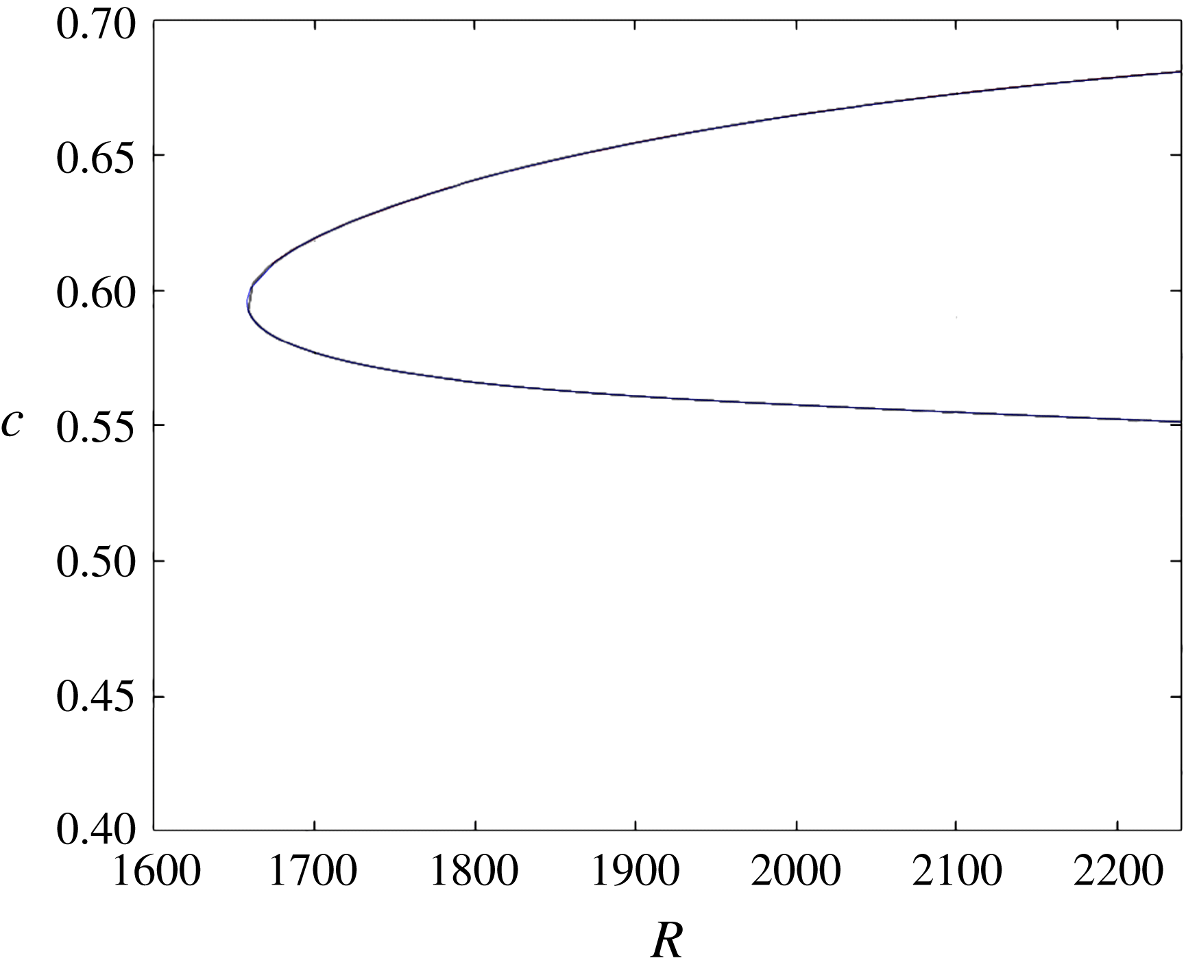
We reproduced the $S$ -symmetric solution of Wedin & Kerswell (Reference Wedin and Kerswell2004) for $k_{0}=2$ . The comparison of $c$ versus $R$ curve for ${\it\alpha}=1.55$ is shown in figure 1. Our calculations for $(N,M,P)=(45,8,5)$ (shown in blue) are indistinguishable from the grey curve of Wedin & Kerswell (Reference Wedin and Kerswell2004). The black curve, which sits on top of the blue curve, corresponds to higher resolution $(N,M,P)=(85,12,5)$ . More on comparisons with Wedin & Kerswell (Reference Wedin and Kerswell2004) appear in Ozcakir (Reference Ozcakir2014).

Figure 1.

$c$ versus $R$ for WK branch at ${\it\alpha}=1.55$ : grey curve: Wedin & Kerswell (Reference Wedin and Kerswell2004) calculations, blue curve: our $(N,M,P)=(45,8,5)$ calculations, black curve $(N,M,P)=(85,12,5)$ .

Figure 2.

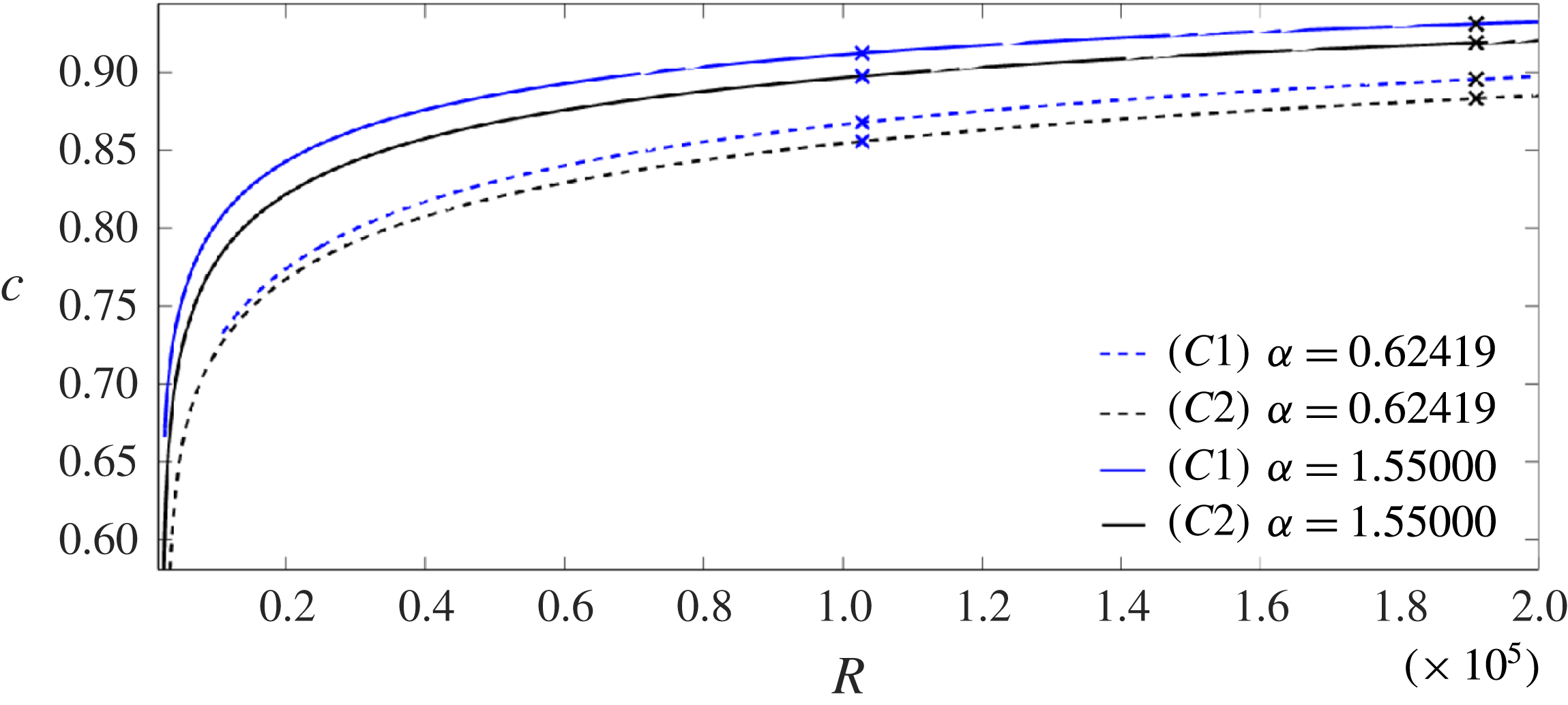
$c$ versus $R$ for different solution branches $C1$ , $C2$ for different axial wavelength ${\it\alpha}$ .

The scaling of rolls, streaks and waves for the computed WK solutions are roughly in agreement with the expected VWI scales for ${\it\delta}=1$ (see § 4.2), which is the same as the Hall & Sherwin (Reference Hall and Sherwin2010) scaling in channel flows, though our inability to continue the WK solution past about $R=11\,000$ hampered a more precise comparison between numerical results and $R\rightarrow \infty$ scaling results.

In addition, two new branches of travelling wave solutions have been found, which we denote as $C1$ and $C2$ . Besides the $S$ -symmetry (shift-and-reflect) the $C2$ branch also has ${\it\Omega}_{2}$ -symmetry (shift-and-rotate) as defined in Pringle, Duguet & Kerswell (Reference Pringle, Duguet and Kerswell2009), though this additional symmetry was not imposed in the numerical code. As pointed out earlier, in the representation (2.13), this corresponds to non-zero contributions only for even $k+l$ . For $k_{0}=2$ , this results in rolls and streaks having 4-fold azimuthal symmetry.

However, unlike other states calculated before, these new branches appear to have a collapsing vortex–wave structure toward the centre of the pipe as $R\rightarrow \infty$ , which will be quantified. These states are also different from the helical centre modes of Smith & Bodonyi (Reference Smith and Bodonyi1982) (confirmed for finite $R$ by Deguchi & Walton Reference Deguchi and Walton2013) where the dependence in ${\it\theta}$ and $z$ are linked; these spiral modes are special to $k_{0}=1$ . In figure 2 the phase speed $c$ is shown as a function of $R$ for the two wavenumbers ${\it\alpha}$ for $C1$ and $C2$ solutions for the lower branch. For $C1$ and $C2$ , we were able to compute solutions indefinitely with increasing $R$ , though resolution checks were limited to $R<2\times 10^{5}$ . In order to understand the asymptotic scaling of the new centre modes $C1$ and $C2$ , in figure 3, $1-c$ is plotted against $R$ on a log–log scale for large $R$ for two different values of ${\it\alpha}$ , with slopes $m$ ranging from $-0.32$ to $-0.38$ . This does not change much with higher resolution calculations shown by cross marks. In all the figures, slopes are quoted to two significant figures. A linear least square fit using data in the range $5\times 10^{4}<R<2\times 10^{5}$ is shown in dotted lines. We also noted that the slope in the regime $10^{5}<R<2\times 10^{5}$ is about three percent larger than the quoted value, suggesting that the solution may not have reached an ultimate asymptotic scale. Also, we noted a consistent tendency for the $1-c$ versus $R$ curve to steepen slightly with increasing ${\it\alpha}$ . For instance, the linear fit based on limited calculations for ${\it\alpha}=2.51$ in a large $R$ regime for the $C1$ solution shows $(1-c)\sim R^{-0.39}$ . (The notation ‘ ${\sim}$ ’ here and in the rest of the paper is not in the usual asymptotic sense; instead it is to be interpreted as the scaling.)

Figure 3.

$1-c$ versus $R$ in a log–log scale for different ${\it\alpha}$ for $C1$ and $C2$ solutions. Dotted lines are linear approximations to each curve using larger $R$ .

Figure 4.

Roll and streak profiles at $R=3940$ for ${\it\alpha}=1.55$ . (a) $C1$ ; (b) $C2$ ; (c) WK.

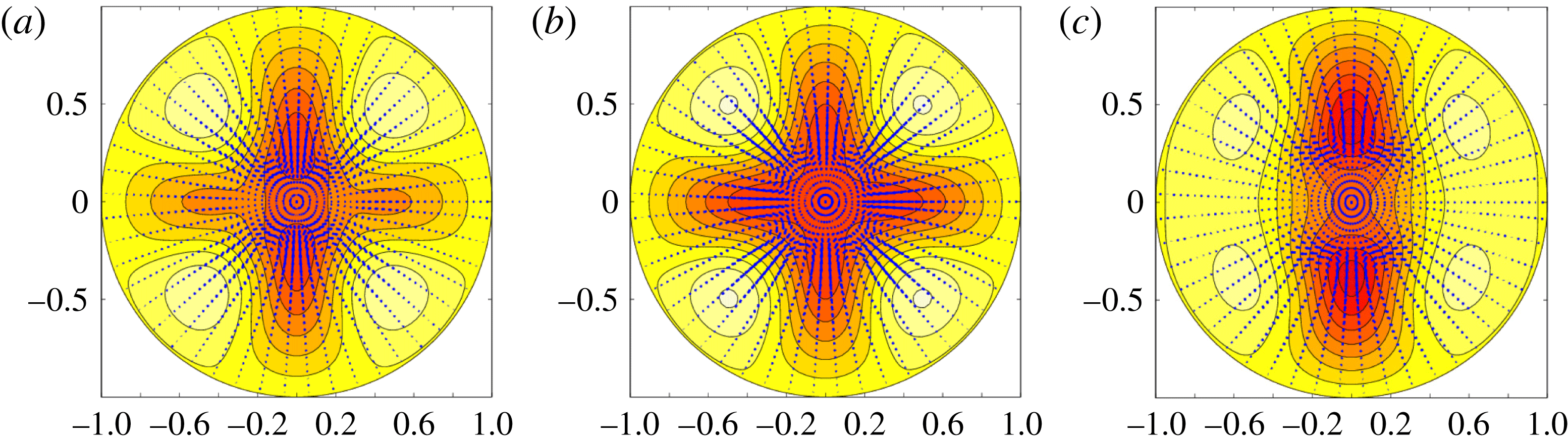
For these new states, the streamwise-averaged flows are displayed in a plane perpendicular to the pipe axis at several values of $R$ in figures 4–6 where the rolls $(U,V)$ are depicted using arrows whilst the streak velocity intensity is represented in colours, where the lighter colours correspond to positive values of streak $W$ , while darker colours correspond to negative $W$ . For comparison, we also present the WK solutions. (Note that Newton iteration failed to converge for the WK branch of solution for $R$ larger than about $11\,000$ , presumably because the solution approaches of a bifurcation point; this aspect was not pursued any further in this paper.) In all of the plots, the streak velocity ranges in the interval $[-0.4163,0.0963]$ . Note that the streaks get weaker as $R$ becomes larger, in accordance with asymptotic scaling results in § 4.

Figure 5.

Roll and streak profiles at $R=10^{4}$ for ${\it\alpha}=1.55$ . (a) $C1$ ; (b) $C2$ ; (c) WK.

Figure 6.

Roll and streak profiles at $R=10^{5}$ for ${\it\alpha}=1.55$ . (a) $C1$ ; (b) $C2$ .

The grey surfaces in figures 7 and 8 show surfaces of constant magnitude of streamwise velocity, excluding Poiseuille, at a value of 0.8 times the maximal value for two different $R$ values for the $C2$ state for specific ${\it\alpha}=1.55$ . We observed similar patterns for other values of ${\it\alpha}$ and for the $C1$ state. The coloured surfaces in the corresponding figures denote iso-surfaces of 0.8 times the maximal or minimal streamwise vorticity, with blue corresponding to positive vorticity and red corresponding to negative vorticity. Note that while the vortex structures become closer to the origin with larger $R$ , the streamwise velocity magnitude iso-surface, which is dominated by the streak component, does not shrink noticeably towards the origin. This feature is explained theoretically in § 4.4 and owes its origin to the mechanism found by Deguchi & Hall (Reference Deguchi and Hall2014a ).

Figure 7.

Streamwise velocity and vorticity iso-surfaces at 0.8 times extreme values at $R=50\,000$ for ${\it\alpha}=1.55$ for $C2$ .

Figure 8.

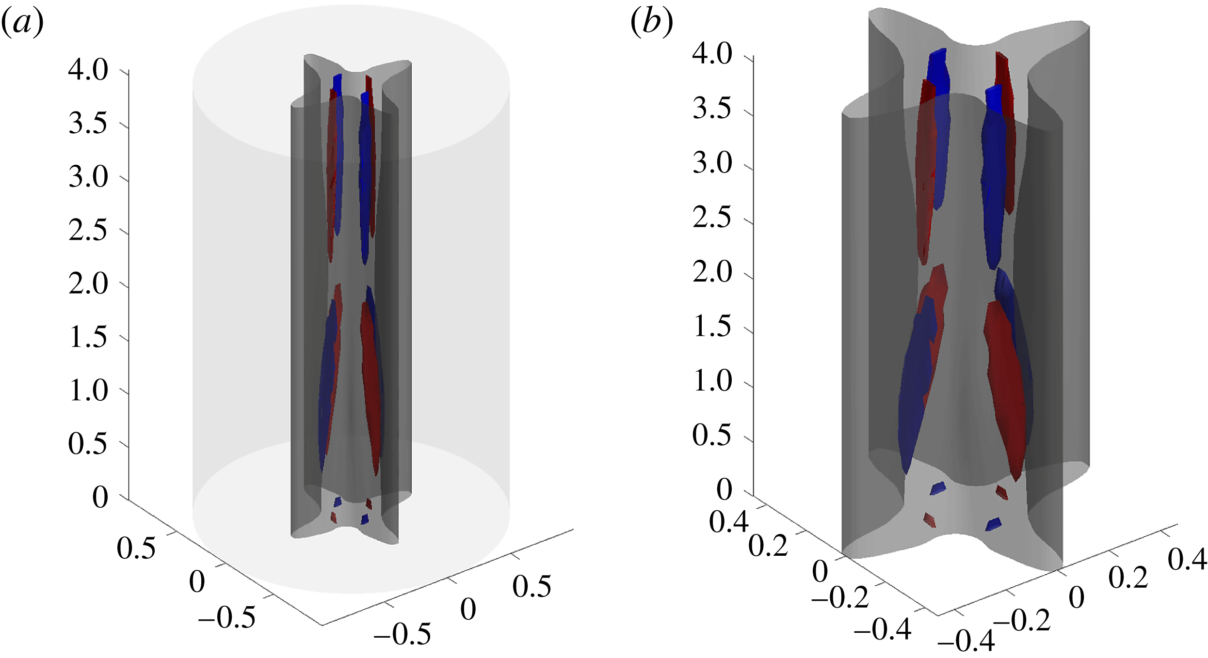
Streamwise velocity and vorticity iso-surfaces at 0.8 times extreme values at $R=191\,020$ for ${\it\alpha}=1.55$ for $C2$ .

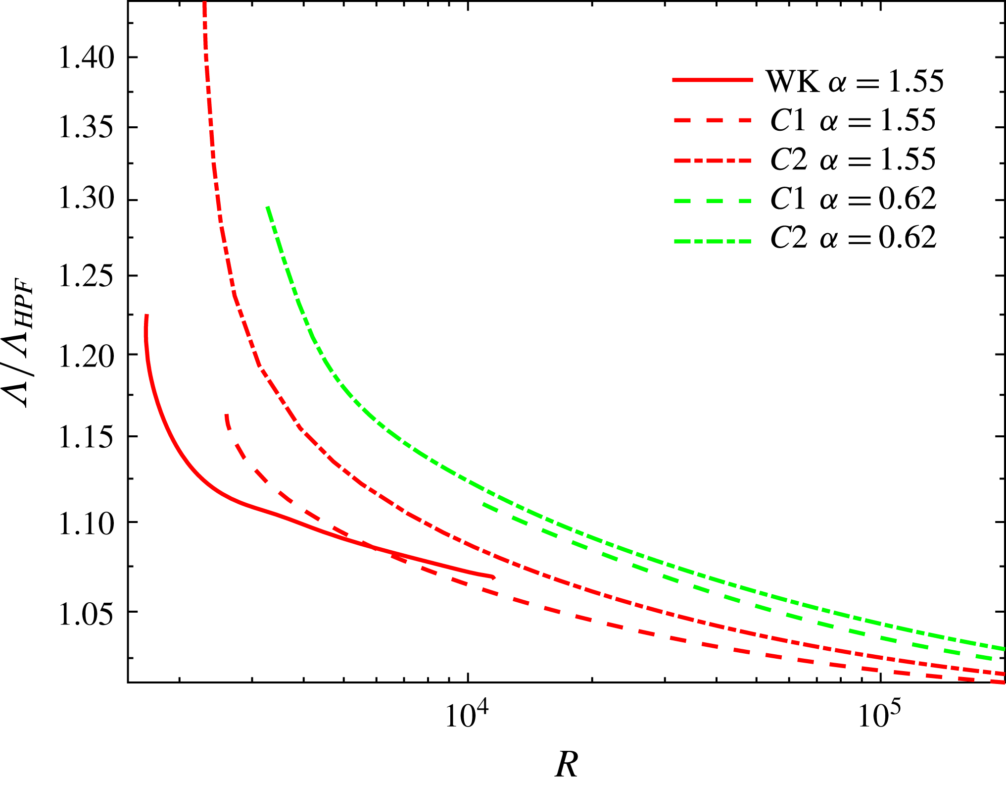
A quantity of general interest, which has some technological implications, is the friction factor ${\it\Lambda}$ associated with each of these states. ${\it\Lambda}$ is defined as

and $\overline{w}$ is the non-dimensional mean streamwise velocity given by

${\it\Lambda}$ is plotted against $R$ for WK, $C1$ , $C2$ solutions for three different values of ${\it\alpha}$ and compared against the Hagen–Poiseuille value of $64/R$ in figure 9.

Figure 9.

Friction factor ratio ${\it\Lambda}/{\it\Lambda}_{HPF}$ versus $R$ for lower branch WK, $C1$ and $C2$ solutions at ${\it\alpha}=1.55$ , ${\it\alpha}=0.624$ ; note ${\it\Lambda}={\it\Lambda}_{HPF}=64/R$ for Hagen–Poiseuille flow.

Now we report on other scaling features of the $C1$ , $C2$ solutions for large $R$ , restricted to $R<2\times 10^{5}$ . These include the behaviour of rolls, streaks and waves, including the location and magnitude of their maximum. We will also consider the collapsing of these solutions towards the centre of the pipe. It is convenient to define $k$ th azimuthal-amplitude functions for rolls, streaks and waves and their maximums as follows:

where the $l$ th axial Fourier component of wave velocity is defined for $l$ even and odd as:

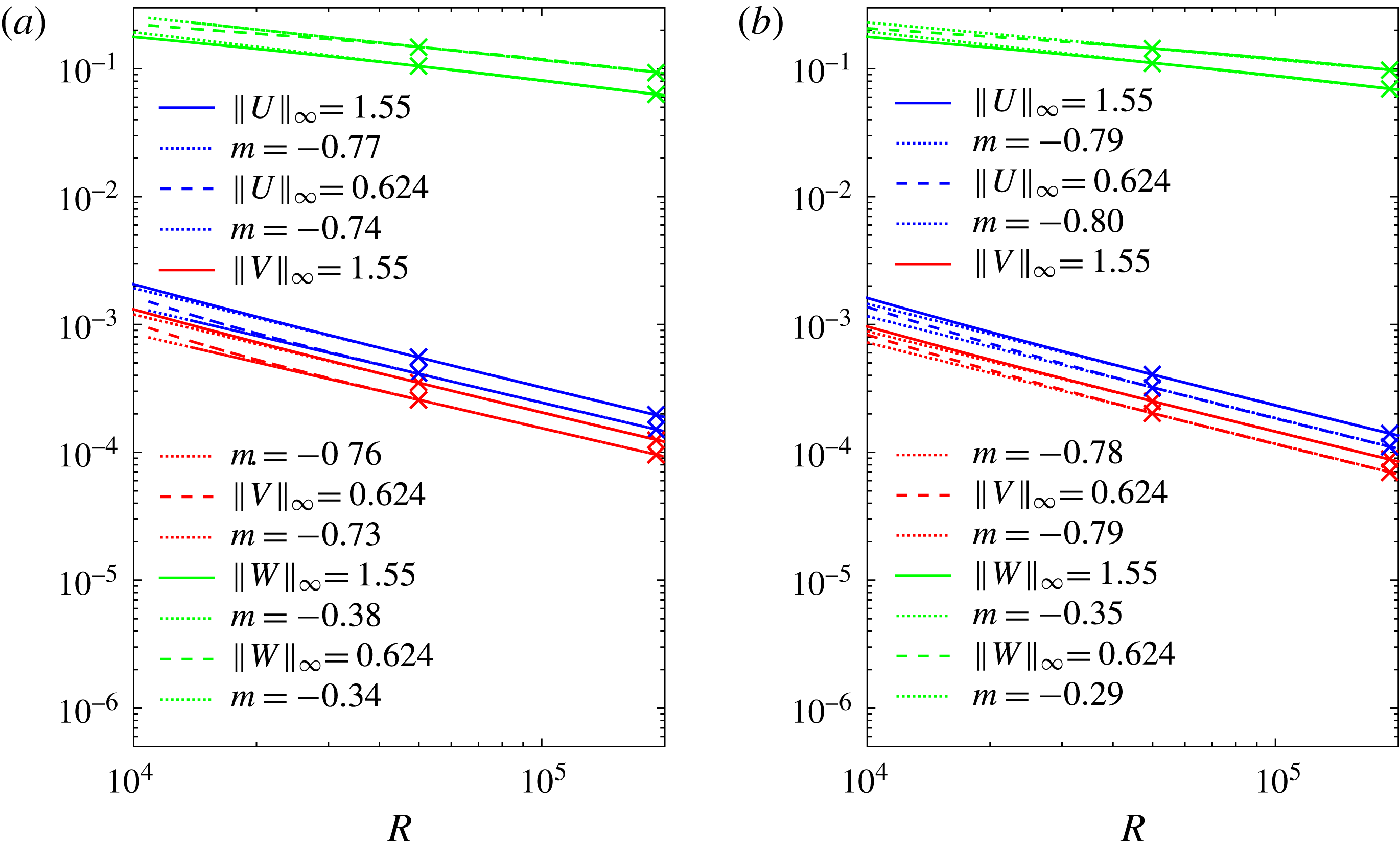
Figure 10 shows roll component sup-norms $\Vert U\Vert _{\infty }$ and $\Vert V\Vert _{\infty }$ and streak sup-norms $\Vert W\Vert _{\infty }$ for two different ${\it\alpha}$ as a function of $R$ on a log–log scale. The linear fittings on a log–log scale are based on a best-fit estimate of the data in the regime $5\times 10^{4}<R<2\times 10^{5}$ . The scaling for rolls for $C1$ ranges between $R^{-0.74}$ and $R^{-0.77}$ ; whilst the streak scaling ranges between $R^{-0.34}$ and $R^{-0.38}$ . We found a systematic trend for the slope to steepen slightly with increasing ${\it\alpha}$ . For instance, at ${\it\alpha}=2.51$ , the observed roll slope is close to $R^{-0.80}$ , while the streak slope is $R^{-0.40}$ . The roll scaling for $C2$ on the other hand ranges between $R^{-0.78}$ and $R^{-0.80}$ , whilst the streak size scaling ranges between $R^{-0.29}$ and $R^{-0.35}$ , again with slight dependence on ${\it\alpha}$ . At ${\it\alpha}=2.51$ , the observed roll slope is approximately $R^{-0.80}$ and the streak slope is $R^{-0.38}$ . The maximal streamwise wave amplitude for the $l$ mode, $\Vert A_{l}^{w}\Vert _{\infty }$ for $l=1,2,3$ is shown in figure 11(a,b) for two different values of ${\it\alpha}$ for both $C1$ and $C2$ . Note that the $l=1$ component for axial wave velocity scales somewhere between $R^{-0.50}$ and $R^{-0.52}$ for $C1$ , and $R^{-0.54}-R^{-0.55}$ for $C2$ , though the log–log scale also shows that the curves are yet to straighten completely for the larger $l$ range, and hence $R$ may not be large enough to reach the asymptotic regime for the larger $l$ cases. The mode dependence of the asymptotic trends is not unexpected since the effective Reynolds number is smaller for small scales, i.e. for larger $l$ or $k$ . For $l=2$ , the decay rate is approximately in the $R^{-0.51}-R^{-0.60}$ range. For $l=3$ the apparent scale is $R^{-0.5}$ for $C1$ at ${\it\alpha}=0.624$ , while it is $R^{-0.71}$ for $C2$ . Note that different $l$ modes have approximately the same decay rate in $R$ , suggesting that wave nonlinearity is important as $R\rightarrow \infty$ . In other words, the numerical results do not appear to be consistent with the VWI scenario of a dominating single wave mode.

Figure 10.

Supremum norm of roll components $(U,V)$ and of streak $W$ versus $R$ for (a) $C1$ and (b) $C2$ solution.

Figure 11.

Supremum over $(r,{\it\theta})$ of $A_{l}^{w}(r,{\it\theta})$ and $A_{l}^{\bot }(r,{\it\theta})$ at $l=1$ (blue lines), 2 (red lines), 3 (green lines) for (a,c) $C1$ and (b,d) $C2$ solutions for different ${\it\alpha}$ . Solid lines correspond to ${\it\alpha}=1.55$ , while dashed lines represent ${\it\alpha}=0.624$ . Dotted lines show linear fittings. Negative slopes of dotted lines (from top to bottom) are (a) $0.50,0.52,0.51,0.58,0.50,0.65$ , (b) $0.54,0.54,0.60,0.59,0.71,0.70$ , (c)  $0.76,0.76,0.86,0.80,0.84,0.83$ , (d) $0.78,0.78,0.88,0.88,0.69,0.78$ .

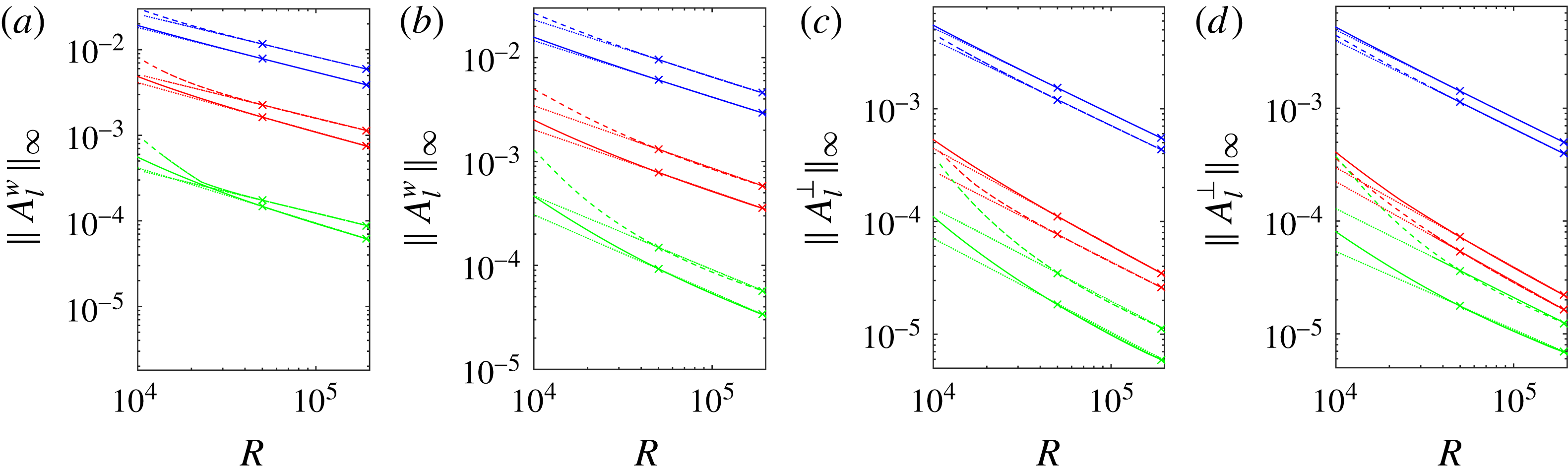
On the other hand, figure 11(c,d), show the scaling of the perpendicular wave amplitude $A_{l}^{\bot }(r,{\it\theta})$ for $C1$ and $C2$ . For $l=1$ , this scaling ranges between $R^{-0.76}$ and $R^{-0.78}$ for both $C1$ and $C2$ , while the $l=2$ mode corresponds to a faster decay rate in both cases; note $l=3$ curve is not as straight, suggesting it is further from reaching its asymptotic limit.

In figure 12, we plot $A_{k}^{U}(r)/A_{k,m}^{U}$ against $r/r_{m}$ for the $C1$ solution for two different values of ${\it\alpha}$ in (a,c,e) and (b,d,f). We notice that the curves have almost collapsed into a single graph, as might be expected if a single collapsing scale exists. The collapse is not as good for $k=3$ , apparently because the $R\rightarrow \infty$ asymptotic state has yet to be achieved for the smaller scales corresponding to larger $k$ . Note the decay of rolls in $r/r_{m}$ . This is explained asymptotically in § 4.3.

Figure 12.

Scaled radial roll-amplitude function $A_{k}^{U}(r)/A_{k,m}^{U}$ versus $r/r_{m}$ for $C1$ solution for $k=1,2,3$ for different $R$ . (a,c,e) ${\it\alpha}=1.55$ , (b,d,f) ${\it\alpha}=0.624$ .

Figure 13(a,b) shows $A_{k,m}^{U}$ against $R$ on a log–log scale for different values of $k$ for two different values of ${\it\alpha}$ . The corresponding radial location ( $r=r_{m}$ ), where the max $A_{k,m}^{U}$ is attained, is shown in figure 13(c,d) through a log–log linear fitting in the range $7\times 10^{4}<R<2\times 10^{5}$ .

Figure 13.

Maximal radial roll amplitude $A_{k,m}^{U}$ and its location $r_{m}$ for $k$ th azimuthal component versus $R$ for $C1$ solution for ${\it\alpha}=1.55$ (a,c) and ${\it\alpha}=0.624$ (b,d) when $k=1$ (cyan line), 2 (magenta line), 3 (green line). Dotted lines show linear fittings. Negative slopes of dotted lines (from top to bottom) are (a) $0.78,0.79,0.67$ , (b)  $0.84,0.65,0.66$ , (c) $0.23,0.21,0.22$ , (d) $0.23,0.22,0.22$ .

Figure 14.

Scaled radial roll-amplitude function $A_{k}^{U}(r)/A_{k,m}^{U}$ versus $r/r_{m}$ for $C2$ solution for $k=2,4,6$ for different $R$ . (a,c,e) ${\it\alpha}=1.55$ , (b,d,f) ${\it\alpha}=0.624$ .

We note that for the most dominant mode ( $k=2$ ), the scaling curves in (a,b) are close to straight lines in the range $5\times 10^{4}<R<2\times 10^{5}$ with the approximate behaviour $R^{-0.78}-R^{-0.84}$ , consistent with the decay rate of $\Vert U\Vert _{\infty }$ observed in figure 10. Beyond the most dominant mode, the graphs for other modes have not yet approached a straight line, suggesting that $R$ is not large enough to reach the asymptotic scaling regime for larger $k$ .

Notice in figure 13(c,d) that for the largest azimuthal component ( $k=2$ ), shown in magenta, $r_{m}$ scales approximately as $R^{-0.23}$ . This is nearly the same for other $k$ values ( $k=1,3$ ) though the curves become linear for larger $R$ .

Figures 14 and 15 give the same set of scaling results for the solution branch $C2$ . Note however that the odd values of $k$ are missing from the graph. This is because those components (within small calculation error) are zero since the corresponding solutions have the ${\it\Omega}_{2}$ -symmetry (shift-and-rotate) defined by Pringle et al. (Reference Pringle, Duguet and Kerswell2009).

Figure 15.

Maximal radial roll amplitude $A_{k,m}^{U}$ and its location $r_{m}$ for $k$ th azimuthal component versus $R$ for $C2$ solution for ${\it\alpha}=1.55$ (a,c) and ${\it\alpha}=0.624$ (b,d) when $k=2$ (cyan line), 4 (magenta line), 6 (green line). Dotted lines show linear fittings. Negative slopes of dotted lines (from top to bottom) are (a) 0.79, 0.71, 0.73, (b) 0.79, 0.74, 0.75, (c) 0.23, 0.23, 0.22, (d) 0.23, 0.23, 0.23.

Figure 16 shows streak amplitude $A_{k}^{S}(r)$ for different $R$ and $k$ with ${\it\alpha}=1.55$ and ${\it\alpha}=0.624$ for the $C1$ solution. It is to be noted that for $k=0$ , we have a very flat profile (see § 4.4 for a theoretical explanation). Because the roll effect on the streak is more global, $A_{k}^{S}(r)$ does not collapse in the same way for different $R$ as do rolls, though for $k\neq 0$ , there is a slight tendency of the maximum of the pattern to shift towards the origin for large $R$ .

Figure 16.

Profile of $C1$ -streak amplitude $A_{k}^{S}(r)$ versus $r$ for different $R$ and $k$ for given  ${\it\alpha}$ . (a,c,e,g) ${\it\alpha}=1.55$ , (b,d,f,h) ${\it\alpha}=0.624$ .

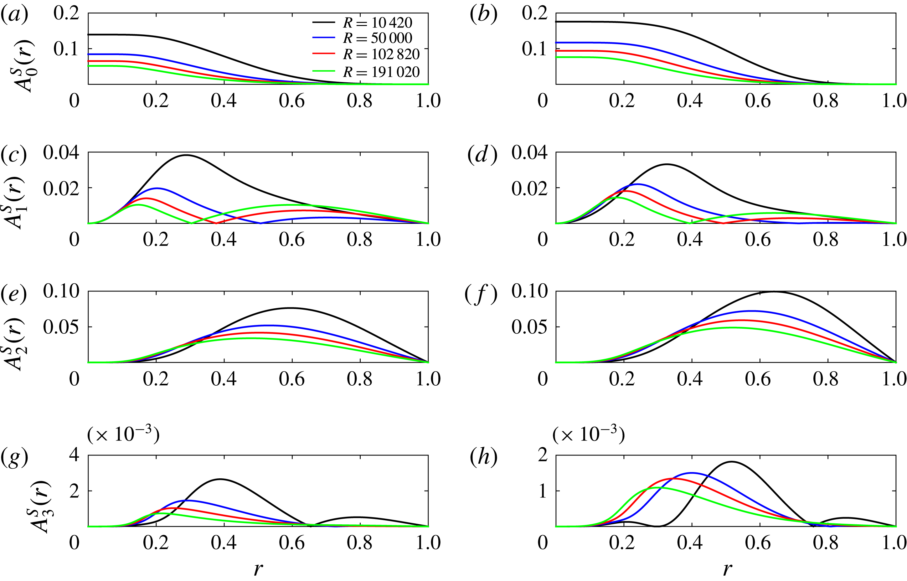
Figure 17(a,b) show the maximal streak amplitude $A_{k,m}^{S}$ against $R$ for different azimuthal wavenumber $k$ for $C1$ solution, while figure 17(c,d) show maximal radial location $r_{m}$ against $R$ . Note the $k=0$ curve is missing since $r_{m}$ is not well defined for a flat profile (see figure 16). The streak amplitude for the dominant $k=0$ mode scales as $R^{-0.37}-R^{-0.33}$ , close to the scaling of $\Vert W\Vert _{\infty }$ in figure 10.

Figure 17.

Maximal $k$ th streak amplitude $A_{k,m}^{S}$ versus $R$ and its location $r_{m}$ versus $R$ for $C1$ solution for $k=0$ (cyan line), 1 (magenta line), 2 (green line), 3 (red line) for ${\it\alpha}=1.55$ (a,c) and ${\it\alpha}=0.624$ (b,d). $k=0$ is missing in (c,d) since it has a flat profile. Dotted lines show linear fittings. Negative slopes of dotted lines (from top to bottom) are (a) 0.37, 0.33, 0.47, 0.53, (b) 0.33, 0.29, 0.33, 0.28, (c) 0.07, 0.23, 0.24, (d) 0.07, 0.21, 0.22.

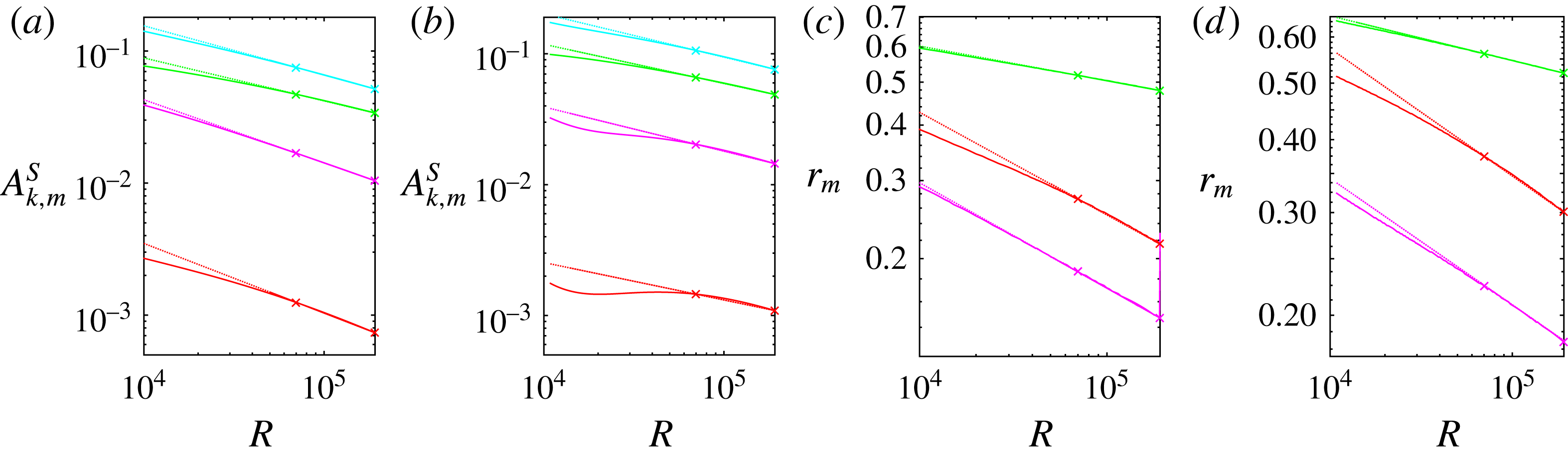
Figure 18 shows the streak-amplitude function $A_{k}^{S}(r)$ for different $R$ and $k$ for ${\it\alpha}=0.624$ and ${\it\alpha}=1.55$ for $C2$ solution. Again for $k=0$ , we observe a very flat profile.

Figure 18.

Profile of $C2$ streak amplitude $A_{k}^{S}(r)$ versus $r$ for different $R$ and $k$ for given  ${\it\alpha}$ . (a,c,e,g) ${\it\alpha}=1.55$ , (b,d,f,h) ${\it\alpha}=0.624$ .

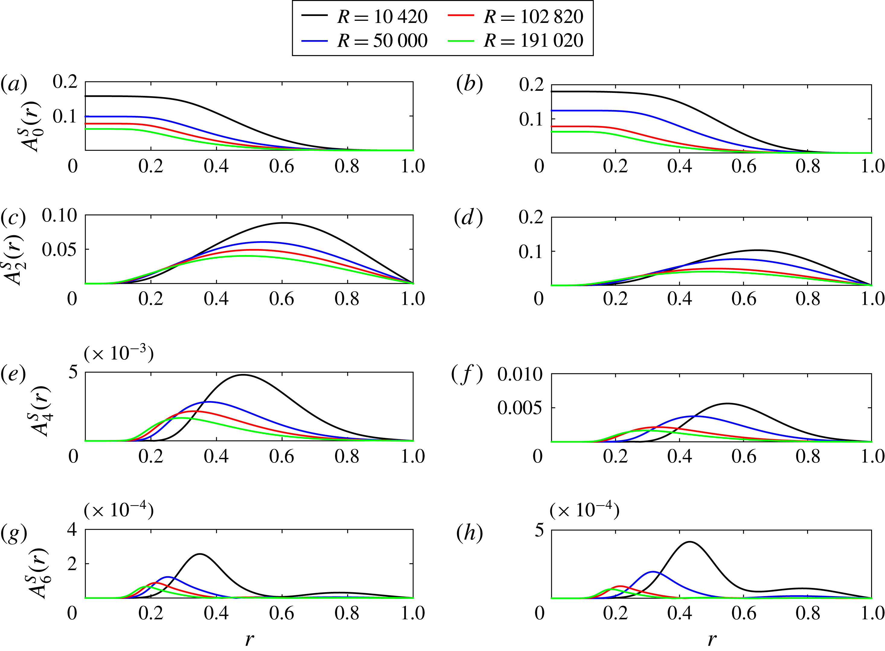
Figure 19(a,b) show the scaling of maximal streak amplitude $A_{k,m}^{S}$ with $R$ for different azimuthal wavenumber $k$ for the $C2$ solution, while figure 19(c,d) show the scaling of corresponding maximal location $r_{m}$ with $R$ . Once again the $k=0$ mode data is absent since $r_{m}$ is ill defined for a flat profile. The streak amplitude for the most dominant mode ( $k=0$ ) scales as $R^{-0.35}$ , $R^{-0.28}$ for ${\it\alpha}=1.55,0.624$ respectively, consistent with the scaling of $\Vert W\Vert _{\infty }$ in figure 10. Note that like the $C1$ solution, the maximal location $r_{m}$ is almost independent of $R$ ; this feature is explained theoretically in § 4.4.

Figure 19.

Maximal $k$ th streak amplitude $A_{k,m}^{S}$ versus $R$ and and its location $r_{m}$ versus $R$ for $C2$ solution for $k=0$ (cyan line), 2 (magenta line), 4 (green line), 6 (red line) for ${\it\alpha}=1.55$ (a,c) and ${\it\alpha}=0.624$ (b,d). $k=0$ is missing in (c,d) since it has a flat profile. Dotted lines show linear fittings. Negative slopes of dotted lines (from top to bottom) are (a) $0.35,0.31,0.40,0.45$ , (b) $0.28,0.26,0.33,0.45$ , (c) $0.07,0.19,0.23$ , (d) $0.07,0.17,0.22$ .

Figure 20.

Scaled axial wave amplitude $w_{kl}(r)/w_{k,l,m}$ versus $r/r_{m}$ for $C2$ solution at $l=1$ for different $k$ for ${\it\alpha}=1.55$ . (a) $(k,l)=(1,1)$ , (b) $(k,l)=(3,1)$ , (c) $(k,l)=(5,1)$ , (d)  $(k,l)=(7,1)$ .

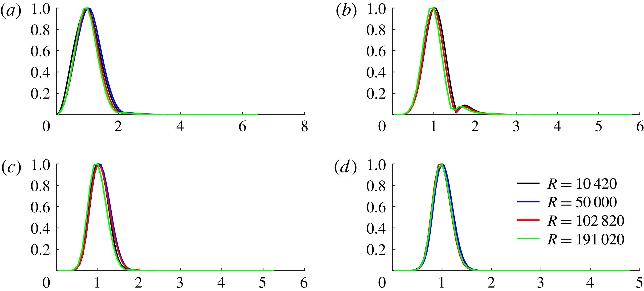
Figure 20 shows the collapse of the radial profile of the scaled axial wave amplitude $w_{k,l}(r)/w_{k,l,m}$ against $r/r_{m}$ (see (3.7c )) for $l=1$ for different $k$ and $R$ for $C2$ solution for ${\it\alpha}=1.55$ . A similar collapse was observed for the $C1$ solution and for other $l$ modes. For the radial wave components, the collapse was worse, presumably because of their smaller sizes and limitations in numerical accuracy. However, in all cases, we noted that the location of maximum $r_{m}$ shifted towards the origin for larger and larger Reynolds number at a rate similar to the collapse rate of rolls. Also note the rapid decay of the solutions with large $\hat{r}$ . This is shown to be a general property of all such states in § 4.5.

Figure 21.

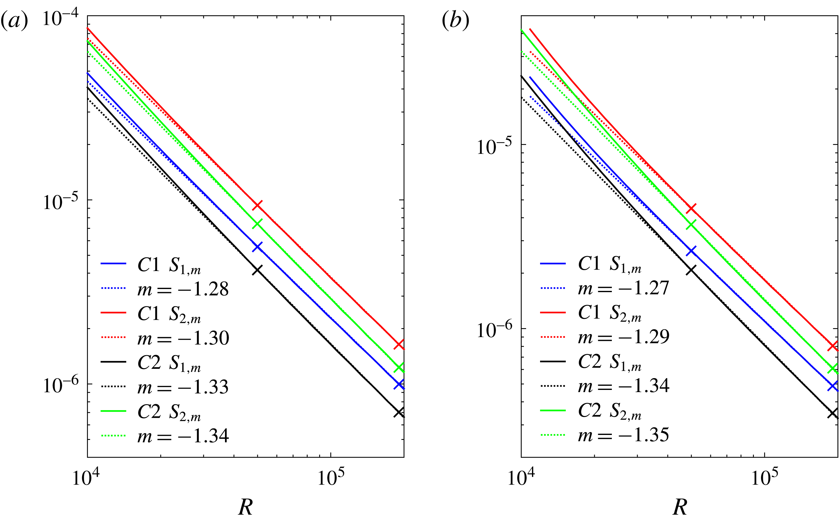
Scaling of maximal wave stresses $S_{1,m}$ , $S_{2,m}$ with $R$ for (a) ${\it\alpha}=1.55$ , (b)  ${\it\alpha}=0.624$ for both $C1$ and $C2$ solutions.

It is to be noted that the streak structure does not collapse with $R$ , at least not at the same rate as rolls and waves, and appears to extend to a region where $r/r_{m}$ is large. We explain this theoretically in § A.2. This is similar to the streak features observed in boundary-layer flows observed by Deguchi & Hall (Reference Deguchi and Hall2014a ).

To distinguish between a collapsing VWI state, where the wave amplitude is large in a critical layer only, and a nonlinear viscous core (NVC) state where axial wave and streak amplitude are of the same order throughout a shrinking core similar to the state discovered by Deguchi & Hall (Reference Deguchi and Hall2014a ) in a different context, we present the contour plots for Reynolds stresses. For a NVC state in a pipe (see § 4.1), we have a core shrinking as $R^{-1/4}$ , with $1-c=O(R^{-1/2})$ . The critical curve defined by $1-c-r^{2}+W(r,{\it\theta})=0$ has no significance in contrast to a VWI state. The Reynolds stresses $S_{1}$ and $S_{2}$ are defined as

and

We define $S_{j,m}:=\max _{(r,{\it\theta})}S_{j}(r,{\it\theta})$ and the corresponding maximal location $(r_{m},{\it\theta}_{m})$ in polar coordinates.

Figure 21 shows $S_{1,m}$ and $S_{2,m}$ against $R$ for ${\it\alpha}=1.55,0.624$ for the $C1$ and $C2$ solutions. It is clear that $S_{2,m}>S_{1,m}$ . Note for the $C1$ solution, $S_{1,m}$ , $S_{2,m}$ scale approximately as $R^{-1.27}$ , $R^{-1.29}$ respectively, while they scale as $R^{-1.34}-R^{-1.35}$ for the $C2$ solution. For stress plots, linear fittings involved the range $5\times 10^{4}<R<2\times 10^{5}$ . 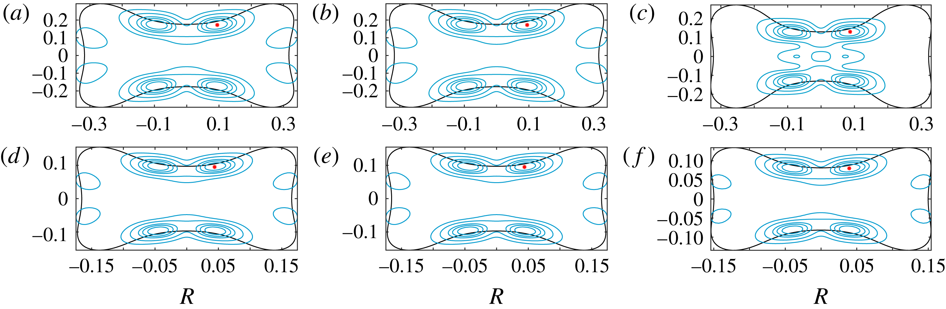The red points in figure 22 identify the locations of $(r_{m},{\it\theta}_{m})$ where $S_{2}$ attains a maximum for the $C1$ solution. Contour plots of $S_{2}(r,{\it\theta})$ where $S_{2}/S_{2,m}=0.9,0.8,0.7,0.5,0.3$ are also shown in the same figure for different $R$ and ${\it\alpha}$ . Though the contours for higher values of $S_{2}/S_{2,m}$ appear centred about the critical curve (where $1-c-r^{2}+W(r,{\it\theta})=0$ ) shown in black, they are far more spread out than expected for a critical curve (see Deguchi & Hall (Reference Deguchi and Hall2014b )). We observed similar features for the $C2$ solution.

Figure 22.

$S_{2}$ contours for $C1$ solution showing 0.9, 0.8, 0.7, 0.5 and $0.3\times S_{2,m}$ for three different values of $R$ for given ${\it\alpha}$ : ${\it\alpha}=0.624$ (a,d), 1.55 (b,e), 2.47 (c,f). Critical curve is shown in black, and location of $S_{2,m}$ shown in $\ast$ . (a–c) $Re=10\,420$ , (d–f) $Re=191\,020$ .

4 Large $R$ asymptotics for travelling waves

We discuss possible large $R$ asymptotic structure of travelling waves in a pipe when the axial wavenumber ${\it\alpha}$ is independent of $R$ . Assume we have a structure at the centre of the pipe of width ${\it\delta}\leqslant 1$ . Note ${\it\delta}=1$ corresponds to a non-collapsing structure characterized by $(1-c)^{-1}=O(1)$ . We introduce the rescaled radial variable $\hat{r}$ so that

Then, on subtracting Poiseiulle flow $(1-r^{2})\hat{\boldsymbol{z}}$ , and decomposing the remaining velocity into its axial component and its complement

it may be checked from the Navier–Stokes equation that $\boldsymbol{v}$ satisfies

We now introduce scaled variables

where $\boldsymbol{U}$ is the scaled roll and $\boldsymbol{u}$ the scaled wave components. The decomposition is made unique by requiring the axial wavelength average $\langle \boldsymbol{u}\rangle =0$ . Similarly, we decompose the axial velocity

where $W$ is the scaled streak and $w$ is the scaled axial wave velocity. We make the mild assumption that ${\it\delta}_{2}{\it\delta}^{-1}$ is of the same order of or smaller than ${\it\delta}_{3}$ , which without loss of generality implies

(Note replacing any ${\it\delta}$ by $2{\it\delta}$ or similar multiple of ${\it\delta}$ has no effect on the argument since this is equivalent to replacing the variable multiplying ${\it\delta}$ by a constant multiple, which does not affect the argument about the existence of the solution.) As will be seen later, ${\it\delta}_{4}\leqslant {\it\delta}_{2}/{\it\delta}$ , and so condition (4.7) requires that the largest possible scale of the axial wave amplitude does not exceed the streak. We make no further a priori assumption regarding the scales. We decompose pressure as

and define $c_{1}=O_{s}(1)$ , i.e. strictly of order one, so that

The estimated negative exponents of ${\it\delta}_{c}$ , ${\it\delta}$ , ${\it\delta}_{1}{-}{\it\delta}_{4}$ in powers of $R$ are obtained from data in $R\in (5\times 10^{4},2\times 10^{5})$ for $C1$ , $C2$ states and are displayed in table 1.

Table 1.

Estimated ${\it\gamma}$ values in a $R^{-{\it\gamma}}$ scaling.

Now, we return to theoretical arguments. Axial averaging $\langle \cdot \rangle$ of (4.3) and (4.4), the projection in the orthogonal plane, results in

In order to enforce the divergence condition (4.11), $P$ must appear in the leading-order asymptotics in (4.10). (We could have instead balanced pressure and viscous terms by taking ${\it\delta}_{5}={\it\delta}_{1}{\it\delta}^{-1}R^{-1}$ , in which case ${\it\delta}_{1}=1/{\it\delta}$ is the distinguished scale that brings inertial terms to the same order as viscous terms. However, this is equivalent to (4.12) and (4.13).) This implies

For the solutions with collapsing structure for which ${\it\delta}\ll 1$ , we impose the property $\boldsymbol{U}\rightarrow 0$ as $\hat{r}\rightarrow \infty$ (in the inner radial scale). On the other hand, for ${\it\delta}=1$ , the solution satisfies the homogeneous boundary condition $\boldsymbol{U}=0$ at $r=1$ . In either case, the leading-order balance in (4.10) as $R\rightarrow \infty$ must involve the viscous term for the steady non-trivial solution. Thus,

Using (4.12) and (4.13), (4.10) reduces to

We are constrained to choose without any loss of generality

since otherwise $\boldsymbol{U}=O_{s}(1)$ is inconsistent with the homogeneous boundary conditions and asymptotically small forcing in (4.10) and (4.14) when $R\gg 1$ . We note that the equality in (4.15) will hold if there is no critical layer and the wave magnitude is of the same order whenever $\hat{r}=O(1)$ . If there is a critical layer of thickness $\hat{{\it\delta}}\ll 1$ in the $\hat{r}$ scale, since wave $(\boldsymbol{u},w)=O(\hat{{\it\delta}})$ outside the critical layer, then $\max \{{\it\delta}_{2}^{2}/{\it\delta}_{1}^{2},{\it\delta}_{4}{\it\delta}{\it\delta}_{2}/{\it\delta}_{1}^{2}\}\gg 1$ in (4.14). In the limit when $\hat{{\it\delta}}\rightarrow 0$ , the forcing reduces to a delta function at the critical curve; consistent with $\boldsymbol{U}=O_{s}(1)$ in (4.14) provided a constraint between $\hat{{\it\delta}},{\it\delta}_{2},{\it\delta}_{1}$ is satisfied, which will be discussed in § 4.2.

Consider now the axial component of $\boldsymbol{v}$ in (4.3). Using (4.5) and (4.6), we obtain by axial averaging $\langle \cdot \rangle$ and using (4.13), the following equation for streak:

Requiring solution $W=O_{s}(1)$ in (4.16) with homogeneous boundary conditions implies that either the roll or wave term enters into the equation at the leading order, i.e.

where the latter possibility will be ruled out in the ensuing discussions. Consider now the equation for the wave $(\boldsymbol{u},w)$ defined uniquely by the property $\langle (\boldsymbol{u},w)\rangle =0$ , where $\boldsymbol{u}$ is the projection in the perpendicular plane, with radial and azimuthal components $(u,v)$ . From the axial component of (4.3), using (4.5), (4.6), (4.13) and (4.16), we obtain

For the components of the wave perpendicular to the cylinder, (4.3), with (4.5), (4.6), (4.13) and (4.14) imply

together with the divergence condition (4.4), which now implies:

Without any loss of generality,

as otherwise (4.20) results in $w$ being independent of $z$ to leading order, which from $\langle w\rangle =0$ , implies $w=0$ , which is inconsistent. Also, note that with condition (4.21), (4.15) implies

The parameter $c_{1}$ in the system of (4.18)–(4.20) must appear in the leading-order equation since it acts as an eigenvalue for non-zero solution to a system of homogeneous equations for $(\boldsymbol{u},w)$ with homogenous boundary conditions. Furthermore, the pressure must come into the leading-order balance in (4.19) as otherwise one cannot satisfy (4.20). Next, the term ${\it\delta}^{2}\hat{r}^{2}+{\it\delta}_{3}W$ must appear in the leading-order balance as otherwise using

the resulting leading-order equations $c_{1}\partial _{z}w=-{\it\delta}^{2}\partial _{z}\tilde{p}$ , $c_{1}\partial _{z}\boldsymbol{u}=-\boldsymbol{{\rm\nabla}}_{\bot }\tilde{p}$ (for some rescaled pressure $\tilde{p}$ ), together with (4.20) have no non-trivial solution. Thus, ${\it\delta}_{c}=O_{s}({\it\delta}_{3})$ since the possibility ${\it\delta}_{3}\ll {\it\delta}^{2}$ is ruled out in (4.17a,b ). Therefore, without any loss of generality, we have

Other terms appearing in each of (4.18) and (4.19) have to be of the same or of lower order than this term. For the pressure term to appear at the leading order in (4.19), as it must,

Further, all the other terms appearing in each of (4.18) and (4.19) cannot be any larger than ${\it\delta}_{c}$ (or ${\it\delta}_{3}$ ), which on using (4.13), (4.21), (4.22) and (4.25) implies without any loss of generality

Note that the last inequality gives ${\it\delta}_{4}\geqslant {\it\delta}_{2}/{\it\delta}$ , which together with (4.21) implies

Using (4.22), (4.24) and (4.27) and (4.25), we may rewrite (4.18) and (4.20) as

There are now two distinct possibilities:

5 Comparison between numerical computation and asymptotics

First, for VWI states when ${\it\delta}=1$ , the $R^{-1}$ scale for rolls, $O(1)$ scale for streaks and a maximal wave amplitude of $O(R^{-5/6})$ occurring in a critical layer of width $R^{-1/3}$ are, as expected, the same as Hall & Sherwin (Reference Hall and Sherwin2010) theory for channels. Because $(1-c)^{-1}=O(1)$ , and the critical layer is not close to the pipe centre, the geometric difference between a pipe and channel does not make any difference to the scale prediction. Indeed, the reported scale for rolls and critical-layer thickness from direct numerical calculation by Viswanath (Reference Viswanath2009) for the $S$ antisymmetric state is consistent with this prediction. Since asymptotic theory predicts that the wave-amplitude scaling $R^{-5/6}$ only persists over a layer of thickness $R^{-1/3}$ , and drops down to $O(R^{-7/6})$ outside the layer, it is clear that the kinetic energy of the waves is dominated by the critical-layer contribution and scales as $R^{-2}$ . The square root of the kinetic energy for $l=1$ , which is the dominant contribution, reported in Viswanath (Reference Viswanath2009) is $R^{-0.97}$ , not far from asymptotic theory. As mentioned before, we were unable to achieve numerical convergence for WK solutions for values of $R$ much larger than approximately 11 000 and so the agreement with the asymptotic scaling results for VWI-states is only qualitative.

On the other hand, the numerically computed $C_{1}$ , $C_{2}$ solutions appear to suggest a shrinking structure near the centre of the pipe as $R$ increases. For such cases, we have identified two theoretical possibilities in the § 4 as $R\rightarrow \infty$ :

Case (i) corresponds to a nonlinear viscous core with radial scaling ${\it\delta}=R^{-1/4}$ , with axial component of both streak and waves scaling as ${\it\delta}_{3}={\it\delta}_{4}={\it\delta}^{2}=R^{-1/2}$ while perpendicular components of both rolls and wave-velocity scaling as ${\it\delta}_{1}={\it\delta}_{2}={\it\delta}^{3}=R^{-3/4}$ . In this case, the wave speed perturbation $1-c$ scales as ${\it\delta}_{c}={\it\delta}^{2}=R^{-1/2}$ . The canonical equations that arise have been presented in § 4.6.

Case (ii) corresponds to a shrinking VWI state where ${\it\delta}=R^{-1/6}$ , ${\it\delta}_{3}={\it\delta}_{c}={\it\delta}^{2}=R^{-1/3}$ , ${\it\delta}_{1}=R^{-5/6}$ , ${\it\delta}_{2}=R^{-5/6}{\it\delta}^{-1/3}=R^{-7/9}$ , ${\it\delta}_{4}=R^{-5/6}{\it\delta}^{-4/3}=R^{-11/18}$ .

We notice from table 1 that ${\it\delta}_{1}{\it\delta}\approx 1/R$ , and ${\it\delta}_{c}\approx {\it\delta}_{3}$ as expected from the theory in either case (i) or (ii) though for the smaller ${\it\alpha}$ value, $C2$ solution shows a marked departure. We also notice that ${\it\delta}_{4}\approx {\it\delta}_{2}/{\it\delta}$ as expected from theory. However, ${\it\delta}^{2}\approx R^{-0.46}$ is not as close to ${\it\delta}_{3}\approx R^{-0.36}$ as expected from $R\rightarrow \infty$ consistent scaling. Nonetheless, the observed wave stress $S_{1}$ , $S_{2}$ scaling in figure 21 is consistent with asymptotic scaling argument $R^{-5/3}{\it\delta}^{-5/3}$ . Since our numerical results on improved resolution did not change the scales significantly, our conclusion is that the $R\rightarrow \infty$ asymptotic has been attained for some, but not all quantities. This should not be too surprising since, for instance, the scaling of the radial roll component seen in figure 15 shows that in some instances the largest-amplitude azimuthal component has a steeper slope than the second largest. Clearly, if the same slopes persist, the one which does not decay as rapidly with $R$ will have to dominate eventually. In this connection, it is to be noted further that Deguchi & Walton (Reference Deguchi and Walton2013) numerical scaling results for spiralling centre modes in a pipe were in agreement with Smith & Bodonyi (Reference Smith and Bodonyi1982) asymptotics for $R\geqslant 10^{8}$ ; hence it is not unexpected that our finite $R$ scaling results for $R\leqslant 2\times 10^{5}$ should deviate from $R\rightarrow \infty$ asymptotics.

To the extent that the observed core scaling ${\it\delta}$ (see table 1) in the numerically calculated range of $R$ is much closer to the theoretical $R^{-1/4}$ scale for NVC states than the $R^{-1/6}$ predicted for shrinking VWI states, we believe that the $C1{-}C2$ solutions are finite $R$ realizations of the NVC states. There is of course significant discrepancy between the numerically computed and asymptotically predicted ${\it\delta}_{3}$ , ${\it\delta}_{c}$ , but we believe this is because the $R$ range of calculations is not sufficiently large. It is noteworthy that $1-c$ versus $R$ curve consistently drifts towards a steeper slope for larger ${\it\alpha}$ , suggesting that this is indeed the case since in the wave analysis, ${\it\alpha}R$ , appears as a single large parameter. In this context, it may be pointed out that the $(1-c)\sim R^{-1/3}$ asymptotic prediction of spiral states of Smith & Bodonyi (Reference Smith and Bodonyi1982) is not realized accurately in numerical observations until $R\geqslant 10^{8}$ . Also, the Reynolds stress contour curves in figure 22 show that they are significantly spread out from the critical curve, which is quite different from the typical clustering observed in the VWI solution (Deguchi & Hall Reference Deguchi and Hall2014b ).

6 Discussion and conclusion

In this paper, we report the numerical computation of travelling wave solutions with shift-and-reflect symmetry through a numerical continuation process involving small alternate wall suction and injection in the azimuthal direction. Through linear stability analysis of the base state in the presence of suction–injection at a critical Reynolds number, a neutrally stable mode was used to determine an initial guess in a Newton iteration procedure to determine the finite-amplitude travelling wave solution. Far from the Hopf-bifurcation point in the parameter space, solutions were continued until suction–injection was completely turned off. This allowed recovery of previous solutions of Wedin & Kerswell (Reference Wedin and Kerswell2004), which provided an additional check on the numerical code. Though restricted only to solutions with 2-fold azimuthal symmetry, the process of calculation also resulted in the discovery of two previously unrecognized solution branches, marked by a collapsing structure near the centre of the pipe. We present many features of these solutions, identified as $C1$ and $C2$ , including scaling of the lower branch with Reynolds number in the range $5\times 10^{4}<R<2\times 10^{5}$ . The $C2$ branch of solution possesses shift-and-rotate symmetry, besides the shift-and-reflect symmetry, resulting in streaks and rolls having 4-fold azimuthal symmetry.

We also presented general asymptotic arguments for $R\rightarrow \infty$ to identify all possible scalings as $R\rightarrow \infty$ . For asymptotic states where the axial wavenumber is independent of $R$ , we identify two possible classes of solution. The first is a nonlinear viscous core (NVC), with core radius ${\it\delta}=R^{-1/4}$ , where axial components of fluid velocity scale as $R^{-1/2}$ , while velocity components perpendicular to the pipe axis scale as $R^{-3/4}$ . In this case, the wave speed $c$ satisfies $(1-c)\sim c_{1}R^{-1/2}$ as $R\rightarrow \infty$ , where $c_{1}$ is some order one constant. In the shrinking core, the inner equation is a fully nonlinear eigenvalue problem with $c_{1}$ as the eigenvalue; the equation resembles a fully-nonlinear Navier–Stokes with $R=1$ . This nonlinear viscous-core state is similar in many respect to the ones discovered by Deguchi & Hall (Reference Deguchi and Hall2014a ) in a boundary-layer flow. While the wave and roll components are localized in the shrinking core with algebraic decay as one moves away from the core, the streak component, though small, is the same size inside and outside the core, until wall effects become important. Unlike the boundary-layer flows of Deguchi & Hall (Reference Deguchi and Hall2014a ), there is no exponential growth of streak magnitude; instead some azimuthal component remains constant. We present evidence to suggest that the computed $C1{-}C2$ solutions are actually a finite $R$ realization of the NVC states with 2-fold azimuthal symmetry.

A second possibility is a class of vortex wave (VWI) states, which have rather different asymptotic structures from NVC. We identify, two sub-classes of VWI states, with core width ${\it\delta}=1$ or ${\it\delta}=R^{-1/6}$ depending on whether or not the vortex wave-structure collapse towards the pipe centre. For a vortex wave (VWI) solution, small linear waves of amplitude $O(R^{-5/6}{\it\delta}^{-4/3})$ concentrated mostly in a critical layer of width ${\it\delta}\hat{{\it\delta}}={\it\delta}(R{\it\delta}^{4})^{-1/3}$ drive rolls of magnitude $O(R^{-1}{\it\delta}^{-1/3})$ which generate streaks of magnitude ${\it\delta}^{2}$ . In this case $(1-c)=O({\it\delta}^{2})$ . Outside the critical layer, where viscosity is important but nonlinear interactions are still small, the wave components become smaller by a factor of $\hat{{\it\delta}}=(R{\it\delta}^{4})^{-1/3}$ . When ${\it\delta}=1$ , the scalings of these vortex wave solutions match those of Hall & Sherwin (Reference Hall and Sherwin2010) in a channel flow, and comparison with the so-called $S$ -antisymmetric numerical solution of Viswanath (Reference Viswanath2009) suggests that his solution is a finite $R$ realization of VWI states. Qualitative comparison with data suggests that the same is likely true for the Wedin & Kerswell (Reference Wedin and Kerswell2004) solution, though a more quantitative comparison is hampered by our inability to continue the Wedin & Kerswell (Reference Wedin and Kerswell2004) solution beyond about $R=11\,000$ . In the case of a shrinking core ${\it\delta}\ll 1$ , the conclusion that ${\it\delta}=R^{-1/6}$ is the only possibility requires us to consider how neutral modes are perturbed by higher-order effects, and the viscous critical layer plays a paramount role in this consideration.

To the extent that both VWI and NVC states arise from asymptotically small perturbations of the basic Poiseuille flow, their relevance to transition in turbulence is already recognized. In this context, we note that the shrinking core states have waves and rolls scaling with larger magnitude than for ${\it\delta}=1$ , in that sense, it takes a larger perturbation from Poiseuille to reach these new states. On the other hand, these shrinking core states have less interaction with the pipe boundaries, and are therefore likely more robust to perturbations at the boundaries. The stability and control of these states, which are likely to have slow and low-dimensional unstable manifolds, are important matters for further research with both theoretical and practical implications.