


INTRODUCTION
The pervasiveness and persistence of vote buying in elections around the world seems uncontested in the literature (Diaz-Cayeros, Estevez, and Magaloni Reference Diaz-Cayeros, Estevez and Magaloni2012; Finan and Schechter Reference Finan and Schechter2012; Golden and Min Reference Golden and Min2013). However, the mechanisms underlying the effectiveness of vote buying are less clear. Two nonexcludable approaches shed some light on this issue: the clientelist model and the distributive politics model.
In the models of clientelism, the political parties have access to private information on individual voters’ preferences, which is used to target citizens and promise (or advance) rewards in exchange for votes (Stokes Reference Stokes2005; Nichter Reference Nichter2008; Zarazaga Reference Zarazaga2016).Footnote 1 Although there is abundant anecdotal evidence about these transactions, the source of the money to pay the rewards and the brokers’ incentives to distribute it are less apparent. On the other hand, the distributive politics literature focuses on the most electorally rewarding allocation of (local) public goods or fiscal benefits (Dixit and Londregan Reference Dixit and Londregan1995; Lindbeck and Weibull Reference Lindbeck and Weibull1987). The latter rely on the assumption that campaign promises are fulfilled, which is unlikely to hold, especially in developing countries (Keefer and Vlaicu Reference Keefer and Vlaicu2007).
The differences between these two approaches are not innocuous. While the clientelist model focuses on vote buying at the individual level (Whose vote is cheaper to buy?), distributive politics models rest on targeting groups of individuals, typically defined by geographic or ethnic boundaries. Moreover, the literature on distributive politics predominantly neglects the issue of turnout.
In this paper, I argue that there is another way in which parties engage in vote buying using the government’s budget. Although, with less information than the local broker, incumbent politicians can employ the state’s resources to generate transactions with individual voters, for instance through discretionary social programs and grants. Hence, I propose a model in which the incumbent offers individual transfers, either to persuade and/or mobilize voters, despite having incomplete information on voters’ preferences.Footnote 2
I use microfoundations that incorporate vote and turnout buying in a model of distributive politics, in a context in which only the incumbent engages in clientelist strategies.Footnote 3 Voters are forward looking, but in the model there are no potential ramifications of their individual actions. Thus, like in the distributive politics models, the budget allocation is the most strategic decision in this game. Also, although the exchange of votes for rewards takes place at the individual level, the budget is managed in a centralized manner by the incumbent, with incomplete information on the voters’ preferences. I find that, contrary to the findings in the distributive politics literature, the incumbent concentrates his spending in opposition strongholds to minimize wasting resources on individuals who would have voted for him anyway. Furthermore, I show that, within those opposition strongholds, the largest share of expenses is devoted to mobilizing “weak” supporters and persuading “weak” opposition voters. Loyalists (or strong supporters) and “strong” opposition voters do not benefit from vote and turnout buying as much.Footnote 4
Related Literature and Supporting Evidence
Among the models of clientelism, Gans-Morse, Mazzuca, and Nichter (Reference Gans-Morse, Mazzuca and Nichter2014) and Morgan and Várdy (Reference Morgan and Várdy2010) are the only ones, to my knowledge, to propose a model in which a party can simultaneously consider vote and turnout buying as I do. The former, closer to my paper, considers a model with an incumbent or party machine that knows the individual voters’ preferences. This assumption allows the authors to characterize the optimal transfer to each individual. They conclude that, in equilibrium, there is some degree of double persuasion, that is, mobilization and persuasion, among the nonvoters who favor the opposition party. Hence, their conclusion resonates with mine. However, in my model, individual voters’ preferences are not observed and—as a result—the incumbent can only target groups of voters (core, swing or opposition strongholds).
Among the models of distributive politics, the findings are structured in terms of two competing hypotheses: whether more resources should be devoted to “swing” groups that—if convinced by political promises or spending—would alter the outcome of the election (Dixit and Londregan Reference Dixit and Londregan1995; Lindbeck and Weibull Reference Lindbeck and Weibull1987) or, on the contrary, whether the resources should be primarily allocated to “core” groups of voters who are most responsive to the promises (or transfers) and are thus cheaper to convince (Dixit and Londregan Reference Dixit and Londregan1995; Cox and McCubbins Reference Cox and McCubbins1986). Instead, in my model, parties cannot make binding promises, hence, they will offer take-it-or-leave-it transfers upfront; that is, before citizens vote.
Interestingly, even though targeting opposition strongholds is a new theoretical finding, there is evidence that supports it. Two of the largest poverty relief programs in Latin America fit my model closely: Bolsa Familia in Brazil (Fried Reference Fried2012) and the Plan Jefes y Jefas de Hogar (Head of Households Plan) in Argentina. Implemented at the turn of the century, both programs had the individuals as direct beneficiaries and implied a monthly paycheck from the national government (indeed, the former is a traditional conditional cash transfer program). Even if these programmes could be considered “programmatic” (the beneficiaries are defined strictly according to a policy goal), when governments operate with constraints on their budgets, they can prioritize some groups according to their political convenience. Fried (Reference Fried2012) makes a neat use of the Brazilian data and concludes that Bolsa Familia was not biased by political interests. He writes that “. . . a standard deviation shift in support for the incumbent presidential candidate (Lula) leads to 1% decrease in coverage. Shifts in the other indicators of core strategies were associated with at most a 2.4% change in coverage—but in the opposite direction to that predicted by existing theories” (p. 1048). In other words, although he finds evidence that the incumbent targeted more heavily the opposition strongholds, he concludes that Bolsa Familia was not used politically—maybe because of the lack of a theoretical framework of vote buying that fits his findings.
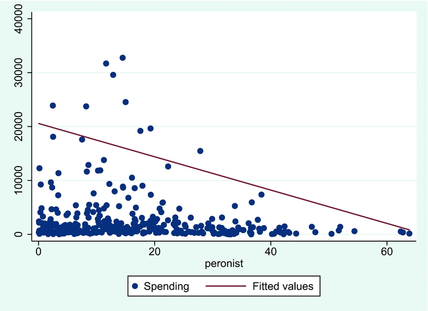
The case of Plan Jefes y Jefas de Hogar is similar. In 2002, the Peronist President, Eduardo Duhalde, set up this plan a few months before the presidential election. Figure 1 shows the number of beneficiaries by district, ordered from the average Peronist municipality to the most Peronist one. The red line shows the negative correlation between the incumbent’s spending and Peronist support in a municipality, from a linear estimation. Even though it cannot be interpreted as causal evidence and the context in Argentina after the crises was “critical” economically and politically, Figure 1 shows a pattern in which the opposition municipalities were targeted.
Districts with Relatively More Peronist-Leaning Preferences Receive Less Money

Although in a different setting, Curto-Grau, Herranz-Loncan, and Sole-Olle (Reference Curto-Grau, Herranz-Loncan and Sole-Olle2012) are also in line with my predictions: they study the construction of roads in Spain and they find that the “incumbent” builds more roads in opposition districts—that is, third-party districts—for political gain.Footnote 5
THE MODEL
In this economy, there are N d eligible voters per district d. Every citizen i in district d has a privately known ideology x i, drawn from the CDF F d(x) with bounded support  $[\underline{x}^d,\bar{x}^d]$ in X⊂ℜ, unimodal, and absolutely continuous. There are two national political parties, the incumbent I and the opposition O, with exogenous platforms X I and X O, in the policy space
 $[\underline{x},\bar{x}]=X\subset \Re$. F d(x) is common knowledge. Parties compete for office in a single-member election, in which the party with more votes across all districts is the winner. The incumbent party has a discretionary budget B from the federal funds that can be used to engage in “clientelist” competition by offering, before the election, a private take-it-or-leave-it transfer to individuals, tdi.
Citizens derive utility from their policy payoff, from their voting behavior, and from the transfers. We consider each of these in detail below. Consider first the utility derived from policy (the outcome contingent utility). Since we focus on large elections with a continuum of voters, the probability that a single vote is pivotal is zero for all voters and, hence, independently of the citizen’s action, he always gets an expected policy payoff, as it is commonly assumed in the literature (see for instance, Dekel, Jackson, and Wolinsky Reference Dekel, Jackson and Wolinsky2008). For simplicity, I do not write this expected policy payoff.
I now consider the utility derived from expressive voting (i.e., the act-contingent utility).Footnote 6 All citizens get a direct benefit b and bear a direct cost related to turning out to vote. The cost depends on the ideological distance to the party’s platform, quadratically. Hence, i’s expressive voting payoff is
 $$\begin{eqnarray*}
\nonumber \begin{array}{l@{\quad}l}b-(X_{P}-x_{i})^{2} &\text{if $i$ votes for party $P\in \lbrace I,O\rbrace $}\\
0&\text{if $i$ does not vote} \end{array}.
\end{eqnarray*}$$
Let us consider now the payoff from the transfers. The incumbent makes a take-it-or-leave-it offer of tdi dollars to each citizen i in district d, for whom the marginal valuation of a dollar is θ. If citizen i in district d accepts the transfer, the payoff of his electoral decisions would be constrained by the implicit vote-buying contract between the incumbent and the voter: if the citizen accepts tdi, he should show up to vote for the incumbent, otherwise he would suffer an expected punishment.Footnote 7 If the citizen rejects tdi, then he is excluded from the clientelistic exchange and he only gets the “expressive voting payoff.”
Let us now consider in detail the payoff of a voter who accepts tdi and therefore is subject to the vote-buying contract. If i accepts the transfer and votes for the incumbent, he gets an extra payoff of
 $$\begin{equation*}
\theta t_{i}^{d}.
\end{equation*}$$
There is evidence that indicates that voters do not believe that their vote is always secret (Gerber et al. Reference Gerber, Huber, Doherty, Dowling and Hill2013b illustrate it for the US) and they behave as if they could be punished if they deviate from a vote-buying “contract” (Gerber et al. Reference Gerber, Huber, Doherty and Dowling2013a; Vicente Reference Vicente2014; Finan and Schechter Reference Finan and Schechter2012). Hence, in line with the empirical evidence, let q d capture the perceived expected punishment (perceived monitoring probability of voting times the “punishment”). Then, if the voter accepts the transfer but votes for the opposition, he gets
 $$\begin{equation*}
\theta t_{i}^{d}-q^{d}.
\end{equation*}$$
Because the citizens have the option to reject a transfer and stay out of this clientelistic exchange—as it is well documented in Bratton (Reference Bratton2008) and references therein—the incumbent’s total expenditure in a district depends on the amount of citizens who accept the transfer, as will be clear in the constraint of the maximization problem in Equation (2).
Let  $\bar{q}$ capture the perceived monitoring probability of turnout times the punishment, with
 $q^d<\bar{q}$ for all d. Thus, the sum of all components leaves the citizen with the following utility:
 $$\begin{eqnarray}
\hskip90pt u^{d}_{i}=\left\lbrace \begin{array}{l@{\quad}l}0&\text{if $i$ does not vote}\\
b-(X_{P}-x_{i})^{2} &\text{if $i$ votes for party $P\in \lbrace I,O\rbrace $}\\
b-(X_{I}-x_{i})^{2}+\theta t_{i}^{d} &\text{if $i$ accepts the transfer and votes for I}\\
b-(X_{O}-x_{i})^{2}+\theta t_{i}^{d}-q^{d} &\text{if $i$ accepts the transfer and votes for O}\\
\theta t_{i}^{d}-\bar{q} &\text{if $i$ accepts the transfer and does not vote} \end{array}\right.. \qquad\quad\qquad
\end{eqnarray}$$
Districts are the artifact that allows the incumbent to target his resources. Districts differ in the technology available to monitor and punish voting behavior (q d), and in the underlying ideological bias drawn from F d(x). The incumbent allocates its budget B before the elections to buy votes and turnout through transfers, exploiting the observable differences across districts: the party directly observes q d, N d, and F d(x) and θ for each district.Footnote 8
Notice that all citizens in a given district look ex ante identical to the incumbent. Hence, I focus on the case in which he must offer the same transfer to all citizens in d, tdi = td, which depends on the budget B, the distribution of preferences {Fj}Dj = 1, and the monitoring technology {qj}Dj = 1.
The incumbent decides how to allocate the budget B across districts that differ in the cost of buying votes and/or turnout to affect the electoral outcome. Let SdI(td) and SdA(td) be the share of citizens that vote for the incumbent and the share of citizens that accept the transfer, in district d.Footnote 9 Then, in each district d, the incumbent distributes resources so that he maximizes the share of votes (V I):
 $$\begin{eqnarray}
\max _{t^{d}} V_{I}&=&\sum _{d}N^{d}\quad S_I^d(t^d) \text{\quad s.to\quad }\nonumber\\
B&\equiv& \sum _{d}B^{d}\ge \sum _{d} t^{d}N^{d}S_A^d(t^d).
\end{eqnarray}$$
The timing of the game is the following: At t = 0, all citizens observe the platforms X I and X O. At t = 1, the incumbent decides the level of individual transfers per district {td}d = Dd = 1. At t = 2, voters decide whether to accept the transfer or not. At t = 3, the election takes place, that is, citizens decide whether to vote, and for whom.
RESULTS
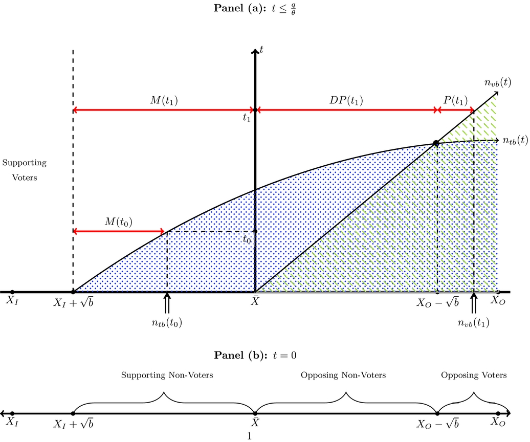
Following Gans-Morse, Mazzuca, and Nichter (Reference Gans-Morse, Mazzuca and Nichter2014), Figure 2(a) shows the ex ante classification of citizens: “supporting voters” or loyalists are those who would vote for the incumbent, with or without transfers, that is, with  $x_i\in [X_I-\sqrt{b},X_I+\sqrt{b}]$. Similarly, “opposing voters” would do the same with the opposition party, that is, with
 $x_i\in [X_O-\sqrt{b},X_O+\sqrt{b}]$. In between, there are the “supporting” and “opposing” nonvoters. Hence, vote buying (persuasion) takes place if an “opposing voter” votes for the incumbent due to the transfer (P(t) in Figure 2). Turnout buying (mobilization) takes place if a “supporting nonvoter” turns out to vote for the incumbent due to the transfer (M(t) in Figure 2). And, finally, vote and turnout buying (double persuasion) take place simultaneously if an “opposing nonvoter” turns out to vote for the incumbent (DP(t) in Figure 2).
Example of the Effect of a Transfer in a District

A Representative District
Let b, X I, and the policy space  $[\underline{x},\bar{x}]=X$ be such that
 $\underline{x}\ge X_{I}-\sqrt{b}$; therefore, according to Equation (1), in equilibrium there are no extremist voters who do not turn out, and mobilization can only occur among those voters located “between” the parties. This assumption simplifies the analysis without loss of generality.Footnote 10
Below, I define a vote-buying threshold n vb(t d) and a turnout-buying threshold n tb(t d). These thresholds identify the ideology of a voter who is indifferent between voting for the incumbent or not, and turning out or not, respectively.
Definition 1 For θt d < q d, let n tb(t d) and n vb(t d) be a turnout-buying threshold and a vote-buying threshold, respectively, such that
 $$\begin{equation*}
n_{vb}(t^{d})=\bar{X}+\frac{\theta t^{d}}{2\Delta _{X}},\quad \text{and}\quad n_{tb}(t^{d})=X_{I}+\sqrt{b+\theta t^{d}}.
\end{equation*}$$
Hence, Definition 1 implies a partition of the space (x i, t d), represented in Figure 2(b), for θt d < q d. The voters whose ideology is to the left of the minimum of n tb(t d) and n vb(t d) would accept the transfer and vote for the incumbent. But more importantly, the figure shows that all citizens whose ideology is to the right of the minimum threshold (in the shaded area) reject the transfer. These citizens are sufficiently far from X I to prefer rejecting the transfer than accepting it and voting for the incumbent, or the transfer is not large enough to “subsidize” them to show up to vote (even for the opposition).
The last point depends on the assumption θt d < q d, which ensures that any citizen who accepts the transfer shows up to vote for the incumbent, and so SdI(td) = SA d(td), which simplifies the maximization problem in Equation (2). Mechanically, this assumption rules out inefficiently large transfers that an optimizing incumbent would not do anyway. For θt d ≥ q d, some voters may accept the transfer but vote for the opposition. For instance, imagine the infinitesimal increase from a transfer  $t^d=\frac{q^d}{\theta }-\epsilon$ with ε → 0 to a transfer with ε = 0. This change implies a discontinuous increase in the incumbents’ expenses without any significant gain in votes, that is, all opposition voters accept the transfer but vote for the opposition anyway.Footnote 11
From the definition above, it can be checked that the turnout-buying threshold increases more rapidly with the transfers than the vote-buying one. Moreover, as we see in Figure 2(b), they are equal when they reach the “persuadable” voters, that is, when  $n_{tb}(t^{d})=n_{vb}(t^{d})=X_O-\sqrt{b}$. Hence, taking this information into account in the following proposition highlights the voters’ optimal response to transfers.
Proposition 1 For θt d < q d, there exists a turnout-buying threshold n tb(t d), and a vote-buying threshold n vb(t d), such that
1. If n tb(t d) ≤ n vb(t d) then all citizens with
 $x_{i}\in [ X_{I}+\sqrt{b},n_{tb}(t^{d})]$ are mobilized and those with x i ∈ [0, n tb(t d)) are also persuaded (i.e., double persuasion).
2. If n tb(t d) > n vb(t d) then,
(a) all voters with
$x_{i}\in [ X_{I}+\sqrt{b},X_{O}-\sqrt{b}]$ are mobilized and(b) all voters with x i ∈ [0, n vb(t d)] are persuaded.
(c) Thus, all voters with
$x_i\in [0,X_{O}-\sqrt{b})$ are doubly persuaded.


That is, the behavior of all the voters between the thresholds depends on the size of the transfer. If the transfer is large enough so n tb(t d) ≤ n vb(t d), then all the voters in between would have voted for the incumbent if they were voting, but they are not (because they are to the right of n tb(t d)). Hence, those voters are neither persuaded nor mobilized. When  $X_O-\sqrt{b}<n_{vb}(t^{d})<n_{tb}(t^{d})$, all voters between the threshold vote for the opposition, but the ones to the left of the vote-buying threshold vote for the incumbent: there are some who are mobilized to vote for the incumbent—2(a), there are some who are persuaded—2(b) and there are some who are both persuaded and mobilized—2(c). These three types of clientelism are represented in Figure 2(b) with the segments M(t 1), P(t 1), and DP(t 1), respectively. In the same figure, we see what would happen with a much smaller transfer, t 0, that only leads to mobilization, M(t 0).
Allocation across Districts
Notice that since there is no aggregate uncertainty and there are no incentives to save money, the incumbent allocates his resources to maximize his vote share, as in Dixit and Londregan (Reference Dixit and Londregan1996) and Cox and McCubbins (Reference Cox and McCubbins1986). Let n(t d) ≡ min{n vb(t d), n tb(t d)} for simplicity of notation. With θt d < q d, all citizens who accept the transfer vote for the incumbent, thus SdI(td) = SA d(td) equals
 $$\begin{eqnarray*}
&&F^{d}(\min \lbrace n_{vb}(t^{d}), n_{tb}(t^{d})\rbrace )-F^{d}(\underline{x})\nonumber\\
&&\quad =F^{d}(\min \lbrace n_{vb}(t^{d}), n_{tb}(t^{d})\rbrace )\equiv F^{d}(n(t^{d})).
\end{eqnarray*}$$
Since SdI = Fd(n(td)), the maximization problem in Equation (2) can be simplified to
 $$\begin{eqnarray}
\max _{t^d} V_{I}&=&\sum _{d}N^{d}F^{d}(n(t^{d}))\text{\quad s.to\quad}\nonumber\\
B&=&\sum _{d} t^{d}N^{d}F^{d}(n(t^{d})).
\end{eqnarray}$$
Let Δx ≡ X O − X I > 0, and let B be large enough such that there is some level of persuasion in each district. Then, I obtain an implicit solution for t d:Footnote 12
 $$\begin{eqnarray}
t^{d}=\frac{\sum _{d}t^{d}m^{d}+B}{\sum _{d}m^{d}}&-&\frac{2\Delta _{x}}{\theta }\frac{F^{d}(n(t^{d}))}{f^{d}(n(t^{d}))}\nonumber\\
&&\text{with }f^{d}(n(t^{d}))\equiv \frac{\partial F^{d}(n(t^{d}))}{\partial n(t^{d})}\nonumber\\
&&\text{and }m^{d}\equiv t^{d}N^{d}f^{d}.
\end{eqnarray}$$
In equilibrium, ∑t dm d and ∑m d are constants. Hence, from Equation (4), we see that the only thing that drives the differences between districts is the ideological distribution,  $\frac{F^{d}}{f^{d}}$, which we call the inverse of the “success voting ratio” (also known as the inverse of the “reversed hazard rate”).
The following proposition establishes the conditions for focusing on opposition strongholds, highlighting the importance of enlarging the, so far dichotomous, debate between core and swing districts.
Proposition 2 Let d ∈ {j, h} be such that h is the opposition stronghold relative to j, that is, with E(x i|i ∈ j) < E(x i|i ∈ h). Let their respective CDFs have bounded support in X. Hence  $t^h-t^j=\frac{2\Delta _x}{\theta }[\frac{F^{j}(n(t^{j}))}{f^{j}(n(t^{j}))}-\frac{F^{h}(n(t^{h}))}{f^{h}(n(t^{h}))}]$ is positive if and only if
 $\frac{F^{j}(n(t^{j}))}{f^{j}(n(t^{j}))}>\frac{F^{h}(n(t^{h}))}{f^{h}(n(t^{h}))}$. If so, a greater transfer is allocated in the opposition stronghold (t j < t h).
Proposition 2 shows under which conditions it is optimal to focus on opposition strongholds: that is, when they also have a larger “success voting ratio” f d(n(t d))/F d(n(t d)). In words, that is the case when the additional voters obtained by increasing the transfer, f d(n(t d)), are large relative to the citizens who accept it, F d(n(t d)). An implication of the proposition is that it is always optimal to focus on opposition strongholds if F d(n(t d)) satisfies the monotone likelihood ratio property.Footnote 13
Alternatively, as an example, I provide a more immediate approach with the uniform distribution, largely adopted in the literature on voting (since Downs Reference Downs1957). Let the ideologies in a district d be distributed uniformly on the support  $[\underline{x}^{d},\bar{x}^{d}]$, with
 $\bar{x}^{d}-\underline{x}^{d}$ constant across districts. Hence, the larger
 $\underline{x}^{d}$ is, the more a district is an opposition stronghold. Thus, my proposition delivers the following:
 $$\begin{equation*}
\frac{F^{d}(n(t^{d}))}{f^{d}(n(t^{d}))}=n(t^{d})-\underline{x}^{d}\text{\quad then\quad }t^{h}-t^{j}=k(\underline{x}^{h}-\underline{x}^{j}).
\end{equation*}$$
Intuitively, to mobilize more supporting nonvoters, and/or double persuade (mobilize and persuade) opposition nonvoters, larger transfers have to be disbursed. Nonetheless, since all citizens are offered the same transfer, the marginal cost of increasing the transfer by a penny to mobilize an indifferent citizen is that penny times all the voters who accept the transfer (which includes all supporting voters and some nonvoters, that is, the loyalists and some weak supporters). In terms of Proposition 2, with the uniform distribution, f(t) is constant but F(t) increases with t. Hence, the incumbent prefers to focus on those districts with the smallest amount of people accepting the transfer; that is, those with the smaller F(t), and so the larger success voting ratio, f(t)/F(t).
By the same reasoning, increasing the transfer to persuade an opposition nonvoter (weak opposer) implies that all supporters also get a larger transfer. Therefore, to minimize those “wasted resources,” the incumbent gives more money in districts with fewer supporters (i.e., opposition strongholds). In other words, the marginal cost of buying an additional voter is the total number of accepted transfers times the increase in the transfer. Thus, in districts with a greater numbers of loyalists, the marginal cost of buying an additional vote is large.
CONCLUSION
Gans-Morse, Mazzuca, and Nichter (Reference Gans-Morse, Mazzuca and Nichter2014) show that if we know voters’ preferences, it may be optimal to mobilize and persuade voters who prefer the opposition party. Instead, I assume that voters’ preferences are not known and I extend this idea into the literature on distributive politics by showing that the dichotomous discussion between swing and core districts should acknowledge the possibility of a third hypothesis: in a single-member election, opposition strongholds are the optimal target for an incumbent who aims to persuade and/or mobilize citizens.
In contrast with the seminal papers of distributive politics, I do not model campaign promises but an incumbent who spends the state’s resources to maximize his vote share in the upcoming elections. Moreover, these resources are offered individually to citizens in the form of take-it-or-leave-it transfers. As a consequence, when deciding the allocation of these resources, the incumbent takes into account the amount of citizens accepting the transfers. In other words, the incumbent does not want to transfer resources where the citizens would support him anyway. While, in Dixit and Londregan (Reference Dixit and Londregan1996), the optimal transfer only depends (positively) on the number of individuals who can be swayed by the proposed transfer (i.e., the density f(t) at the threshold),Footnote 14 in my model the transfer also depends (negatively) on the amount of individuals who accept it (i.e., the cumulative distribution function F(t) at the threshold). Therefore, the incumbent focuses his spending on opposition strongholds instead of core and swing districts when there is a large number of loyalists who would accept the transfer even though they would have voted for the incumbent without any transfer.
APPENDIX
Proofs
Proposition 1
The intuition is as follows. Only consider party I for now and use the thresholds in Definition 1: any citizen i in district d whose ideology lies to the left of n tb(t d) votes. And if his ideology is to the left of n vb(t d), he votes for the incumbent. Hence, suppose that n tb(t d) ≥ n vb(t d), then all the voters whose ideology is between these thresholds, if any would vote for the opposition because the incumbent paid them enough to turn out but not enough to vote for I. On the other hand, if n tb(t d) ≤ n vb(t d), then those voters in between the threshold would vote for the incumbent if they were paid enough to turn out. Thus, the smaller threshold is the one that always binds.
Proof. Individual i with  $x_{i}\le \bar{X}$ prefers to accept the transfer and vote for I to not voting if
 $t^{d}<\frac{q^{d}}{\theta }$ and if:
 $$\begin{eqnarray}
u_{i}(I|t^{d})&\ge& u_{i}(no\ turnout|no\ transfer)\Leftrightarrow | x_{i}-X_{I}|\nonumber\\
&\le& \pm \sqrt{b+\theta t^{d}}.
\end{eqnarray}$$
Call  $n_{tb}(t^{d})\equiv X_{I}+\sqrt{b+\theta t^{d}}$, and notice that, if there is only one party P, then a voter is mobilized if his ideology is such that
 $$\begin{eqnarray}
x_{i}&\in [X_{P}+\sqrt{b},\min \lbrace X_{P}+\sqrt{b+\theta t^{d}},\bar{x}^{d}\rbrace ]
\end{eqnarray}$$
or
 $$\begin{eqnarray}
x_{i}&\in [\max \lbrace X_{P}-\sqrt{b+\theta t^{d}},\underline{x^{d}}\rbrace ,X_{P}-\sqrt{b}].
\end{eqnarray}$$
For all i, the citizen prefers to accept the transfer  $t^{d}<\frac{q^{d}}{\theta }$ and vote for I to voting for O without the transfer if
 $$\begin{eqnarray}
u_{i}(I|t^{d})\ge u_{i}(O|no\ \ \textit{transfer}) \Leftrightarrow x_{i}\le &\bar{X}+\frac{\theta t^{d}}{2\Delta _{X}}.
\end{eqnarray}$$
Define  $n_{vB}(t^{d})\equiv \bar{X}+\frac{\theta t^{d}}{2\Delta _{X}}$. I do not focus on the case of accepting the transfer and voting for O because that is ruled out in Definition 1. Hence, if n tb(t d) > n vB(t d), then
 $$\begin{eqnarray*}
x_{i}&\le& \bar{X}+\frac{\theta t^{d}}{2\Delta _{X}}\Rightarrow x_{i}\le X_{I}+\sqrt{b+\theta t^{d}} \Rightarrow \nonumber \\
u_{i}(I|t^{d})&\ge& u_{i}(O|no\ \ \textit{transfer}),\nonumber \\
u_{i}(I|t^{d})&\ge& u_{i}(no\ turnout|no\ \ \textit{transfer}),\nonumber \\
u_{i}(I|t^{d})&\ge& u_{i}(O|t^{d}).
\end{eqnarray*}$$
Then, for all i with x i ≤ n vb(t d) votes for I. On the other hand, if
 $$\begin{eqnarray*}
\bar{X}+\frac{\theta t^{d}}{2\Delta _{X}}&\le& x_{i}\le X_{I}+\sqrt{b+\theta t^{d}} \Rightarrow \nonumber \\
u_{i}(I|t^{d})&<& u_{i}(O|no\ \ \textit{transfer}),\nonumber \\
u_{i}(I|t^{d})&\ge& u_{i}(no\ turnout|no\ \ \textit{transfer}),\nonumber \\
u_{i}(I|t^{d})&\ge& u_{i}(O|t^{d}),
\end{eqnarray*}$$
then, all i with n vb(t d) ≤ x i ≤ n tb(t d) would vote for O, without accepting the transfer.
Furthermore, if n vb(t d) ≥ n tb(t d), then for x i ≤ n tb(t d), it is straightforward that i would vote for I. And for n tb(t d) ≤ x i ≤ n vb(t d), the following holds:
 $$\begin{eqnarray*}
X_{I}+\sqrt{b+\theta t^{d}}&\le& x_{i}\le \bar{X}+\frac{\theta t^{d}}{2\Delta _{X}} \Rightarrow \nonumber \\
u_{i}(I|t^{d})&\ge& u_{i}(O|no\ \ \textit{transfer}),\nonumber \\
u_{i}(I|t^{d})&<&u_{i}(no\ turnout|no\ \ \textit{transfer}),\nonumber \\
u_{i}(I|t^{d})&\ge& u_{i}(O|t^{d}).
\end{eqnarray*}$$
Thus, citizen i would not vote. Notice that so far along the proof I have dismissed the “bound” of  $X_{O}-\sqrt{b}$, because if n tb(t d) = n vB(t d), then
 $X_{O}-\sqrt{b}=n_{tb}(t^{d})=n_{vB}(t^{d})$. ■
Proof of Proposition 2
 $$\begin{equation*}
\max \sum _{d}N^{d}F^{d}(n(t^{d}))\quad s.to\quad B\ge \sum _{d}F^{d}(n(t^{d}))N^{d}t^{d}
\end{equation*}$$
From manipulating the FOC as in Dixit and Londregan (Reference Dixit and Londregan1995), I obtain the general solution  $t^d=\frac{B+\sum {t^d m^d}}{\sum m^d}-\frac{F^d(t^d)}{f^d(t^d) n^{\prime }(t^d)}$. Assume θt d < q d for all d; and that the budget B is large enough such that
 $n(t^{d})=n_{vb}(t^{d})=\bar{X}+\frac{\theta t^{d}}{2\Delta _{x}}$, then, from the FOC for t i, I obtain
 $$\begin{equation*}
\frac{\theta }{2\Delta _{x}}f^{i}(n(t^{i}))N^{i}=N^{i}\lambda [t^{i}f^{i}(n(t^{i}))\frac{\theta }{2\Delta _{x}}+F^{i}(n(t^{i}))].
\end{equation*}$$
And dividing this equation by
 $$\begin{equation*}
\frac{\theta }{2\Delta _{x}}f^{j}(n(t^{j}))=\lambda [t^{j}f^{j}(n(t^{j}))\frac{\theta }{2\Delta _{x}}+F^{j}(n(t^{j}))],
\end{equation*}$$
obtained from t j’s FOC, I get
 $$\begin{equation*}
\frac{f^{i}(n(t^{i}))}{f^{j}(n(t^{j}))}=\frac{t^{i}f^{i}(n(t^{i}))\frac{\theta }{2\Delta _{x}}+F^{i}(n(t^{i}))}{t^{j}f^{j}(n(t^{j}))\frac{\theta }{2\Delta _{x}}+F^{j}(n(t^{j}))},
\end{equation*}$$
which can be rewritten as
 $$\begin{equation*}
t^{j}-t^{i}=\frac{2\Delta _{x}}{\theta }\left[\frac{F^{i}(n(t^{i}))}{f^{i}(n(t^{i}))}-\frac{F^{j}(n(t^{j}))}{f^{j}(n(t^{j}))}\right].
\end{equation*}$$





Comments
No Comments have been published for this article.