1 Introduction
The flow of a homogeneous or stratified fluid over an obstacle has been heavily studied from many points of view. A widely used approach for shallow fluids is the application of hydraulic concepts when the flow can be classified in terms of the upstream Froude number
 $F=U/c$
, where
 $U$
is the uniform upstream flow and
 $c$
is a linear long wave speed. For a homogeneous fluid with an undisturbed depth
 $h$
,
 $c=\sqrt{gh}$
, where
 $g$
is acceleration due to gravity, and for their analogous definitions for a stratified fluid, see Grimshaw & Smyth (Reference Grimshaw and Smyth1986) and Baines (Reference Baines1995). The flow is then supercritical, subcritical or transcritical depending on whether
 $F>1$
,
 $F<1$
or
 $F\approx 1$
. In the supercritical case waves generated at the obstacle propagate downstream, and the flow at the obstacle location is a locally steady elevation. In the subcritical case, waves propagate upstream and downstream away from the obstacle, and the flow at the obstacle location is a locally steady depression, accompanied by a steady lee waves downstream of the obstacle. Both these cases can be well understood qualitatively using linearised theory.
However, linearised theory fails in the transcritical regime, and then nonlinear shallow water theory leads to the determination of a locally steady hydraulic flow over the obstacle, with an upstream elevation and a downstream depression, each terminated by upstream and downstream propagating shocks. In the presence of wave dispersion, these shocks are resolved by undular bores. In the weakly nonlinear long wave regime the forced Korteweg–de Vries (KdV) equation has been invoked to describe this flow; see Akylas (Reference Akylas1984), Cole (Reference Cole1985), Grimshaw & Smyth (Reference Grimshaw and Smyth1986), Lee, Yates & Wu (Reference Lee, Yates and Wu1989), Binder, Vanden-Broeck & Dias (Reference Binder, Vanden-Broeck and Dias2005), Binder, Dias & Vanden-Broeck (Reference Binder, Dias and Vanden-Broeck2006), Grimshaw, Zhang & Chow (Reference Grimshaw, Zhang and Chow2007) and the review by Grimshaw (Reference Grimshaw2010). For a homogeneous fluid, extension to finite amplitudes in the long wave regime have been made by El, Grimshaw & Smyth (Reference El, Grimshaw and Smyth2006), El, Grimshaw & Smyth (Reference El, Grimshaw and Smyth2008), El, Grimshaw & Smyth (Reference El, Grimshaw and Smyth2009) and the comprehensive review by El & Hoefer (Reference El and Hoefer2016).
Although transcritical shallow water flow is now quite well understood for a single localised obstacle, there have been comparatively very few studies of the analogous case when there are two widely separated localised obstacles; see the recent work by Kim & Choi (Reference Kim and Choi2018) and the references therein. Previously, this motivated us to examine this case in Grimshaw & Maleewong (Reference Grimshaw and Maleewong2015, Reference Grimshaw and Maleewong2016) using the nonlinear shallow water equations for a homogeneous fluid, and the forced KdV equation respectively. In this latter case we found that the flow development can be defined in three stages. In the first stage there is the well-known development of undular bores upstream and downstream of each obstacle, with no interference from the other obstacle. In the second stage there is an interaction between the undular bore moving downstream from the first obstacle and the undular bore moving upstream from the second obstacle. In the third stage at very large times, there is evolution of this interaction, when one of the obstacles controls criticality. For equal obstacle heights, either one of the obstacles can control flow criticality, being the first obstacle when the flow is slightly subcritical, and the second obstacle otherwise. For unequal obstacle heights the larger obstacle controls criticality.
In this paper that study is extended to flow over two widely separated holes, or to a combination of a hole and an obstacle. Importantly for stratified fluids, we note that the terminology obstacle or hole can be reversed and depends instead on the relative polarity of the forcing term and the solitary wave solutions in the absence of any forcing (see Grimshaw & Helfrich (Reference Grimshaw and Helfrich2018)); for instance flow of a stratified fluid with a near-surface pycnocline over a bottom obstacle is equivalent to the flow of a homogeneous fluid over a hole. As in Grimshaw & Maleewong (Reference Grimshaw and Maleewong2016), we use the forced KdV framework, with a combination of some analysis and numerical simulations. The forced KdV equation is described in § 2 and numerical solutions are presented in § 3. We conclude in § 4.
2 Forced Korteweg–de Vries equation
The forced Korteweg–de Vries (fKdV) equation has been derived for water waves by Akylas (Reference Akylas1984), Cole (Reference Cole1985) and Lee et al. (Reference Lee, Yates and Wu1989), and for internal waves by Grimshaw & Smyth (Reference Grimshaw and Smyth1986); see also the review by Grimshaw (Reference Grimshaw2010). It is technically valid in the transcritical regime when
 $F\approx 1$
, and for the case of water waves, in non-dimensional units based on a length scale
 $h$
and a time scale
 $(h/g)^{1/2}$
, it is given by
 $$\begin{eqnarray}\displaystyle -\unicode[STIX]{x1D701}_{t}-\unicode[STIX]{x1D6E5}\unicode[STIX]{x1D701}_{x}+\frac{3}{2}\unicode[STIX]{x1D701}\unicode[STIX]{x1D701}_{x}+\frac{1}{6}\unicode[STIX]{x1D701}_{xxx}+\frac{f_{x}}{2}=0,\quad \unicode[STIX]{x1D6E5}=F-1. & & \displaystyle\end{eqnarray}$$
Here
 $\unicode[STIX]{x1D701}$
is the free-surface displacement above the free surface. The initial condition is
 $$\begin{eqnarray}\displaystyle \unicode[STIX]{x1D701}=0,\quad \text{at}~t=0, & & \displaystyle\end{eqnarray}$$
which corresponds to turning on the forcing at
 $t=0$
. Equation (2.1) is based on the usual KdV balance where
 $\unicode[STIX]{x1D701}\sim \unicode[STIX]{x1D6FC}^{2}$
,
 $\unicode[STIX]{x2202}/\unicode[STIX]{x2202}x\sim \unicode[STIX]{x1D6FC}$
,
 $\unicode[STIX]{x2202}/\unicode[STIX]{x2202}t\sim \unicode[STIX]{x1D6FC}^{3}$
,
 $\unicode[STIX]{x1D6E5}\sim \unicode[STIX]{x1D6FC}^{2}$
and
 $f\sim \unicode[STIX]{x1D6FC}^{4}$
where
 $\unicode[STIX]{x1D6FC}\ll 1$
is the governing small parameter. Analogous forced KdV equations hold for internal waves and in other physical contexts; see the cited references. Here when
 $f(x)>0$
we call the positive forcing an obstacle, and when
 $f(x)<0$
we call the negative forcing a hole, based on the water wave case. But, as already noted, in general positive (negative) forcing arises when the forcing has the same (opposite) polarity to the free solitary waves in the KdV equation. For instance, as already noted, for a stratified fluid when the pycnocline is near the surface, negative forcing corresponds to flow over an obstacle; see Grimshaw & Helfrich (Reference Grimshaw and Helfrich2018).
For a single localised forcing, with a maximum magnitude at
 $x=0$
of
 $\unicode[STIX]{x1D716}_{m}>0({<}0)$
for an obstacle or hole respectively, with effectively compact support such as a Gaussian, the transcritical problem can be solved asymptotically; see Grimshaw & Smyth (Reference Grimshaw and Smyth1986), the review by Grimshaw (Reference Grimshaw2010) and the recent summary in Grimshaw & Maleewong (Reference Grimshaw and Maleewong2016). In this asymptotic procedure, at first the linear dispersive term
 $\unicode[STIX]{x1D701}_{xxx}$
is omitted, and the resulting forced Hopf equation can be exactly solved using characteristics,
 $$\begin{eqnarray}\displaystyle \frac{\text{d}x}{\text{d}t}=\unicode[STIX]{x1D6E5}-\frac{3\unicode[STIX]{x1D701}}{2},\quad \frac{\text{d}\unicode[STIX]{x1D701}}{\text{d}t}=\frac{f_{x}}{2}. & & \displaystyle\end{eqnarray}$$
With the initial condition (2.2), this can be readily integrated explicitly. When characteristics intersect, a shock forms and must satisfy the shock condition
 $$\begin{eqnarray}\displaystyle (S-\unicode[STIX]{x1D6E5})[\unicode[STIX]{x1D701}]+{\textstyle \frac{3}{4}}[\unicode[STIX]{x1D701}^{2}]=0, & & \displaystyle\end{eqnarray}$$
where
 $[\cdot ]$
is the jump across the shock and
 $S$
is the shock speed. In the case of an obstacle,
 $f(x)>0$
, in the transcritical regime these shocks form upstream and downstream, leaving a localised steady solution with an upstream elevation and a downstream depression over the obstacle. Each of these is resolved with an undular bore; see the cited references. This transcritical regime is defined by
 $$\begin{eqnarray}\displaystyle 2\unicode[STIX]{x1D6E5}^{2}<3|\unicode[STIX]{x1D716}_{m}|. & & \displaystyle\end{eqnarray}$$
In the present case we also need to consider a hole,
 $f(x)<0$
, when in the transcritical regime (2.5) shocks form over the hole, and the solution there remains transient. However, in the case of a hole no analogous steady solution is possible, although in numerical simulations, upstream and downstream undular bores are again found. Outside the transcritical regime (2.5) the flow is respectively subcritical or supercritical when
 $$\begin{eqnarray}\displaystyle \unicode[STIX]{x1D6E5}<-\unicode[STIX]{x1D6E5}_{c}\quad \text{or}~\unicode[STIX]{x1D6E5}>\unicode[STIX]{x1D6E5}_{c},\quad \unicode[STIX]{x1D6E5}_{c}=\left\{\frac{3|\unicode[STIX]{x1D716}_{m}|}{2}\right\}^{1/2}. & & \displaystyle\end{eqnarray}$$
Shocks may form upstream and downstream of the obstacle respectively, and again are resolved with an undular bore.
In Grimshaw & Maleewong (Reference Grimshaw and Maleewong2016) we used the forced KdV equation to examine the flow when there are two widely placed obstacles with maximum magnitudes
 $\unicode[STIX]{x1D716}_{1,2}$
, located at
 $x_{a}<x_{b}$
respectively. In this paper we extend that study to flow over two holes, or to combinations of an obstacle and a hole. As in Grimshaw & Maleewong (Reference Grimshaw and Maleewong2016), there are several regimes to consider depending on
 $\unicode[STIX]{x1D6E5}$
and
 $\unicode[STIX]{x1D716}_{1,2}$
. The main regime of interest is when the flow is transcritical for each forcing separately, that is
 $\unicode[STIX]{x1D6E5}^{2}<\text{min}[|\unicode[STIX]{x1D716}_{1}|,|\unicode[STIX]{x1D716}_{2}|]$
, and then the solution evolves in three stages. In the first stage, upstream and downstream undular bores form from each forcing location separately. In the second stage the upstream elevation undular bore from the second obstacle will meet the downstream depression undular bore from the first obstacle. These interact and possibly then also modulate the upstream elevation undular bore from the second forcing location and the downstream depression undular bore from the first forcing location. Our main purpose here is to determine the outcome of that interaction. The third stage is when the solution appears to settle outside each obstacle, but with, in general, continuing wave interactions between the two forcing locations.
3 Numerical simulations
The forcing
 $f(x)$
is composed of two localised obstacles, two holes, or a combination of an obstacle and a hole, given by
 $$\begin{eqnarray}\displaystyle f(x)=\unicode[STIX]{x1D716}_{1}\exp (-(x-x_{a})^{2}/w)+\unicode[STIX]{x1D716}_{2}\exp (-(x-x_{b})^{2}/w), & & \displaystyle\end{eqnarray}$$
where
 $\unicode[STIX]{x1D716}_{1}$
and
 $\unicode[STIX]{x1D716}_{2}$
are the magnitudes,
 $x_{a}$
and
 $x_{b}$
are the forcing locations and
 $w$
is the width, assumed to be the same for both forcing terms. The numerical scheme is described in appendix A.
3.1 Single hole
 $(\unicode[STIX]{x1D716}_{1}<0,\unicode[STIX]{x1D716}_{2}=0)$

At first we reconsider the case of a single hole; see Grimshaw et al. (Reference Grimshaw, Zhang and Chow2007) for a comprehensive account. We set the location of the single hole as
 $x_{a}=-2000$
.
 $\unicode[STIX]{x1D716}_{1}=\unicode[STIX]{x1D716}=-0.01$
with a negative value for a hole, while here
 $\unicode[STIX]{x1D716}_{2}=0$
. First we consider the case of very wide hole,
 $w=10\,000$
, in order to compare with the theoretical results for broad forcing described above in § 2, Note that here
 $\unicode[STIX]{x1D6E5}_{c}=0.12$
, see (2.6), so we expect the transcritical regime to be
 $0.88<F<1.12$
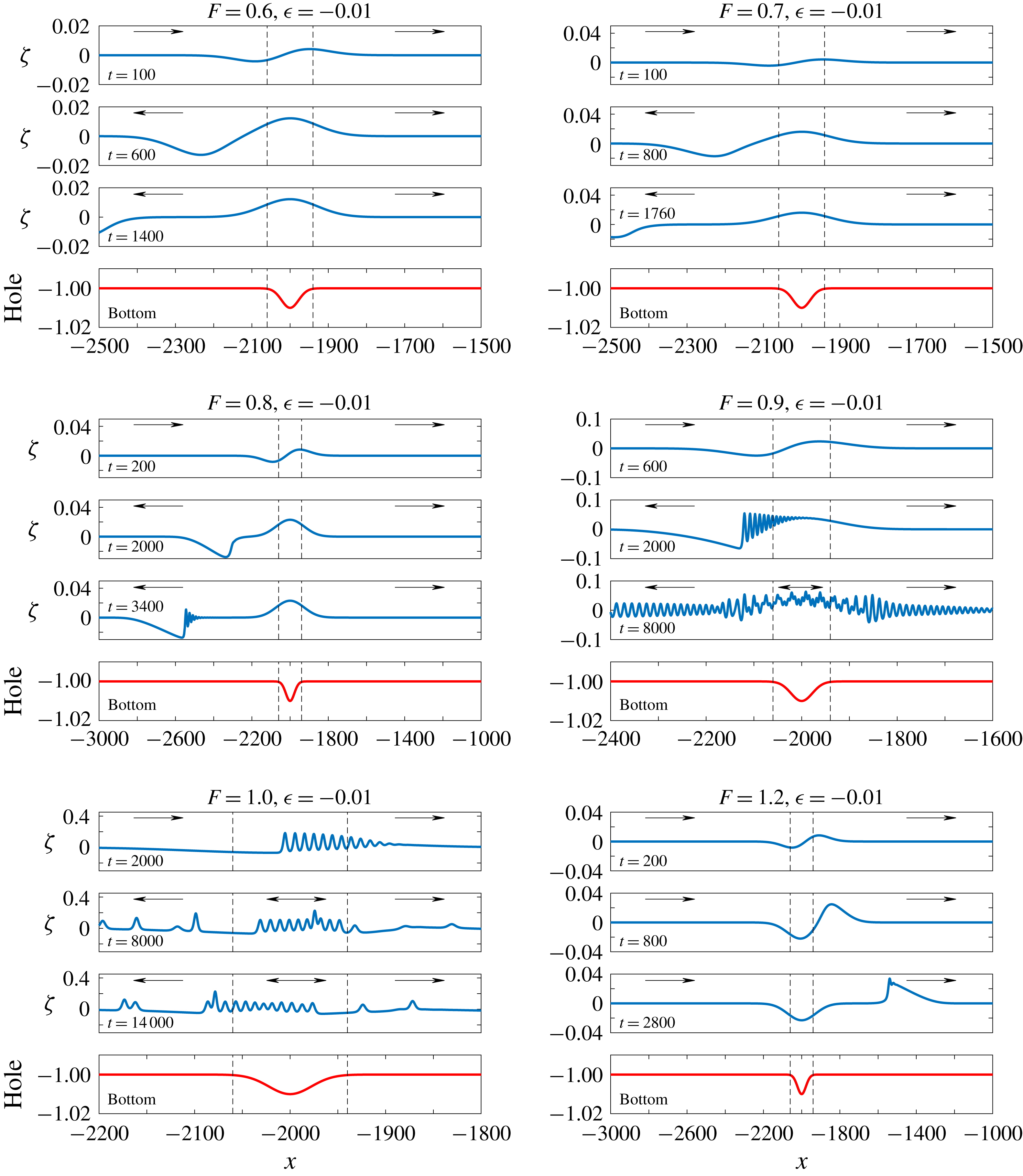
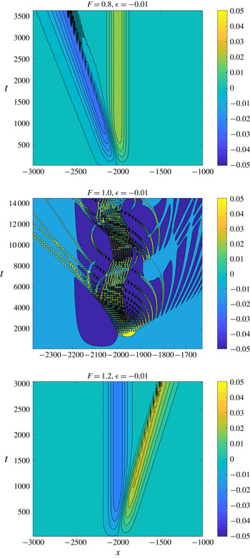
. The simulation results, ranging from subcritical to supercritical flows, are shown as
 $x{-}t$
plots in figure 1, and some corresponding contour plots in figure 2. The flows are subcritical when
 $F=0.6$
and
 $0.7$
with a steady elevation over the hole, while a rarefaction wave moves upstream; this rarefaction wave eventually steepens and forms a weak undular bore far upstream (not shown in these plots). The amplitude of the elevation wave over the hole increases as
 $F$
increases. In the case
 $F=0.8$
the flow over the hole is subcritical as expected, but the upstream rarefaction wave with the development of an undular bore are now visible. This indicates nonlinear behaviour even when the hole amplitude is small and the width is large. The flow is transcritical when
 $F=0.9$
and oscillating waves are trapped around and over the hole region. This oscillatory behaviour over the hole can be seen more clearly when
 $F=1$
. Groups of small-amplitude waves travel between the left border and the right border of the hole while some waves escape past these borders generating upstream and downstream transient waves. The flow becomes supercritical when
 $F=1.2$
with a steady depression wave over the hole while there is a transient solitary wave moving downstream.
Subcritical to supercritical flows over a very wide hole,
 $w=10\,000$
,
 $\unicode[STIX]{x1D716}=-0.01$
.

Contour plot for
 $F=0.8,1.0$
and
 $1.2$
when
 $\unicode[STIX]{x1D716}=-0.01$
and
 $w=10\,000$
.

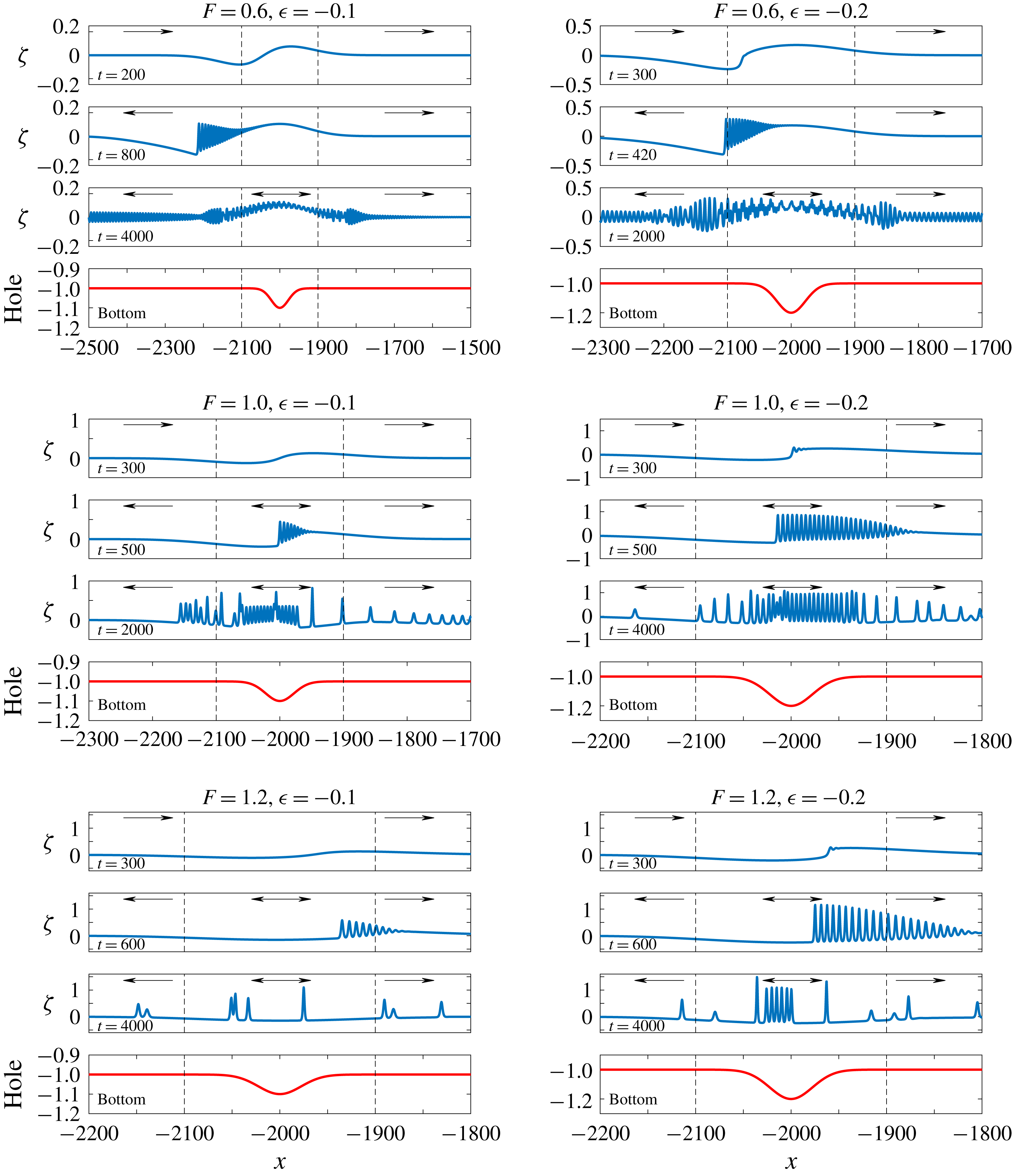
Next we increase the hole magnitude to
 $\unicode[STIX]{x1D716}=-0.1,-0.2$
and the results are shown in figure 3. Now
 $\unicode[STIX]{x1D6E5}_{c}=0.39,0.55$
respectively, so the we expect the flow to be transcritical for
 $0.61<F<1.39$
,
 $0.45<F<1.45$
respectively, and the simulations indicate that the flow is now effectively transcritical for all the cases shown, with transient waves over the hole. The waves that are generated at an early stage around the left border of the hole move back to the right border of the hole. Some waves can propagate downstream depending on the values of
 $F$
and the hole magnitude. We see that some transient waves are wrapped around the hole when
 $|\unicode[STIX]{x1D716}|$
is relatively large. Subcritical flow occurs at lower values of
 $F$
and supercritical flow occurs at higher values of
 $F$
as
 $\unicode[STIX]{x1D716}_{1}$
becomes larger. At an early stage for each case of
 $F$
when
 $\unicode[STIX]{x1D716}$
is fixed, the
 $x$
-location that produces moving-back waves connecting to an upstream rarefaction occurs inside the hole area. For example, when
 $F=1$
the
 $x$
-location may occur near the centre of hole, but the
 $x$
-location may occur near the left border of the hole when
 $F=0.8$
.
Subcritical to supercritical flow over a very wide hole,
 $w=10\,000$
,
 $\unicode[STIX]{x1D716}=-0.1$
and
 $-0.2$
.

3.2 Two holes
$(\unicode[STIX]{x1D716}_{1}<0,\unicode[STIX]{x1D716}_{2}<0)$

There are many parameters to consider and we have carried out many simulations. Only a representative sample are presented here, all with a fixed distance between the two forcing centres,
 $x_{a}=-100,x_{b}=100$
and fixed widths,
 $w=50$
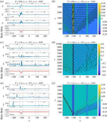
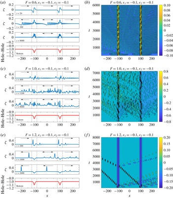
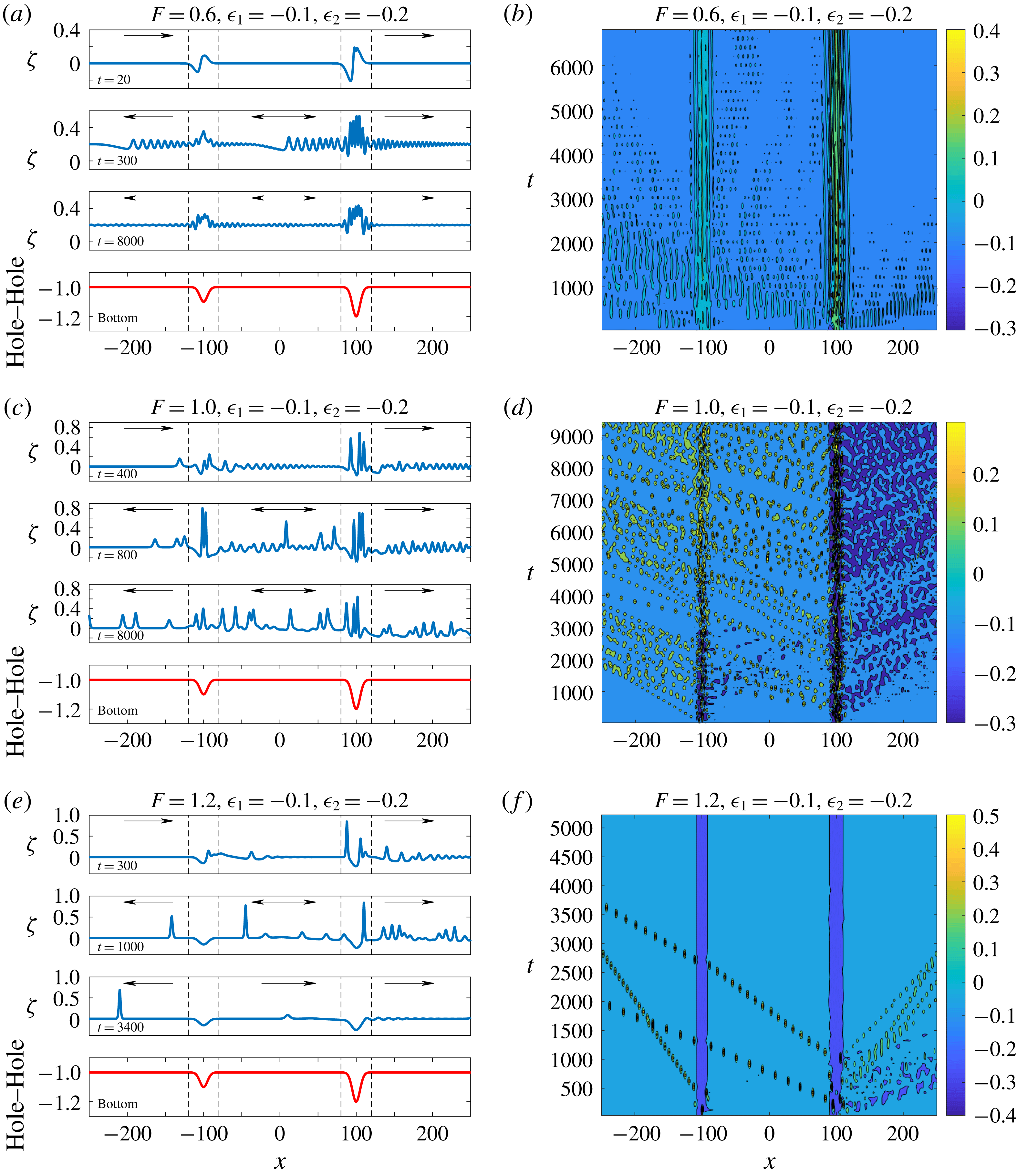
. The case of two holes is shown in figures 4, 5 and 6 for
 $\unicode[STIX]{x1D716}_{1}=-0.1$
,
 $\unicode[STIX]{x1D716}_{2}=-0.01,-0.1,-0.2$
respectively, and for
 $F=0.6,1,1.2$
in each figure, top to bottom panels. The three cases represent the second hole being smaller, of the same magnitude or larger respectively, while
 $\unicode[STIX]{x1D6E5}_{c}=0.39$
for the first hole, and
 $\unicode[STIX]{x1D6E5}_{c}=0.12,0.39,0.554$
respectively for the second hole.
Hole–hole,
 $\unicode[STIX]{x1D716}_{1}=-0.1$
,
 $\unicode[STIX]{x1D716}_{2}=-0.01$
; A (a,b)
 $F=0.6$
, B (c,d)
 $F=1.0$
, C (e,f)
 $F=1.2$
;
 $w=50$
.

Hole–hole,
 $\unicode[STIX]{x1D716}_{1}=-0.1$
,
 $\unicode[STIX]{x1D716}_{2}=-0.1$
; A (a,b)
 $F=0.6$
, B (c,d)
 $F=1.0$
, C (e,f)
 $F=1.2$
;
 $w=50$
.

Hole–hole,
 $\unicode[STIX]{x1D716}_{1}=-0.1$
,
 $\unicode[STIX]{x1D716}_{2}=-0.2$
; A (a,b)
 $F=0.6$
, B (c,d)
 $F=1.0$
, C (e,f)
 $F=1.2$
;
 $w=50$
.

Figure 4 (
 $\unicode[STIX]{x1D716}_{2}=-0.01$
) shows case A (a,b) when the flow is subcritical for both holes, although very close to the transcritical boundary for the first hole, case B (c,d) when the flow is transcritical for both holes, and case C (e,f) when the flow is transcritical for the first hole but supercritical for the second hole. As expected, the first hole regime dominates the evolution since it has much the greater magnitude. In the subcritical case A a slightly oscillatory elevation develops over both holes, much larger over the first hole, and a small-amplitude lee wave field develops behind the first hole and extends past the second hole. In the transcritical case B, as expected, an unsteady elevation forms over the first hole, modulated by the generation of upstream and downstream undular bores. These are more structured than those shown in figure 3 as here the width
 $w=50$
much narrower than
 $w=10\,000$
in figure 3, which emphasises the controlling effect of the linear dispersion more. A similar structure of smaller amplitude develops over the second hole. The downstream undular bore from the first hole interacts with the waves generated at the second hole and continues downstream considerably modulated. On the other hand the upstream undular bore from the second hole is not affected by the first hole up to the end of the simulation. In case C, there is no influence of the waves generated at the second hole as these are swept downstream. At the first hole the flow is still transcritical, a steady depression forms over the hole, an upstream solitary wave is emitted, and a small amplitude rather irregular wave train is emitted downstream, only minimally affected by the second hole.
Figure 5 shows the same three cases A, B, C as in figure 4 but now with
 $\unicode[STIX]{x1D716}_{2}=-0.1$
, the same magnitude as at the first hole. Case A is similar to that in figure 4 and is again subcritical, but close to the transcritical boundary for both holes. There is increased oscillatory behaviour over the second hole, now comparable to that over the first hole. In the transcritical case B the downstream undular bore form the first hole interacts strongly with the upstream undular bore from the second hole, and this interaction extends to upstream of the first hole and downstream of the second hole. In case C the flow at both holes is transcritical, solitary waves are emitted upstream, and that from the second hole passes over the first hole with only a small modification. Figure 6 is a similar case to that in figure 5, and although there is a larger magnitude
 $\unicode[STIX]{x1D716}_{2}=-0.2$
at the second hole than that at the first hole, the evolution is essentially the same. But note that in case A the flow is now transcritical at the second hole, albeit close to the subcritical boundary, so that an upstream undular bore is emitted, which is modulated at the first hole.
3.3 Hole and obstacle
$(\unicode[STIX]{x1D716}_{1}<0,\unicode[STIX]{x1D716}_{2}>0)$

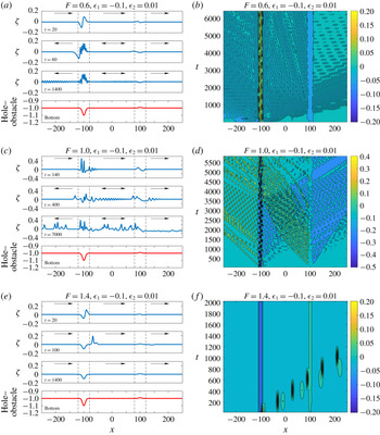
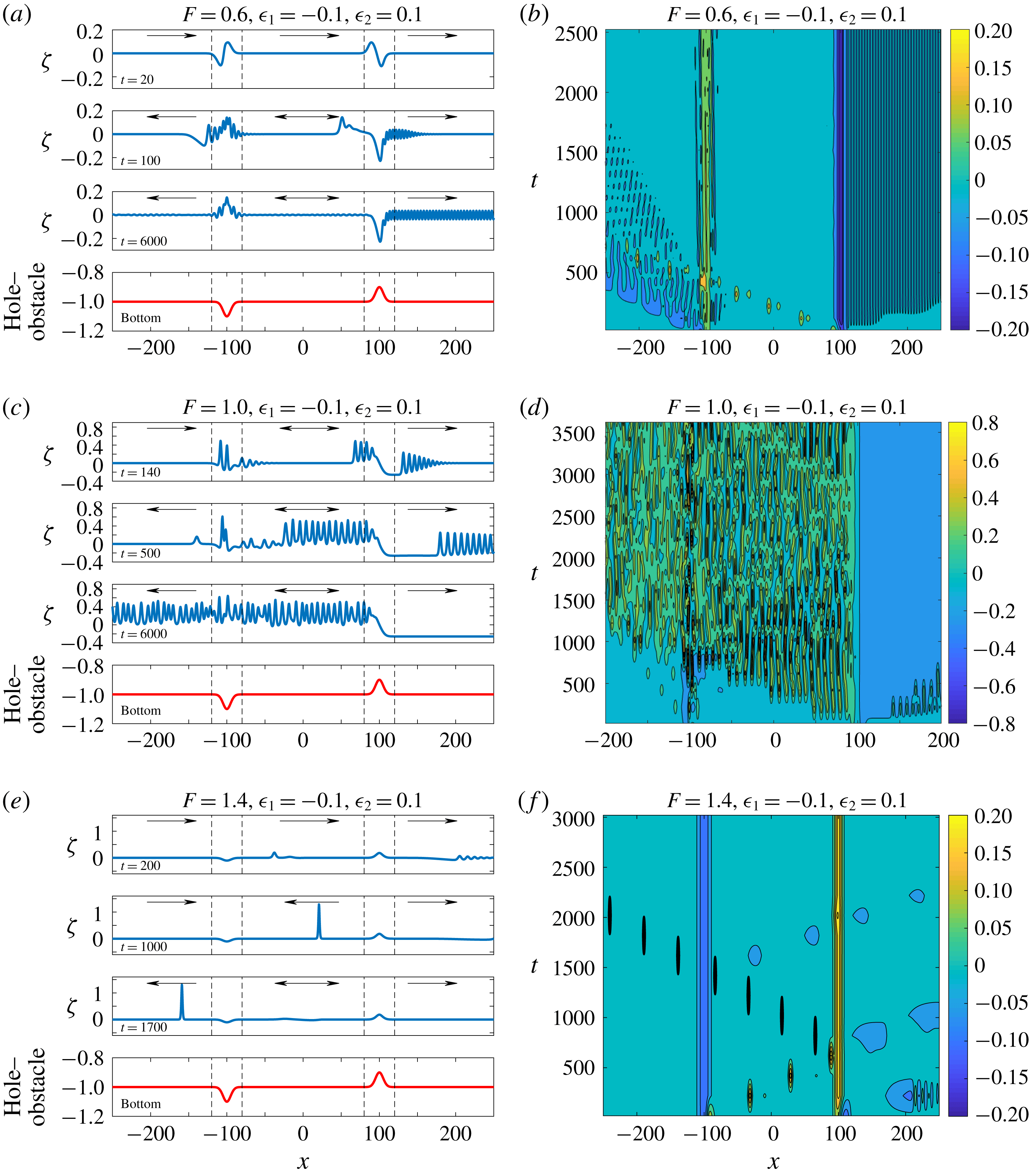
The case of a hole followed by an obstacle is shown in figures 7, 8 and 9 for
 $\unicode[STIX]{x1D716}_{1}=-0.1$
and
 $\unicode[STIX]{x1D716}_{2}=0.01,0.1,0.2$
respectively, and
 $F=0.6,1,1.4$
, while
 $\unicode[STIX]{x1D6E5}_{c}=0.39$
for the hole, and
 $\unicode[STIX]{x1D6E5}_{c}=0.12,0.39,0.554$
for the obstacle. For case A
 $F=0.6$
, the flow is subcritical over the hole so that trapped oscillatory elevation waves occur there. The flow is also subcritical over the obstacle for
 $\unicode[STIX]{x1D716}_{2}=0.01,0.1$
and so a steady trapped depression wave is generated there, but is transcritical for
 $\unicode[STIX]{x1D716}=0.2$
so that the steady depression is accompanied by a lee wave field, which is also evident for
 $\unicode[STIX]{x1D716}_{2}=0.1$
. In case A there is minimal interaction between the hole and the obstacle. For case B
 $F=1$
the flow is transcritical for all hole and obstacle magnitudes. Oscillatory waves are generated over the hole, with upstream and downstream undular bores while a steady hydraulic flow develops over the obstacle with an upstream undular bore and a downstream depression. For all
 $\unicode[STIX]{x1D716}_{2}=0.01,0.1,0.2$
there is an interaction between the downstream undular bore from the hole and the upstream undular bore from the obstacle, increasing in intensity as
 $\unicode[STIX]{x1D716}_{2}$
increases and modulating the flow upstream of the hole and downstream of the obstacle, in the latter case suppressing the downstream waves. For case C
 $F=1.4$
, the flow is supercritical over the hole so that a steady depression wave forms over the hole, and emission of a solitary wave downstream. The flow is also supercritical over the obstacle for
 $\unicode[STIX]{x1D716}_{2}=0.01$
and so a steady small-amplitude elevation wave forms there, with emission of very small-amplitude waves downstream. Although the flow is supercritical for
 $\unicode[STIX]{x1D716}_{2}=0.1$
it is close to the transcritical boundary and so there is an emergence of a solitary wave propagating upstream from the obstacle, which passes over the hole. At the same time the downstream solitary from the hole is partially reflected at the obstacle, and the reflected back again at the hole. The flow is transcritical at the obstacle for
 $\unicode[STIX]{x1D716}_{2}=0.2$
and dominated by the generation of an upstream undular bore, with only minimal interaction with the waves generated by the hole.
Hole–obstacle,
 $\unicode[STIX]{x1D716}_{1}=-0.1$
,
 $\unicode[STIX]{x1D716}_{2}=0.01$
; A (a,b)
 $F=0.6$
, B (c,d)
 $F=1.0$
, C (e,f)
 $F=1.4$
;
 $w=50$
.

Hole–obstacle,
 $\unicode[STIX]{x1D716}_{1}=-0.1$
,
 $\unicode[STIX]{x1D716}_{2}=0.1$
; A (a,b)
 $F=0.6$
, B (c,d)
 $F=1.0$
, C (e,f)
 $F=1.4$
;
 $w=50$
.

Hole–obstacle,
 $\unicode[STIX]{x1D716}_{1}=-0.1$
,
 $\unicode[STIX]{x1D716}_{2}=0.2$
; A (a,b)
 $F=0.6$
, B (c,d)
 $F=1.0$
, C (e,f)
 $F=1.4$
;
 $w=50$
.

3.4 Obstacle and hole
$(\unicode[STIX]{x1D716}_{1}>0,\unicode[STIX]{x1D716}_{2}<0)$

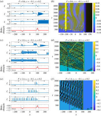
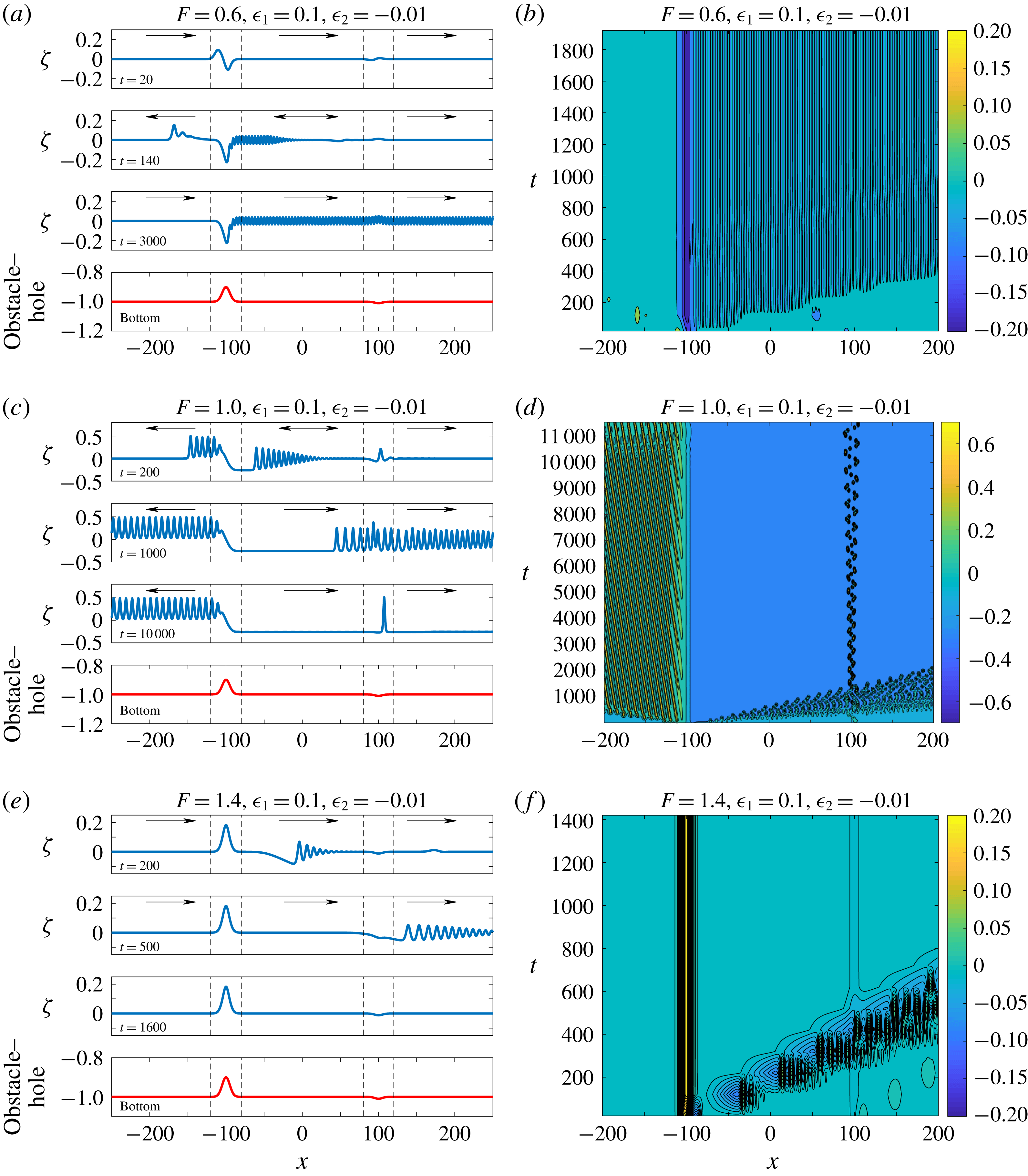
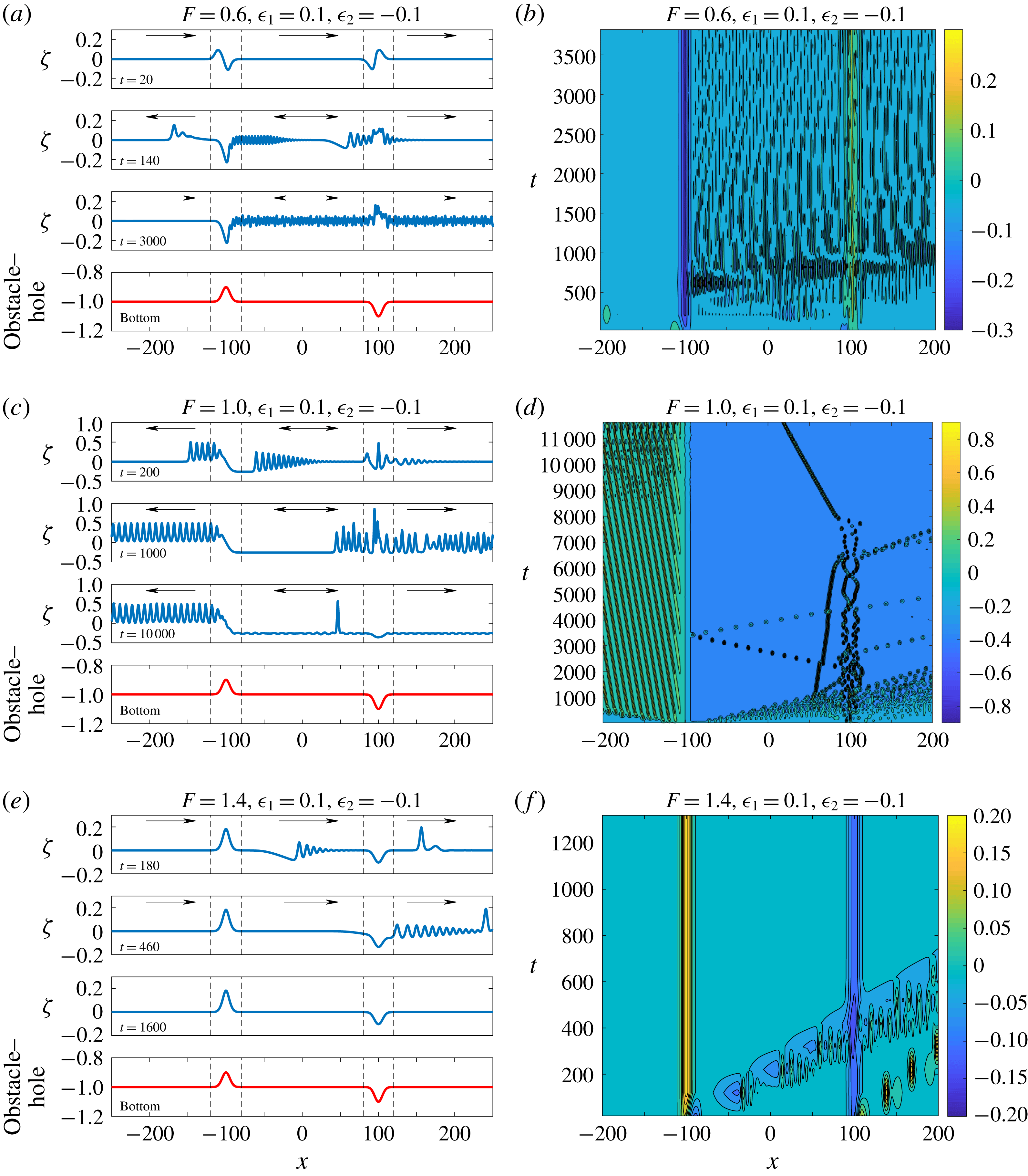
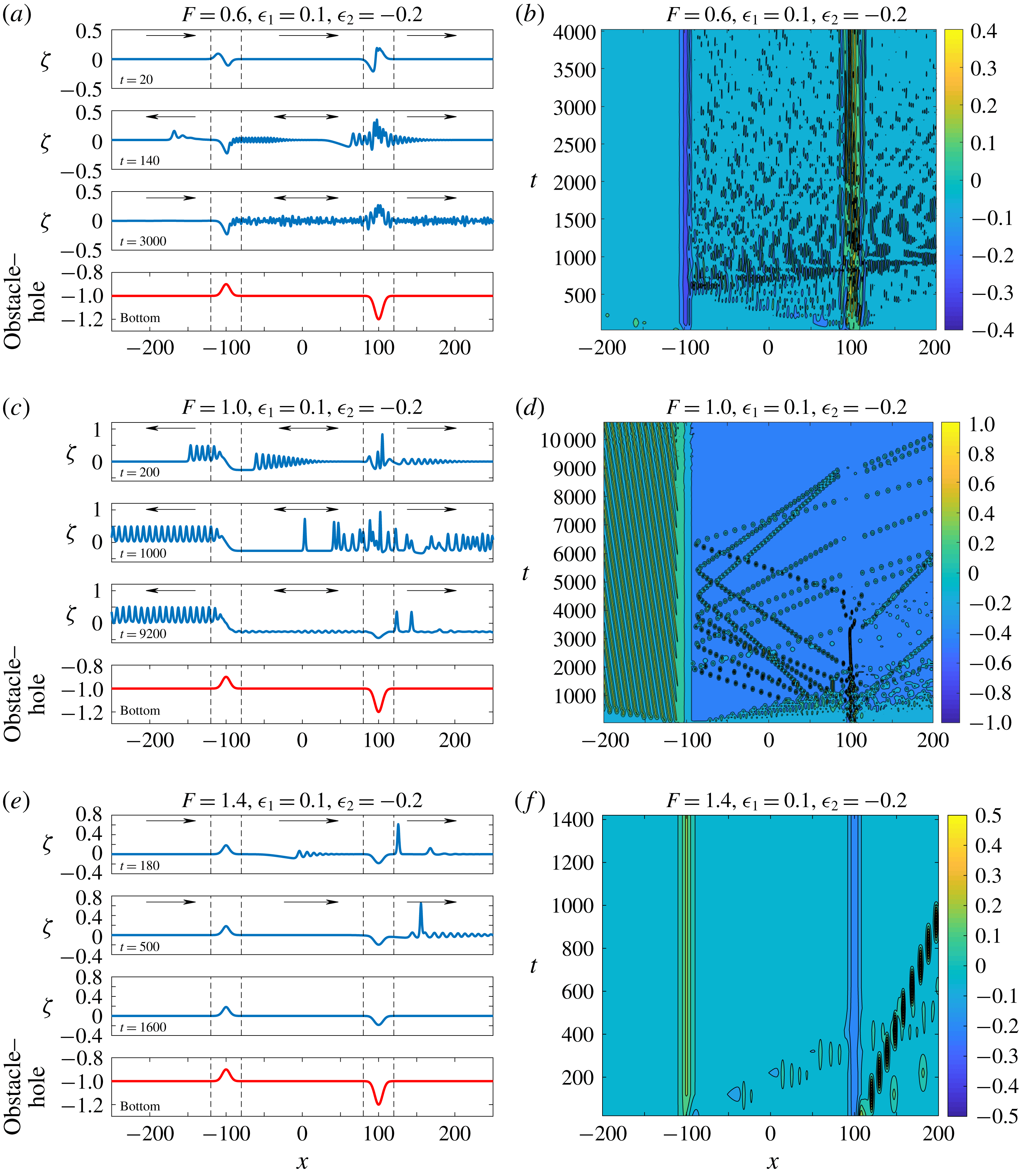
The case of an obstacle followed by a hole is shown in figures 10, 11 and 12 for
 $\unicode[STIX]{x1D716}_{1}=0.1$
and
 $\unicode[STIX]{x1D716}_{2}=-0.01,-0.1,-0.2$
respectively, and
 $F=0.6,1,1.4$
, while
 $\unicode[STIX]{x1D6E5}_{c}=0.39$
for the obstacle, and
 $\unicode[STIX]{x1D6E5}_{c}=0.12,0.39,0.554$
for the hole. For case A
 $F=0.6$
, the flow is subcritical over the obstacle, but close to the transcritical boundary, so a steady depression wave occurs there with downstream lee waves. The flow is also subcritical over the hole for
 $\unicode[STIX]{x1D716}_{2}=-0.01$
but the steady elevation wave and downstream lee waves are suppressed by the lee waves from the obstacle. The flow is subcritical for
 $\unicode[STIX]{x1D716}_{2}=-0.1$
, but close to the transcritical boundary, so that now there is an elevation wave over the obstacle, emission of both upstream and downstream waves, all strongly modulated by the downstream waves from the obstacle. A similar scenario emerges for
 $\unicode[STIX]{x1D716}_{2}=-0.2$
, when the flow is transcritical. For case B
 $F=1$
the flow is transcritical for all obstacle and hole magnitudes. A steady hydraulic flow develops over the obstacle, with an upstream undular bore and a rather weak downstream wave. For
 $\unicode[STIX]{x1D716}_{2}=-0.01,-0.1$
there is an unsteady elevation wave over the hole, and the emergence of upstream and downstream undular bores, but very little interaction with the waves emitted from the obstacle. However, for
 $\unicode[STIX]{x1D716}_{2}=-0.2$
the upstream waves from the hole are reflected at the obstacle, and a more complicated wave field develops. For case C
 $F=1.4$
the flow is supercritical for the obstacle, and a steady elevation forms over the obstacle with the emission of a downstream solitary wave. For
 $\unicode[STIX]{x1D716}_{2}=-0.01,-0.1$
the flow over the hole is also supercritical, and so an oscillatory depression wave forms over the hole, with some downstream waves. For
 $\unicode[STIX]{x1D716}_{2}=-0.01$
these are too weak to affect the waves emitted at the obstacle, and even for
 $\unicode[STIX]{x1D716}=-0.1$
there is only a small and transient interaction. Although when
 $\unicode[STIX]{x1D716}_{2}=-0.2$
the flow is transcritical it is close to the supercritical boundary, the scenario is similar to that for
 $\unicode[STIX]{x1D716}_{2}=-0.1$
.
Obstacle–hole,
 $\unicode[STIX]{x1D716}_{1}=0.1$
,
 $\unicode[STIX]{x1D716}_{2}=-0.01$
; A (a,b)
 $F=0.6$
, B (c,d)
 $F=1.0$
, C (e,f)
 $F=1.4$
;
 $w=50$
.

Obstacle–hole,
 $\unicode[STIX]{x1D716}_{1}=0.1$
,
 $\unicode[STIX]{x1D716}_{2}=-0.1$
; A (a,b)
 $F=0.6$
, B (c,d)
 $F=1.0$
, C (e,f)
 $F=1.4$
;
 $w=50$
.

Obstacle–hole,
 $\unicode[STIX]{x1D716}_{1}=0.1$
,
 $\unicode[STIX]{x1D716}_{2}=-0.2$
; A (a,b)
 $F=0.6$
, B (c,d)
 $F=1.0$
, C (e,f)
 $F=1.4$
;
 $w=50$
.

4 Discussion
In this paper we have extended the study by Grimshaw & Maleewong (Reference Grimshaw and Maleewong2016) for flow over two obstacles using the forced KdV equation (2.1), to flow over two widely separated holes, or to a combination of a hole and an obstacle. Importantly, we again note that for stratified fluids, the terminology obstacle or hole can be reversed and depends instead on the relative polarity of the forcing term and the solitary wave solutions in the absence of any forcing; see Grimshaw & Helfrich (Reference Grimshaw and Helfrich2018). In particular for a stratified fluid with a near-surface pycnocline tidal flow over two bottom ridges, is equivalent in the present setting of the canonical forced KdV equation (2.1) to flow over two holes.
As in the previous study Grimshaw & Maleewong (Reference Grimshaw and Maleewong2016) we find that the flow development can be defined in three stages. In the first stage there is the well-known development of undular bores upstream and downstream of each forcing site, with no interference from the other forcing site, where there is either an unsteady wave pattern for a hole, or a steady hydraulic solution for an obstacle. In the second stage there is an interaction between the undular bore moving downstream from the first forcing site and the undular bore moving upstream from the second forcing site. In the third stage at very large times, there is evolution of this interaction, when one of the forcing sites controls criticality. For unequal forcing magnitudes, the larger magnitude site controls criticality, but for equal forcing magnitudes, either one of the sites can control criticality. This classification holds for all combinations of obstacles and holes.
The previous study Grimshaw & Maleewong (Reference Grimshaw and Maleewong2016) was supplemented by a previous analogous study by Grimshaw & Maleewong (Reference Grimshaw and Maleewong2015) using the fully nonlinear but non-dispersive shallow water equations, and the overall conclusion concerning criticality was unchanged. Although the counterpart for the present combination of holes and obstacles has yet to be carried out, we would expect overall similar conclusions. Also, analogous studies using the fully nonlinear Euler equations have yet to be performed, but based on favourable comparisons between the fKdV model (2.1) and Euler equation simulations for a single forcing, see Grimshaw & Helfrich (Reference Grimshaw and Helfrich2018) and some of the references cited there, we would again expect similar results to emerge.
Next we note that the initial condition in our numerical experiments corresponds to turning on the forcing abruptly at
 $t=0$
. But we recall that the time variable
 $t$
in the forced KdV equation is a slow time, that is
 $\unicode[STIX]{x2202}/\unicode[STIX]{x2202}t\sim \unicode[STIX]{x1D6FC}^{3}$
, and this abrupt introduction of the forcing is in fact a representation of ramping up the forcing on a short time scale. On this short time scale, some small transients will be generated which move rapidly away from the forcing region. This type of introduction of the forcing through an initial condition is easily realisable in a full Euler simulation, and can also be realised in a laboratory setting using a Galilean transformation, that is, moving the forcing up to a speed
 $U$
over a very short time interval
 $t=0$
. But in the ocean for surface and internal waves generated by current flow over bottom topography clearly a different initial condition is needed. Instead the background flow needs to be ‘turned on’. This was examined by Grimshaw & Helfrich (Reference Grimshaw and Helfrich2018) in the case of a tidal flow. Here, we have examined this issue through simulations of the forced KdV equation (2.1) in which the Froude number
 $F$
is increased from zero to a specified constant value, which is then fixed thereafter. The simulation results are very similar to those discussed above in this paper in which
 $F$
is fixed for all time, and the forcing is turned on at
 $t=0$
, except for small transient disturbances which propagate rapidly away from the forcing region. In particular the final stage 3 is unchanged.
Finally we note that we have examined here cases when the forcing sites are widely separated, so that the three-stage evolution of the wave field can be clearly seen. If the forcing sites are instead placed closer together, or even merged into a single site with asymmetric structure, then we would expect to see a merging of the first two stages of the wave field evolution, but the precise outcome needs further exploration, and is beyond the scope of this present work.
Appendix A. Pseudo-spectral numerical method
The forced Korteweg–de Vries (2.1) with initial condition (2.2) is solved numerically using a pseudo-spectral method. The computational domain is periodic over
 $-L<x<L$
, with
 $L=7000$
. The forcing
 $f(x)$
is specified by (3.1). Since the boundary conditions are periodic, we insert a sponge layer in (2.1) by inserting a term,
 $s(x)$
, to absorb small waves approaching the boundaries,
 $$\begin{eqnarray}\displaystyle & \displaystyle -\unicode[STIX]{x1D701}_{t}-\unicode[STIX]{x0394}\unicode[STIX]{x1D701}_{x}+\frac{3}{4}(\unicode[STIX]{x1D701}^{2})_{x}+\frac{1}{6}\unicode[STIX]{x1D701}_{xxx}+\frac{f_{x}}{2}-s(x)\unicode[STIX]{x1D701}=0, & \displaystyle\end{eqnarray}$$
 $$\begin{eqnarray}\displaystyle & \displaystyle s(x)=\frac{\unicode[STIX]{x1D708}}{2}[\{1+\tanh (\unicode[STIX]{x1D705}(x-K/2))\}\{1-\tanh (\unicode[STIX]{x1D705}(x+K/2))\}]. & \displaystyle\end{eqnarray}$$
Here we set
 $\unicode[STIX]{x1D708}=5$
,
 $\unicode[STIX]{x1D705}=0.002$
and
 $K=6500$
. The fKdV equation (A 1) is solved numerically using a combination of a finite different method in time and a Fourier pseudospectral method in space. That is, we write (A 1) as
 $$\begin{eqnarray}\displaystyle \unicode[STIX]{x1D701}_{t}=M(\unicode[STIX]{x1D701})=-\unicode[STIX]{x1D6E5}\,\unicode[STIX]{x1D701}_{x}+\frac{3}{4}(\unicode[STIX]{x1D701}^{2})_{x}+\frac{1}{6}\,\unicode[STIX]{x1D701}_{xxx}+\frac{1}{2}\,f_{x}-s(x)\unicode[STIX]{x1D701}. & & \displaystyle\end{eqnarray}$$
Then we apply the fourth-order Runge–Kutta method,
 $$\begin{eqnarray}\displaystyle \left.\begin{array}{@{}l@{}}\unicode[STIX]{x1D701}^{n+1}=\unicode[STIX]{x1D701}^{n}+\frac{1}{6}\{M_{1}+2M_{2}+2M_{3}+M_{4}\},\\ M_{1}=M(\unicode[STIX]{x1D701}^{n}),M_{2}=M(\unicode[STIX]{x1D701}^{n}+M_{1}/2),M_{3}=M(\unicode[STIX]{x1D701}^{n}+M_{2}/2),M_{4}=M(\unicode[STIX]{x1D701}^{n}+M_{3}),\end{array}\right\}\quad & & \displaystyle\end{eqnarray}$$
where the superscript
 $n$
refers to the time step. We summarise the main steps as follows.
(i) Given
 $\unicode[STIX]{x1D701}_{j}^{n}=\unicode[STIX]{x1D701}(x_{j},t_{n})$
, the derivatives of the linear terms are calculated in the spectral space.
(ii) The nonlinear term is calculated similarly, that is, we get
 $\unicode[STIX]{x1D701}(x_{j},t_{n})$
at each grid point
 $x_{j}$
, then find
 $\unicode[STIX]{x1D701}(x_{j},t_{n})^{2}$
in the physical space.
(iii) Given
 $\unicode[STIX]{x1D6E5}$
, and
 $f(x)$
, we can calculate
 $\unicode[STIX]{x1D701}_{j}^{n+1}$
from (A 4) at
 $x=x_{j}$
and
 $t=t_{n+1}$
.