3.1. Spectral structure of the incident waves and corresponding gap responses

We obtain three sets of undisturbed incident waves ($\eta$) in the absence of the model and the corresponding gap surface elevations ($\varphi$) with the model in place. The measurement lasts until the wave field is contaminated by reflected waves from the side walls of the wave tank. Spectral analysis is conducted on the undisturbed and response surface elevations, to facilitate the demonstration of the different excitation mechanisms. Figure 2 shows the amplitude spectra obtained from the tests of the linear (with the subscript $1\times$), quadratic ($2\times$) and cubic ($3\times$) wave excitations, respectively. It is worth noting that only the first few odd gap modes are excited due to the symmetry of the experimental set-up. The subplots above the spectral peaks in figure 2 demonstrate the corresponding mode shapes, with the upper (yellow) and lower (light blue) parts referring to the area above and below the still water level in the gap, respectively.

Figure 2.

Amplitude spectra of the surface elevations at the centre of the gap with and without the model in place. The dotted curves represent the undisturbed waves $\eta$ in the absence of the model, and the solid curves the response surface elevations $\varphi$ with the model in place. Both $\eta$ and $\varphi$ are measured at the same position using the same wave gauge. The subscripts $1\times$, $2\times$ and $3\times$ in the legend denote the linear, quadratic and cubic excitation processes, respectively. The shapes of the gap modes are demonstrated above the corresponding spectral peaks.

The spectra of the undisturbed incident waves (dotted lines) exhibit little nonlinearity, as shown in figure 2. Large responses at the first few gap resonance modes are excited in the linear ($1\times$) case (blue curves), which is not surprising. The most striking observation from figure 2 is that significant surface elevations at the gap resonance modes have been excited in the $2\times$ (red curves) and $3\times$ (dark green curves) cases, much higher in frequency than the main incident wave components. Thus, they must be driven through nonlinear interactions, i.e. frequency doubling and tripling, where the output sum frequencies are close or equal to the frequencies of the gap resonance modes.

3.2. Nonlinear excitation mechanism

To facilitate the analysis, we discuss the nonlinear wave excitation mechanism here. The undisturbed linear surface elevation at the position of the structure can be written as

(3.1)\begin{equation} \eta^{1}=\sum_{j}a_j\exp({\mathrm{i}(2{\rm \pi}{f_j}t+\theta_j)}), \end{equation}

where $a_j$, $f_j$ and $\theta _j$ refer to the amplitude, frequency and phase information of the $j\textrm {th}$ wave component.

Here we simply take the cubic wave excitation as an example. For a Stokes-type expansion, the cubic frequency gap response can be written as a triple product of linear wave components multiplied by the cubic sum-frequency transfer function. This transfer function is a function of the individual frequencies of three linear wave components,

(3.2)\begin{equation} \varphi^{3+}=\sum_{j}\sum_{k}\sum_{l}\mathrm{CTF}(f_j,f_k,f_l)a_ja_ka_l \exp({\mathrm{i}[2{\rm \pi}(f_j+f_k+f_l)t+(\theta_j+\theta_k+\theta_l)]}). \end{equation}

The output frequency of each contribution to the cubic (sum-frequency) gap response is simply the sum of the frequencies of the three linear wave components.

There are two problems associated with evaluating this cubic frequency response: first, the CTF is unknown in general, and secondly, even if it was available, the effort to evaluate the response is $O(N^3)$, where $N$ is the number of components used to define the linear input.

Our assertion, with support being given in § 4, is that this (three-dimensional) cubic transfer function in the tri-frequency space is flat in the two directions away from the sum output frequency direction. Thus, we can write

(3.3)\begin{equation} \mathrm{CTF}(f_j,f_k,f_l) {\approx}\mathrm{CTF}_{\mathrm{flat}}\left(\frac{f_j+f_k+f_l}{3},\frac{f_j+f_k+f_l}{3},\frac{f_j+f_k+f_l}{3}\right)= \mathrm{CTF}_{\mathrm{flat}}(\mathcal{F}), \end{equation}

as the assumed flat form of the transfer function is only a function of a single variable, the output sum frequency, $\mathcal {F}=f_j+f_k+f_l$.

Another simplification of the cubic response term is the efficient identification of the triple product of linear input components. Using the trigonometric expansions for multiple angles, we can replace the cubic amplitude and triple frequency term using

(3.4)\begin{equation} A^3\cos3\varTheta=[(\eta^1)^2-3(\eta^1_{H})^2]\eta^1 \end{equation}

for narrow-banded waves, where $A$ is the local wave amplitude, assumed slowly varying in time, and $\varTheta$ is the local phase (Walker, Taylor & Eatock Taylor Reference Walker, Taylor and Eatock Taylor2004). The subscript $H$ denotes the Hilbert transform. Then we obtain a simple approximation for the cubic response in the form of a frequency convolution

(3.5)\begin{equation} \varphi^{3+}{\approx}\mathrm{CTF}_{\mathrm{flat}}(\mathcal{F}){\circledast}{[(\eta^1)^2-3(\eta^1_{H})^2]\eta^1}. \end{equation}

By analogy, the gap responses driven by other sum-frequency wave excitations are equivalent, e.g. the source terms are $(\eta ^1)^2-(\eta ^1_{H})^2$ for the quadratic response and $[(\eta ^1)^2-(\eta ^1_{H})^2]^2-4(\eta ^1)^2(\eta _H^1)^2$ for the quartic.

3.3. Temporal structure of the frequency harmonics

To better illustrate the nonlinear processes, we examine the frequency harmonics of the gap resonances. In each set of the experiments, we run the same paddle signal four times, but with each input Fourier component being phase shifted at each run. This generates a set of four-wave series, i.e. nominally crest-focused ($0^\circ$), up-crossing ($90^\circ$), trough-focused ($180^\circ$) and down-crossing ($270^\circ$), all with the same linear envelope. The four-phase wave signals are then combined to extract the first four harmonics, i.e. $\eta ^1$, $\eta ^{2+}$, $\eta ^{3+}$ and $\eta ^{4+}$, referring to the terms with frequencies around $f_p$, $2f_p$, $3f_p$ and $4f_p$, respectively. The extracted harmonics are associated with the Stokes-type expansion for nonlinear waves. The same idea holds for the corresponding gap resonant responses and, thus, we can separate the first four gap resonance harmonics $\varphi ^1$, $\varphi ^{2+}$, $\varphi ^{3+}$ and $\varphi ^{4+}$. For the sake of space, we do not repeat the four-phase decomposition theory here, but details can be found in Fitzgerald et al. (Reference Fitzgerald, Taylor, Eatock Taylor, Grice and Zang2014) or Zhao et al. (Reference Zhao, Wolgamot, Taylor and Eatock Taylor2017). We stress that we look at the harmonics in terms of wave frequency, which should be distinguished from the order of the expansion in terms of nonlinearity (steepness).

The first four harmonics of the undisturbed incident wave groups and the gap resonances are extracted through the four-phase decomposition method. The undisturbed wave field is dominated by the linear component with only small second harmonics being visible and, thus, we only show the first two harmonics. However, here we show the gap resonance signal up to the third harmonics, as we are interested in both frequency doubling and tripling. Figure 3 shows the harmonic components in the case of linear excitation. One can see that the second harmonic $\eta ^{2+}_{1\times }$ is much smaller than the linear component $\eta ^{1}_{1\times }$, confirming little nonlinearity in the undisturbed incident wave field. Significant gap resonant responses with a strong beating pattern in time, which is a result of the gap mode interactions, are excited as shown by the linear component $\varphi ^1_{1\times }$ in figure 3. This is not surprising, as the incident wave frequencies are around those of the first few gap resonant modes. The high frequency harmonic signals, which are simply the bound wave harmonics of the linear response, are much smaller than the linear components.

Figure 3.

Harmonics of the undisturbed incident wave groups ($\eta$) and the gap responses ($\varphi$) driven by linear excitation, where the incident wave frequencies fall around the frequencies of the gap resonances. The superscripts 1, $2+$ and $3+$ refer to the linear, second and third sum-frequency harmonics, while the subscript $1\times$ represents the linear wave excitation. The undisturbed and response surface elevations are aligned in time, where $t=0$ s refers to the focal time of the undisturbed crest-focused wave group.

More interesting phenomena are observed in the quadratic excitation (see the beginning of § 3 for definition) shown in figure 4, where the second harmonic response $\varphi ^{2+}_{2\times }$ is as large as the linear component $\varphi ^{1}_{2\times }$, while the third harmonic $\varphi ^{3+}_{2\times }$ is small. The most striking observation is from the cubic excitation shown in figure 5, where a significant third harmonic response is excited. The second harmonic in figure 4 and the third harmonic in figure 5 must be driven through nonlinear processes, i.e. frequency doubling and tripling, respectively, as there is no linear incident wave energy anywhere near the frequencies of the gap modes (see the input spectra in figure 2).

Figure 4.

Same as in figure 3, but for the quadratic excitation (marked as $2\times$).

Figure 5.

Same as in figure 3, but for the cubic excitation (marked as $3\times$). Note the different vertical scales with figure 3. The $\hat {\varphi }$ terms (dotted curves) in the bottom subplot refer to a repeated run with smaller incident wave amplitude. Here $\zeta$=1.61 is the ratio of the linear incident wave amplitudes between these two experiments.

To support the assertion of the frequency tripling process, we repeat the cubic excitation experiment with incident waves of smaller amplitude, i.e. the linear amplitude ratio of the larger incident wave group to the smaller being $\zeta$=1.61. The first and third gap response harmonics (dotted curves) obtained from the smaller wave test are given in figure 5, with each being scaled by $\zeta$ and $\zeta ^3$, respectively. The good agreement between these two sets of experimental results clearly confirms the idea of a frequency tripling process with a cubic dependency on wave amplitude.

Having identified the gap responses driven by frequency tripling, it is an obvious step to explore whether gap resonance can be excited through frequency quadrupling of four linear input components from the low side of the spectral peak. To facilitate the analysis, we provide the spectra of the first four gap response harmonics obtained from the cubic experiment in figure 6(a). The fourth harmonic spectrum (purple curve) shows local peaks in the frequency range 1.0 to 1.2 Hz, corresponding to the gap mode frequencies. We would expect the fourth harmonic signals to obey the same scaling relation between the two experiments of different input wave amplitudes. Figure 6(b) shows the fourth harmonics where the one from the smaller wave test is amplified by a coefficient of $\zeta ^4=1.61^4$. The amplitude and general shape of these two curves match well, although a slight phase shift is observed. There is probably some contribution to the fourth harmonic response from the simple double frequency bound wave of the frequency doubled gap response as well as a direct quartic response via the local combination of four linear components. It is worth noting that the magnitude of the fourth harmonic response in the smaller wave test is extremely small, i.e. ${\sim }$0.3 mm, and, thus, the slight phase misalignment is somewhat unsurprising. Given the discussion above, we believe most of the gap resonance signal ${\varphi }^{4+}_{3\times }$ shown in figure 6 is excited by a frequency quadrupling process.

Figure 6.

Same (cubic excitation) tests as in figure 5, but focusing on the fourth harmonics. (a) Spectra of the harmonic components in the cubic excitation test (with larger incident wave amplitude). (b) The fourth harmonics of the gap responses, where the one obtained from the smaller wave test $\hat {\varphi }^{4+}_{3\times }$ is amplified by $\zeta ^4=1.61^4$.

The gap resonances, no matter how they have been driven, e.g. linearly, quadratically, cubically or quadruply by compact wave groups, show very similar profiles in time – decaying slowly with similar beating patterns. The slowly decaying process is associated with the weak radiation (wave energy ‘escaping’ from the gap) and small viscous damping for narrow gaps. The beating pattern is a simple interference of the first few gap modes.

4.1. Geometric similarity in nonlinear transfer functions

The overall gap resonances driven through different mechanisms show very similar behaviour, as demonstrated by the normalised (by their maxima) time histories plotted together in figure 7. The linearly excited gap resonance is not shown for comparison here, because the duration of the excitation by the linear wave group is much longer in time. The gap resonance time history in the quadratic excitation agrees very well with that in the cubic excitation. The one excited through frequency quadrupling agrees slightly less well here, simply because the centre frequency of the input wave group is chosen to excite the cubic interactions efficiently. We would expect to get a better match for the four-wave excitation of the gap with a lower centre frequency. Now we provide some discussion as to why the gap resonances driven through different mechanisms behave so similarly.

Figure 7.

Normalised (by their maxima) gap resonances driven through different nonlinear mechanisms, i.e. frequency doubling ($\varphi ^{2+}_{2\times }$), tripling ($\varphi ^{3+}_{3\times }$) and quadrupling ($\varphi ^{4+}_{3\times }$) processes. Note the $\varphi ^{2+}_{2\times }$ signal is shifted towards the left by 1 s ($\sim$ one gap period), to align with the $\varphi ^{3+}_{3\times }$ signal at the response peak.

It is convenient to use the term $n$-TF for the quadratic, cubic and quartic transfer functions, with $n=2$, 3 and 4 for what we are calling QTF, CTF and Q$^4$TF, respectively. The responses of the gap driven nonlinearly can be written as a $n$-multiple integral over the $n$-TF $\times$ $n$-products of linear wave components, e.g. (3.2) for the cubic case. Of course, we note that no general diffraction code is currently available for $n>2$, yet we aim to provide a method for approximating gap resonances for $n=3$ and 4. For the tests, the incident wave group is ‘focused’, so at relative time of zero the phases of all the incident linear components are very close to zero. The phase of the $n{\mathrm {th}}$ harmonic bound wave, approximated as the $n$-products of linear wave components, should also be zero. The spectra of the groups are Gaussian in form. In terms of output sum-frequency variation across the gap mode frequencies of interest, i.e. the first to third gap modes, the excitation is close to ‘flat’. As far as the gap mode frequencies are concerned, the excitation is zero phase and flat in frequency, so approximates to an impulse excitation. It is therefore expected that the mode response is essentially the impulse response of the gap, and that the variation in time of the gap response should be the same irrespective of whether the excitation is quadratic or cubic. However, we would expect to see some difference for the quartic case as the excitation, estimated from four-wave combination towards the low frequency tail of the input spectrum, is not completely flat in output frequency and, thus, the first three gap modes ($m=1$, 3, 5) are not equally excited.

The $n$-TFs must reflect the output resonant behaviour of the gap – lightly damped resonant peaks at each of the gap modes. Hence, the $n$-TFs will have strong variation along the output frequency ($n$-sum of linear input frequencies) direction, but little if any variation in all other directions perpendicular to this. We can then approximate the $n$-TF in terms of a one-dimensional form along the leading diagonal which is flat in all directions perpendicular to this, e.g. (3.3) for $n=3$. As a result, apart from a simple constant scaling factor for each $n$-TF, we would expect the modal excitation in the gap to be simply the $n$-product of the linear incident wave components combined with the transfer functions in the output frequency direction. If the assumption introduced above is correct, we would then expect that the relative amplitude and phase for all the $n$-TFs should look the same, along the output frequency direction.

Based on the measured data, we calculate the LTF and approximate the sum-frequency quadratic, cubic and quartic transfer functions for gap responses. The LTF is obtained simply through the ratio of the spectra between the linear gap response and the linear incident wave, both being extracted through the four-phase decomposition of the measured data, as in Zhao et al. (Reference Zhao, Wolgamot, Taylor and Eatock Taylor2017). The $n$-TFs are simply approximated as the LTF between the $n{\mathrm {th}}$ harmonic of the gap response $\varphi ^{n+}$ and the $n$-product of the linear waves $\eta ^1$, e.g. (3.4) for $n=3$. Both the $\eta ^1$ and $\varphi ^{n+}$ time histories are obtained through the four-phase decomposition of the measured data. We are using the estimated $n$-linear wave approximation for the $n{\mathrm {th}}$ harmonic, because it represents a simple model which makes it possible to predict the $n{\mathrm {th}}$ harmonic excited gap response once the linear input and the $n$-TFs are given.

Figure 8 shows the transfer functions for $n=1$, 2, 3 and 4, as high in frequency as our experiments allow us to go. It is striking that the $n$-TFs with $n>1$ show very much the same shape both in amplitude and phase. Interestingly, the net phase across the $m=1$ gap mode changes by ${\rm \pi}$ and again by another ${\rm \pi}$ for $m=3$. This is consistent with a series of simple one-degree-of-freedom systems, where the phase of the output changes by ${\rm \pi}$ across each resonance. The LTF shows a similar shape in amplitude, but with the relative phase being different to that of the CTF. This may be relevant to the details of the excitation process going from the incident waves to the forcing of the gap modes. For the linear excitation ($n=1$), the wavelength of the incident wave is of the same order of magnitude as the length of the gap. Hence, the local waves are significantly diffracted. This is different to the $n>1$ cases, where the incident free-wave wavelength is $n^2\times$ the scale required to drive the gap linearly, so less linear diffraction will occur. The phase for odd order transfer functions is ${\rm \pi}$ for frequencies below the first ($m=1$) gap mode, whereas it is 0 for the even order transfer functions. This is consistent with the forcing process, i.e. $(-1)^n\times n$-product of linear terms.

Figure 8.

Transfer functions of the surface resonant responses at the centre of the gap with broadside wave incidence, (a) amplitude for the linear and cubic transfer functions, (b) amplitude for the quadratic and quartic transfer functions, (c) phase for linear and cubic transfer functions, and (d) phase for the quadratic and quartic transfer functions. The non-dimensional transfer functions are written as $\varphi ^{n+}/L=n\text {-}\textrm {TF}{\circledast }(\eta ^1/L)^n$, so that they are independent of the length ($L$) of the model. Here ‘Q$^4\textrm {TF}$’ in the legends refers to the quartic transfer function, and the integers 4, 9 and 60 are simply chosen to match the amplitudes of the transfer functions at the $m=1$ mode. Note the phase difference ${\rm \pi}$ between the phases of (c,d), and the horizontal axis $f$ refers to output frequency in these plots.

Given the good similarity between the geometric shapes of these transfer functions, it might be possible to deduce the quadratic, cubic and quartic transfer functions of gap resonances based on as simple as linear-type transfer functions, which would greatly reduce the computational effort. The good similarity, together with the discussion above, supports that the higher-order transfer functions, e.g. CTF in tri-frequency space, should show similar geometric characteristics to the sum-frequency QTF in a bi-frequency plane.

4.2. Near-flat form of gap surface QTF – potential flow calculation

It is possible to calculate the full sum QTF matrix for the gap resonant responses, but it is not clear that it is feasible to calculate the full sum matrices for the cubic and quartic transfer functions. As a consequence, we focus on examining the structure of the sum-frequency QTF matrix here. To achieve this, we calculate the gap response between the two fixed structures (for the configuration in figure 1), by neglecting viscous damping.

The potential flow code DIFFRACT has been used for the numerical simulations. A detailed description of the relevant theory can be found in Chau & Eatock Taylor (Reference Chau and Eatock Taylor1992) and Sun, Eatock Taylor & Taylor (Reference Sun, Eatock Taylor and Taylor2015), and verification of this programme has been demonstrated in previous publications, e.g. Sun et al. (Reference Sun, Eatock Taylor and Taylor2010). Numerical and grid convergence has been confirmed for the results presented here. It is well known that the free-surface elevation at the second order can be written as (see Malenica, Eatock Taylor & Huang (Reference Malenica, Eatock Taylor and Huang1999) for example)

(4.1)\begin{equation} \eta^{(2)}={-}\frac{1}{g}\left[\frac{\partial\phi^{(2)}}{\partial t}+\frac{1}{2}\boldsymbol{\nabla}\phi^{(1)}\boldsymbol{\cdot}\boldsymbol{\nabla}\phi^{(1)}-\frac{1}{g}\frac{\partial \phi^{(1)}}{\partial t}\frac{\partial^2\phi^{(1)}}{\partial z \partial t}\right]. \end{equation}

There is a natural separation into potential and quadratic terms to facilitate the interpretation of computed results; see Molin (Reference Molin1979) and Kim & Yue (Reference Kim and Yue1990), for example. In the present case, as in Malenica et al. (Reference Malenica, Eatock Taylor and Huang1999), the resonant response is associated with the potential contribution (the first term in (4.1)).

The sum-frequency QTF matrix of the gap response is calculated at the centre of the gap with broadside wave incidence. We focus on the leading diagonal terms in the bi-frequency plane, by looking at frequency pairs $(f_j,f_k)$ where $j=k$. Figure 9(a) shows the calculated gap surface QTF (modulus) along the leading diagonal. This is very similar in shape to, though larger than, that obtained from the experiments (see figure 8). It is worth noting that the potential flow calculation does not account for any viscous damping, explaining the larger amplitude in the numerical simulations than that from the experiments.

Figure 9.

Second-order sum-frequency surface QTF at the centre of the gap from potential flow calculations. (a) Shows the modulus of the transfer function along the leading diagonal and (b) the off-diagonal QTF terms ($f_j-f_k$) with the corresponding frequency sum ($f_j+f_k$) fixed at the frequencies for the $m=1$, $m=2^*$ and $m=3$ modes, respectively. The blue solid dots are calculated using a truncated mesh with meshed radius of $0.6\times$ gap length, while the remaining are based on a full mesh with meshed radius of $5\times$ gap length. Note $m=2^*$ is simply chosen to be the frequency (1.085 Hz) at which the QTF is a minimum between $m=1$ and $m=3$ modes, as the gap centre is a node for the $m=2$ mode which would not be excited in this symmetric configuration.

Here we take advantage of numerical simulations to evaluate the relative importance of the free-surface forcing terms in the gap, and outside the gap. By reducing the radius of the surface over which the free-surface terms are integrated, we show that the results are negligibly affected by the outer free-surface integral and dominated by the local forcing. The approximate results in figure 9 indicate the small differences caused by including the outer free surface, and show the flat behaviour of the local forcing. Further, the calculation shows that scattering of the incident second-order potential is negligible at the peaks of the QTF for gap response.

We then explore the off-diagonal terms in the direction perpendicular to the leading diagonal, i.e. varying the frequency difference ($f_j-f_k$) when keeping the frequency sum ($f_j+f_k$) constant, for the $m=1$, $m=2^*$ and $m=3$ modes, respectively. Figure 9(b) clearly shows that the second-order sum-frequency QTF ridge at the $m=1$ mode is approximately constant close to but perpendicular to the leading diagonal. Further away from the leading diagonal, this approximation becomes less reliable. We believe the variation is smaller in the experiments, where viscous damping is included leading to smaller response amplitudes in general. Rather than running as many calculations as for the $m=1$ mode, we run four sets for the $m=3$ mode, showing clearly a close to flat form for the gap surface QTF. It is worth noting that the $m=2^*$ mode here is simply chosen to be the trough between the $m=1$ and $m=3$ modes, as no anti-symmetric modes could be excited in this symmetric configuration and the gap centre is a node for the $m=2$ gap mode.

The second-order potential flow calculation strongly supports the idea that the sum-frequency QTF matrix of gap response, both at and off resonance, has a near-flat form in the direction perpendicular to the leading diagonal in the bi-frequency plane. It is therefore appropriate to assume a ‘flat’ QTF form, so that one can approximate the full sum-frequency QTF matrix based on the leading diagonal terms. We note that a realistic irregular sea state has a high concentration of energy around the spectral peak, and, thus, the quadratic excitation terms are also localized around the leading diagonal.

4.3. Flat QTF approximation

Calculating the full QTF matrix is very time consuming, but the near-flat structure makes it possible to reduce the computational effort greatly. As noted earlier, the sum-frequency QTF of the gap response is a strong function of the output frequency sum ($f_{j}+f_{k}$) and nearly independent of the frequency difference ($f_{j}-f_{k}$).

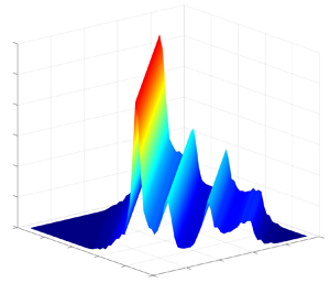
Here, we approximate the full sum QTF matrix by assuming $H_{jk}=H_{kj}=H_{((\,{j+k})/{2})((\,{j+k})/{2})}$ with $H_{((\,{j+k})/{2})((\,{j+k})/{2})}$ being the leading diagonal terms – so a ‘flat’ QTF approximation. As noted, the leading diagonal terms in the QTF matrix could be obtained from the quadratic excitation testing (as shown in figure 4), where the incident wave is a transient wave group with a narrow-band underlying spectrum (see figure 2). These are given in figure 8. Based on the ‘flat’ form approximation, the off-diagonal terms can be easily obtained simply by ‘stretching’ each leading diagonal term along the perpendicular direction. Figure 10 shows the approximated QTF matrix, being ‘flat’ in the perpendicular direction to the leading diagonal in the bi-frequency plane.

Figure 10.

Sum-frequency gap surface QTF matrix based on the ‘flat’ approximation. The upper triangular area is for phase information, while the lower part is for modulus. In this bi-frequency plane the leading diagonal terms produced by $f_j+f_k$ with $j=k$ are the same as in figure 8(b) for modulus (divided by 4) and 8(d) for phase. In the perpendicular direction to it, the off-diagonal terms, produced by $f_j-f_k$ with $f_j+f_k$ being constant, are given in the form of $H_{jk}=H_{kj}=H_{((\,{j+k})/{2})((\,{j+k})/{2})}$, with the latest term being from the leading diagonal. Each dashed line, representing an output frequency sum ($f_j+f_k$), marks the frequency of each gap mode.

The ‘flat’ QTF approximation reduces the number of calculations significantly from ${\sim } N^2/{2}$ to $N$ for a random sea state, where $N$ is the number of linear frequency components used to discretise the wave spectrum. The effectiveness of this approximation is further supported by the experimental data in irregular waves, which is detailed in the following section.

5.1. Gap response driven nonlinearly in irregular waves

A unidirectional sea state with a JONSWAP-type form is generated in the basin to excite gap surface responses for the same set-up as for the transient wave tests in § 2. In the experiment the wave generation lasts for 30 min, with the sea state being characterised by significant wave height $H_s= 0.081$ m, spectral peak frequency $f_p= 0.43$ Hz and peak enhancement parameter $\gamma =5$. This represents a realistic scenario of swells approaching the gap with broadside incidence.

To facilitate the discussion, the time histories and spectra of the undisturbed incident waves ($\eta$) and the gap responses ($\varphi$) are given in figure 11. The undisturbed incident wave energy is distributed within the frequency range 0.3 to 0.85 Hz – lower than the frequencies of the gap modes. As a consequence, there is no linear wave energy input to excite the gap modes of interest, whose frequencies concentrate around 1.0 to 1.3 Hz. It is worth noting that there are still gap responses being excited, i.e. the blue part of $\varphi$ under the incident wave spectrum. These are simply linear responses of the gap surface to the incident waves, where no gap mode is involved – so off resonance. Through frequency doubling, i.e. $2\times [0.3,0.85]=[0.6, 1.7]$ Hz, the gap modes can be well excited at resonance. This explains the large gap responses (red $\varphi$) beyond the incident wave frequency range. By analogy, the frequency tripling process, producing a frequency range $[0.9, 2.55]$ Hz with energy centred at 1.29 Hz, could also contribute to the red part of $\varphi$, though its contribution is expected to be extremely small.

Figure 11.

Time histories and spectra of the surface elevations at the centre of the gap with and without the model in place. The dotted curve represents the undisturbed waves $\eta$ in the absence of the model, and the solid curve the response surface elevations $\varphi$ with the model in place. The blue part of $\varphi$ is driven linearly by the incident waves, while the red part represents those by a nonlinear process. Both $\eta$ and $\varphi$ are measured at the same position using the same wave gauge.

It is straightforward to distinguish the gap responses driven by linear and nonlinear processes for the case here, based on simple digital frequency filtering. However, the frequency overlapping makes it hard to distinguish the relative contributions between frequency doubling and frequency tripling processes, though the former one dominates. Therefore, we run four-phase testing for the irregular waves as for the transient wave group testing in § 3.3, in an attempt to extract the first four harmonics of the gap responses. The separated harmonic signals allow us to examine the performance of the ‘flat’ QTF (and CTF) in detail.

5.2. Harmonic analysis – calculation vs experiment

Similar to the transient wave group tests in § 3.3, four-phase decomposition is conducted for the irregular wave tests, separating the first four harmonics of the undisturbed incident waves and the corresponding gap responses. For the gap responses, it is noted that the higher harmonic responses beyond the third are negligible, with the third harmonic being small. Therefore, we calculate each of the first three harmonics of the gap responses, using the LTF, QTF and CTF, respectively. The QTF matrix is obtained using the ‘flat’ approximation as demonstrated in figure 10, and the CTF matrix is constructed similarly. The second and third gap response harmonics can be estimated in the way discussed in § 3.2, e.g. using (3.2) for the calculation of the third harmonic, while it is straightforward to calculate the linear harmonic here, i.e. a convolution of incident wave signal ($\eta ^1$) and the LTF.

The estimated and experimentally determined harmonics of the gap responses are given in figure 12, together with the undisturbed incident waves. One can see that the undisturbed wave field $\eta$ (with mild steepness $k_pH_s=0.06$) is dominated by the linear component with the second harmonic being negligible. As shown in figure 11, the linear wave energy lies outside the gap resonance frequency range, where the components of LTF (not shown here) are smooth and only slightly varying with frequency, quite different to the strongly structured part (due to gap mode resonances) shown in figure 8(a).

Figure 12.

Harmonics of the surface elevations at the centre of the gap with and without the model in place. The undisturbed waves in the absence of the model are marked as $\eta$, and the response surface elevations with the model in place are marked as $\varphi$. The subscript ‘$e$’ refers to the experimentally determined harmonics, while ‘$c$’ represents the results calculated based on the transfer functions shown in figure 8. Note the different scales in the vertical axes.

The linear gap responses show good agreement, which is not surprising. It is however striking that the estimation of second gap response harmonic based on the ‘flat’ QTF matches well to the experimentally determined result. This supports the assumption that the sum-frequency QTF matrix for gap resonances has a close to flat form in the direction perpendicular to the leading diagonal, in the bi-frequency plane.

The agreement in the third harmonic is less satisfactory, which is to be expected. The irregular waves here produces a peak frequency of 1.29 Hz through frequency tripling, which is outside the major gap mode frequencies interested here and, thus, only triggering weak gap resonances. Extracting such a small harmonic signal is much harder in irregular waves than in the transient wave groups in which all harmonics focus at the same time. The experimentally determined third harmonic of the gap response here is thus expected to be less reliable, compared with the first and second harmonics. Given this, the less satisfactory agreement in the third harmonics seems to be understandable – a rather weak support of ‘flat’ CTF. It is worth emphasizing that this irregular wave testing is designed to drive the gap resonances through frequency doubling, with weak frequency tripling being a ‘bonus’.

5.3. Conditioning analysis: application to linear and nonlinear harmonics

The prior section demonstrates the effectiveness of ‘flat’ QTF on a wave-by-wave basis. Here we are interested in its performance on peak responses on an averaged basis in irregular waves.

We now seek to adopt the NewWave-type concept (Tromans et al. Reference Tromans, Anaturk and Hagemeijer1991; Jonathan & Taylor Reference Jonathan and Taylor1997), to look at the average shape of the large incident wave in time (the so-called NewWave) and the resultant gap responses, similar to our analysis for the tertiary wave-structure interactions in Zhao et al. (Reference Zhao, Taylor, Wolgamot and Eatock Taylor2019). This type of analysis allows us to extract NewWave-type profiles and the associated gap responses from the irregular wave test. As a result, it facilitates the comparison of the irregular wave testing results with the transient wave group tests in § 3.3.

The basic idea of this type of analysis involves constructing NewWave-type profiles (similar to the incident wave record in figure 4) from random signals, e.g. the irregular wave elevations, and the associated response profiles. It is noted in § 5.2 that the undisturbed incident waves show little nonlinearity, so are dominated by linear components, while the gap responses beyond the third harmonics are negligible. Therefore, here we focus on the linear incident wave component (marked as $\eta$ in this section for simplicity) and the linear and second harmonics of the gap responses. A NewWave-type profile is obtained from averaging a given number of the ordered largest profiles in the record, by creating shorter time series with maxima at (relative) time zero. In this study we selected short segments of time history centred at each of the top 15 linear crests in the undisturbed incident wave to obtain the average shape, the so-called NewWave profile ($\eta _{e}$) as shown in figure 13(a).

Figure 13.

NewWave profile of the (linear) undisturbed incident wave surface elevations ($\eta$) in the absence of the model, and the harmonic separation of the corresponding gap responses ($\varphi$) with the model in place. The subscripts ‘$e$’ and ‘$c$’ have the same meaning as in figure 12. The shading represents 95 % confidence intervals on the estimation of the mean signals (the solid black curves).

To obtain the associated gap responses, a conditioning process is introduced when performing the averaging process. The reference times, which are used for selecting the peaks of the undisturbed waves when constructing the NewWave profile, are also used to obtain the corresponding local gap responses. Figure 13(b,c) shows the linear ($\varphi ^1_{e}|\eta _{e}$) and second ($\varphi ^{2+}_{e}|\eta _{e}$) harmonics of the gap responses given the NewWave profile of the incident wave. A flowchart which clearly demonstrates the conditioning process has been given in Zhao et al. (Reference Zhao, Taylor, Wolgamot and Eatock Taylor2019), and, thus, we do not repeat it here. It is worth noting that the process here is relatively straightforward, as the first four harmonics are separated, as shown in § 5.2, based on the four-phase signals obtained from running the same wave paddle signals four times with each Fourier component being shifted at each run.

After obtaining the NewWave profile of the incident wave ($\eta _{e}$), we also calculate the associated gap response harmonics using the LTF and the ‘flat’ QTF. The estimated linear and second harmonics of the gap responses (dotted lines), are compared with the experimentally determined results (black solid lines) in figure 13. Given that the experimentally determined gap surface responses are obtained from an irregular sea excitation with limited duration, the agreement with the estimation is fairly good, though might be improved by increasing the experimental duration. Overall, these results provide some support for the ‘flat’ QTF assumption.

By analogy, we construct the ‘NewResponse’ profiles (average shape of large responses) from the first ($\varphi ^{1}_{e}$) and second ($\varphi ^{2+}_{e}$) harmonics of the gap responses, respectively, and extract the incident wave profiles that give the large responses – the so-called design waves $\eta |\varphi ^{1}_{e}$ and $\eta |\varphi ^{2+}_{e}$ in figure 14. The design waves are then used as input waves to estimate the first and second gap response harmonics, respectively, together with the LTF and ‘flat’ QTF. Figure 14 shows good agreement between the estimated (dotted lines) and experimentally determined (black solid lines) NewResponse profiles – the most probable maximum responses.

Figure 14.

Similar to figure 13, but for the design waves and their produced NewResponse profiles for the linear and second gap response harmonics.

The NewResponse profile $\varphi ^1_{e}$ shows considerable similarity to its design wave $\eta |\varphi ^1_{e}$, though with phase being shifted and amplitude being reduced. This is simply because the LTF is close to be constant (approximately 0.5) across the incident wave frequencies 0.25 to 0.85 Hz as shown in figure 11, where there is no gap resonance.

More interesting phenomena are observed for the second harmonics. The design wave $\eta |\varphi ^{2+}_{e}$ (in figure 14) with amplitude one-quarter of the NewWave $\eta _{e}$ (in figure 13), but with much more critical wave frequency content and phasing, gives rise to the most energetic excitation (the expected maximum gap response), which is now 1.5 times as large. This is a result of the resonant responses of multiple gap modes. Hence, as far as the nonlinear excitation of the gap responses is concerned, the design wave is not the most extreme wave in the incident sea state.

In any future experimental testing or simulations in computational fluid dynamics, the design wave $\eta |\varphi ^{2+}_{e}$ would be an ideal waveform for examining extreme gap responses driven by a nonlinear frequency doubling process.