


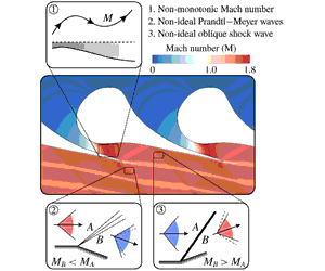


1 Introduction
Flows of molecularly complex fluids in the neighbourhood of the vapour–liquid saturation curve and critical point depart significantly from the ideal-gas-like behaviour typical of dilute thermodynamic states. This discrepancy emerges from the analysis of the sound-speed variation along isentropic transformations, which can be conveniently reduced to the evaluation of the thermodynamic parameter
 $\unicode[STIX]{x1D6E4}$
,
 $$\begin{eqnarray}\unicode[STIX]{x1D6E4}=1+\frac{\unicode[STIX]{x1D70C}}{c}\left(\frac{\unicode[STIX]{x2202}c}{\unicode[STIX]{x2202}\unicode[STIX]{x1D70C}}\right)_{s},\end{eqnarray}$$
known as the fundamental derivative of gas dynamics, see Thompson (Reference Thompson1971). In the above definition,
 $\unicode[STIX]{x1D70C}$
is density,
 $s$
is the specific entropy and
 $c=(\unicode[STIX]{x2202}P/\unicode[STIX]{x2202}\unicode[STIX]{x1D70C})_{s}^{1/2}$
is the speed of sound, in which
 $P$
is the pressure. If
 $\unicode[STIX]{x1D6E4}>1$
, the speed of sound increases upon isentropic compression; this is the typical behaviour of dilute, ideal gases with constant specific heats for which
 $\unicode[STIX]{x1D6E4}=(\unicode[STIX]{x1D6FE}+1)/2$
, where
 $\unicode[STIX]{x1D6FE}>1$
is the ratio of the specific heats. On the contrary, the speed of sound decreases following an isentropic compression if
 $\unicode[STIX]{x1D6E4}<1$
. Thermodynamic states exhibiting
 $\unicode[STIX]{x1D6E4}<1$
are found in the single-phase vapour region of molecularly complex fluids for pressures and temperatures of the order of their critical-point values (see, e.g., Thompson & Lambrakis Reference Thompson and Lambrakis1973; Cramer Reference Cramer1989; Colonna & Guardone Reference Colonna and Guardone2006) and in the near-critical two-phase region of most substances (Nannan, Guardone & Colonna Reference Nannan, Guardone and Colonna2013). Based on the sound-speed evolution in isentropic processes, i.e. on the sign of
 $\unicode[STIX]{x1D6E4}-1$
, it is convenient to distinguish between the ideal gas-dynamic regime if
 $\unicode[STIX]{x1D6E4}>1$
, whereby the usual ideal-gas behaviour is recovered, and the non-ideal gas-dynamic regime if
 $\unicode[STIX]{x1D6E4}<1$
. Fluid-dynamic effects associated with thermodynamic states featuring
 $\unicode[STIX]{x1D6E4}<1$
include the non-monotonic variation of the Mach number along isentropic expansions (Cramer & Best Reference Cramer and Best1991; Cramer & Crickenberger Reference Cramer and Crickenberger1992), the discontinuous increase of the Mach number across oblique shocks (Gori, Vimercati & Guardone Reference Gori, Vimercati and Guardone2017; Vimercati, Gori & Guardone Reference Vimercati, Gori and Guardone2018) and non-classical phenomena in the regime
 $\unicode[STIX]{x1D6E4}<0$
(Thompson Reference Thompson1971; Thompson & Lambrakis Reference Thompson and Lambrakis1973; Cramer & Kluwick Reference Cramer and Kluwick1984; Menikoff & Plohr Reference Menikoff and Plohr1989; Kluwick Reference Kluwick, Ben-Dor, Igra and Elperin2001; Zamfirescu, Guardone & Colonna Reference Zamfirescu, Guardone and Colonna2008; Guardone, Zamfirescu & Colonna Reference Guardone, Zamfirescu and Colonna2010). The present discussion is limited to single-phase flows of substances exhibiting
 $\unicode[STIX]{x1D6E4}>0$
, thus excluding non-classical phenomena.
Fluids evolving in the non-ideal classical gas-dynamic regime
 $0<\unicode[STIX]{x1D6E4}<1$
are encountered in several industrial applications, including the flow in the turbo-expander of organic Rankine cycle (ORC) power systems (see, e.g., Colonna et al.
Reference Colonna, Harinck, Rebay and Guardone2008). In most cases, the choice of complex organic fluids allows for an optimal design of the turbine and a better match of temperature profiles between the hot source and the corresponding cycle heating (Colonna et al.
Reference Colonna, Casati, Trapp, Mathijssen, Larjola, Turunen-Saaresti and Uusitalo2015; Macchi & Astolfi Reference Macchi and Astolfi2016; Meroni et al.
Reference Meroni, Andreasen, Persico and Haglind2018). At present, the majority of ORC plants features cycles with relatively mild maximum pressures and temperatures (subcritical cycles). In these conditions, even if the expansion through the turbine may partly occur in the non-ideal gas-dynamic regime, non-ideal effects such as those mentioned above are, in fact, not observed (Hoffren et al.
Reference Hoffren, Talonpoika, Larjola and Siikonen2002; Persico Reference Persico2017). Due to the combination of high expansion ratio and low enthalpy drop, ORC turbines are usually composed by a few supersonic or transonic blade rows, with the first-stage nozzle cascade carrying the largest pressure ratio and severe supersonic flow regime.
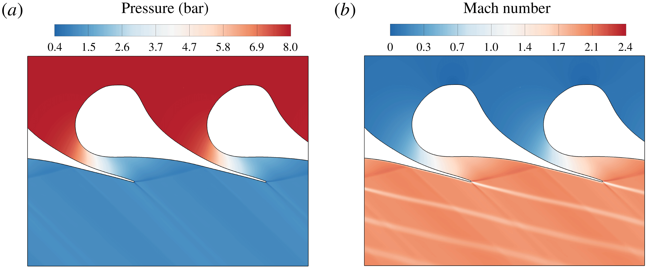
The typical flow field related to the expansion through the first stator of an ORC system is shown in figure 1. The blade is characterized by a large leading-edge region that acts as a converging section upstream of the section with minimum cross-sectional area (throat) and a diverging section downstream of the throat. The curved shape of the rear suction side imposes on the flow a significant unguided turning. The expansion corresponding to this turning process results in a severe over-speed, which ultimately generates a compression wave on the rear suction side of the blade, where the fish-tail shock originated at the trailing edge of the adjacent blade impinges. The two compression waves coalesce in a single strong shock at almost half axial chord downstream of the trailing edge, generating a strong azimuthal pressure gradient, which results in a massive entropy production.
Pressure field (a) and Mach number field (b) for the expansion of fluid MM in a representative turbine cascade. The upstream total pressure and temperature are
 $P_{0}^{t}=8.0~\text{bar}$
,
 $T_{0}^{t}=270\,^{\circ }\text{C}$
, respectively. The outlet static pressure is
 $P_{1}=1.1\,\text{bar}$
. Details on the numerical simulation in § 3.1.

Several studies (Schuster, Karellas & Aumann Reference Schuster, Karellas and Aumann2010; Lai, Wendland & Fischer Reference Lai, Wendland and Fischer2011) indicate that a potential gain in efficiency may be achieved by employing high-temperature ORCs, in particular supercritical cycles. Within this framework, the occurrence of non-ideal effects cannot be excluded. An example can be found in the work of Colonna et al. (Reference Colonna, Harinck, Rebay and Guardone2008), where some numerical simulations display a non-monotonic Mach number in the blade channel. This result, however, was not commented in light of its potential influence on the aerodynamic performance of the cascade. Whether non-ideal effects in the expansion process can affect the turbine performance and design is still unclear.
The present study contributes to the understanding of non-ideal flows evolving in supersonic nozzle cascades, by showing the role of non-ideal effects in the turbine performance and discussing their design implications. To this end, exemplary flows of siloxane MM (hexamethyldisiloxane,
 $\text{C}_{6}\text{H}_{18}\text{OSi}_{2}$
) in nozzle cascades are considered and compared. MM is a molecularly complex fluid currently employed in ORC power plants (Colonna et al.
Reference Colonna, Casati, Trapp, Mathijssen, Larjola, Turunen-Saaresti and Uusitalo2015) and is chosen here as representative of the class of fluids where non-ideal effects can be observed. In fact, several studies (Cramer & Best Reference Cramer and Best1991; Cramer & Crickenberger Reference Cramer and Crickenberger1992; Guardone & Vimercati Reference Guardone and Vimercati2016; Vimercati et al.
Reference Vimercati, Gori and Guardone2018) indicate that qualitatively similar behaviour is expected between different fluids exhibiting
 $0<\unicode[STIX]{x1D6E4}<1$
. Therefore, although conducted on a specific fluid, the present analysis is arguably of more general validity and thus its outcomes may be extended to other fluids relevant to the ORC field.
In the cases analysed here, the nozzle operates in the non-ideal gas-dynamic regime. However, depending on the upstream total conditions, two very different operating regimes can establish: one mirrors the ideal-gas scenario and is obtained with relatively dilute conditions at the cascade inlet; the other one, obtained for high-pressure inlet conditions, is characterized by non-ideal effects. For both operating regimes, a parametric study, in which the boundary conditions of the turbine cascade are changed, is performed from the perspective of assessing the off-design behaviour.
The structure of this work is as follows. Section 2 recalls the theoretical foundation of non-ideal compressible-fluid dynamics. The departure from ideal-gas behaviour is examined with reference to the basic flow phenomena involved in the turbine expansion. In § 3, numerical simulations of nozzle cascades are presented. The flow solver is described in § 3.1. The blade configurations and operating conditions used for the numerical investigation are illustrated in § 3.2 and a dedicated grid assessment is performed in § 3.3. The core of the present manuscript is the parametric study presented in §§ 3.4 and 3.5 for each operating regime occurring in the nozzle cascade. Finally, § 4 provides the concluding remarks.
2 Non-ideal effects in expanding flows
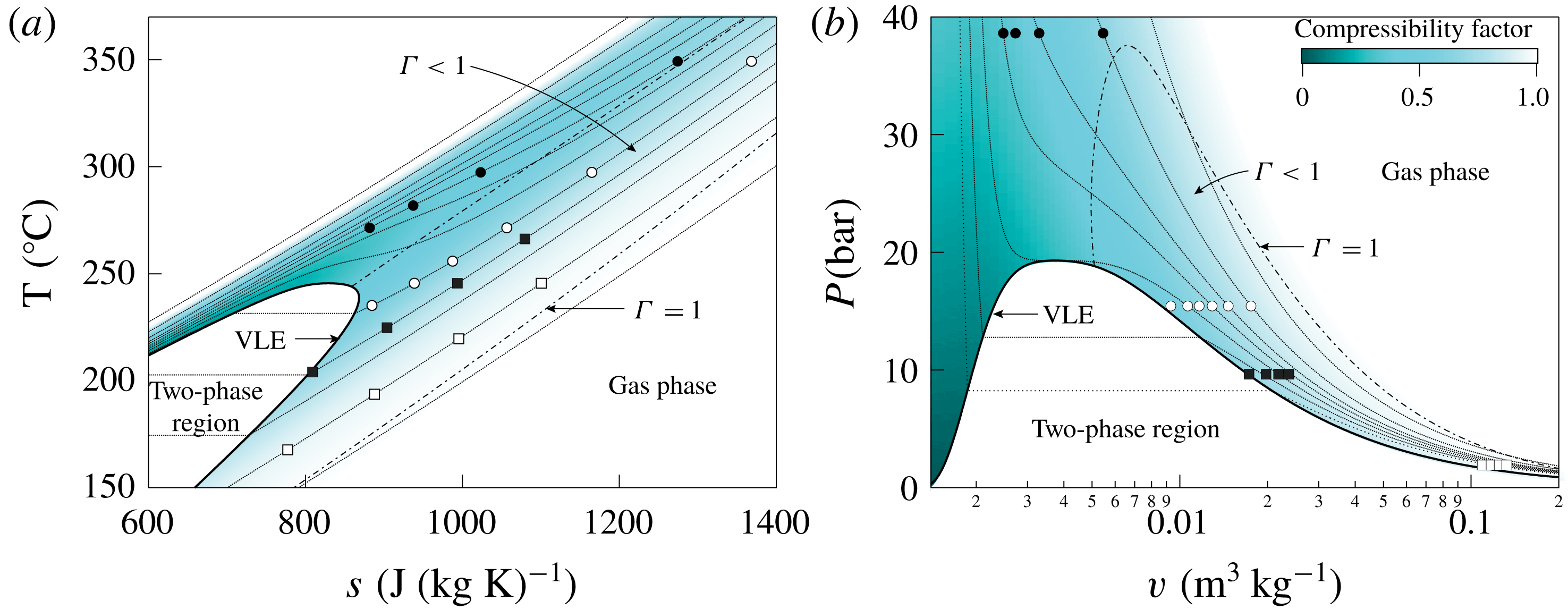
The onset of anomalous compressibility-related effects for flow variables close to the corresponding critical values is anticipated and explained here by recalling available theoretical results. Specifically, well-known results from the theories of quasi-one-dimensional flows and oblique waves (Prandtl–Meyer waves and oblique shock waves) are briefly reported to demonstrate the relevant qualitative and quantitative differences that emerge when the flow evolution occurs in the non-ideal gas-dynamic regime, rather than in dilute-gas conditions. The fluid considered hereafter, namely the siloxane MM, is modelled using the state-of-the-art multi-parameter equation of state formulated by Thol et al. (Reference Thol, Dubberke, Rutkai, Windmann, Köster, Span and Vrabec2016), see appendix A. The states selected for the theoretical studies of this section are reported in the well-known
 $T$
–
 $s$
(temperature–entropy) and
 $P$
–
 $v$
(pressure–specific volume) diagrams of figure 2.
Thermodynamic diagrams for MM showing the states used in the parametric studies: ▪ total conditions for isentropic nozzle flows in figures 3(a) and 4(a); ● total conditions for isentropic nozzle flows in figures 3(b) and 4(b); ▫ upstream thermodynamic state for Prandtl–Meyer waves of figure 5(a) and for oblique shock waves of figure 6(a); ○ upstream thermodynamic state for Prandtl–Meyer waves of figure 5(b) and for oblique shock waves of figure 6(b). A map of the compressibility factor
 $z=Pv/RT$
, where
 $R$
is the specific gas constant, is superposed. Dotted lines
 $(\cdots \,)$
represent isobars (a) or isotherms (b); dash-dotted lines (
 $\cdot -\cdot$
) identify
 $\unicode[STIX]{x1D6E4}=1$
.
Firstly, steady quasi-one-dimensional flow (Thompson Reference Thompson1988) is used as representative of the expansion process through a variable-area duct (inviscid and with constant total enthalpy
 $h^{t}=h+u^{2}/2$
, where
 $h$
is the specific enthalpy and
 $u$
the fluid velocity). Figure 3 shows the distribution of the Mach number
 $M=u/c$
with the pressure, for different total conditions chosen along the same isobaric line, which is
 $P^{t}=0.5\,P_{c}$
in figure 3(a) and
 $P^{t}=2\,P_{c}$
in figure 3(b), where
 $P^{t}$
is the total pressure (i.e. the pressure in stagnation condition) and
 $P_{c}$
is the critical pressure.
Despite
 $\unicode[STIX]{x1D6E4}<1$
at the selected total states, at relatively low total pressures and high temperatures (figure 3
a), most of the expansion occurs in dilute-gas conditions. Thus, the distributions of the Mach number are qualitatively identical and also quantitatively very similar to that computed from the ideal-gas model, which depends on the pressure ratio
 $P^{t}/P$
only. The ideal-gas limit curves hereafter are all obtained by setting
 $\unicode[STIX]{x1D6FE}=c_{p,\infty }(T_{c})/c_{v,\infty }(T_{c})$
, where
 $c_{p,\infty }$
and
 $c_{v,\infty }$
are the specific heats in the ideal-gas limit and
 $T_{c}$
is the critical temperature. In the present case,
 $\unicode[STIX]{x1D6FE}=1.026$
.
The effects of the non-ideal thermodynamic behaviour of the fluid can be fully appreciated by selecting thermodynamic states in the proximity of the critical point or in the supercritical region. The scenario observed in figure 3(b) is representative of the flow evolution in the non-ideal gas-dynamic regime and involves not only a marked quantitative difference with respect to its ideal-gas counterpart, but also important qualitative differences. Indeed, extrema in the Mach number may possibly occur, see for example case
 $T^{t}=1.05\,T_{c}$
in figure 3(b), where
 $T^{t}$
is the total temperature. As a result, the Mach number is no longer monotonic along the isentropic expansion. This follows immediately from the analysis of Cramer & Best (Reference Cramer and Best1991), in which the parameter
 $$\begin{eqnarray}J=1-\unicode[STIX]{x1D6E4}-\frac{1}{M^{2}}=\frac{\unicode[STIX]{x1D70C}}{M}\frac{\text{d}M}{\text{d}\unicode[STIX]{x1D70C}}\end{eqnarray}$$
is introduced as a non-dimensional measure of the Mach number derivative with the density (or pressure, after straightforward manipulation) and condition
 $J>0$
is recognized as the necessary condition for the Mach number to decrease along isentropic expansions.
Mach number distribution for quasi-one-dimensional flow of fluid MM with total pressure (a)
 $P^{t}=0.5\,P_{c}$
and (b)
 $P^{t}=2\,P_{c}$
; each solid line corresponds to a different value of the total temperature
 $T^{t}$
, while dotted lines are obtained from the ideal-gas model of MM.
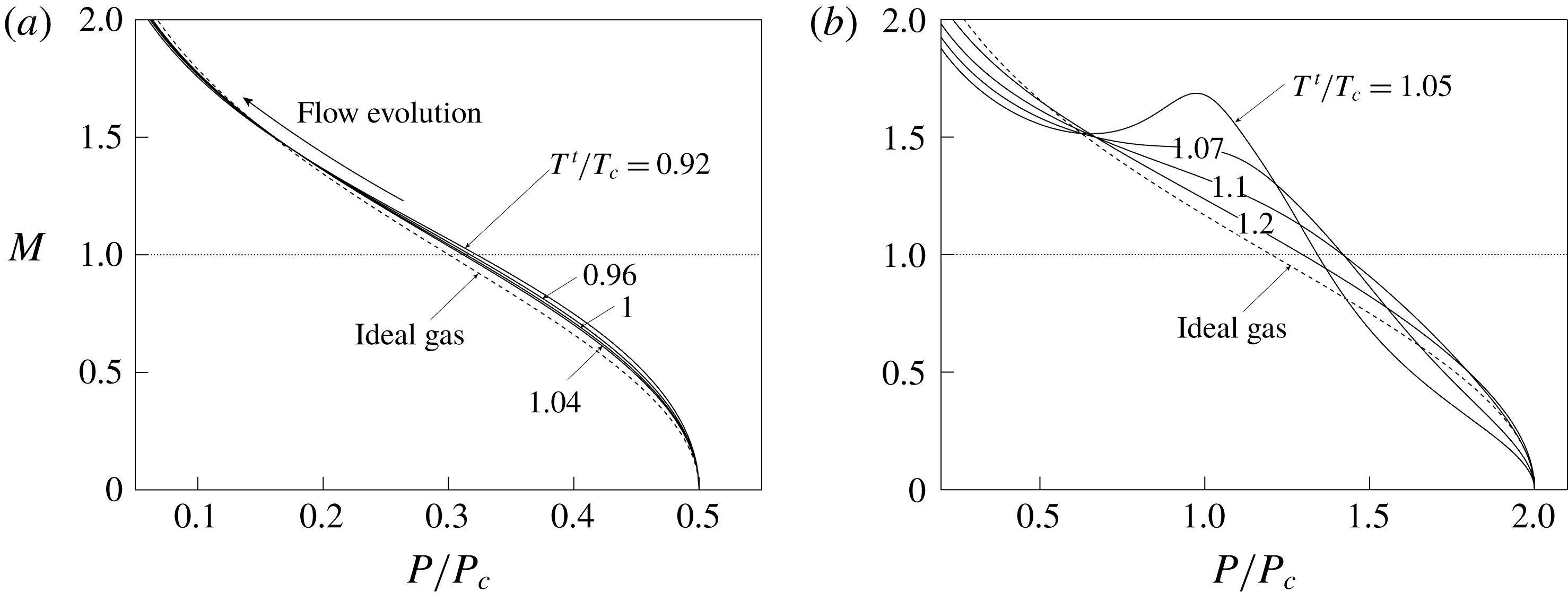
Figure 4 reports the distribution of the area ratio
 $A/A^{\ast }$
with the pressure, where
 $A^{\ast }$
is the critical area (at which
 $M=1$
), for different total conditions chosen along the same isobaric lines as above, namely
 $P^{t}=0.5\,P_{c}$
in figure 4(a) and
 $P^{t}=2P_{c}$
in figure 4(b). In both cases, the distribution of the area ratio is qualitatively similar to that of the ideal-gas limit. However, significant quantitative differences can be appreciated in the exemplary non-ideal case depicted in figure 4(b). As an example, expansion from total conditions up to
 $A/A^{\ast }=2$
corresponds to an expansion ratio
 $\unicode[STIX]{x1D6FD}=P^{t}/P=2.76$
from
 $T^{t}=1.05\,T_{c}$
and to
 $\unicode[STIX]{x1D6FD}=6.78$
in the ideal-gas limit (
 $T^{t}\rightarrow \infty$
at fixed
 $P^{t}$
). This should be compared to the case
 $P^{t}=0.5\,P_{c}$
, for which the same area ratio
 $A/A^{\ast }=2$
corresponds to
 $\unicode[STIX]{x1D6FD}=6.15$
from
 $T^{t}=1.05\,T_{c}$
. An alternative interpretation is connected with the design of the diverging portion of a nozzle aimed at realizing a given exit pressure ratio. The same exit pressure ratio is attained with a considerably larger exit-to-throat area ratio if expanding from high total-pressure conditions, thus involving severe non-ideal gas-dynamic effects.
Area ratio distribution for quasi-one-dimensional flow of fluid MM with total pressure (a)
 $P^{t}=0.5\,P_{c}$
and (b)
 $P^{t}=2\,P_{c}$
; each solid line corresponds to a different value of the total temperature
 $T^{t}$
, while dotted lines are obtained from the ideal-gas model of MM.

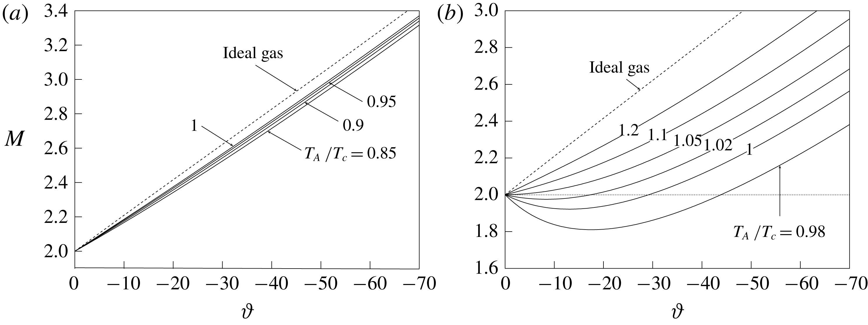
Next, oblique waves are examined, as representative of the turning processes of a supersonic stream that can possibly occur at the trailing edge of the turbine blades and in the rear blade section. Figure 5(a) reports the downstream Mach number against the flow deflection angle
 $\unicode[STIX]{x1D717}$
across Prandtl–Meyer waves, computed for a fixed upstream pressure
 $P_{A}=0.1\,P_{c}$
and Mach number
 $M_{A}=2$
, and different values of the upstream temperature
 $T_{A}$
. Each curve is computed using the definition of the Prandtl–Meyer function given by Cramer & Crickenberger (Reference Cramer and Crickenberger1992) and valid for arbitrary equations of state. At the selected upstream states,
 $\unicode[STIX]{x1D6E4}_{A}=0.96{-}0.98$
. In this range, the level of non-ideality is low enough that the actual features of Prandtl–Meyer waves are qualitatively similar to those computed from the ideal-gas model, despite a slight quantitative difference is still observed. Note, also, that across centred Prandtl–Meyer fans the fluid is isentropically expanded and therefore driven towards more dilute thermodynamic conditions. The non-ideal turning of a supersonic stream across Prandtl–Meyer waves is depicted in figure 5(b), which is obtained by setting the state upstream of the wave to
 $P_{A}=0.8\,P_{c}$
and
 $M_{A}=2$
, while different values of
 $T_{A}$
are considered. Remarkable quantitative and qualitative differences can be observed, most importantly the possibility that the Mach number decreases across the rarefaction wave, which is in contrast with the ideal-gas behaviour. For later convenience, Prandtl–Meyer waves featuring a decrease of the Mach number are referred to as non-ideal Prandtl–Meyer waves. The non-monotonic variation of the Mach number within the wave stems from thermodynamic states satisfying
 $J>0$
during the expansion (Cramer & Crickenberger Reference Cramer and Crickenberger1992). Indeed, the flow field corresponding to Prandtl–Meyer waves is isentropic and with constant total enthalpy, so that the same considerations of the one-dimensional case apply (Wheeler & Ong Reference Wheeler and Ong2013; Galiana, Wheeler & Ong Reference Galiana, Wheeler and Ong2016).
Variation of the Mach number with the wave deflection angle across Prandtl–Meyer waves in fluid MM with upstream Mach number
 $M_{A}=2$
and pressure (a)
 $P_{A}=0.1\,P_{c}$
and (b)
 $P_{A}=0.8\,P_{c}$
; each solid line corresponds to a different value of the total temperature
 $T_{A}$
, while dotted lines are obtained from the ideal-gas model of MM.
Finally, an analogous study is performed for oblique shock waves, see figure 6. Figures 6(a) and 6(b) are generated using the same upstream states of figures 5(a) and 5(b), respectively. Although the compression across the shock brings the flow towards more dense and therefore non-ideal thermodynamic conditions, at relatively low upstream pressures such as in figure 6(a), non-ideal effects are in fact not observed, except at the quantitative level and to a limited extent. On the contrary, in figure 6(b) we can observe a non-ideal discontinuous increase of the Mach number across oblique shocks. This phenomenon is the compression counterpart of the decrease of the Mach number in Prandtl–Meyer waves depicted in figure 5(b). Following Gori et al. (Reference Gori, Vimercati and Guardone2017) and Vimercati et al. (Reference Vimercati, Gori and Guardone2018), oblique shocks producing an increase of the Mach number will be referred to as non-ideal oblique shocks afterwards. It was demonstrated by Vimercati et al. (Reference Vimercati, Gori and Guardone2018) that weak oblique shocks from upstream states featuring
 $J_{A}>0$
are necessarily non-ideal oblique shocks. Moreover, due to non-isentropic effects, non-ideal oblique shocks can possibly occur from upstream states
 $J_{A}<0$
, although it is still required that
 $J>0$
along the shock adiabat connecting the upstream and downstream states.
Variation of the Mach number with the wave deflection angle across oblique shock waves in fluid MM with upstream Mach number
 $M_{A}=2$
and pressure (a)
 $P_{A}=0.1\,P_{c}$
and (b)
 $P_{A}=0.8\,P_{c}$
; each solid line corresponds to a different value of the total temperature
 $T_{A}$
, while dotted lines are obtained from the ideal-gas model of MM.

3 Gas dynamics of nozzle cascades in the non-ideal regime
In this section, the flow field within a linear nozzle cascade operating in the non-ideal gas-dynamic regime is examined by means of numerical simulations. While previous discussion focused on non-ideal effects in the inviscid limit, the correct modelling of the flow through the cascade should account for viscous effects (e.g. boundary layers). In this regard, a comparison between viscous and inviscid losses for the same class of turbine blades was presented by Pini et al. (Reference Pini, Persico, Pasquale and Rebay2015a ). This study shows the large impact of thermoviscous effects on the shock-wave formation and on the mixing process downstream of the cascade, pointing to the need of performing a viscous computation to predict such losses in a turbine cascade. To this end, Reynolds-averaged Navier–Stokes simulations are carried out.
The computational flow solver is described in § 3.1. The blade configurations used in this study are presented in § 3.2 and the grid-convergence assessment in § 3.3. Expansion through states featuring
 $\unicode[STIX]{x1D6E4}<1$
can possibly present very different behaviours, according to the occurrence of diverse non-ideal effects. Three exemplary operating conditions (each consisting of a design point and selected off-design cases) are presented in §§ 3.4 and 3.5 to illustrate the larger variability and diversity of the flow evolution offered by the non-ideal thermodynamics.
3.1 Computational flow model
Numerical simulations are carried out with ANSYS-CFX 18.1®. No-slip and adiabatic conditions are imposed on the blade surface. Axial flow is prescribed at the inlet along with total pressure and temperature (
 $P_{0}^{t}$
,
 $T_{0}^{t}$
). At the outlet, an average static pressure
 $P_{1}$
is imposed; local pressure differences of
 $5\,\%$
are allowed. The outlet domain is placed at 8 axial chords downstream of the trailing edge to avoid spurious pressure wave reflections. Since only blade-to-blade effects are of interest, quasi-three-dimensional simulations are carried out by considering a straight streamtube around the midspan (free-slip conditions at the end walls). A single-blade passage is considered by exploiting periodic boundary conditions. The employed turbulence model is
 $k{-}\unicode[STIX]{x1D714}$
SST, whose boundary conditions are set as turbulence intensity (
 $TI=5\,\%$
for all simulations) and eddy viscosity ratio (
 $\unicode[STIX]{x1D707}_{t}/\unicode[STIX]{x1D707}=10$
for all simulations). Note that these boundary conditions have very limited influence on the cascade performance for moderate values of the upstream total pressure (
 $P_{0}^{t}$
up to
 $0.6P_{c}$
), see Romei, Congedo & Persico (Reference Romei, Congedo and Persico2019); we expected that the same considerations hold for a larger range of total pressures. The cascade Reynolds number, based on the blade chord and computed using the mass-flow-averaged density, dynamic viscosity and velocity, is
 $Re\simeq 2\times 10^{6}{-}10^{7}$
for the simulations involving an expansion far from the thermodynamic critical point. For the simulations close to the critical point, the comparatively larger thermodynamic variations result in a significant variation of the Reynolds number through the blade passage, from
 $Re\simeq 5\times 10^{6}$
(based on inlet quantities) to
 $Re\simeq 10^{8}$
(outlet quantities). Therefore, the cascade Reynolds number is large enough to assume fully turbulent boundary layer along the entire blade.
The turbulent Prandtl number is set to
 $Pr_{t}=1$
in all simulations, consistently with other studies (e.g. Otero Rodriguez et al.
Reference Otero Rodriguez, Patel, Diez Sanhueza and Pecnik2018). With reference to the peculiar dependence of thermodynamic properties on the temperature in the non-ideal gas-dynamic regime, it is still unclear whether a specific choice of the turbulent Prandtl number impacts the flow field and consequently the aerodynamic performance of the cascade. A sensitivity analysis on
 $Pr_{t}$
, in the range
 $Pr_{t}=0.1{-}1.5$
, was conducted and reveals negligible influence of this parameter on the flow fields (e.g. a maximum temperature variation of
 $0.05\,\%$
downstream of the cascade).
The thermodynamic model (multi-parameter equation of state of MM by Thol et al. Reference Thol, Dubberke, Rutkai, Windmann, Köster, Span and Vrabec2016, see also appendix A) is implemented using a look-up-table approach, which allows us to speed up the evaluation of the thermodynamic properties (see, e.g., Pini et al. Reference Pini, Spinelli, Persico and Rebay2015b ). Thermodynamic tables are built by referring to the NIST REFPROP® database (Lemmon, Huber & McLinden Reference Lemmon, Huber and McLinden2013), which also provides dedicated correlations for transport properties (Meier, Laesecke & Kabelac Reference Meier, Laesecke and Kabelac2004; Perkins et al. Reference Perkins, Sengers, Abdulagatov and Huber2013). High-resolution total variation diminishing (TVD) schemes (Barth & Jespersen Reference Barth and Jespersen1989) are employed in the discretization of both flow and turbulence equations. A central difference scheme is instead adopted for the diffusive flux. The suitability of the present computational set-up for simulations of non-ideal compressible flows near to the saturation curve and critical point is discussed and confirmed in the study of Pini et al. (Reference Pini, Vitale, Colonna, Gori, Guardone, Economon, Alonso and Palacios2017).
Computations are performed on structured hexahedral meshes. A proper cell clustering near blade walls is imposed to ensure
 $y^{+}\lesssim 1$
, thus avoiding the introduction of wall functions in the solution.
3.2 Blade configuration and operating conditions
The turbine cascades used in the following study result from an optimization procedure applied to the baseline cascade shown in figure 1. The baseline blade geometry was initially conceived for a combined heat and power application, featuring MDM (octamethyltrisiloxane,
 $\text{C}_{8}\text{H}_{24}\text{O}_{2}\text{Si}_{3}$
) as working fluid (Colonna et al.
Reference Colonna, Harinck, Rebay and Guardone2008). Shape-optimization procedures proved to be successful in reducing the losses (in particular, shock losses) and improving the cascade performance (see, e.g., Vitale et al.
Reference Vitale, Albring, Pini, Gauger and Colonna2017).
The optimization procedure used in the present work exploits a surrogate-based evolutionary strategy, detailed in Persico, Rodriguez-Fernandez & Romei (Reference Persico, Rodriguez-Fernandez and Romei2019). The baseline cascade is parametrized with a single B-spline curve, whose shape and smoothness are controlled by a non-uniform control-point distribution. The trailing edge is modelled as a circular arc tangent to the B-spline curve in one of its extremity and it can be moved only rigidly (no variation of trailing-edge shape or thickness is allowed). The control-point locations are the design variables to be optimized; only control points in the divergent part of the blade are considered in the optimization set-up. The cascade entropy production, namely the difference between the mass-flow-averaged entropy between the mixed-out section (4 axial chords downstream of the cascade trailing edge) and the inlet, is the objective function of the present optimization problem. It is computed with the same flow solver discussed in § 3.1, using a 100k-cell mesh in the blade-to-blade plane to speed up the computation. The latter choice is motived by the fact that even the coarsest mesh discussed in the grid-convergence assessment (see § 3.3 below) exhibits negligible variations in the overall cascade-loss estimation. A space-filling technique is first used to explore the design space. An initial response surface based on a Gaussian process is then determined based on these evaluations. The actual performance of the surface-response global minimum, found via genetic algorithms, is evaluated and the new value is added to the previous design pools. A new surface response is generated and the procedure is iteratively repeated to increase the reliability of the surrogate prediction close to the expected global minimum. The process is stopped when the difference between the surrogate estimation and the actual value, i.e. the value provided by the flow solver, is below a given threshold for several iterations.
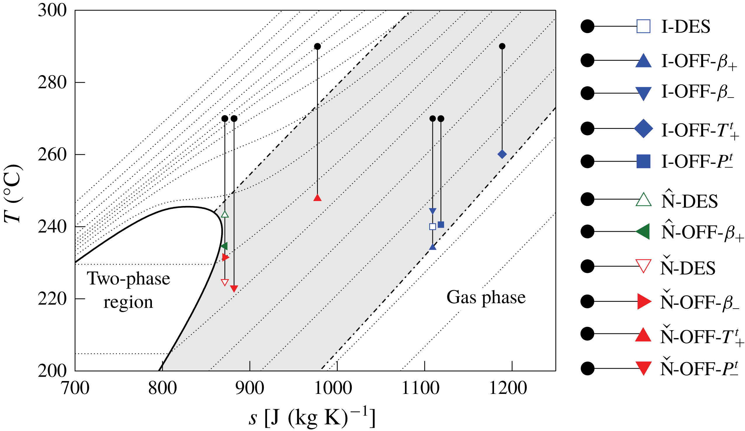
Temperature versus specific entropy diagram for MM, showing the expansion processes considered in the present work. Dotted lines
 $(\cdots \,)$
represent different isobars. Dash-dotted lines (
 $\cdot -\cdot$
) identify
 $\unicode[STIX]{x1D6E4}=1$
.
Boundary conditions for numerical simulations;
 $P_{0}^{t}$
and
 $T_{0}^{t}$
are the total upstream pressure and the total upstream temperature, respectively,
 $P_{1}$
is the downstream static pressure and
 $\unicode[STIX]{x1D6FD}=P_{0}^{t}/P_{1}$
.

The optimization is performed for three exemplary design conditions, namely
 $\text{I}\text{-}\text{DES}$
,
 $\hat{\text{N}}\text{-}\text{DES}$
and
 $\check{\text{N}}\text{-}\text{DES}$
, reported in table 1 and depicted in the
 $T$
–
 $s$
diagram in figure 7. The design case labelled
 $\text{I}\text{-}\text{DES}$
recalls the same application, in terms of inlet and outlet thermodynamic conditions of the nozzle cascade, examined by Colonna et al. (Reference Colonna, Harinck, Rebay and Guardone2008), but using MM as working fluid. For thermodynamic conditions, the flow evolution is similar to that of an ideal gas, thus the expansion inside the nozzle depends almost only on the expansion ratio and on the ratio between specific heats. On this basis,
 $\text{I}\text{-}\text{DES}$
and related off-design conditions
 $\text{I}\text{-}\text{OFF}$
-
 $i$
,
 $i=\{\unicode[STIX]{x1D6FD}_{+},\unicode[STIX]{x1D6FD}_{-},T_{+}^{t},P_{-}^{t}\}$
, are referred to as the ideal-like operating regime of the nozzle cascade.
Operating conditions
 $\hat{\text{N}}\text{-}\text{DES}$
and
 $\check{\text{N}}\text{-}\text{DES}$
are chosen to highlight non-ideal effects on the flow features arising in the proximity of the blade trailing edge, which are highly influential on the overall cascade performances. Two peculiar operating conditions can be identified in which the Mach number at the trailing edge is close to a local maximum (
 $\hat{\text{N}}\text{-}\text{DES}$
) or to a local minimum (
 $\check{\text{N}}\text{-}\text{DES}$
). For convenience, these operating conditions along with the related off-design cases
 $\hat{\text{N}}\text{-}\text{OFF}\text{-}\unicode[STIX]{x1D6FD}_{+}$
and
 $\check{\text{N}}\text{-}\text{OFF}$
-
 $i$
,
 $i=\{\unicode[STIX]{x1D6FD}_{-},T_{+}^{t},P_{-}^{t}\}$
, are referred to, in the following, as the non-ideal operating regime of the nozzle cascade.
The blades optimized for
 $\text{I}\text{-}\text{DES}$
,
 $\hat{\text{N}}\text{-}\text{DES}$
and
 $\check{\text{N}}\text{-}\text{DES}$
are shown in figure 8. All optimal blades feature a higher curvature in the diverging channel and an almost straight profile in the rear part of the blade. In this way, the main compression shock wave is almost eliminated, adapting the nozzle-cascade geometry to the expansion process on which the optimization is performed. In the non-ideal gas-dynamic regime, relatively small expansion ratios can produce large outlet Mach numbers, due to the low values of the speed of sound. As an example, operating condition
 $\hat{\text{N}}\text{-}\text{DES}$
features
 $M\approx 1.8$
at the nozzle exit with
 $\unicode[STIX]{x1D6FD}=2.2$
. Thus, converging–diverging shapes are mandatory to cope with the supersonic expansion. The resulting geometries are consistent with the quasi-one-dimensional theory. The selected design conditions are such that
 $A_{e}/A^{\ast }=2.2$
for
 $\text{I}\text{-}\text{DES}$
,
 $A_{e}/A^{\ast }=1.4$
for
 $\hat{\text{N}}\text{-}\text{DES}$
and
 $A_{e}/A^{\ast }=2.2$
for
 $\check{\text{N}}\text{-}\text{DES}$
, where
 $A_{e}$
is the equivalent-nozzle exit area. Note that the optimized blades for
 $\text{I}\text{-}\text{DES}$
and
 $\check{\text{N}}\text{-}\text{DES}$
are very similar, despite the significantly different expansion ratios. On the other hand, the optimal blade for
 $\hat{\text{N}}\text{-}\text{DES}$
differs significantly from all the others due to the much smaller exit-to-throat area ratio.
Optimized nozzle cascades for
 $\text{I}\text{-}\text{DES}$
(——, blue),
 $\hat{\text{N}}\text{-}\text{DES}$
(——, green) and
 $\check{\text{N}}\text{-}\text{DES}$
(——, red). The optimization is aimed at minimizing the entropy production.

3.3 Grid assessment and near-wall resolution
Mesh sensitivity analysis is carried out on four different grid refinements, consisting of approximately 100k, 200k, 400k, 600k cells in the blade-to-blade plane (single-blade passage). Grid convergence is assessed on operating condition
 $\check{\text{N}}\text{-}\text{DES}$
, detailed in § 3.2, which involves the highest Reynolds numbers and the strongest non-ideal effects among the other cases.
Figure 9(a) shows the density distribution along a reference plane located at half axial chord downstream of the cascade, for the different levels of refinements. Grid convergence is achieved starting from the 400k-cell mesh. Other thermodynamic quantities such as pressure, temperature, entropy and speed of sound show trends very similar to that of figure 9(a). The same is observed for the velocity and Mach number distributions.
In figure 9(b), the turbulent kinetic energy profiles are plotted. Higher deviations, with respect to mean-flow quantities, are observed between the different grids. It should also be noticed that the turbulence fields may not achieve a grid-independent state in the presence of shock waves (Sinha, Mahesh & Candler Reference Sinha, Mahesh and Candler2003). Nevertheless, the 400k-cell and 600k-cell meshes show comparable values of the peak and average turbulent kinetic energy. The distribution of the turbulent kinetic energy is relevant for the prediction of the mixing process downstream of the blades and its evaluation is indeed critical if the stator–rotor axial gap is very small. However, in the present study we are concerned with the performance of the stator alone, thus mixed-flow conditions downstream of the cascade are always achieved by virtue of the wide fluid domain employed in all simulations (see § 3.1). Similar considerations apply to the turbulence frequency distribution on the different grids. Thus, the 400k-cell mesh, illustrated in figure 9(c), is chosen as the most suitable for the purpose of the present investigation. The simulations of operating conditions different from the
 $\check{\text{N}}\text{-}\text{DES}$
are performed on grids with similar topology and refinement.
Grid-convergence assessment on
 $\check{\text{N}}\text{-}\text{DES}$
: azimuthal distributions of (a) density and (b) turbulent kinetic energy evaluated on a reference plane located at half axial chord downstream of the cascade; (c) details of the 400k-cell mesh (convergence achieved). The cell count refers to the single-blade passage.

The kinetic energy loss coefficient
 $\unicode[STIX]{x1D701}_{S}$
,
 $$\begin{eqnarray}\unicode[STIX]{x1D701}_{S}=\frac{h_{mix}-h_{mix,is}}{u_{mix}^{2}/2},\end{eqnarray}$$
where
 $h_{mix}$
,
 $h_{mix,is}$
and
 $u_{mix}^{2}/2$
are the mass-flow-averaged specific enthalpy, isentropic specific enthalpy and kinetic energy, respectively, evaluated at the mixed-out section, is used to evaluate the cascade performance. This coefficient accounts for all loss sources such as shock (and related shock–boundary layer interaction), mixing and viscous losses, thus giving an overall indication of the cascade performance. It is found that the maximum difference with respect to the finest-grid value (
 $\unicode[STIX]{x1D701}_{S}=3.6\,\%$
) is
 $0.3\,\%$
(100k-cell grid).
Velocity profiles in wall units (a) in proximity of the channel throat and (b) in the rear part of the suction side, downstream of the point of shock reflection. Markers denote the computed
 $u^{+}$
values at grid nodes; solid lines correspond to
 $u^{+}=y^{+}$
and to the log law
 $u^{+}=2.5\ln y^{+}+5.5$
.

In the above grid assessment, the near-wall grid resolution has been kept constant among the various levels of refinement. Velocity profiles in the boundary layer at selected locations are shown in figure 10, specifically in proximity of the throat and in the rear part of the blade suction side, downstream of the point where the fish-tail shock is reflected. The distributions shown in this figure are computed using the 400k-cell mesh. The computed velocity profiles are qualitatively similar to each other, consistently with the fact that there is no shock-induced boundary layer separation. Relatively small deviations are observed with respect to the incompressible, zero-pressure-gradient laws for the viscous sublayer and logarithmic region. This is not surprising in fluids having large heat capacities, due to the very small values of the Eckert number (see Kluwick Reference Kluwick2004; Cinnella & Congedo Reference Cinnella and Congedo2007; Sciacovelli, Cinnella & Gloerfelt Reference Sciacovelli, Cinnella and Gloerfelt2017). Moreover, the computed temperature and density distributions in the boundary layer are nearly constant. Analogous considerations apply to other operating conditions listed in table 1.
3.4 Ideal-like operating regime of nozzle cascades
In this section we establish the general framework for the analysis of flows in nozzle cascades by focusing on the ideal-like operating regime. Concepts familiar to ideal-gas flows in nozzle cascades are reviewed and extended to the non-ideal thermodynamic description of the flow. We consider the converging–diverging nozzle optimized for the design condition
 $\text{I}\text{-}\text{DES}$
. In addition to the design condition, cascade performances are also analysed by considering four different off-design expansions
 $\text{I}\text{-}\text{OFF}$
-
 $i$
,
 $i=\{\unicode[STIX]{x1D6FD}_{+},\unicode[STIX]{x1D6FD}_{-},T_{+}^{t},P_{-}^{t}\}$
. Each of these processes is detailed in table 1 and shown graphically in the
 $T$
–
 $s$
thermodynamic plane of figure 7. Note that total temperature values used throughout this work lie within the thermal stability limit of the working fluid (Preissinger & Bruggemann Reference Preissinger and Bruggemann2016; Keulen et al.
Reference Keulen, Gallarini, Landolina, Spinelli, Iora, Invernizzi, Lietti and Guardone2018).
Pressure and Mach number distributions for
 $\text{I}\text{-}\text{DES}$
are reported in figure 11. The optimization, performed in such conditions, generates a nozzle cascade which features a smooth expansion process, characterized by a nearly uniform-pressure field downstream of the cascade. A weak fish-tail shock stems from the trailing edge. Quantitatively, the nozzle cascade exhibits a kinetic energy loss coefficient
 $\unicode[STIX]{x1D701}_{S}=3.8\,\%$
. This value is used as reference to quantify the impact of off-design conditions on the blade performance within the ideal-like operating regime. Furthermore,
 $\text{I}\text{-}\text{DES}$
displays a mass-flow-averaged Mach number measured at half axial chord downstream of the trailing edge (representing a plausible stator–rotor gap) equal to
 $M_{05}=1.94$
.
Pressure field (a) and Mach number field (b) for
 $\text{I}\text{-}\text{DES}$
. The working fluid is MM.
The effect of variations in the outlet static pressure for the ideal-like operating regime: (a,b) pressure and Mach number fields for
 $\text{I}\text{-}\text{OFF}\text{-}\unicode[STIX]{x1D6FD}_{+}$
; (c,d) pressure and Mach number fields for
 $\text{I}\text{-}\text{OFF}\text{-}\unicode[STIX]{x1D6FD}_{-}$
; (e,f) pressure and Mach number distributions along a reference streamline, approximately following the centreline of the blade channel. The working fluid is MM.

Off-design cases
 $\text{I}\text{-}\text{OFF}\text{-}\unicode[STIX]{x1D6FD}_{+}$
and
 $\text{I}\text{-}\text{OFF}\text{-}\unicode[STIX]{x1D6FD}_{-}$
expand from the design superheated conditions to lower and higher outlet pressures, respectively, with respect to the design value. These conditions are very common in power systems due to the seasonal variation of ambient temperature, which directly affects the temperature of condensation and hence the turbine outlet pressure.
Case
 $\text{I}\text{-}\text{OFF}\text{-}\unicode[STIX]{x1D6FD}_{+}$
imposes on the flow an expansion characterized by a higher pressure ratio. In the present study, the increased pressure ratio is derived by imposing a decrease of
 $20\,^{\circ }\text{C}$
of the condensation temperature; the resulting change in the turbine pressure ratio was propagated to that of the first stator assuming that the turbine is composed by two stages and that the distribution of the enthalpy drops among each cascade remains unchanged. According to quasi-one-dimensional theory, in the blade channel the flow expands as in the design condition and a post-expansion is required to match the lower outlet pressure. This behaviour can be qualitatively recognized in figures 12(a,b) and 12(e,f). The main contribution to the post-expansion is given by the wider Prandtl–Meyer fan generated on the pressure side of the trailing edge. However, the cascade loss coefficient increases to
 $\unicode[STIX]{x1D701}_{S}=4.2\,\%$
due to the formation of a stronger shock wave on the opposite side of the trailing edge. For the selected upstream total conditions, the additional expansion provides a higher Mach number (
 $M_{05}=2.15$
) at the outlet.
The effect of a reduced pressure ratio is illustrated by case
 $\text{I}\text{-}\text{OFF}\text{-}\unicode[STIX]{x1D6FD}_{-}$
, shown in figure 12(c–f) and obtained by increasing the condensation temperature of
 $20\,^{\circ }\text{C}$
with the same approach used above for
 $\text{I}\text{-}\text{OFF}\text{-}\unicode[STIX]{x1D6FD}_{+}$
to compute the outlet pressure. The pressure distribution shown in figures 12(c) and 12(e) is strongly affected by the onset of a strong shock wave, especially where the fish-tail shock reflects. As a consequence, cascade losses increase showing a net increment of the kinetic energy loss coefficient to
 $7.7\,\%$
. Note that the entropy increase across the shocks is only a small share of the overall entropy production. In this regard, the analysis of the entropy fields reveals that (i) the entropy jump across shock waves is negligible if compared to the entropy increase generated in the boundary layer and in the mixing downstream of the cascade and (ii) the mixing losses increase with higher non-uniformities caused by stronger shocks in off-design operation (Persico et al.
Reference Persico, Rodriguez-Fernandez and Romei2019). Moreover, the rotor will experience a higher aerodynamic forcing induced by the presence of shock waves. Stronger shock waves lead to a reduction of the Mach number downstream of the nozzle cascade (
 $M_{05}=1.75$
), as expected in ideal-like conditions.
The effect of variations in the upstream total conditions for the ideal-like operating regime: (a,b) pressure and Mach number fields for
 $\text{I}\text{-}\text{OFF}\text{-}T_{+}^{t}$
; (c,d) pressure and Mach number fields for
 $\text{I}\text{-}\text{OFF}\text{-}P_{-}^{t}$
; (e,f) pressure and Mach number distributions along a reference streamline, approximately following the centreline of the blade channel. The working fluid is MM.

The following off-design cases
 $\text{I}\text{-}\text{OFF}\text{-}T_{+}^{t}$
and
 $\text{I}\text{-}\text{OFF}\text{-}P_{-}^{t}$
feature the design pressure ratio, but the fluid is expanded from different upstream total temperatures and pressures, respectively, with respect to
 $\text{I}\text{-}\text{DES}$
. These conditions are representative of part-load control strategies, for example in ORC power systems.
Case
 $\text{I}\text{-}\text{OFF}\text{-}T_{+}^{t}$
corresponds to an increase of the upstream total temperature. In this case, quasi-one-dimensional theory of ideal gases predicts no differences with respect to the design flow evolution, as the expansion process is governed only by the expansion ratio and the specific heats ratio, which remains fairly constant by increasing the inlet temperature of
 $20\,^{\circ }\text{C}$
. The flow-field distributions reported in figures 13(a,b) and 13(e,f) confirm qualitatively this behaviour, showing no appreciable differences with respect to the ones presented in figure 11 for the design condition. Quantitatively, both the outlet Mach number (
 $M_{05}=1.94$
) and the kinetic energy loss coefficient (
 $\unicode[STIX]{x1D701}_{S}=3.8\,\%$
) are very close to the design values.
Finally,
 $\text{I}\text{-}\text{OFF}\text{-}P_{-}^{t}$
features a lower upstream total pressure. The outlet pressure is also reduced to maintain the design pressure ratio. Similarly to
 $\text{I}\text{-}\text{DES}$
and
 $\text{I}\text{-}\text{OFF}\text{-}T_{+}^{t}$
, the same pressure ratio entails qualitatively similar flow fields, see figure 13(c–f), and in turn analogous values of the outlet Mach number (
 $M_{05}=1.94$
) and of the loss coefficient (
 $\unicode[STIX]{x1D701}_{S}=3.8\,\%$
).
To summarize, we have reported the performance of a supersonic converging–diverging cascade operating in the non-ideal gas-dynamic regime (
 $\unicode[STIX]{x1D6E4}<1$
) but qualitatively showing ideal-gas behaviour. In the ideal-like operating regime, four off-design conditions were analysed, drawing the following conclusions: (i) an increase of the pressure ratio delivers a larger outlet Mach number with a slight increase of cascade losses; (ii) reducing the pressure ratio, the nozzle cascade features significantly lower performance due to the onset of a strong shock wave to match the higher outlet pressure; (iii) variation of the upstream total state at the same pressure ratio has practically no effect on the cascade performance.
3.5 Non-ideal operating regime of nozzle cascades
In order to investigate the performance of the representative nozzle cascades working in the non-ideal operating regime, two different blades are considered, which are designed for expansions
 $\hat{\text{N}}\text{-}\text{DES}$
and
 $\check{\text{N}}\text{-}\text{DES}$
. Off-design behaviour is assessed on four cases labelled
 $\hat{\text{N}}\text{-}\text{OFF}\text{-}\unicode[STIX]{x1D6FD}_{+}$
and
 $\check{\text{N}}\text{-}\text{OFF}$
-
 $i$
,
 $i=\{\unicode[STIX]{x1D6FD}_{-},T_{+}^{t},P_{-}^{t}\}$
. Each of these cases is detailed in table 1 and the corresponding expansion processes are reported in the
 $T$
–
 $s$
thermodynamic plane of figure 7.
(a,b) Pressure and Mach number fields for
 $\hat{\text{N}}\text{-}\text{DES}$
; (c,d) pressure and Mach number fields for
 $\check{\text{N}}\text{-}\text{DES}$
; (e,f) pressure and Mach number distributions along a reference streamline, approximately following the centreline of the blade channel. The working fluid is MM.

The present choice of the upstream total state for both design conditions offers the possibility to observe and examine effects associated with the non-ideal evolution of the Mach number. According to quasi-one-dimensional theory, the isentropic expansion from
 $P_{0}^{t}=40\,\text{bar}$
and
 $T_{0}^{t}=270\,^{\circ }\text{C}$
features a non-monotonic Mach number (see figure 3
b) with a remarkable difference (
 $\unicode[STIX]{x0394}M\approx 0.26$
) between the two stationary points. Moreover, if
 $J>0$
in the neighbourhood of the trailing edge (i.e. the expansion through the blade channel end between the two extrema), non-ideal Prandtl–Meyer fans and oblique shocks might establish. This scenario is clarified using two specific examples in which the expansion through the blade channel ends near a stationary point of the Mach number (local maximum for
 $\hat{\text{N}}\text{-}\text{DES}$
and local minimum for
 $\check{\text{N}}\text{-}\text{DES}$
). Note that a possible advantage deriving from this situation is the enhanced uniformity of the Mach number distribution within the stator–rotor axial gap, due to the relatively low sensitivity of the Mach number to perturbations in the outlet pressure (
 $J\approx 0$
).
Pressure and Mach number distributions for
 $\hat{\text{N}}\text{-}\text{DES}$
and
 $\check{\text{N}}\text{-}\text{DES}$
are shown in figure 14(a–f). For both cases, a pattern of weak oblique waves occurs downstream of the trailing edge, evidenced in the pressure contours. Inspection of the Mach number fields reveals that no appreciable variation of the Mach number is observed across the oblique waves patterns, owing to very small values of
 $J$
. Quite distinct values of the outlet Mach number are observed, namely
 $M_{05}=1.77$
for
 $\hat{\text{N}}\text{-}\text{DES}$
and
 $M_{05}=1.51$
for
 $\check{\text{N}}\text{-}\text{DES}$
. As a matter of fact, the comparatively lower value observed in
 $\check{\text{N}}\text{-}\text{DES}$
, which features instead an increased pressure ratio, is a consequence of the fact that
 $J>0$
along the expansion (indeed the local maximum of the Mach number moves within the blade channel). Cascade performances, used in the following to assess the off-design behaviour, are very similar between the two design cases and amount to
 $\unicode[STIX]{x1D701}_{S}=3.8\,\%$
for
 $\hat{\text{N}}\text{-}\text{DES}$
and
 $\unicode[STIX]{x1D701}_{S}=3.6\,\%$
for
 $\check{\text{N}}\text{-}\text{DES}$
.
The effect of variations in the outlet static pressure for the non-ideal operating regime: (a,b) pressure and Mach number fields for
 $\hat{\text{N}}\text{-}\text{OFF}\text{-}\unicode[STIX]{x1D6FD}_{+}$
; (c,d) pressure and Mach number fields for
 $\check{\text{N}}\text{-}\text{OFF}\text{-}\unicode[STIX]{x1D6FD}_{-}$
; (e,f) pressure and Mach number distributions along a reference streamline, approximately following the centreline of the blade channel. The working fluid is MM.

Cases
 $\hat{\text{N}}\text{-}\text{OFF}\text{-}\unicode[STIX]{x1D6FD}_{+}$
and
 $\check{\text{N}}\text{-}\text{OFF}\text{-}\unicode[STIX]{x1D6FD}_{-}$
, analogously to
 $\text{I}\text{-}\text{OFF}\text{-}\unicode[STIX]{x1D6FD}_{+}$
and
 $\text{I}\text{-}\text{OFF}\text{-}\unicode[STIX]{x1D6FD}_{-}$
, respectively, aim at determining the impact of different pressure ratios on the cascade performance, likewise computed by decreasing/increasing the condensation temperature of
 $20\,^{\circ }\text{C}$
, with constant enthalpy drops across each single cascade. A five-stage turbine is assumed here to process the larger turbine pressure ratio, consistently with the latest trend in the ORC field (Bini & Colombo Reference Bini and Colombo2017). The upstream total conditions are instead kept constant. As the nomenclature suggests, the blades used in the off-design cases
 $\hat{\text{N}}\text{-}\text{OFF}\text{-}\unicode[STIX]{x1D6FD}_{+}$
and
 $\check{\text{N}}\text{-}\text{OFF}\text{-}\unicode[STIX]{x1D6FD}_{-}$
are those optimized for
 $\hat{\text{N}}\text{-}\text{DES}$
and
 $\check{\text{N}}\text{-}\text{DES}$
, respectively.
The larger pressure ratio in
 $\hat{\text{N}}\text{-}\text{OFF}\text{-}\unicode[STIX]{x1D6FD}_{+}$
is achieved by means of post-expansion, see figures 15(a,b) and 15(e,f). The actual features of the Mach number field downstream of the trailing edge differ significantly from those observed in the ideal-like operating regime. The Prandtl–Meyer fan generated on the pressure side of the trailing edge, and subsequently reflected on the suction side of the neighbouring blade, produces a non-ideal decrease of the Mach number. Past the trailing edge, the matching of pressure and flow direction across the wake is accomplished by a non-ideal oblique shock which increases the Mach number. Note that similar flow features can be observed also in
 $\hat{\text{N}}\text{-}\text{DES}$
, albeit to a much lower extent. The high amount of post-expansion of
 $\hat{\text{N}}\text{-}\text{OFF}\text{-}\unicode[STIX]{x1D6FD}_{+}$
can be further appreciated from the waviness of the wake. Overall, the prevailing effects is the Mach number decrease across the expansion waves downstream of the trailing edge, which ultimately results in
 $M_{05}=1.66$
(while
 $M_{05}=1.77$
in the design condition
 $\hat{\text{N}}\text{-}\text{DES}$
). The kinetic loss coefficient instead increases to
 $\unicode[STIX]{x1D701}_{S}=6.4\,\%$
, as expected, due to onset of the relatively strong shock generated at the trailing edge.
Configuration
 $\check{\text{N}}\text{-}\text{OFF}\text{-}\unicode[STIX]{x1D6FD}_{-}$
features a decreased pressure ratio. To accommodate the higher outlet pressure, a stronger oblique shock stems from the pressure side of the trailing edge and is reflected on the suction side of the neighbouring blade, whereas a rarefaction fan is generated on the opposite side of the trailing edge, as shown in figure 15(c–f). For both waves, a non-ideal variation of the Mach number is observed, namely the Mach number decreases across the Prandtl–Meyer expansion and increases across the oblique shock wave. The overall Mach number variation follows the non-ideal character of the compression process, resulting in
 $M_{05}=1.57$
(while
 $M_{05}=1.51$
in
 $\check{\text{N}}\text{-}\text{DES}$
). The stronger shock pattern in
 $\check{\text{N}}\text{-}\text{OFF}\text{-}\unicode[STIX]{x1D6FD}_{-}$
than in
 $\hat{\text{N}}\text{-}\text{OFF}\text{-}\unicode[STIX]{x1D6FD}_{+}$
is responsible for the comparatively larger increase of the loss coefficient (
 $\unicode[STIX]{x1D701}_{S}=7.5\,\%$
). The question arises as to whether the contribution of shock losses to the overall entropy production is influenced by non-ideal effects; inspection of the entropy fields shows that there is no substantial difference with respect to the ideal-like operating regime.
The situation depicted above for
 $\hat{\text{N}}\text{-}\text{OFF}\text{-}\unicode[STIX]{x1D6FD}_{+}$
and
 $\check{\text{N}}\text{-}\text{OFF}\text{-}\unicode[STIX]{x1D6FD}_{-}$
is opposed to the ideal-gas like scenario. The non-ideal variation of the outlet Mach number with the outlet pressure might have remarkable consequences on the operation of the entire turbine. As a matter of fact, the present supersonic cascades are prototypes of the first stators of ORC turbines. The nozzle is commonly followed by a transonic rotor, whose operational characteristics and performance are crucially dependent on the flow regime (whether subsonic or supersonic) associated with the relative flow at the inlet. The rotor-inlet flow is indeed proportional to the (absolute) Mach number at the outlet of the stator, modulated by the rotational speed. Supersonic relative flow at the rotor inlet are detrimental for the turbine flexibility and performance mainly due to the so-called unique-incidence phenomenon (Starken, Yongxing & Schreiber Reference Starken, Yongxing and Schreiber1984). Within this supersonic flow regime, the rotor leading edge behaves as a bluff body, enabling the formation of a bow shock upstream of the leading edge. Both the shock strength and its distance from the rotor leading edge are functions of the inlet relative Mach number and the leading-edge radius. Under this condition the inlet flow angle is no longer a free parameter but it is given by the bow–shock interaction among adjacent rotor cascades. It can be proved that, for a given rotor geometry, a unique pattern of characteristic lines is feasible, thus admitting a unique inlet flow angle (Starken Reference Starken1993). Therefore, the flow is chocked in the rotor cascade and it is not possible to adjust the mass flow by varying the upstream flow angle. Besides, supersonic rotor cascades may present a complex pattern of shock waves and shock–boundary layer interactions, which are likely to result in a lower stage efficiency as the Mach number at the rotor inlet increases (Rinaldi, Pecnik & Colonna Reference Rinaldi, Pecnik and Colonna2016). A proper design of the rotor cascade makes it possible to mitigate the aforementioned phenomena (see, e.g., Bufi & Cinnella Reference Bufi and Cinnella2018), even though such design is valid only for a specific operating condition. From this point of view, operating conditions similar to
 $\hat{\text{N}}\text{-}\text{DES}$
, i.e. tuned to obtain a local maximum of the Mach number near to the trailing edge, are advantageous against the unique incidence phenomenon. Indeed, both an increase and a decrease of the outlet pressure would reduce the outlet Mach number, thus increasing the safety margin for unique incidence. On the contrary, for design conditions analogous to
 $\check{\text{N}}\text{-}\text{DES}$
, a Mach number increase is expected for whatever pressure-ratio variation in the neighbourhood of the design point. In particular, a non-ideal effect that unexpectedly increases the stator-outlet/rotor-inlet Mach number for different pressure ratios (e.g.
 $\check{\text{N}}\text{-}\text{DES}\rightarrow \check{\text{N}}\text{-}\text{OFF}\text{-}\unicode[STIX]{x1D6FD}_{-}$
) might drive the rotor in unique-incidence condition, with severe detrimental effects on the turbine operation and performance. Recall that in the ideal-like operating regime a decrease/increase of the outlet pressure always increases/decreases the Mach number.
As anticipated in § 2, the upstream total quantities play a key role in the expansion process for non-ideal flows. The last two examples
 $\check{\text{N}}\text{-}\text{OFF}\text{-}T_{+}^{t}$
and
 $\check{\text{N}}\text{-}\text{OFF}\text{-}P_{-}^{t}$
aim at demonstrating the effect of a variation in the total upstream conditions, at fixed pressure ratio. In the same spirit as
 $\text{I}\text{-}\text{OFF}\text{-}T_{+}^{t}$
and
 $\text{I}\text{-}\text{OFF}\text{-}P_{-}^{t}$
, the total temperature and pressure are varied independently. The reference condition for this study is
 $\check{\text{N}}\text{-}\text{DES}$
.
We first consider the impact of an increase of the upstream total temperature on the cascade performance (
 $\check{\text{N}}\text{-}\text{OFF}\text{-}T_{+}^{t}$
). As a consequence of the total temperature increase, the adapted pressure ratio (across the blade channel only) increases as well, see figure 4(b) for expansions with a similar value of the total pressure. In the present case, since the pressure ratio is fixed, the increase of total temperature triggers a strong shock wave downstream of the cascade where the fish-tail reflects, see figures 16(a,b) and 16(e,f). The kinetic energy loss coefficient dramatically increases to
 $\unicode[STIX]{x1D701}_{s}=12.0\,\%$
, resulting in more than three times the design loss coefficient. As a result of the strong shock-wave formation, the Mach number decreases to
 $M_{05}=1.47$
. Non-ideal oblique shocks are not observed in the present configuration because the shock adiabat centred on the thermodynamic state at the trailing edge no longer contains the
 $J>0$
region necessary for the Mach number increase (Vimercati et al.
Reference Vimercati, Gori and Guardone2018). Note that in case of ideal-like operating conditions, the cascade loss coefficient remains nearly constant through an increase of the upstream total temperature (
 $\text{I}\text{-}\text{DES}\rightarrow \text{I}\text{-}\text{OFF}\text{-}T_{+}^{t}$
), thus highlighting a severe distinction between the ideal and non-ideal operating conditions. Considering that inherent fluctuations of the set-point temperature are unavoidable, such turbines will most likely oscillate from strong shocks to shock-free conditions, compromising the stability, the performance and the mechanical integrity of the stage (especially from the fatigue standpoint).
The effect of variations in the upstream total conditions for the non-ideal operating regime: (a,b) pressure and Mach number fields for
 $\check{\text{N}}\text{-}\text{OFF}\text{-}T_{+}^{t}$
; (c,d) pressure and Mach number fields for
 $\check{\text{N}}\text{-}\text{OFF}\text{-}P_{-}^{t}$
; (e,f) pressure and Mach number distributions along a reference streamline, approximately following the centreline of the blade channel. The working fluid is MM.

Finally,
 $\check{\text{N}}\text{-}\text{OFF}\text{-}P_{-}^{t}$
illustrates the consequences of a decrease in the upstream total pressure. The pressure and Mach number fields, see figure 16(c–f), are qualitatively similar to the design ones. On a quantitative level, the Mach number peak in the blade channel and the outlet Mach number (
 $M_{05}=1.45$
) are reduced and a stronger shock-wave pattern is generated at the trailing edge, confirmed by the increase of the loss coefficient (
 $\unicode[STIX]{x1D701}_{s}=4.3\,\%$
). Compared to the variation in the upstream total temperature (
 $\check{\text{N}}\text{-}\text{OFF}\text{-}T_{+}^{t}$
), the variation of the total upstream pressure affects the flow field and the cascade performance to a lower extent.
It is worthwhile to underline that the flow-field dependence on the upstream total quantities is not limited to a specific thermodynamic range, differently from the non-monotonic variation of the Mach number or the onset of oblique shocks featuring an increase of the Mach number.
4 Concluding remarks
Non-ideal flows of siloxane MM in converging–diverging nozzle cascades were investigated numerically. Steady-state numerical solutions were obtained by employing a Navier–Stokes flow solver, featuring the
 $k$
-
 $\unicode[STIX]{x1D714}$
SST turbulence model along with a state-of-the-art thermodynamic treatment. By examining representative design points along with selected off-design conditions, two opposite scenarios were recognized within the non-ideal gas-dynamic regime
 $\unicode[STIX]{x1D6E4}<1$
. In the range of pressures approximately up to the critical pressure, the expansion process in the nozzle cascade is qualitatively similar to that observed in the ideal-gas limit. In other words, despite the nozzle expansion occurs in the non-ideal gas-dynamic regime, non-ideal effects do not play a major role and ideal-gas considerations can be applied in the design and performance analysis of the cascade. Quantitative differences with respect to the dilute-gas flow field are arguably negligible at relatively low pressures (e.g.
 $0.5P_{c}$
) and increase approaching the supercritical regime. Expansion from supercritical conditions can instead exhibit strong non-ideal effects which determine a quantitative and qualitative deviation from the flow features characterizing subcritical expansions.
The main implications for nozzle-cascade flows in their non-ideal operating regime are:
(i) a potentially advantageous design, involving stationary points of the Mach number in proximity of the blade trailing edge, leads to a nearly uniform outlet Mach number distribution in the stator–rotor axial gap with a low sensitivity to slight variations in the outlet pressure;
(ii) if the above-mentioned stationary point is the local maximum/minimum, a decrease/increase in the outlet Mach number is observed with decreasing/increasing outlet pressure, achieved by means of non-ideal Prandtl–Meyer waves/oblique shocks;
(iii) the cascade performance is highly sensitive to variations in the upstream total pressure and temperature, at constant pressure ratio. The present analysis suggests a larger influence of total temperature variations (e.g.
 $\unicode[STIX]{x0394}\unicode[STIX]{x1D701}_{s}=+8.4\,\%$
with
$\unicode[STIX]{x0394}T_{0}^{t}=+20\,^{\circ }\text{C}$
against
$\unicode[STIX]{x0394}\unicode[STIX]{x1D701}_{s}=+0.7\,\%$
with
$\unicode[STIX]{x0394}P_{0}^{t}=-5\,\text{bar}$
).


The present analysis shows that the performance of nozzle cascades operating in the non-ideal gas-dynamic regime may be strongly sensitive to departure from the design conditions. This suggests that including multiple operating conditions at the design stage (robust design optimization) might be crucial for the future development of turbomachinery for supercritical cycle applications.
Numerical results were found to be consistent with the predictions of the quasi-one-dimensional flow and oblique-wave theories, which are of general validity and mainly depend on the behaviour of the fundamental derivative of gas dynamics. From the qualitative point of view, the conclusions of this study are not limited to specific blade geometries, but generally apply to supersonic expansions of MM in converging–diverging blade channels with comparable inlet and outlet conditions. Moreover, the present findings can arguably be extended to most molecularly complex fluids featuring
 $\unicode[STIX]{x1D6E4}<1$
in the single-phase vapour region. In this case, a qualitative agreement with the results obtained using MM is expected if the total conditions upstream of the expansion are similar, when scaled using the corresponding critical-point values.
Acknowledgements
This research is supported by ERC Consolidator Grant N. 617603, Project NSHOCK, funded under the FP7-IDEAS-ERC scheme.
Appendix A. Thermodynamic modelling
The equilibrium thermodynamic properties of MM used in this work are detailed in Thol et al. (Reference Thol, Dubberke, Rutkai, Windmann, Köster, Span and Vrabec2016). The constitutive relations are based on experimental and molecular simulation data. For the reader’s convenience, we have reported in this section the relevant aspects of the theory. The thermodynamic model developed by Thol et al. (Reference Thol, Dubberke, Rutkai, Windmann, Köster, Span and Vrabec2016) is a multi-parameter model expressed in terms of Helmholtz fundamental relation (Span & Wagner Reference Span and Wagner2003a ,Reference Span and Wagner b ). Specifically, the fundamental relation is given in the reduced form
 $$\begin{eqnarray}\unicode[STIX]{x1D6FC}(\unicode[STIX]{x1D70F},\unicode[STIX]{x1D6FF})=\frac{a(T,\unicode[STIX]{x1D70C})}{RT}=\unicode[STIX]{x1D6FC}^{o}(\unicode[STIX]{x1D70F},\unicode[STIX]{x1D6FF})+\unicode[STIX]{x1D6FC}^{r}(\unicode[STIX]{x1D70F},\unicode[STIX]{x1D6FF}),\end{eqnarray}$$
where
 $a$
is the Helmholtz energy,
 $R$
the specific gas constant,
 $\unicode[STIX]{x1D6FC}$
the reduced Helmholtz energy, divided into an ideal-gas contribution
 $\unicode[STIX]{x1D6FC}^{o}$
and a residual contribution
 $\unicode[STIX]{x1D6FC}^{r}$
,
 $\unicode[STIX]{x1D70F}=T_{c}/T$
and
 $\unicode[STIX]{x1D6FF}=\unicode[STIX]{x1D70C}/\unicode[STIX]{x1D70C}_{c}$
.
The ideal part is computed from the ideal-gas isobaric heat capacity
 $c_{p,\infty }$
relation
 $$\begin{eqnarray}\frac{c_{p,\infty }}{R}=n_{0}+\mathop{\sum }_{i=1}^{5}n_{i}\unicode[STIX]{x1D70F}^{t_{i}}+\mathop{\sum }_{i=1}^{4}m_{i}\left(\frac{\unicode[STIX]{x1D703}_{i}}{T}\right)^{2}\frac{\exp (\unicode[STIX]{x1D703}_{i}/T)}{(\exp (\unicode[STIX]{x1D703}_{i}/T)-1)^{2}},\end{eqnarray}$$
which results in
 $$\begin{eqnarray}\unicode[STIX]{x1D6FC}^{o}(\unicode[STIX]{x1D70F},\unicode[STIX]{x1D6FF})=c^{II}+c^{I}\unicode[STIX]{x1D70F}+c_{0}\log (\unicode[STIX]{x1D70F})+\mathop{\sum }_{i=1}^{5}c_{i}\unicode[STIX]{x1D70F}^{t_{i}}+\mathop{\sum }_{i=i}^{4}m_{i}\log (1-\exp (-\unicode[STIX]{x1D703}_{i}/T_{c}\unicode[STIX]{x1D70F}))+\log (\unicode[STIX]{x1D6FF}).\end{eqnarray}$$
The residual contribution takes the form
 $$\begin{eqnarray}\displaystyle \unicode[STIX]{x1D6FC}^{r}(\unicode[STIX]{x1D70F},\unicode[STIX]{x1D6FF}) & = & \displaystyle \mathop{\sum }_{i=1}^{5}n_{i}\unicode[STIX]{x1D6FF}^{d_{i}}\unicode[STIX]{x1D70F}^{t_{i}}+\mathop{\sum }_{i=6}^{10}n_{i}\unicode[STIX]{x1D6FF}^{d_{i}}\unicode[STIX]{x1D70F}^{t_{i}}\exp (-l_{i}\unicode[STIX]{x1D6FF}^{p_{i}})\nonumber\\ \displaystyle & & \displaystyle +\,\mathop{\sum }_{i=11}^{18}n_{i}\unicode[STIX]{x1D6FF}^{d_{i}}\unicode[STIX]{x1D70F}^{t_{i}}\exp (-\unicode[STIX]{x1D702}_{i}(\unicode[STIX]{x1D6FF}-\unicode[STIX]{x1D716}_{i})^{2}-\unicode[STIX]{x1D6FD}_{i}(\unicode[STIX]{x1D70F}-\unicode[STIX]{x1D6FE}_{i})^{2}).\end{eqnarray}$$
The various parameters
 $n_{i}$
,
 $m_{i}$
,
 $\unicode[STIX]{x1D703}_{i}$
,
 $c_{i}$
,
 $c^{I}$
,
 $c^{II}$
,
 $d_{i}$
,
 $t_{i}$
,
 $l_{i}$
,
 $p_{i}$
,
 $\unicode[STIX]{x1D702}_{i}$
,
 $\unicode[STIX]{x1D716}_{i}$
,
 $\unicode[STIX]{x1D6FD}_{i}$
,
 $\unicode[STIX]{x1D6FE}_{i}$
are available in Thol et al. (Reference Thol, Dubberke, Rutkai, Windmann, Köster, Span and Vrabec2016). Using standard thermodynamic identities (see, e.g., Callen Reference Callen1985), each thermodynamic property can be derived from the above fundamental relation.


 Open access

