INTRODUCTION
Process-based crop simulation models are widely accepted and applied as effective tools for assessing crop growth conditions and yield potentials of various crops at regional and national scales (Wolf Reference Wolf1993; Wolf & van Diepen Reference Wolf and Van Diepen1994, Reference Wolf and Van Diepen1995; Parry et al. Reference Parry, Rosenzweig, Iglesias, Livermore and Fischer2004; Rötter et al. Reference Rötter, Carter, Olesen and Porter2011) and in assessing and/or forecasting world food supply (Lobell et al. Reference Lobell, Cassman and Field2009; Eitzinger et al. Reference Eitzinger, Orlandini, Stefanski and Naylor2010) under changing environmental conditions. Moreover, they deliver important information for decision support in crop management and are often extensively applied for climate change impact and adaptation studies in agriculture (Alexandrov et al. Reference Alexandrov, Eitzinger, Cajic and Oberforster2002; Eitzinger et al. Reference Eitzinger, Stastná, Zalud and Dubrovsky2003; Olesen & Bindi Reference Olesen and Bindi2004; Schmid et al. Reference Schmid, Sinabell and Liebhard2004; Trnka et al. Reference Trnka, Dubrovsky, Semeradova and Žalud2004, Reference Trnka, Eitzinger, Dubrovsky, Semeradova, Stepanek, Hlavinka, Balek, Skalak, Farda, Formayer and Zalud2010; Çaldağ & Şaylan Reference Çaldağ and Şaylan2005; Maracchi et al. Reference Maracchi, Sirotenko and Bindi2005; Easterling et al. Reference Easterling, Aggarwal, Batima, Brander, Erda, Howden, Kirilenko, Morton, Soussana, Schmidhuber, Tubiello, Parry, Canziani, Palutikof, van der Linden and Hanson2007; Iqbal et al. Reference Iqbal, Bodner, Heng, Eitzinger and Hassan2010, Reference Iqbal, Eitzinger, Formayer, Hassan and Heng2011; Smith & Olesen Reference Smith and Olesen2010; Finger et al. Reference Finger, Hediger and Schmid2011; Kristensen et al. Reference Kristensen, Schelde and Olesen2011; White et al. Reference White, Hoogenboom, Kimball and Wall2011).
Despite the many advantages related to their capacity to take into account dynamic interactions of the soil–crop–atmosphere system, crop models also have limitations, depending on their specific application. Some of these limitations relate to oversimplification or incorrect description of certain processes, uncertainties in parameterization and disregarded constraints such as pests, weeds, diseases, soil and crop management impacts or bad quality of model input data (Eitzinger et al. Reference Eitzinger, Formayer, Thaler, Trnka, Zdenek and Alexandrov2008a). These factors can cause different results from the models under similar conditions and constrain cross-study syntheses by increasing the potential for bias in projected impacts or the effects of adaptation options (White et al. Reference White, Hoogenboom, Kimball and Wall2011).
Simplifications of certain processes are, however, necessary and meaningful when details on growth processes are unknown or when constrained by the limited available input data for applications and model calibration and validation (i.e. experimental database) under different environmental conditions. Specific crop stress factors such as extreme temperatures or water stress are often scarce in the calibration and validation period due to their low frequency in weather data time series. However, simplifications can lead to errors in simulated processes. Different models may deliver different results and therefore contribute to the uncertainty of crop model-based climate change impact studies (Landau et al. Reference Landau, Mitchell, Barnett, Colls, Craigon, Moore and Payne1998; Eitzinger et al. Reference Eitzinger, Formayer, Thaler, Trnka, Zdenek and Alexandrov2008a; Challinor et al. Reference Challinor, Wheeler, Hemming and Upadhyaya2009; Palosuo et al. Reference Palosuo, Kersebaum, Angulo, Hlavinka, Moriondo, Olesen, Patil, Ruget, Rumbaur, Takác, Trnka, Bindi, Çaldag, Ewert, Ferrise, Mirschel, Saylan, Siska and Rötter2011) in which much of the uncertainty still can be attributed to the uncertainties in climate change projections (Iizumi et al. Reference Iizumi, Yokozawa and Nishimori2011).
One of the other contributing reasons is that the effects of specific crop stress factors such as extreme temperatures or water stress are still not sufficiently considered in crop models. Direct effects of heat on crop yields, for example, seem to be significant in Central European climates (Soja et al. Reference Soja, Eitzinger, Schneider, Soja, Kämpf, Claupein, Graeff and Diepenbrock2005) and should therefore be considered in crop models which are applied in relevant climates. The detailed physiological crop growth processes and related physical system processes, however, are treated differently in the various models, containing empirical components in various processes, and in different numbers and combinations. This leads to different crop model responses, especially when critical stress limits are reached affecting or changing the growth and yield formation processes (Asseng et al. Reference Asseng, Foster and Turner2011; Palosuo et al. Reference Palosuo, Kersebaum, Angulo, Hlavinka, Moriondo, Olesen, Patil, Ruget, Rumbaur, Takác, Trnka, Bindi, Çaldag, Ewert, Ferrise, Mirschel, Saylan, Siska and Rötter2011). For instance, recent model comparisons including the nine most widely applied models for winter wheat and barley in Europe (Palosuo et al. Reference Palosuo, Kersebaum, Angulo, Hlavinka, Moriondo, Olesen, Patil, Ruget, Rumbaur, Takác, Trnka, Bindi, Çaldag, Ewert, Ferrise, Mirschel, Saylan, Siska and Rötter2011; Rötter et al. Reference Rötter, Palosuo, Kersebaum, Angulo, Bindi, Ewert, Ferrise, Hlavinka, Moriondo, Nendel, Olesen, Patil, Ruget, Tacak and Trnka2012) found that only model MONICA (Nendel et al. Reference Nendel, Berg, Kersebaum, Mirschel, Specka, Wegehenkel, Wenkel and Wieland2011) explicitly described heat stress effects around flowering.
Climate change is expressed in both a shift of mean climatic conditions (e.g. temperature and precipitation), and in an increase in the frequency and intensity of related extremes in many regions (Tebaldi et al. Reference Tebaldi, Hayhoe, Arblaster and Meehl2006; Trenberth et al. Reference Trenberth, Jones, Ambenje, Bojariu, Easterling, Klein Tank, Parker, Rahimzadeh, Renwick, Rusticucci, Soden, Zhai, Solomon, Qin, Manning, Chen, Marquis, Averyt, Tignor and Miller2007). The examination and comparison of crop model responses to extreme weather (such as heat and drought) is therefore of importance for a better assessment of related uncertainties. The past literature (Porter & Gawith Reference Porter and Gawith1999; Patil et al. Reference Patil, Laegdsmand, Olesen and Porter2010; Asseng et al. Reference Asseng, Foster and Turner2011) and a recent crop model inter-comparison study (Rötter et al. Reference Rötter, Carter, Olesen and Porter2011) have reported that models show deficiencies in process descriptions related to heat and drought stress impacts. The difficulties of different crop models in the simulation of soil water balance were shown in several studies (Eitzinger et al. Reference Eitzinger, Trnka, Hösch, Žalud and Dubrovský2004; Kersebaum et al. Reference Kersebaum, Hecker, Mirschel, Wegehenkel, Kersebaum, Hecker and Mirschel2007). Moreover, crop sensitivities to temperature and moisture stress are both crop- and cultivar-specific, and vary with specific phenological stage (Porter & Semenov Reference Porter and Semenov2005). The present authors, therefore, hypothesize that most crop simulation models may fail in predicting yields under conditions of extreme weather. Rosenzweig & Wilbanks (Reference Rosenzweig and Wilbanks2010) emphasized the need to organize and support model inter-comparison efforts under various environmental conditions. Model comparisons, when combined with experimental data, can be used to evaluate the performance of different models and several studies on this were carried out recently (Palosuo et al. Reference Palosuo, Kersebaum, Angulo, Hlavinka, Moriondo, Olesen, Patil, Ruget, Rumbaur, Takác, Trnka, Bindi, Çaldag, Ewert, Ferrise, Mirschel, Saylan, Siska and Rötter2011).
The objective of the present study was to contribute to the efforts of current crop model inter-comparisons in the framework of COST 734 (Eitzinger et al. Reference Eitzinger, Thaler, Orlandini, Nejedlik, Kazandjiev, Vucetic, Sivertsen, Mihailovic, Lalic, Tsiros, Dalezios, Susnik, Kersebaum, Holden, Matthews, Nejedlik and Orlandini2008b; Orlandini et al. Reference Orlandini, Nejedlik, Eitzinger, Alexandrov, Toulios, Calanca, Trnka and Olesen2008) as a basis for the analysis of sources of uncertainties in crop model applications (Rötter et al. Reference Rötter, Carter, Olesen and Porter2011). The focus is on the analysis of the sensitivity of models to extreme weather conditions (heat and drought) during the short but critical period of 2 weeks after the start of flowering in winter wheat and maize, which has empirically been proven to be important for yield formation (Porter & Semenov Reference Porter and Semenov2005; Semenov & Shewry Reference Semenov and Shewry2011). The aim was to gain information on the ability of crop models to reliably estimate grain yield under very different soil and climatic conditions.
MATERIALS AND METHODS
The response of seven crop models to heat and drought stress were studied. Two sites in Austria with different soil conditions were considered in the simulation experiment for 2003 and 2004, representing quite different weather conditions (hot and fairly dry in 2003, and wet and cool in 2004). Further details of these sites are given later. Soil conditions at both sites were additionally modified for two types of soil tillage practices: plough and minimum tillage. The focus was on comparison of the simulated crop yields and soil water contents under the applied scenarios only, as no experimental data were available for validation.
Crop simulation models
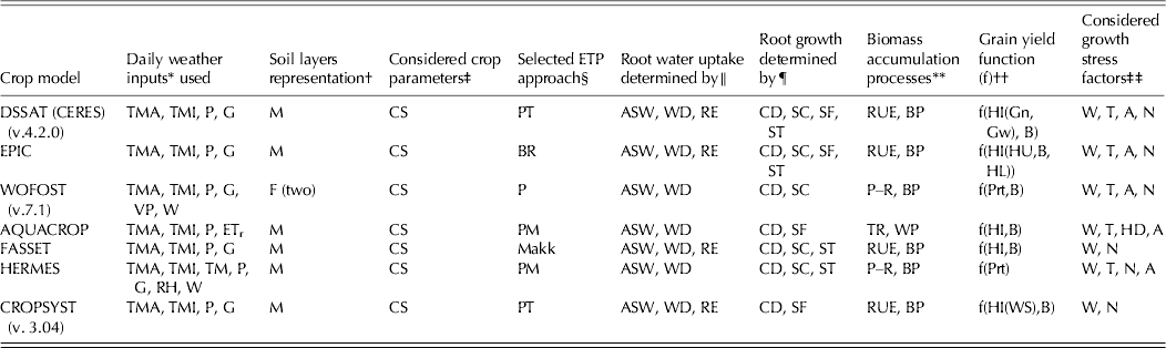
The crop simulation models considered in the present study are DSSAT (CERES-Wheat and CERES-Maize), (Jones et al. Reference Jones, Hoogenboom, Porter, Boote, Batchelor, Hunt, Wilkens, Singh, Gijsman and Ritchie2003; Porter et al. Reference Porter, Hoogenboom, Batchelor, Jones and Gijsman2003; Hoogenboom et al. Reference Hoogenboom, Jones, Porter, Wilkens, Boote, Batchelor, Hunt and Tsuji2004; Timsina & Humphreys Reference Timsina and Humphreys2006; Vučetić Reference Vučetić2011), EPIC (Williams et al. Reference Williams, Jones and Dyke1984; Williams Reference Williams and Singh1995; Izaurralde et al. Reference Izaurralde, Williams, Mcgill, Rosenberg and Quiroga Jakas2006), WOFOST (Boogaard et al. Reference Boogaard, Van Diepen, Rötter, Cabrera and Van Laar1998; van Ittersum et al. Reference Van Ittersum, Leffelaar, Van Keulen, Kropff, Bastiaans and Goudriaan2003), AQUACROP (Hsiao et al. Reference Hsiao, Heng, Steduto, Rojas-Lara, Raes and Fereres2009; Raes et al. Reference Raes, Steduto, Hsiao and Fereres2009; Steduto et al. Reference Steduto, Hsiao, Raes and Fereres2009), FASSET (Jacobsen et al. Reference Jacobsen, Petersen, Berntsen, Boye, Sørensen, Søgaard and Hansen1998; Olesen et al. Reference Olesen, Jørgensen and Mortensen2000, Reference Olesen, Berntsen, Hansen, Petersen and Petersen2002a, Reference Olesen, Petersen, Berntsen, Hansen, Jamieson and Thomsenb), HERMES (Kersebaum & Beblik Reference Kersebaum, Beblik, Shaffer, Ma and Hansen2001; Kersebaum Reference Kersebaum2007) and CROPSYST (Stockle et al. Reference Stockle, Donatelli and Nelson2003). All of these models have been already implemented in model inter-comparison studies, where further details can be found (Eitzinger et al. Reference Eitzinger, Trnka, Hösch, Žalud and Dubrovský2004; Todorovic et al. Reference Todorovic, Albrizio, Zivotic, Abi Saab, Stockle and Steduto2009; Palosuo et al. Reference Palosuo, Kersebaum, Angulo, Hlavinka, Moriondo, Olesen, Patil, Ruget, Rumbaur, Takác, Trnka, Bindi, Çaldag, Ewert, Ferrise, Mirschel, Saylan, Siska and Rötter2011). All models have in common daily time-step simulation with daily weather as input. They differ mainly in the details given in the soil and crop parameter inputs and the related representation of the various simulated processes. Table 1 provides an overview of the various crop models applied in the present study, indicating basic modelling concepts.
Crop models applied for winter wheat and maize and the key model characteristics which are most relevant for the results in the present study (modified, after Palosuo et al. Reference Palosuo, Kersebaum, Angulo, Hlavinka, Moriondo, Olesen, Patil, Ruget, Rumbaur, Takác, Trnka, Bindi, Çaldag, Ewert, Ferrise, Mirschel, Saylan, Siska and Rötter2011)

* TMA, maximum air temperature; TMI, minimum air temperature; TM, mean air temperature; P, precipitation; G, global radiation; RH, mean relative air humidity; VP, early morning vapour pressure; W, wind speed; ETr, reference evapotranspiration (grass as reference crop, as a function of temperature, relative humidity, global radiation and wind speed).
† Soil inputs consider variable, multiple soil layers (M) or only fixed, few soil layers (F).
‡ Cultivar-specific genetic coefficients (CS).
§ Selected evapotranspiration (ETP) approach: BR, Baier–Robertson; Makk, Makkink; P, Penman; PM, Penman–Monteith; PT, Priestley–Taylor.
∥ ASW, available water in the root zone; WD, actual crop water demand; RE, soil and root water uptake resistances.
¶ CD, crop development; SC, physical soil conditions; ST, soil temperature; SF, stress factor (water).
** RUE, radiation use efficiency approach; BP, biomass partitioning; P–R, Explanatory approach (Gross photosynthesis–respiration); TR, transpiration; WP, normalized water productivity.
†† HI, harvest index; B, above ground biomass; Prt, partitioning during reproductive stage; HU, heat unit; HL, harvest losses; Gn, genetical fixed grain number; Gw, genetical fixed potential kernel weight; WS, water stress factor (actual/potential evapotranspiration).
‡‡ W, water; T, limiting extreme temperatures; N, nutrients; A, soil aeration; HD, direct heat effects (e.g. pollination).
As the present study mainly addresses the effects of simulated drought and heat stress on crop yield, the deviation in model results might be explained by differences in the way that related processes are represented in the models (Table 1). In the case of soil and crop water balance, processes such as the type of soil-water balance simulation, the root growth and crop water uptake process are crucial. Although all models use the capacitive approach for soil water simulation, differences occur in the selected evapotranspiration equations, representation of soil layers (WOFOST allows only two soil layers) and in the critical thresholds when water uptake will be reduced, as well as how this process is described. The root growth processes are also simulated differently, which can lead to significant accumulating differences in the available soil water over the growing period (Eitzinger et al. Reference Eitzinger, Trnka, Hösch, Žalud and Dubrovský2004).
All models included in the present study consider the effect of high temperatures on yield formation process to some extent, but there are also different thresholds described and applied partly on different growth processes (e.g. on partitioning if this process was simulated). Also, only some of the models have the capability to re-allocate assimilates from stem to grains during grain-filling, which can be one reason for large yield reductions under drought conditions. Only AQUACROP considers the direct effect of heat stress (on pollination) which can be an important yield-reducing factor under extreme weather conditions (heat and drought).
Study sites and selected years
Two sites in different climatic regions in Austria were selected for the crop model inter-comparison and sensitivity analysis.
The first site (site A) in Raasdorf (48°14′N, 16°34′E, 152 m a.s.l.) is located in the Marchfeld region of north-eastern Austria, which is not only one of the major field crop production areas, but also one of the driest regions in the country. Marchfeld is a plain of c. 1000 km2 with minor variations in elevation, ranging from 143 to 178 m. The region is influenced by a semi-arid, continental climate. The annual mean temperature, averaged over 1971–2000, was 9·8°C with a mean annual precipitation of 520 mm (representative weather station Gross-Enzersdorf, 48°12′N, 16°33′E, 157 m a.s.l.). The dominating soil type in this area is classified as calcic chernozem (FAO-UNESCO 1988), explicitly as chernozem on fine calcareous sediments over gravel and sand.
The second site (site B) in Paurach (46°57′N, 15°49′E, 290 m a.s.l.) is located in another intensively used agricultural region dominated by arable cropping in the south-eastern part of Austria and south of the Alps. The topography is characterized by flat valleys broken by gently rolling terrain and hills. The climate in this region (Prettenthaler et al. Reference Prettenthaler, Podesser and Pilger2010) is influenced by both Mediterranean and continental climates with warm summers and mild winters, and is in general more humid and less windy than the Marchfeld region. The mean annual temperature, averaged over 1971–2000, was 8·4°C with a mean annual precipitation of 817 mm (representative weather station Gleisdorf, 47°6′N, 15°42′E, 365 m a.s.l.). The dominating soil type in this study area is classified as a gleyic cambisol (FAO-UNESCO 1988).
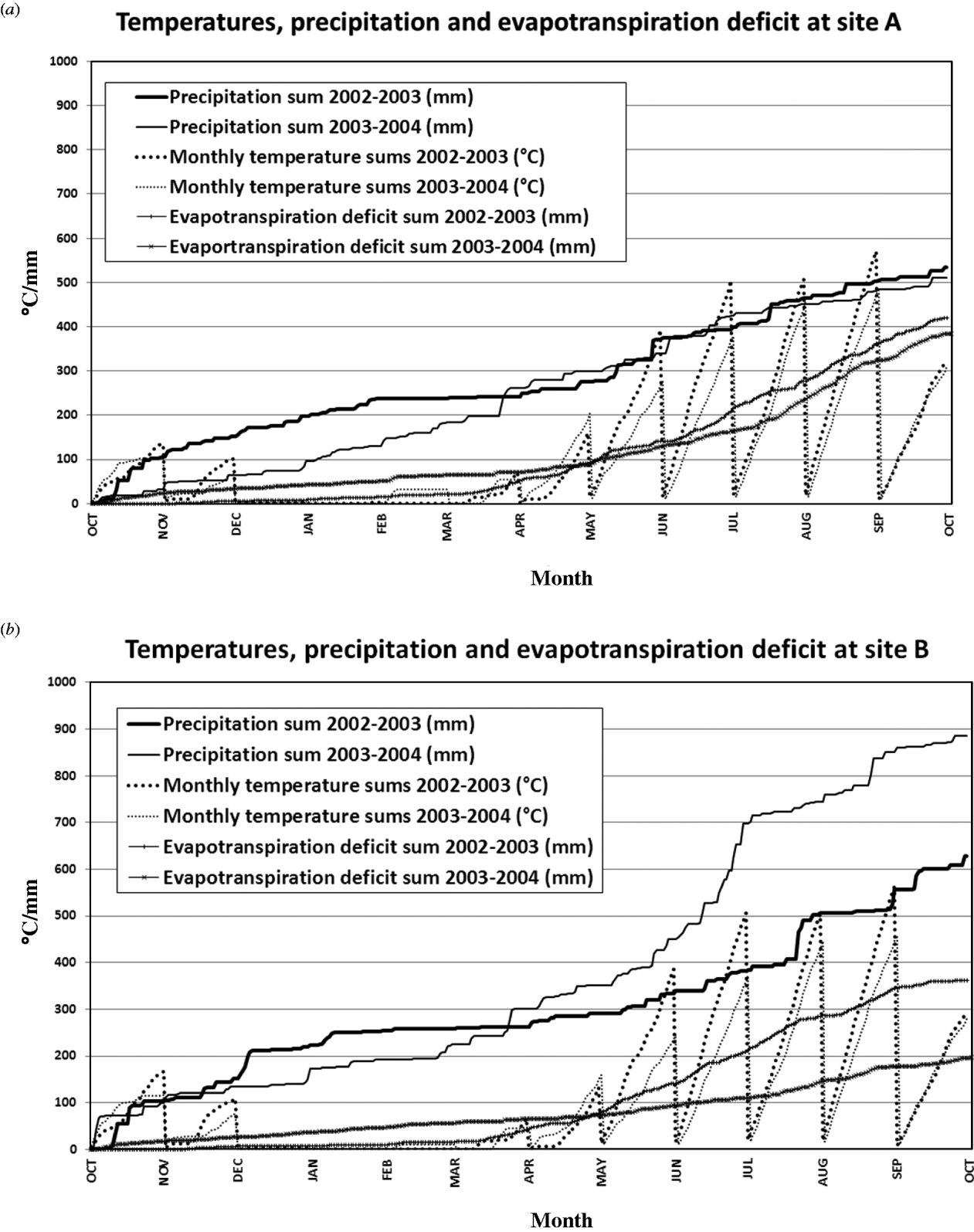
Two years with contrasting weather conditions (2003 and 2004) were considered for the sensitivity analysis for both the winter wheat and maize growing periods (Fig. 1). The weather during summer 2003 was exceptional in central Europe and very different from 2004. In general, summer 2003 at both sites was characterized as warm with some hot spells and dry periods, and 2004 as very humid and cooler than 2003 without any drought or heat stress periods for crops. In 2004, lower temperature sums were reached at both locations during growing periods for both winter wheat and maize. For most months, lower temperature sums were achieved at site B than at site A, reflecting the overall climatic differences between the sites. In 2003 especially, precipitation from February to June was below normal at both sites. The precipitation during the growing season (April–September) was similar between 2003 (294 mm) and 2004 (255 mm) at site A, except for June (21 mm) which was very dry and hot in 2003. At site B, the precipitation during the growing season (April–September) differed considerably between the years, with only 365 mm in 2003 compared with 587 mm in 2004. Global radiation sums during the growing periods (Figs 1(a) and (b)) differed less than 3% between the two sites in both years; however, in 2004, it was lower by c. 4% at site A and by c. 8% at site B compared with that of their respective sites in 2003.
Monthly temperature sums (accumulated mean daily temperatures >5°C), precipitation sums and accumulated evapotranspiration deficit for (a) site A and (b) site B, over the growing periods of winter wheat and maize 2002/03 and 2003/04. Evapotranspiration deficit is calculated as grass reference evapotranspiration minus actual evapotranspiration for grass according to the approach of Allen et al. (Reference Allen, Pereira, Raes and Smith1998).
Design of the weather and soil scenarios
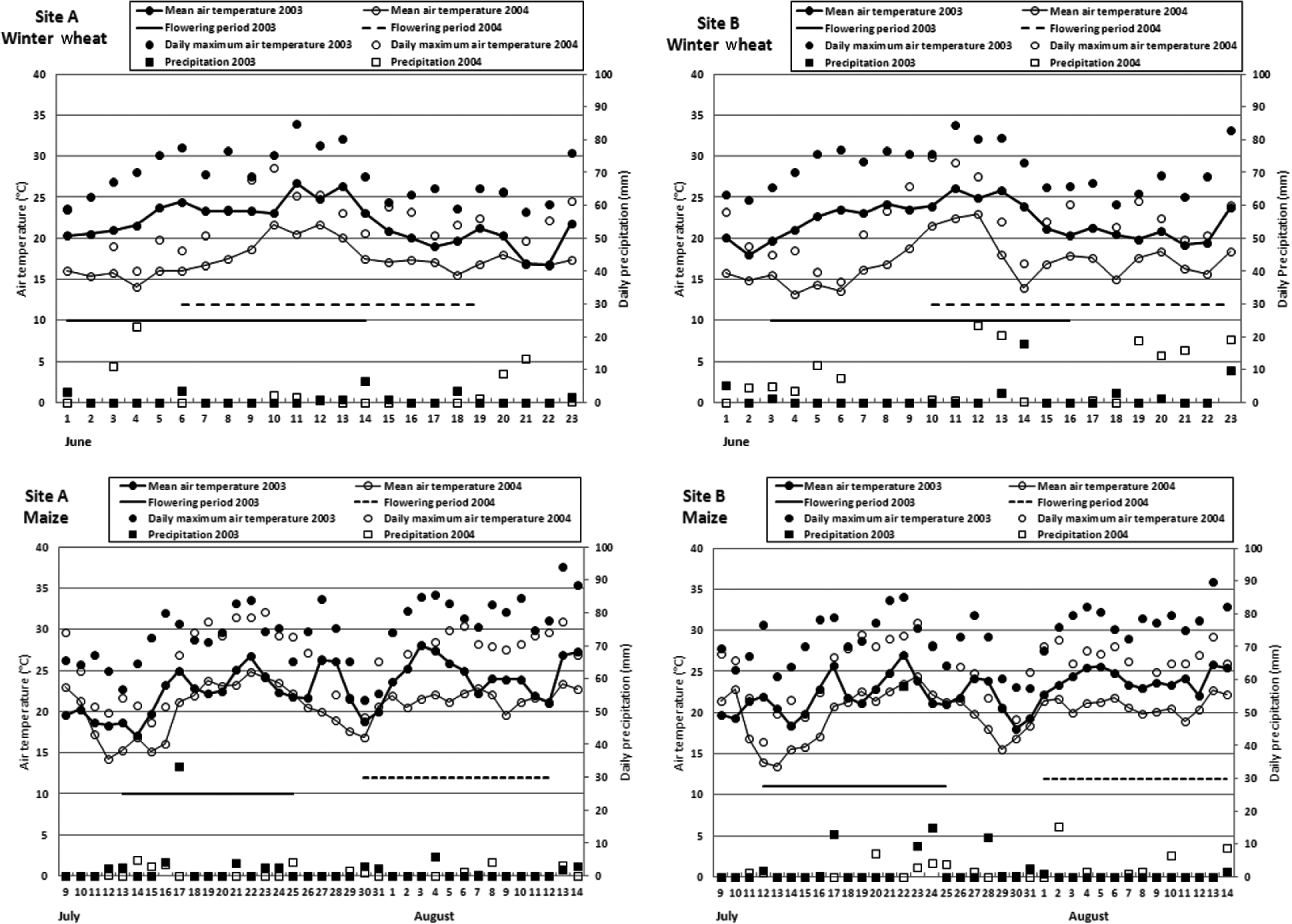
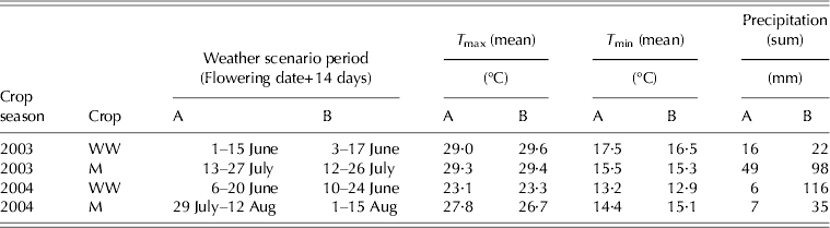
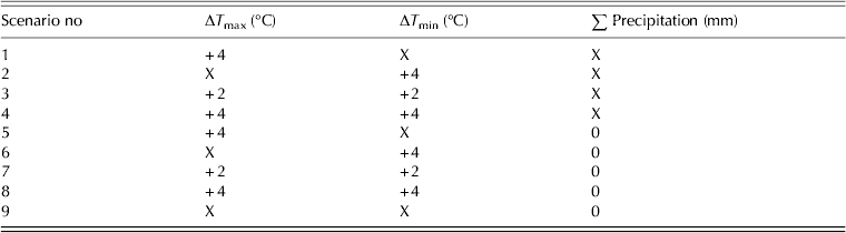
Weather scenarios for the two locations and years were developed by modifying daily temperature and precipitation during the observed very sensitive flowering period (defined as start of flowering+14 days), critical for yield formation in maize and winter wheat (Fig. 2, Table 2(a). Daily maximum and/or minimum temperatures were increased by 2 or 4°C in combination with the observed precipitation or the precipitation set to zero (resulting in nine different combinations; Table 2(b)). The selected temperature increments reflect a probable range of increase in mean temperatures projected to 2100 and decreasing summer precipitation/increasing drought frequencies were based on regional climate scenarios projected for Central Europe (Trnka et al. Reference Trnka, Eitzinger, Dubrovsky, Semeradova, Stepanek, Hlavinka, Balek, Skalak, Farda, Formayer and Zalud2010).
Course of the daily temperatures and precipitation for the 14-day periods of the sensitivity analysis of maize and winter wheat (flowering periods) in 2003 and 2004 at the two Austrian sites (in the 14-day flowering period, the weather scenarios shown in Table 2(b)) are applied).
Weather conditions during the scenario period (flowering date +14 days) of maize and winter wheat at the two sites and 2 years (baseline, representing the measured conditions)
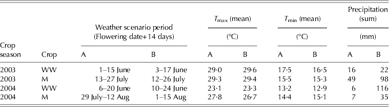
T max, maximum air temperature; T min, minimum air temperature.
M, maize; WW, winter wheat.
A, location Raasdorf (Lower Austria); B, location Paurach (Styria).
Weather changes during the scenario periods (flowering date +14 days, Fig. 1) applied on daily basis for the crop model sensitivity analysis during the flowering period of maize and winter wheat v. the baseline (observed weather, see Table 2(a))
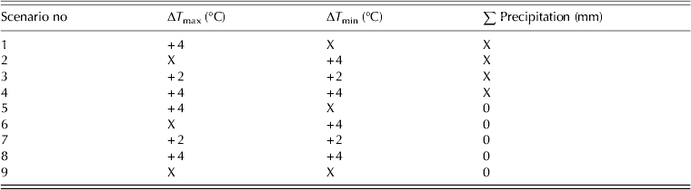
X, unchanged observed weather (Table 2(a)).
By applying the weather scenarios with an increase in daily temperatures, temperature sums were consequently increased during the flowering period (2 weeks). For the baseline (measured) conditions during winter wheat flowering at both sites, maximum daily temperatures reached 35°C in 2003 and 30°C in 2004 (Fig. 2). For maize during flowering at both sites, maximum daily temperatures also reached 35°C in 2003 and 33°C in 2004. Mean maximum daily temperatures of c. 29–30 and 31–32°C, respectively, were reached during the 2-week flowering period of winter wheat and maize in both years, in the case of +4°C increase in daily maximum temperatures (scenario 1; Table 2(b)).
In 2003, precipitation during the flowering period was 16 mm at site A and 22 mm at site B for winter wheat and 49 mm at site A and 98 mm at site B for maize. In 2004, the precipitation at site A was only 6 mm and at site B it was 116 mm for winter wheat, and 7 mm at site A and 35 mm at site B for maize (Fig. 2). In the weather scenarios 5–9, the precipitation during the flowering period for 2 weeks was set to zero.
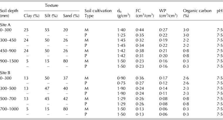
In addition, physical soil properties across soil layers at each site were set for two different types of tillage options: conventional tillage (mouldboard plough; cultivation depth 250 mm) and minimum tillage (disc harrow; cultivation depth 50–100 mm). In particular, the physical soil properties for each tillage practice were estimated from field experiments (Rischbeck Reference Rischbeck2007; Hlavinka et al. Reference Hlavinka, Eitzinger, Smutny, Thaler, Zalud, Rischbeck and Kren2010; Thaler et al. Reference Thaler, Eitzinger, Trnka and Dubrovsky2012) and applied to three parameters only: bulk density, field capacity and wilting point (Table 3). In general, significantly higher available soil water contents in the top soil layer (0–900 mm) are given for minimum tillage than for ploughing. The physical soil parameters used as input for crop models of both study sites (and for two types of tillage practices) are shown in Table 3. In the simulations no capillary rise from a groundwater table have been considered, which reflects the real conditions at both selected sites. Further, all crop models were set to the current ambient CO2 level of 380 ppm for the simulations.
Basic soil properties at the two Austrian sites including the modifications for type of tillage practice (Rischbeck Reference Rischbeck2007) representing the crop model inputs
db, bulk density (g/cm3); M, mulchboard drilling; P, plough; FC, field capacity; WP, wilting point.
Model inter-comparison
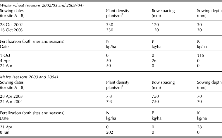
The model comparisons in the present study were made with limited model calibration by using fixed sowing dates and crop management practices (Table 4) and fitting model simulated phenology to observed main phenological events, such as flowering date (Table 2(a)) and physiological maturity for both winter wheat and maize. For these phenological stages, a deviation of maximum 3 days to the reported date was a precondition (except EPIC for flowering, because it does not simulate timing of flowering explicitly), which is normally accepted for successful model calibration or validation. In this way it was ensured that the simulated flowering period was well within the 2 weeks weather scenario period after flowering date. No model validation on absolute experimental yields or cultivar-specific characteristics was carried out, thus the study results should not be justified on absolute simulated grain yields. The main aim of the present study, however, was to compare the simulated yield deviations and the models sensitivities with increased temperatures and reduced precipitation (weather scenarios) during the sensitive flowering period and under different weather and soil conditions (two different soils and two tillage options).
Key management settings for winter wheat and maize simulations for both sites and years applied for all scenarios
RESULTS
Crop model responses under baseline conditions
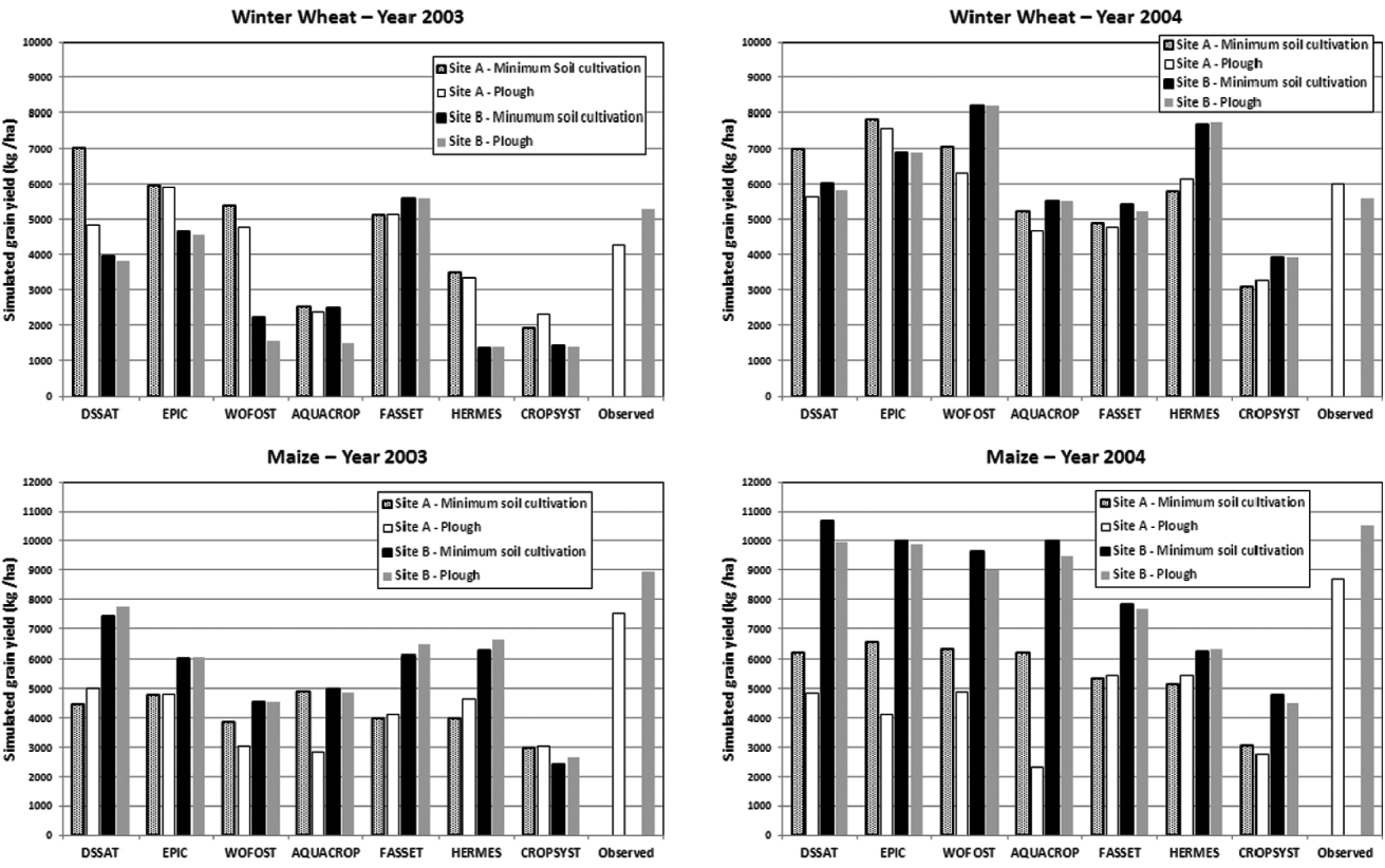
The observed mean regional yields (mean yields of the federal districts of Lower Austria and Styria as reported by Statistics Austria (2004, 2005)) and their differences between sites and years are shown in Fig. 3. The observed regional yields are not related to tillage practices, where tillage after ploughing in autumn is dominant in both regions. They represent the influence of the mean weather differences between the 2 years in these two climatic regions, whereas the simulations are based on the data of only one weather station at each site. Therefore, and due to other potential deviations from the simulation settings, some bias in the yield level can be expected. In the case of site A, which is located in the driest area of the whole region of Lower Austria, maize is mostly irrigated during dry periods, which leads to significantly lower simulated rainfed maize yields. For this reason, the observed regional yields should not be used for a direct evaluation on the absolute simulated yields. In 2003, both crops showed higher observed yields of c. 1000 kg/ha within the more humid region of site B. This finding is also supported by the differences in accumulated precipitation and the evapotranspiration deficit between measurement sites (Figs 1(a) and (b)). In the wetter and cooler 2004 (Figs 1(a) and (b)), only maize showed higher observed yields (1810 kg/ha) within the region of site B (Styria), but winter wheat had lower yields (420 kg/ha) compared with the region of site A (Lower Austria). Figure 3 further shows that the crop models considered in the present study vary widely (more than 100%) in simulating the absolute yield levels, which is not surprising since no model calibration and validation on crop grain yields have been carried out.
Simulated winter wheat and maize yields of the crop models for the baseline (unchanged weather conditions of 2003 and 2004) at the two sites in Austria including two types of tillage practice. Observed yields represent regional yield statistics of federal districts ‘Lower Austria’ and ‘Styria’ (Statistics Austria 2004, 2005), where tillage after ploughing in the autumn dominates.
The models, however, agree with some exceptions in the simulated yield trends for both maize and winter wheat among sites, years and soil tillage practices. In the drier and hotter year of 2003, for example, most models simulate considerably lower yields at both sites for winter wheat than in 2004 (except by FASSET and DSSAT for site A). This overall trend is confirmed by the observed yield statistics for both years (Fig. 3). The models simulate distinctly higher yields for maize only at site B in 2004, except for HERMES. The simulated maize yields at site A are more similar between 2003 and 2004, especially for the ploughed treatment. Also, in this case the overall trend of the yield difference between the 2 years is confirmed by the observed data.
A clear common trend can be seen for the site effect between the crop models for maize during both years (though less pronounced in 2003), where significantly higher yields are simulated for site B (except by CROPSYST in 2003). This overall trend is confirmed by the observed regional yields. For winter wheat in 2003 higher yields are simulated at site A (except by AQUACROP and FASSET), whereas in 2004 most models simulate higher yields at site B than at site A (mixed responses). In this case, the overall trend is different than in the observed regional yields.
Furthermore, the models show sensitivity to the tillage practice (or the soil physical properties driven by the tillage operations), but the model responses (increase or decrease in yield) are more mixed. For example, most models (except CROPSYST at site A) simulate higher yields for winter wheat in 2003 for minimum tillage, but with large variation in the yield differences between models and sites. For maize in 2003, however, the response to the tillage practice between models and sites is mixed. For site A the simulated maize yield differences between plough and minimum tillage are higher in 2004 than in 2003. At both sites and in most cases higher yields are simulated under minimum tillage for both maize and winter wheat in 2004 (with a total range of −350 to +3837 kg/ha).
The agreement of the model response to the effect of tillage practice is better in 2004 for both crops, whereas in most cases moderately higher yields (100–1000 kg/ha) are simulated for minimum tillage. At site A, slightly more water stress occurred in 2003 than in 2004 for maize (Fig. 1(a)), but this leads to more mixed model responses in 2003 than in 2004. This behaviour at both sites contradicts the general assumption that minimum tillage may increase yields under drier conditions by increasing soil-water storage capacity (Table 3).
Model behaviour under different stress scenarios
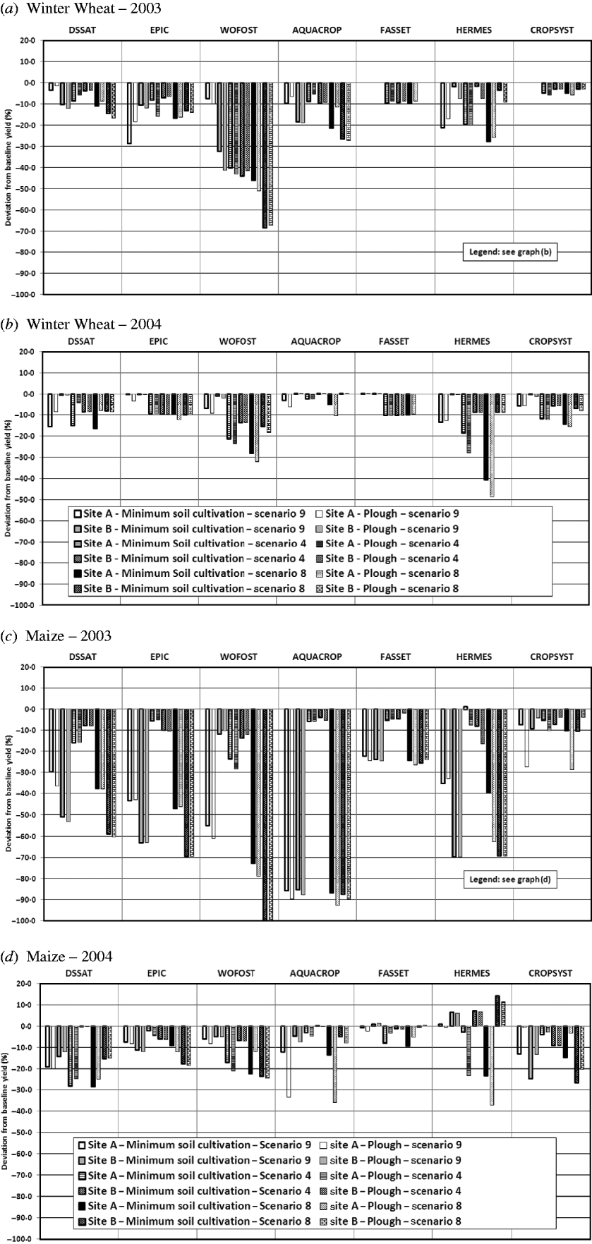
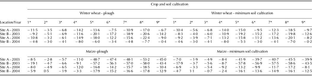
The ensemble means of the simulated crop yield deviations from the baseline yield are shown in Table 5 for each weather scenario. In general, nearly all models predict a reduction in crop yields for these scenarios (Table 2(b))), except in a few cases where yields increased marginally compared with the baseline yields (Fig. 4). In the ensemble mean, scenario 8 mostly shows the highest reduction in simulated yields and scenario 2 the lowest. The scenarios of each parameter combination (change in temperatures only, change in temperature and precipitation, change in precipitation only) with the most significant model responses (scenarios 4, 8 and 9 as shown in Table 5) are shown in Figs 4(a–d) for each model and are discussed further below. Scenario 4 represents an increase in both minimum and maximum temperatures by 4°C, scenario 8 represents scenario 4 but with no precipitation and scenario 9 represents no changes to temperatures but with no precipitation during the 2-week period after the start of flowering for both crops.
(a) Relative deviations of simulated winter wheat grain yields of selected weather scenarios 4, 8 and 9 (Table 2(b)) from the baseline in 2003. (b) Relative deviations of simulated winter wheat grain yields of selected weather scenarios 4, 8 and 9 (Table 2(b)) from the baseline in 2004. (c) Relative deviations of simulated maize grain yields of selected weather scenarios 4, 8 and 9 (Table 2(b)) from the baseline in 2003. (d) Relative deviations of simulated maize grain yields of selected weather scenarios 4, 8 and 9 (Table 2(b)) from the baseline in 2004.
Ensemble means of all seven crop models’ simulated yield deviations (in percentage) from the simulated baseline yields (Fig. 2) for each scenario
* Scenario number according to Table 2(b)) (no. 1–4 represent an increase in temperatures only; No. 5–8 represent a combination of 1–4 and no precipitation; no. 9 represent no precipitation – all changes during the 2 weeks flowering period).
Simulated winter wheat yields for selected weather scenarios at both sites for ploughing
In 2003 at site A, EPIC, WOFOST and HERMES simulated decreases in yield exceeding 10% in scenario 4 (caused by increased temperatures of 4°C only), with WOFOST simulating the largest decrease in yield (43%). At site B, only WOFOST showed yield decrease exceeding 10%, showing a similar response as for site A. In 2004 at site A, WOFOST, HERMES and CROPSYST simulated yield decreases larger than 10%, with HERMES showing the maximum (28%). At site B, only WOFOST simulated yield reductions slightly exceeding 10% in 2004. Between 2003 and 2004, all the models except WOFOST showed differences in the relative response of less than 10% for both sites.
For scenario 9 (omitted precipitation only), yield decreases of more than 10% at site A in 2003 were seen only for EPIC and HERMES, in general reflecting the relatively small amount of baseline precipitation recorded during this period. At site B, however, all the models except FASSET, HERMES and CROPSYST simulated decreases in yield exceeding 10%, with WOFOST showing the maximum of 41%. For 2004, only HERMES showed yield reduction exceeding 10% at site A. At site B in 2004, all the models agreed very well with almost no change in simulated yields which can be explained by the very wet soil conditions before the flowering period at this site. Between 2003 and 2004, FASSET, HERMES and CROPSYST showed simulated relative yield differences of less than 10% for both sites.
Scenario 8 (combined effect of increased temperatures and omitted precipitation) caused the highest decrease in simulated yields in the ensemble mean. For 2003 at site A, EPIC, WOFOST, AQUACROP and HERMES showed yield reductions exceeding 10% with WOFOST simulating the maximum decrease (51%), which reflects well the temperature responses of scenario 4. At site B in 2003, only FASSET, HERMES and CROPSYST simulated yield decreases lower than 10%, whereas WOFOST showed the maximum of 67% reduction in yield. In 2004 at site A, DSSAT and FASSET only had yield reductions of less than 10%, with the highest shown by HERMES (49%). At site B in 2004, WOFOST showed only 18% reduction in yield. Between 2003 and 2004, DSSAT, EPIC, FASSET and CROPSYST showed simulated relative yield differences of less than 10% for both sites.
Effect of tillage practice on simulated winter wheat yields at sites A and B
In general, the deviations in simulated yields between ploughing and minimum tillage range between 0 and 10% for all models and in both years. However, the direction of these deviations depends on the weather scenario and on the year for each model, and is different between the models as well.
At site A in 2003, DSSAT, AQUACROP and HERMES showed higher reductions in simulated yields for minimum tillage for all three scenarios (4, 8 and 9), but in general the opposite response was seen for site B. EPIC shows the same behaviour, except for scenario 4. FASSET and CROPSYST show only marginal differences between tillage practices, combined with the generally low yield response to the scenarios. WOFOST showed higher yield losses for the ploughed variant, except at site B for two of the scenarios. In 2004, only DSSAT at site A showed significantly higher yield losses in all scenarios for minimum tillage (at site B the differences are marginal). All other models showed higher or very similar yields for ploughing, whereas for EPIC, AQUACROP, FASSET and CROPSYST the differences were less pronounced.
Simulated maize yields for selected weather scenarios at both sites for ploughing
In 2003 at site A, WOFOST and DSSAT simulated more than 10% reduction in yield for scenario 4 (caused by increased temperatures only), where WOFOST showed the strongest response with 28% reduction in yield. At site B the model responses were more uniform where EPIC, HERMES and WOFOST showed decreases in yield slightly exceeding 10%.
In 2004 at site A, DSSAT, WOFOST and HERMES showed yield reductions greater than 10% (20–25%). At site B in 2004, with very wet and cooler conditions during the growing season than in 2003 (Fig. 1), all the models showed yield decreases in the range of 0–10%, except HERMES which simulated yield increase of 7%. Between 2003 and 2004, all models except DSSAT and HERMES showed simulated relative yield differences of less than 10% for both sites.
Looking at scenario 9, showing the effect of omitted precipitation only, all the models simulated a significant yield reduction well above 10% for 2003 at site A, ranging widely from 24 (FASSET) to 90% (AQUACROP). At site B in 2003, only CROPSYST showed less than 10% yield reduction, while all other models responded with a wide range of yield reduction, from 10 (WOFOST) to 79% (AQUACROP). For 2004, only DSSAT and AQUACROP showed yield reductions exceeding 10% at site A. At site B in 2004, the modelled yield changes ranged from +6 (HERMES) to −13% (CROPSYST). Between 2003 and 2004, only WOFOST and CROPSYST showed simulated yield differences of less than 10% and only for site B.
Scenario 8 (combined effect of increased temperatures and skipped precipitation) caused, as in the case of winter wheat, the highest simulated yield decreases in the ensemble mean. For 2003 at site A, all the models simulated significant reductions in yield exceeding 10% and ranging from 26 (FASSET) to 93% (AQUACROP). At site B in 2003, the ensemble mean yield decreases were even higher and ranged more widely, from −4% for CROPSYST and −100 for WOFOST. The other models were in the range of −24 to −80%. The same response was seen for WOFOST in this scenario in the case of winter wheat. In 2004 at site A, only FASSET and CROPSYST showed yield reductions below 10% while the highest reduction of 37% was simulated by HERMES (similarly to winter wheat). At site B in 2004, all models exceeded 10% yield reduction except for AQUACROP, FASSET (+1%) and HERMES (+12%). Between 2003 and 2004, all models showed simulated relative yield differences above 10% for both sites.
Effect of tillage practices on simulated maize yields at sites A and B
The deviations in simulated yields between ploughing and minimum tillage for most cases ranged from 0 to 10%. There were some significant exceptions in comparison with winter wheat, however, as some models for some scenarios showed deviations in simulated yield responses of up to 20%, especially in 2004. As for winter wheat, the direction of these deviations depended on both the scenario and the year for each model, and it also varied between models.
At site A in 2003, the models in most cases showed either a decrease or no change in simulated yields for ploughing compared with minimum tillage for all three scenarios (4, 8 and 9) and both sites. At site B only CROPSYST, FASSET and HERMES showed different responses with lower yields for minimum tillage in some of the three scenarios. The EPIC model showed slightly lower yields for minimum tillage at both sites and for all three scenarios. In general EPIC, DSSAT and FASSET showed the lowest responses to tillage practices, and WOFOST, HERMES and CROPSYST showed more pronounced differences in 2003.
In 2004, the model responses were more inconsistent. In most cases DSSAT showed slightly lower yields for minimum tillage, and EPIC for ploughing (in contrast to 2003 in both cases). WOFOST, compared with 2003, changed its behaviour only for site A and scenario 8 with a significantly lower yield for minimum tillage. AQUACROP did not change its behaviour (lower yield for ploughing) but simulated much higher yield differences especially for scenarios 9 and 8. FASSET also responded in a similar way in 2003 with one exception (similar to WOFOST). HERMES in most cases showed similar responses in 2004 to 2003, i.e. lower yields for the plough variant, whereas CROPSYST behaved differently compared with 2003. In general EPIC, DSSAT and FASSET showed the lowest responses to the two tillage practices, whereas AQUACROP, HERMES and CROPSYST showed more pronounced differences in 2004.
Model response to simulated available soil water
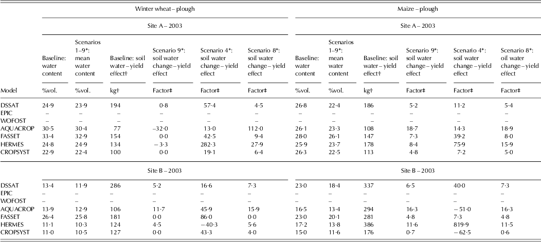
Table 6 shows some indicators for the models, providing detailed outputs in terms of soil water content in 2003. These indicators reflect the simulated soil water content–yield relationships of the baseline and the effect of soil water change on differences in simulated yield.
Simulated soil water contents (%vol.; 0–300 mm) of the crop models (where available) for the baseline and the scenarios during the flowering periods in 2003 and the relation to simulated absolute yields in the baseline scenario and to scenario yield changes for maize and winter wheat
* Scenarios (Table 2): Scenario 9, skipped precipitation; scenario 4, increase of T max and T min by 4°C; Scenario 8, combination of scenarios 9 and 4.
† Simulated grain yield (kg/ha) per %vol. soil water content.
‡ Factor, relative yield change (%)/change in soil water content (%vol.); high factor values show low-yield change response to change in soil water content and vice versa; positive values show that yield and water content change have the same trend (positive or negative) and vice versa.
The simulated mean soil water content of the top soil layer (0–300 mm) during the flowering period of both crops for the baseline and the mean of the weather scenarios differed considerably between the crop models, although they agreed in general trends considering different sites and crops as well as wetter or drier conditions. In most cases, CROPSYST showed the lowest simulated soil water contents, whereas AQUACROP generally showed the highest values. Regarding the relationship of simulated available soil water content and yield, DSSAT showed the highest value and AQUACROP the lowest (with one exception for maize at site B) in most cases.
For scenarios 4, 8 and 9 (Table 2(b)), the effect on simulated yield change due to soil water change during the flowering period was assessed. Homogeneous model responses were found for maize at site A and in some models for winter wheat at site B. The general trend and degree of responses varied most for maize at site B and for winter wheat at site A. Site A in 2003 showed higher soil water contents for maize, which were also more uniform between the models. Thus, it was concluded that the models agreed better under unstressed growing conditions in the case of maize. The biggest variations among the models for both crops and sites were obviously in scenario 4 (temperature changes only), whereas the best agreements were seen for scenario 9 (skipped precipitation only). This indicates that the models responded differently to changing temperature, adding even more uncertainty to simulated crop yield (which can be seen by comparing scenarios 8 and 9 in Table 6).
DISCUSSION
Understanding modelled sensitivities of crop growth and yield prediction related to changes in environmental parameters such as weather conditions is essential for their judicious use in both large area applications and in predicting the effects of future environmental changes (Nonhebel Reference Nonhebel1993; Semenov & Porter Reference Semenov and Porter1995; Trnka et al. Reference Trnka, Žalud, Eitzinger and Dubrovský2005; Rötter et al. Reference Rötter, Carter, Olesen and Porter2011). Inter-comparison of different modelling approaches and models can reveal the strengths and weaknesses of models and display uncertainties related to their application. Variation of model results in model inter-comparisons also comprises the uncertainty resulting from the way processes are simulated, which is most difficult to quantify (Chatfield Reference Chatfield1995).
In the present study, the model responses to nine weather scenarios of increased temperatures (and heat stress) and reduced precipitation (and drought stress) for a period of 2 weeks during flowering for winter wheat and maize were determined and compared. The soil and weather data of the baseline included real conditions of two contrasting sites and years in Austria. The results of the study showed that the model responses in general agreed on the direction of yield change (positive or negative) between the baseline and the scenarios.
The sensitivity of the models to increased temperature and decreased precipitation varied, although they followed similar trends in simulated crop yields (except HERMES and FASSET for maize in 2004). The lowest sensitivities to the weather scenarios in general were obtained for FASSET and CROPSYST.
The lower sensitivity of maize in FASSET may be due partly to crop transpiration and the effects of drought not being correctly simulated for this crop. The response of the maize model in FASSET has not previously been calibrated for sites outside of Denmark.
The lower sensitivity of CROPSYST to manipulated weather parameters, for example, may be ascribed to the limited calibration of the crops under the climatic and soil conditions of sites in Austria, which left out important parameters (e.g. radiation and water use efficiency) and greatly affected crop growth and yield. The lower yields simulated with the baseline are the consequence of lower above ground biomass produced during the growing cycle revealing sub-optimal environmental conditions, so that more stressful conditions cannot produce more deviations in response.
WOFOST, and to a certain extent AQUACROP and HERMES, were the most sensitive to differences among the defined weather scenarios, and also to differences between sites. It has already been shown that WOFOST is quite sensitive to soil differences (sites) as it relies on just two layers and very few soil parameters. Furthermore, the model is also quite sensitive to soil water deficits, whereas so far, it is not known to be particularly sensitive to ‘heat stress’ (Rötter et al. Reference Rötter, Palosuo, Kersebaum, Angulo, Bindi, Ewert, Ferrise, Hlavinka, Moriondo, Nendel, Olesen, Patil, Ruget, Tacak and Trnka2012).
Effects of temperatures
The response to increased temperatures in the applied scenarios (Fig. 2) varied greatly among the models and these differences changed with the respective crop. For example, WOFOST showed large reduction in yield under increased temperatures for winter wheat (especially in 2003, Fig. 4(a)), while for maize DSSAT and WOFOST showed the highest, but compared with winter wheat more moderate reductions (Figs 4(c–d)). These differences can be attributed to the different cultivar-specific calibrations but also to different temperature response algorithms in the models (Porter & Semenov Reference Porter and Semenov2005; Asseng et al. Reference Asseng, Foster and Turner2011; Nendel et al. Reference Nendel, Berg, Kersebaum, Mirschel, Specka, Wegehenkel, Wenkel and Wieland2011; Palosuo et al. Reference Palosuo, Kersebaum, Angulo, Hlavinka, Moriondo, Olesen, Patil, Ruget, Rumbaur, Takác, Trnka, Bindi, Çaldag, Ewert, Ferrise, Mirschel, Saylan, Siska and Rötter2011; Rötter et al. Reference Rötter, Carter, Olesen and Porter2011, Reference Rötter, Palosuo, Kersebaum, Angulo, Bindi, Ewert, Ferrise, Hlavinka, Moriondo, Nendel, Olesen, Patil, Ruget, Tacak and Trnka2012; White et al. Reference White, Hoogenboom, Kimball and Wall2011), including physiological response functions and probably also evapotranspiration, depending on the method used. For example, in the case of DSSAT based CERES-Wheat, the growing temperature thresholds are 0 and 26°C and in CERES-Maize 8 and 34°C.
In spite of large differences in the temperature response observed in the present results, the direct effect of heat stress impact in the short time period around flowering is in most cases (except AQUACROP) not considered by the models included in the present study. In AQUACROP, heat stress during pollination of maize and wheat is considered using a critical limit of 40–45 and 35–40°C, respectively, where the critical limit is reached in the weather scenarios 4 and 8 for winter wheat in 2003 (exceeding maximum temperatures of 35°C during flowering). The fact that direct heat effects are often not considered in models has the potential to cause even higher deviations between simulated and observed yields in many studies (Asseng et al. Reference Asseng, Foster and Turner2011; Moriondo et al. Reference Moriondo, Giannakopoulos and Bindi2011; Rötter et al. Reference Rötter, Carter, Olesen and Porter2011).
Another problem related to the heat effect on crops is that in extreme temperatures the crop models normally consider air temperatures measured at standard weather stations as a reference and not the leaf temperatures of the simulated crop, which determine the physiological responses in yield formation, often in combination with drought stress (Shah & Paulsen Reference Shah and Paulsen2003; Prasad et al. Reference Prasad, Pisipati, Momcilovic and Ristic2011). Leaf or canopy temperatures can deviate considerably from air temperatures outside of crop fields, because they are determined by the leaf energy balance, where evaporative cooling in particular has a strong effect on the daily course of leaf temperatures, further modified by radiation and wind conditions (Monteith & Unsworth Reference Monteith and Unsworth1990; Mihailovic & Eitzinger Reference Mihailovic and Eitzinger2007). For example, the canopy temperatures of growing cereals during warm and sunny summer days are normally below the canopy air temperature when there is no drought stress. When stomata are closed and evaporative cooling is reduced, the leaf temperatures can reach and exceed canopy air temperatures (Wilson et al. Reference Wilson, Carlson and Bunce1999). It is therefore obvious that there is a strong physical relationship between extreme leaf temperatures and crop water stress, leading to higher variability in leaf temperatures within and between days than in air temperatures (Mori et al. Reference Mori, Inagaki, Inoue and Nachit2011). These processes (i.e. leaf energy balance) are mostly not yet considered explicitly by the crop models (White et al. Reference White, Hoogenboom, Kimball and Wall2011). Models that are not well calibrated for heat effects and are applied at sites where heat stress can occur frequently, therefore, can produce high uncertainties due to the heat stress effect, such as in large-scale applications (Rötter et al. Reference Rötter, Carter, Olesen and Porter2011).
When models are applied for climate change scenarios, uncertainties or biases could increase even further when the effect of increasing CO2 levels on leaf temperatures is not explicitly considered (Ainsworth & Rogers Reference Ainsworth and Rogers2007; Tubiello et al. Reference Tubiello, Amthor, Boote, Donatelli, Easterling, Fischer, Gifford, Howden, Reilly and Rosenzweig2007). Free air carbon experiments (FACE) studies show an even more complex picture and strong yield response variability between cultivars and environments, which is still difficult to simulate (Kartschall et al. Reference Kartschall, Grossman, Pinter, Garcia, Kimball, Wall, Hunsaker and Lamorte1995; Ewert et al. Reference Ewert, Rodriguez, Jamieson, Semenov, Mitchell, Goudriaan, Porter, Kimball, Pinter, Manderscheid, Weigel, Fangmeier, Fereres and Villalobos2002; Kersebaum et al. Reference Kersebaum, Nendel, Mirschel, Manderscheid, Weigel and Wenkel2009; Nendel et al. Reference Nendel, Kersebaum, Mirschel, Manderscheid, Weigel and Wenkel2009).
Effects of soil water content
In general, the crop models simulated higher crop yields in the humid year of 2004 for the baseline (Fig. 3). The decrease in yields under the applied weather scenarios (specifically with skipped precipitation) compared with the baseline was, in most cases, higher in the drier year 2003 than in 2004, especially for maize.
However, the simulated soil water contents as well as the relative yield response to soil water contents of the top soil layer showed considerable deviations between the models (Table 6), which is probably one of the main reasons for the differences in model behaviour under the scenarios. The relative yield response agreed better with changes in soil water content between the considered models in scenario 9 (omitted precipitation) compared with scenarios 4 and 8. In scenario 4, all the models showed almost no relationship with changes in soil water content, since the impact of a change in temperature dominates here. In scenario 8, both effects are combined, resulting in most cases in more mixed responses than in scenario 9. Since maize as a summer crop is more affected by water deficit (Fig. 1), the agreement of the relative response between the models was better than for winter wheat. However, AQUACROP and HERMES showed the lowest sensitivity to water deficit compared with the other models.
HERMES for maize, for example, simulated a slight positive effect for the temperature scenarios, except for site B in 2003, because increasing evapotranspiration over-compensated for the positive temperature effect in this dry year, especially for the ploughed variant. However, strong negative effects in all scenarios with reduced precipitation were simulated for 2003, which was already dry in the baseline scenario. In contrast, the HERMES results for 2004 showed mainly positive responses for crop yield even in the scenario with reduced precipitation. This is because HERMES simulated both years as a continuous crop rotation, which means that the reduced precipitation was not only applied in 2004 but also in 2003, leading to lower nitrogen leaching over winter and higher nitrogen availability in 2004. Otherwise the effects in 2004 of the lower precipitation scenarios would have resulted in a slight negative response for maize. FASSET is highly affected by soil N supply and therefore also by crop rotation effects.
All models calculate a water stress coefficient, which changes in relative term from 0 to 1 and affects processes such as early canopy senescence, canopy expansion, stomatal conductance, assimilation rate, etc., resulting in differential reduction of simulated grain yield. The critical threshold for simulated water stress is found to be variable and is crop-specific within a range of 25 (e.g. EPIC) to 33% (e.g. AQUACROP and WOFOST) of available soil water in the relevant rooted soil layer. This could partly explain some deviations between the models.
Eitzinger et al. (Reference Eitzinger, Trnka, Hösch, Žalud and Dubrovský2004), for example, compared the soil water content for winter wheat simulated by CERES-Wheat, WOFOST and SWAP with lysimeter data, and showed that with increasing simulation time a bias in soil water extraction in the deeper soil layers occurred with significant differences between the models. This is interpreted as a problem in the representation of root growth or root water extraction. A related problem is the still highly empirical simulated process of root growth, which has a strong feedback to soil water availability and plant water uptake. It is shown that the representation of root growth can have a strong feedback on simulated soil water contents. The models should therefore be thoroughly calibrated in this aspect, which of course is often not possible or difficult for different soil conditions.
In another study, AQUACROP, CROPSYST and WOFOST were compared under different water management practices (Todorovic et al. Reference Todorovic, Albrizio, Zivotic, Abi Saab, Stockle and Steduto2009). AQUACROP performed best under fully irrigated conditions, CROPSYST for sunflower under rain-fed conditions and WOFOST under deficit irrigation conditions (Todorovic et al. Reference Todorovic, Albrizio, Zivotic, Abi Saab, Stockle and Steduto2009). In comparison with the present study AQUACROP and CROPSYST also behaved differently under dry and wet conditions. In the present study, CROPSYST results concerning soil water content may be explained by the different vapour pressure deficit (VPD) of the scenarios (highest in scenarios 1 and 5, and lowest in scenarios 2 and 6), since CROPSYST simulates higher biomass increases (and thus yield) with lower VPD.
In the present case, WOFOST in general showed the highest yield reductions among the models under drought conditions. A combination of potential causal factors could be responsible for this. First, the effects of averaging soil physical properties (especially those relevant for water holding capacity) over the root zone can cause differences in plant available water in the root zone. This may apply, however, to all models when only a few soil layers are considered in the soil input data. Another shortcoming in WOFOST (and likewise in several other models) is that there is no capability to re-allocate assimilates from stem to grains during the grain-filling period (one reason for strong yield decline in 2003 stress scenarios at site B). Further, different (crop-specific) thresholds for transpiration reduction and relations to potential evapotranspiration and critical soil moisture exist among the models where WOFOST can be seen at the more sensitive end.
Effects of tillage practice
The present study compared the effects of ploughing and minimum tillage on simulated crop yield, mainly represented by differences in soil bulk density, field capacity and wilting point, which have a strong effect on available soil water storage capacity.
In general, the model responses for these changes showed large variations. In some cases, the models were almost insensitive to the changes, in others they showed a strong response, which were not always uniform between the models. Difficulties in explaining the different model behaviours arise because several processes are involved in the determination of root water extractable water, which are different among the models (Table 1). Moreover, even in the baseline simulations the proximity of each model to critical limits is different. The ensemble results of all crop models included in the present study indicated that minimum tillage showed minor negative impacts on maize and wheat yields in comparison with ensemble results simulated with ploughing independent of the weather scenarios.
Under the drier conditions in 2003 (Figs 4(a–c) for maize and winter wheat), minimum tillage (with higher available soil water capacity) in most cases resulted in lower crop yield decreases than for ploughing under the applied weather scenarios. However, some models showed only a moderate response (DSSAT, EPIC), while others showed considerably higher deviations (especially AQUACROP, HERMES and CROPSYST for maize). Under wetter conditions (for winter wheat in 2003 and for maize in 2004) the models’ responses to soil tillage options in simulated yield changes were not uniform (positive and negative deviations). For example, in case of CROPSYST, the largest reduction in maize yield simulated in 2003 at site A and with plough, which can be explained by the baseline conditions, where the crop has not experienced significant water stress during grain filling. Conversely, in 2004 the crop is already stressed in the baseline (Fig. 2, lower maize yield in 2004), thus the detrimental effect of rising temperature and decreasing precipitation is lower. These results clearly indicate that care has to be taken with model calibration regarding not only different climates and crop cultivars but also regarding different soil conditions.
General conclusions and recommendations can be drawn from this and other similar studies. The present results show, in line with results from other crop model inter-comparison studies with limited model calibration (Palosuo et al. Reference Palosuo, Kersebaum, Angulo, Hlavinka, Moriondo, Olesen, Patil, Ruget, Rumbaur, Takác, Trnka, Bindi, Çaldag, Ewert, Ferrise, Mirschel, Saylan, Siska and Rötter2011; Rötter et al. Reference Rötter, Palosuo, Kersebaum, Angulo, Bindi, Ewert, Ferrise, Hlavinka, Moriondo, Nendel, Olesen, Patil, Ruget, Tacak and Trnka2012), that the models respond differently to climate stresses, although they mostly show the same trends in simulated grain yields between different climatic conditions. In the present case, changes in temperature and precipitation leading to heat and drought stress even for a short period (2 weeks at flowering) affect crop yield formation resulting in different model responses. In addition, the present results showed that the models responded differently in the same period to changed soil input parameters, which determine soil-water storage capacity. There are many potential reasons for these deviations, which are related to model structure and the representation of different crop–environment response functions. For example, the way in which the models represent growth processes, which depend on soil conditions, is crucial (especially for root growth and soil water extraction), and call for further model improvements.
Model inter-comparisons can also improve model application. For example, for model users not directly involved in model parameterization and calibration, additional information could be provided on models’ advantages and weaknesses, and under which conditions they should not be applied, together with some information on potential uncertainty ranges for different applications. Rötter et al. (Reference Rötter, Carter, Olesen and Porter2011) further propose to apply an ensemble of models as a means of better capturing and quantifying the uncertainty in projected impacts.
Crop models that are calibrated for conditions at one site only should therefore not be applied for larger scale or regional studies, especially when soil and climate conditions vary widely. Results from past large-scale studies should be interpreted with caution, when site-specific assessments should be made. Further, it is of major importance to calibrate the models by considering most of their associated outputs (not only considering phenology) before analysing the impacts of possible climate change or adaptation scenarios on the crops. In this context, new model calibration efforts in combination with specific designed field experiments are necessary, for a robust model calibration over a wide range of environmental conditions (especially considering soils and climate). Regarding the effect of climatic (especially heat and drought) and other stresses on crops, further investigations are needed and improved algorithms should be developed and implemented in models. This would help to reduce the uncertainty of simulated crop yields in climate change impact studies.
This paper was prepared as a cooperative study under the umbrella of COST734 ‘Impacts of Climate Change and Variability on European Agriculture’. In addition, the Scientific and Technological Research Council of Turkey supported the research by funding the project no. 108O567, entitled ‘Investigation the potential effects of climate change on crop growth by crop growth simulation models’. The work of Taru Palosuo and Reimund Rötter was supported by project ‘Climatic Normals and Extremes in a changing climate’ (CLIMNEXT) and by a project on ‘Limits to adaptation’ (A LA CARTE), both funded by the Academy of Finland (decision numbers 127329 and 140806, respectively). The work of Christian Kersebaum was supported within the LANDCARE 2020 project funded by the German Ministry of Education and Research. Further, the work was supported by CzechGlobe – Center for Global Climate Change Impacts Studies, Bělidla 986, 4a, 603 00 Brno, Czech Republic.