1 Introduction
The dissolution of a multicomponent drop in a host liquid is a fundamental process with many occurrences in science and technology. Liquid–liquid extraction (also known as solvent extraction) is a basic process in the chemical industry, important enough to deserve its own journal, Solvent Extraction and Ion Exchange. Examples of applications are the production of chemical compounds, such as pharmaceuticals, the separation of heavy organics and metals, waste purification and many others (see e.g. Rydberg et al. Reference Rydberg, Cox, Musikas and Choppin2004). Another example is the PUREX process used for nuclear fuel reprocessing (see e.g. Taylor Reference Taylor2015). Proteins, enzymes and other biological material can be extracted from biological fluids by this process (see e.g. Ahuja Reference Ahuja2000). The process is used in the food industry and the recent intense interest in ionic liquids has given an even greater impetus to research in this area (see e.g. Fukumoto, Yoshizawa & Ohno Reference Fukumoto, Yoshizawa and Ohno2005).
The mass exchange between the drop and the host liquid is driven by the differences in the concentration of the solutes at the drop surface and in the host liquid. With the customary assumption of local thermodynamic equilibrium, the surface concentration follows from the equality of the chemical potentials across the drop interface. In general, this condition is difficult to express in an analytic form and, for this reason, several approximations can be found in the literature as will be discussed in § 4. The intent of the present paper is to compare the results of a precise treatment of the interface condition with the results of approximations. It will be shown that, in some cases, the benefit stemming from the use of simplified treatments exacts a steep price in terms of accuracy.
We focus here on a ternary system consisting of two miscible components
 $a$
and
 $b$
, constituting the drop, and a third component
 $c$
, the host liquid, in which the other two are only sparingly soluble. A recent paper on a system of this type is a study by Su & Needham (Reference Su and Needham2013) which proposes a seemingly straightforward adaptation of the method used by Epstein & Plesset (Reference Epstein and Plesset1950) to model the dissolution or growth of a gas bubble in an undersaturated or oversaturated liquid. In that case, Henry’s law prescribes the gas concentration at the bubble surface. Su and Needham simply followed the analysis of Epstein and Plesset assuming that the concentration of each one of the drop components on the host-liquid side of the drop interface equals the solubility of that component in the host liquid adjusted, at every instant, by multiplication by the volume fraction of that component in the drop. While this represents an approximate way to deal with the condition of equality of chemical potentials mentioned before, it does not have a fundamental basis.
We study both situations in which the initial concentration of the two drop constituents in the host liquid does or does not vanish. The latter case proves particularly interesting as shown in § 7. Although our focus is on ternary systems, similar methods can be used and results expected for quaternary and higher-order system.
We start by deriving an equation for the mass flow rate out of a multicomponent drop dissolving in an immiscible liquid in § 2. It is shown that the classic result of Epstein & Plesset (Reference Epstein and Plesset1950) for the mass flux at the drop surface acquires a memory term when the concentration of the drop constituents varies in time. The law that governs the concentration of the diffusing substances at the drop surface is described in § 3 and some approximations in § 4. The implications for drop dissolution times are demonstrated numerically in §§ 5–7. In particular, § 5 presents a comparison of the present theory with an approximate model in which the drop is treated as an ideal solution.
2 The diffusion problem
A liquid drop consisting (mostly) of two miscible components, indicated by superscripts
 $a$
and
 $b$
, is instantaneously brought into contact with a large volume of a third liquid
 $c$
in which the drop liquids are sparingly soluble; the host liquid
 $c$
is sparingly soluble in
 $a$
and
 $b$
. Before the insertion of the drop, its components may be present with small and uniform concentrations
 ${\it\rho}_{a}^{i}$
and
 ${\it\rho}_{b}^{i}$
in the host liquid. Depending on these initial values of concentration, the drop constituents diffuse into or out of the drop.
We follow the original work of Epstein & Plesset (Reference Epstein and Plesset1950) and assume that the drop remains spherical, that it does not move relative to the host liquid and that the mutual diffusion of its constituents is fast enough to ensure that it remains well-mixed throughout the process. Sphericity prevails when the drop is small enough that surface tension is important and, for small drops, buoyancy-induced motion is also negligible. The time scale for diffusion throughout a small drop is faster than the rate at which its radius changes, which justifies the assumption of a spatially uniform drop composition. Furthermore, the rate of dissolution is small enough that the radial convection of the host liquid can also be neglected. Thus, each component of the drop will satisfy the diffusion equation which, because of the spherical symmetry of the problem, is
 $$\begin{eqnarray}\displaystyle \frac{\partial {\it\rho}_{a}}{\partial t}=\frac{D_{a}}{r^{2}}\frac{\partial }{\partial r}\left(r^{2}\frac{\partial {\it\rho}_{a}}{\partial r}\right), & & \displaystyle\end{eqnarray}$$
in which
 ${\it\rho}_{a}$
is the density (or mass concentration) of component
 $a$
in the host liquid,
 $D_{a}$
is the mass diffusivity of that component and
 $r$
is the distance from the drop centre. Here we have focused on the
 $a$
-component of the drop, but entirely equivalent expressions can be written down for the other component
 $b$
. In general, in a multi-component diffusion problem, the diffusive flux of one component is affected by that of the other ones (see e.g. Taylor & Krishna Reference Taylor and Krishna1993). However, since in our case the drop constituents are only sparingly soluble in the host liquid, this interaction can be neglected as we have done in writing (2.1).
Far from the drop the concentrations in the host liquid remain equal to their initial values
 ${\it\rho}_{a}^{i}$
so that
 $$\begin{eqnarray}\displaystyle \lim _{r\rightarrow \infty }{\it\rho}_{a}(r,t)={\it\rho}_{a}^{i}. & & \displaystyle\end{eqnarray}$$
At the surface of the drop
 $r=R(t)$
the concentration is prescribed:
 $$\begin{eqnarray}\displaystyle {\it\rho}_{a}(R,t)=H(t){\it\rho}_{a}^{sf}(t), & & \displaystyle\end{eqnarray}$$
where the Heaviside function
 $H(t)$
enforces the fact that the boundary condition is applied instantaneously at
 $t=0+$
, the concentration being
 ${\it\rho}_{a}^{i}$
at earlier times. The manner in which the thermodynamic equilibrium surface concentration
 ${\it\rho}_{a}^{sf}(t)$
is calculated is the focus of this paper and is described in the next section. The rate at which the component
 $a$
diffuses into or out of the drop is given by
 $$\begin{eqnarray}\displaystyle \frac{\text{d}m_{a}}{\text{d}t}=4{\rm\pi}R^{2}(t)\left.D_{a}\frac{\partial {\it\rho}_{a}}{\partial r}\right|_{r=R(t)}. & & \displaystyle\end{eqnarray}$$
In order to solve the mathematical problem posed by (2.1)–(2.3) it is convenient to define
 $u_{a}(r,t)=r[{\it\rho}_{a}(r,t)-{\it\rho}_{a}^{i}]$
in terms of which (2.1) becomes
 $$\begin{eqnarray}\displaystyle \frac{\partial u_{a}}{\partial t}=D_{a}\frac{\partial ^{2}u_{a}}{\partial r^{2}}, & & \displaystyle\end{eqnarray}$$
subject to
 $$\begin{eqnarray}\displaystyle \lim _{r\rightarrow \infty }u_{a}=0, & & \displaystyle\end{eqnarray}$$
and to the boundary condition deriving from (2.3). Upon taking the Laplace transform (denoted by a tilde) and solving the resulting differential equation we find
 $$\begin{eqnarray}\displaystyle \tilde{u} _{a}(r,s)=\tilde{u} _{a}|_{r=R}\,\text{e}^{-\sqrt{s/D_{a}}(r-R)}. & & \displaystyle\end{eqnarray}$$
In keeping with the neglect of the convective term in the diffusion equation, we have treated
 $R$
as a fixed parameter in this derivation. In terms of
 $\tilde{u} _{a}$
we have
 $$\begin{eqnarray}\displaystyle \left.\frac{\partial \tilde{{\it\rho}}_{a}}{\partial r}\right|_{r=R}=-\!\left[\frac{\tilde{u} _{a}(R,s)}{R^{2}}+\frac{1}{R}\frac{s\tilde{u} _{a}(r,s)}{\sqrt{D_{a}s}}\right]_{r=R}, & & \displaystyle\end{eqnarray}$$
which can be inverted with the result
 $$\begin{eqnarray}\displaystyle \left.\frac{\partial {\it\rho}_{a}}{\partial r}\right|_{r=R}=\frac{{\it\rho}_{a}^{i}-{\it\rho}_{a}^{sf}(0)}{\sqrt{{\rm\pi}D_{a}t}}+\frac{{\it\rho}_{a}^{i}-{\it\rho}_{a}^{sf}(t)}{R}-\int _{0}^{t}\frac{\text{d}{\it\rho}_{a}^{sf}({\it\tau})}{\text{d}{\it\tau}}\frac{\text{d}{\it\tau}}{\sqrt{{\rm\pi}D_{a}(t-{\it\tau})}}. & & \displaystyle\end{eqnarray}$$
The first term in the right-hand side is due to the discontinuity of the boundary condition at
 $t=0$
. It is interesting to rewrite this equation identically as
 $$\begin{eqnarray}\displaystyle \left.\frac{\partial {\it\rho}_{a}}{\partial r}\right|_{r=R} & = & \displaystyle [{\it\rho}_{a}^{i}-{\it\rho}_{a}^{sf}(t)]\left(\frac{1}{\sqrt{{\rm\pi}D_{a}t}}+\frac{1}{R}\right)\nonumber\\ \displaystyle & & \displaystyle -\,\int _{0}^{t}\frac{\text{d}{\it\rho}_{a}^{sf}({\it\tau})}{\text{d}{\it\tau}}\left[\frac{1}{\sqrt{{\rm\pi}D_{a}(t-{\it\tau})}}-\frac{1}{\sqrt{{\rm\pi}D_{a}t}}\right]\text{d}{\it\tau}.\end{eqnarray}$$
The first term in the right-hand side is the only term occurring – correctly – in the original theory of Epstein & Plesset (Reference Epstein and Plesset1950), in which
 ${\it\rho}_{a}^{sf}$
is a constant, but also in its adaptation by Su & Needham (Reference Su and Needham2013), in which, however, it is not.
The knowledge of the masses
 $m_{a}$
and
 $m_{b}$
of the two drop constituents enables us to calculate the drop radius from
 $$\begin{eqnarray}\displaystyle \frac{4}{3}{\rm\pi}R^{3}(t)=\frac{m_{a}(t)}{{\it\rho}_{a}^{0}}+\frac{m_{b}(t)}{{\it\rho}_{b}^{0}}, & & \displaystyle\end{eqnarray}$$
where
 ${\it\rho}_{a,b}^{0}$
are the densities of the pure constituents of the drop. The third component of the system, namely the host liquid, is also soluble in the drop constituents but, for the liquids considered in this paper, this solubility is very small and we have neglected it in writing this equation. We include a comment in § 6 below to justify this approximation quantitatively. Since the focus of the paper is on the calculation of the surface concentrations, volume changes upon mixing are also neglected for simplicity.
3 The surface concentration
Since the dissolution process is very slow, one may assume that thermodynamic equilibrium prevails at the drop surface. In the case of a bubble of a sparingly soluble, essentially perfect gas, such as the problem studied by Epstein & Plesset (Reference Epstein and Plesset1950), equilibrium implies Henry’s law which (aside from surface tension effects) prescribes a constant value for the concentration of the dissolving substance at the bubble surface. In multicomponent liquid systems the situation is more complex.
Thermodynamic equilibrium in a two-phase, three-component system requires that the chemical potentials
 ${\it\mu}_{k}$
of each one of the three components,
 $k=a,b,c$
, have the same value in both phases (see e.g. Landau & Lifshitz Reference Landau and Lifshitz1980):
 $$\begin{eqnarray}\displaystyle {\it\mu}_{k}^{D}(p,T,x_{a},x_{b},x_{c})={\it\mu}_{k}^{C}(p,T,x_{a},x_{b},x_{c}),\quad k=a,b,c. & & \displaystyle\end{eqnarray}$$
Here the index
 $k$
denotes the component and the superscripts
 $D$
and
 $C$
the disperse (drop) and continuous (host liquid) phase;
 $p$
is the pressure,
 $T$
the temperature and
 $x_{a}$
,
 $x_{b}$
and
 $x_{c}$
are the mole fractions of the drop constituents (indices
 $a,b$
) and of the continuous phase, or host liquid (index
 $c$
), which satisfy the relation
 $x_{a}+x_{b}+x_{c}=1$
. For a well-mixed drop the mole fraction of the
 $a$
component can be expressed as
 $$\begin{eqnarray}\displaystyle x_{a}^{D}=\frac{m_{a}/M_{a}}{m_{a}/M_{a}+m_{b}/M_{b}+m_{c}/M_{c}}, & & \displaystyle\end{eqnarray}$$
and similarly for the
 $b$
component; the
 $M$
’s are the molecular masses. The mole fractions on the side of the drop surface exposed to the continuous phase are expressed in terms of the mass concentrations
 ${\it\rho}_{k}^{sf}$
as:
 $$\begin{eqnarray}\displaystyle x_{a}^{C}=\frac{{\it\rho}_{a}^{sf}/M_{a}}{{\it\rho}_{a}^{sf}/M_{a}+{\it\rho}_{b}^{sf}/M_{b}+{\it\rho}_{c}^{sf}/M_{c}}, & & \displaystyle\end{eqnarray}$$
in which the superscript
 $sf$
denotes equilibrium values at the drop surface.
The other two requirements of equilibrium, namely the equality of temperature and pressure, have already been used in writing (3.1). The latter condition implies the neglect of surface tension, which has a very minor effect in liquid–liquid systems except when the drop is exceedingly small and the curvature of its interface very large. This situation occurs only for a very brief time near the end of a dissolution process or near the beginning of growth and, therefore, neglect of the surface tension correction will not introduce significant errors.
The Gibbs phase rule states that, at equilibrium, the number of thermodynamic degrees of freedom of a system equals the number of components minus the number of phases plus 2 (see e.g. Landau & Lifshitz Reference Landau and Lifshitz1980). Thus, with three components and two phases in equilibrium (the drop and the ambient liquid), the present system has three thermodynamic degrees of freedom. Since we assume temperature and pressure to remain fixed, these effectively reduce to one; we will make repeated use of this fact in the following.
The chemical potential of a solution is expressed in terms of the activity
 $a_{k}$
of the
 $k$
component as
 ${\it\mu}_{k}={\it\mu}_{k}^{0}(p,T)+\mathscr{R}_{G}T\log a_{k}$
, with
 ${\it\mu}_{k}^{0}(p,T)$
the chemical potential of the pure fluid and
 $\mathscr{R}_{G}$
the perfect gas constant. For an ideal solution the activity equals the mole fraction,
 $a_{k}=x_{k}$
. Non-ideal behaviour is usually accounted for by introducing an activity coefficient
 ${\it\gamma}_{k}$
through the definition
 $a_{k}={\it\gamma}_{k}x_{k}$
. As a consequence of the equality of temperature and pressure in the two phases, the condition of equality of the chemical potentials reduces then to
 $$\begin{eqnarray}\displaystyle (x_{k}{\it\gamma}_{k})^{D}=(x_{k}{\it\gamma}_{k})^{C},\quad k=a,b,c. & & \displaystyle\end{eqnarray}$$
This is the fundamental relation specifying the composition of the two phases on the host-liquid side (superscript
 $C$
) of the drop interface. While expressions for the activity coefficients based on fundamental principles are not available, several semi-empirical models exist (see e.g. Taylor & Krishna Reference Taylor and Krishna1993). In this study we use the UNIQUAC model, which gives fairly accurate results for many liquid–liquid and gas–liquid systems; this model is summarized in appendix A.
It follows directly from (3.3) written for the
 $a$
and
 $c$
components that
 $$\begin{eqnarray}\displaystyle {\it\rho}_{a}^{sf}=\frac{M_{a}x_{a}^{C}}{M_{c}x_{c}^{C}}{\it\rho}_{c}^{sf}\simeq \frac{M_{a}x_{a}^{C}}{M_{c}x_{c}^{C}}{\it\rho}_{c}^{0}. & & \displaystyle\end{eqnarray}$$
In the last step, in view of the sparingly soluble nature of the components
 $a$
and
 $b$
in
 $c$
, we have approximated
 ${\it\rho}_{c}^{sf}$
by the density
 ${\it\rho}_{c}^{0}$
of the pure host liquid. Thus, by (3.4), we have
 $$\begin{eqnarray}\displaystyle {\it\rho}_{a}^{sf}=\frac{M_{a}{\it\gamma}_{a}^{D}x_{a}^{D}}{M_{c}{\it\gamma}_{a}^{C}x_{c}^{C}}{\it\rho}_{c}^{0}. & & \displaystyle\end{eqnarray}$$
This relation, and the analogous one for
 ${\it\rho}_{b}^{sf}$
, enables us to calculate the interface densities as functions of the mole fraction of the corresponding component in the drop.
By definition, the solubility of component
 $a$
in component
 $c$
is the saturation density
 ${\it\rho}_{a}^{sat}$
of
 $a$
in
 $c$
in the absence of
 $b$
, and similarly for the solubility of
 $b$
in
 $c$
. These quantities therefore follow from (3.5) as
 $$\begin{eqnarray}\displaystyle {\it\rho}_{a}^{sat}\simeq \frac{M_{a}[x_{a}^{C}]_{x_{b}^{D}=0}}{M_{c}[x_{c}^{C}]_{x_{b}^{D}=0}}{\it\rho}_{c}^{0}, & & \displaystyle\end{eqnarray}$$
and similarly for
 ${\it\rho}_{b}^{sat}$
; here again we have approximated
 ${\it\rho}_{c}^{sf}$
by
 ${\it\rho}_{c}^{0}$
.
4 Approximations
As mentioned in § 1, the difficulty of expressing the activity coefficient in a convenient form has prompted the use of several approximations.
Upon taking the ratio of (3.6) and (3.7) we have
 $$\begin{eqnarray}\displaystyle \frac{{\it\rho}_{a}^{sf}}{{\it\rho}_{a}^{sat}}=\frac{{\it\gamma}_{a}^{D}x_{a}^{D}[x_{c}^{C}]_{x_{b}^{D}=0}}{{\it\gamma}_{a}^{C}x_{c}^{C}[x_{a}^{C}]_{x_{b}^{D}=0}}. & & \displaystyle\end{eqnarray}$$
When the main drop components are only sparingly soluble in the continuous phase,
 $[x_{c}^{C}]_{x_{b}^{D}=0}\simeq 1$
and also
 $x_{c}^{C}\simeq 1$
so that the previous relation becomes
 $$\begin{eqnarray}\displaystyle \frac{{\it\rho}_{a}^{sf}}{{\it\rho}_{a}^{sat}}\simeq \frac{{\it\gamma}_{a}^{D}}{{\it\gamma}_{a}^{C}[x_{a}^{C}]_{x_{b}^{D}=0}}x_{a}^{D}. & & \displaystyle\end{eqnarray}$$
An approximation widely used in the literature consists in taking the fraction in the right-hand side to be a constant, which amounts to the linearization of the correct condition in the neighbourhood of a specific composition. If the approximation is to be used over the entire range of drop compositions, it is necessary to take the fraction essentially equal to 1, which is equivalent to treating the solution as ideal. Indeed, when there is no
 $b$
component,
 $x_{a}^{D}$
reaches its maximum
 $[x_{a}^{D}]_{x_{b}^{D}=0}$
and the surface concentration becomes equal to the solubility
 ${\it\rho}_{a}^{sf}={\it\rho}_{a}^{sat}$
, so that
 $$\begin{eqnarray}\displaystyle \left[\frac{{\it\gamma}_{a}^{C}x_{a}^{C}}{{\it\gamma}_{a}^{D}}\right]_{x_{b}^{D}=0}=[x_{a}^{D}]_{x_{b}^{D}=0}\simeq 1, & & \displaystyle\end{eqnarray}$$
where the last step is accurate when the host liquid is only sparingly soluble in the
 $a$
component as we assume. This argument then leads to (see e.g. Uribe-Ramirez & Korchinsky Reference Uribe-Ramirez and Korchinsky2000; McCray & Dugan Reference McCray and Dugan2002; Waheed, Henschke & Pfenning Reference Waheed, Henschke and Pfenning2002; Carroll & Brusseau Reference Carroll and Brusseau2009; Chasanis, Brass & Kenig Reference Chasanis, Brass and Kenig2010)
 $$\begin{eqnarray}\displaystyle \frac{{\it\rho}_{a}^{sf}}{{\it\rho}_{a}^{sat}}\simeq \frac{x_{a}^{D}}{[x_{a}^{D}]_{x_{b}^{D}=0}}\simeq x_{a}^{D}. & & \displaystyle\end{eqnarray}$$
This linear relation is shown by the dashed lines in figures 1, 3 and 4.
To deal with the case of small
 $x_{a}^{D}$
, it is common to introduce the distribution, or partition, coefficient of the compound
 $a$
between the drop phase and the host liquid
 $c$
defined so that
 $x_{a}^{C}=K_{ac}x_{a}^{D}$
. Since, as is evident from the equilibrium condition (3.4),
 $K_{ac}={\it\gamma}_{a}^{C}/{\it\gamma}_{a}^{D}$
, (4.2) becomes
 $$\begin{eqnarray}\displaystyle \frac{{\it\rho}_{a}^{sf}}{{\it\rho}_{a}^{sat}}\simeq \frac{1}{K_{ac}[x_{a}^{C}]_{x_{b}^{D}=0}}x_{a}^{D}, & & \displaystyle\end{eqnarray}$$
which is also used in the literature with both
 $K_{ac}$
and
 $[x_{a}^{C}]_{x_{b}^{D}=0}$
taken as constants.
Another approximation introduced in Su & Needham (Reference Su and Needham2013) consists in equating the right-hand side of (4.2) to the volume fraction of the
 $a$
component in the drop, which may be written as
 $$\begin{eqnarray}\displaystyle \frac{{\it\rho}_{a}^{sf}}{{\it\rho}_{a}^{sat}}\simeq \frac{v_{a}x_{a}^{D}}{v_{a}x_{a}^{D}+v_{b}x_{b}^{D}+v_{c}x_{c}^{D}}=\frac{x_{a}^{D}}{x_{a}^{D}+(v_{b}/v_{a})x_{b}^{D}+(v_{c}/v_{a})x_{c}^{D}}. & & \displaystyle\end{eqnarray}$$
If all the molar volumes
 $v_{k}$
(especially
 $v_{b}$
and
 $v_{a}$
, since
 $x_{c}^{D}\ll 1$
) are close to each other, since the mole fractions sum to 1, this approximation becomes essentially the same as (4.4).
While we have explicitly referred to the
 $a$
component, entirely analogous approximations are in current use for the
 $b$
component as well.
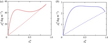
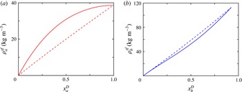
Equilibrium density of ethyl acetate (a) and butyl acetate (b) at the surface of a drop consisting of ethyl acetate and butyl acetate in water as functions of the respective mole fractions in the drop. The solid lines are the result of the theory leading to (3.5) while the dashed lines are the predictions of (4.4).

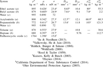
Physical properties used in the calculations. For the diffusivities we compare the experimental value, when available, with the result of (A 6); for the solubilities we compare the experimental value with the prediction of the UNIQUAC model as given by (3.7).

a Su & Needham (Reference Su and Needham2013).
b Yalkowsky, He & Jain (Reference Yalkowsky, He and Jain2010).
c Riddick, Bunger & Sakano (Reference Riddick, Bunger and Sakano1986).
d Wohlfarth (Reference Wohlfarth and Lechner2009).
e Reed & Taylor (Reference Reed and Taylor1959).
f Kaisers, Kelly & Busch (Reference Kaisers, Kelly and Busch2003).
g Haynes (Reference Haynes2014).
h California Department of Toxic Substances Control (2014).
i Ohio Environmental Protection Agency (2005).
5 Comparison with simplified theories
Before proceeding with the calculation of drop dissolution or growth, we compare the surface concentration from the theory of § 3 with the surface concentration according to the approximation (4.4) in a few cases; we avoid the last step in (4.4) using the correct value for
 $[x_{a}^{D}]_{x_{b}^{D}=0}$
rather than replacing it by 1. As noted at the end of the previous section, the approximation used by Su & Needham (Reference Su and Needham2013) is fairly close to (4.4) so that the results that we show here are representative also of those that can be obtained using (4.6).
The physical properties used in the calculations of this and the following sections are given in table 1 with appropriate references. In the case of solubilities and diffusivities we show both measured values (where available) and the values predicted by the models we use (UNIQUAC for solubilities and equation (A 6) for diffusivities) to give an idea of their validity. For the diffusivities the comparison is reasonable; we use the experimental values where available. The comparison is also good for the solubilities of the second system, while we have been unable to find experimental values for the third one. For the first system, there is a rather large difference, which indicates some problems with the values of the basic UNIQUAC model in the literature. In any event, since the focus here is to show the difference between the present and the simplified approaches, valid conclusions will be drawn provided the same numerical values are used for both.
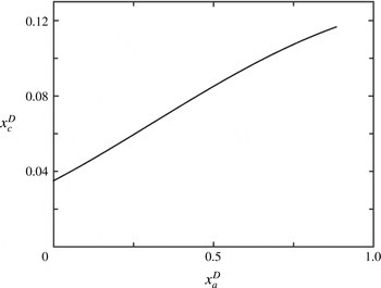
Equilibrium mole fraction of water in a drop consisting of ethyl acetate and butyl acetate as a function of the mole fraction of ethyl acetate in the drop according to the theory of § 3.

Our first example is for the system ethyl acetate (component
 $a$
), butyl acetate (component
 $b$
) in water (component
 $c$
), which is one of the cases studied by Su & Needham (Reference Su and Needham2013). Figure 1(a,b) compares the equilibrium concentrations
 ${\it\rho}_{a,b}^{sf}$
of the two organic components at the drop surface as functions of their respective mole fractions in the drop (solid lines) as given by (3.5), with the concentrations given by (4.4) (dashed lines). The lines stop at the maximum value of the mole fraction, namely
 $[x_{a}^{D}]_{x_{b}^{D}=0}$
in figure 1(a) and
 $[x_{b}^{D}]_{x_{a}^{D}=0}$
in figure 1(b). The lines do not reach 1 because the solubility of water in the organic compounds, though small, is not zero.
Equilibrium density of acrylonitrile (a) and propanenitrile (b) at the surface of a drop consisting of acrylonitrile and propanenitrile in water as functions of the respective mole fractions in the drop. The solid lines are the result of the theory leading to (3.5) while the dashed lines are the predictions of (4.4).

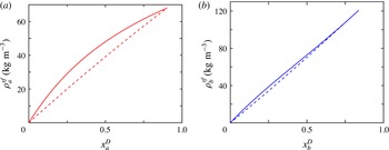
Equilibrium density of toluene (a) and heptane (b) at the surface of a drop consisting of toluene and heptane in hexadecafluorooxonane as functions of the respective mole fractions in the drop. The solid lines are the result of the theory leading to (3.5) while the dashed lines are the predictions of (4.4).

It can be seen that there is a large difference between the two sets of results, both qualitative and quantitative. In particular, there are ranges of the drop composition in which the surface concentration is not a monotonic function of the amount of that component in the drop.
The mole fraction of water in the drop is shown in figure 2 as a function of the mole fraction of ethyl acetate in the drop. It is seen to grow up to a maximum of approximately 11 % when the concentration of ethyl acetate reaches its maximum. This is a consequence of the greater solubility of water in ethyl as compared to butyl acetate.
In spite of the large differences shown in figure 1, it will be shown in § 6 (see in particular figure 7
a) that the two models give comparable results for the dissolution times of a drop consisting of these two compounds in water. The reason is that ethyl acetate has a much larger solubility in water than butyl acetate, which leads to its rapid dissolution out of the drop. The drop dissolution time is therefore mostly determined by the residual, slowly dissolving butyl acetate as shown later in figure 6(b). This is a general conclusion of our study: if the solubility or the diffusivity of a component
 $a$
is much larger than that of the other component
 $b$
, component
 $a$
will quickly dissolve away and the surface concentration of the other component will remain very close to its saturation value
 ${\it\rho}_{b}^{sat}$
for the majority of the drop lifetime. In this case, whether the precise theory of § 3 or the approximations of § 4 are used will make very little difference.
The two theories predict significant differences in drop dissolution times in the case of systems forming non-ideal solutions in which the components have comparable solubilities and comparable diffusivities in the continuous phase. One such case is that of acrylonitrile (or 2-propanenitrile,
 $\text{C}_{3}\text{H}_{3}\text{N}$
, component
 $a$
) and propanenitrile (or propionitrile,
 $\text{C}_{3}\text{H}_{5}\text{N}$
, component
 $b$
) in water (component
 $c$
). Figure 3 presents for this case information similar to that shown previously in figure 1. The surface concentration of propanenitrile as given by the two models is fairly close, while that of acrylonitrile presents differences up to approximately 25 %.
As a final example we consider a drop consisting of toluene (component
 $a$
) and heptane (component
 $b$
) in hexadecafluorooxonane (perfluorocyclic oxide,
 $\text{C}_{8}\text{F}_{16}\text{O}$
, component
 $c$
). The surface concentrations for this case are shown in figure 4. In (a) it looks as if the mole fraction of toluene ranges all the way up to 1, but in fact this is not so – this is due only to the extremely small solubility of the third component in toluene. Again, we note a substantial difference between the present more precise theory and the approximations of § 4.
6 Results for
 ${\it\rho}_{a,b}^{i}=0$

We now show some numerical results to illustrate quantitatively the consequences of the dissolution process as predicted by the present theory in some specific cases. This section is devoted to situations in which the concentration of the drop components in the host liquid is initially zero; in the next section we consider the interesting differences introduced by a non-zero initial concentration. The numerical method used to integrate the mass diffusion equation (2.4) with
 $\partial {\it\rho}_{a,b}/\partial r|_{r=R}$
given by (2.9) is described in appendix B.
As we have already remarked in § 5, conditions that lead to the strong prevalence of either one of the two main components of the drop over most of the drop lifetime will not show much difference between the present theory and (4.4) as, in this case, one deals essentially with a mono-component drop. This situation occurs, for instance, when the solubility of one of the two drop components in the host liquid is much greater than that of the other or when the diffusivities of the two components in the continuous phase are very different. Significant differences, however, are found when neither of these two conditions is satisfied. Another situation in which the two theories give significantly different results is when the initial concentration of the drop constituents in the host liquid is non-zero, as will be seen in the next section.
Since the drop constituents are only sparingly soluble in the continuous phase, we dispense with the Maxwell–Stefan theory of multicomponent diffusion (see e.g. Wesselingh & Krishna Reference Wesselingh and Krishna2000) and simply use the binary diffusivities to calculate the mass fluxes as already noted in § 2. For some substances these properties are not available; in these cases they have been estimated using (A 6) given at the end of appendix A.
Our first example is a drop composed of ethyl acetate (component
 $a$
) and butyl acetate (component
 $b$
) with an initial mole ratio of
 $n^{a}(0):n^{b}(0)=9:1$
in water and an initial drop radius of
 $43~{\rm\mu}\text{m}$
. The use of a
 $9:1$
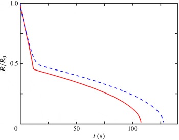
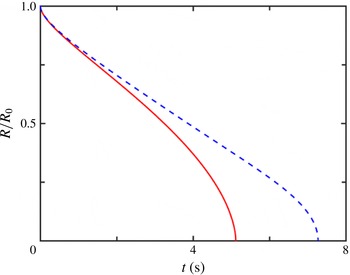
mole ratio is suggested by the fact that ethyl acetate is much more soluble in water than butyl acetate. Figure 5 compares the time dependence of the drop radius predicted by the theory of § 3 with that of the simplified model (4.4). The difference in the drop lifetime between the two models is approximately 19 s, or 15 %.
Normalized drop radius
 $R(t)/R_{0}$
versus time according to the present theory (solid line) and the model of (4.4). The drop consists of ethyl acetate (component
 $a$
) and butyl acetate (component
 $b$
) with an initial mole ratio
 $n^{a}(0):n^{b}(0)=9:1$
in water and an initial drop radius of
 $43~{\rm\mu}\text{m}$
.


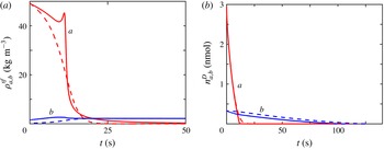
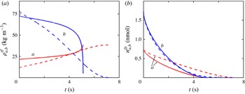
We can understand the origin of the sharp transition in these curves by looking at the history of the interface concentrations of the drop constituents shown in figure 6(a) in which, again, the solid and the dashed lines correspond to the present theory and (4.4) respectively. It is seen here that the abrupt change in the slope of the lines in figure 5 corresponds to the near complete depletion of ethyl acetate which leaves behind the much more slowly dissolving butyl acetate. The spike in the ethyl acetate concentration in figure 6(a) is due to the non-monotonic dependence of the surface concentration on the mole fractions pointed out earlier in connection with figure 1(a). The butyl acetate concentration becomes essentially constant and equal to its saturation value after the other component has dissolved away. During this latter phase the two theories predict the same surface concentration, as expected. The time dependence of the moles of the two components in the drop is shown in figure 6(b).
It is interesting to note the relatively large difference in the drop dissolution times in spite of the apparent close similarity of the predictions shown in this figure. In the precise theory the surface concentration of ethyl acetate in the initial stages of the process is higher than according to the approximate theory (see figure 6 a), which leads to a faster dissolution of this component and, ultimately, to the 15 % difference in total drop dissolution time.
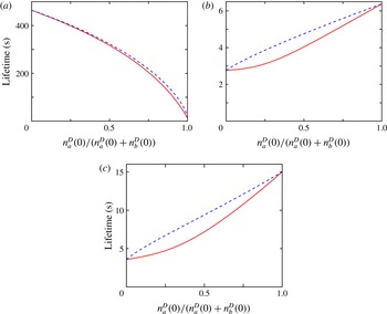
Drop lifetime according to the present theory (solid lines) and the model of (4.4) as function of the drop composition for an initial drop radius of
 $43~{\rm\mu}\text{m}$
. (a) ethyl acetate/butyl acetate/water; (b) acrylonitrile/propanenitrile/water; (c) toluene/heptane/hexadecafluorooxonane.

A summary of the drop dissolution times as functions of the drop composition for this system according to the two theories is shown in figure 7(a). Since the theories are identical for a mono-component drop, the lifetime predictions coincide at the two ends of the graphs. It is seen here that, for this particular system, differences are small for the reasons already described (although they rise to approximately 50 % when the butyl acetate is present in only trace amounts). Thus, it is not surprising that Su & Needham (Reference Su and Needham2013) concluded that their approximate model was in reasonable agreement with their experiments although the comparison between theory and experiment of their figure 5 shows a small, but systematic, over-prediction of the dissolution times in qualitative agreement with the present results. A direct comparison of the present theory with the data of Su & Needham (Reference Su and Needham2013) is not possible because, as shown in table 1 and as already noted in § 5, there is a significant difference between the solubilities predicted by UNIQUAC and the measured ones. This difference indicates that the basic version of UNIQUAC that we use is not very accurate for this particular system and a more advanced version, or a different model such as UNIFAC (see e.g. Magnussen, Rasmussen & Fredenslund Reference Magnussen, Rasmussen and Fredenslund1981), might be more suitable.
Analogous graphs for the second system considered in § 5, namely acrylonitrile and propanenitrile in water, are shown in figure 7(b), and for the third system, toluene and heptane in hexadecafluorooxonane, in (c) the initial drop diameter is, again,
 $43~{\rm\mu}\text{m}$
. It is seen here that differences for the second system can be as large as 25 % and for the third one as large as 47 %, as exemplified for an initial drop composition in the ratio
 $3:7$
of toluene to heptane in figures 8 and 9.
Figure 8 shows the large differences in the predictions for the normalized drop radius
 $R(t)/R_{0}$
versus time while figure 9 compares the predictions for the surface concentrations and moles of the two drop constituents. The rapid depletion of the more soluble heptane is predicted very similarly by both models. However, the difference between the predictions for toluene produce a large difference in the drop lifetime.
Normalized drop radius
 $R(t)/R_{0}$
versus time according to the present theory (solid line) and the model of (4.4). The drop consists of a mixture of toluene (component
 $a$
) and heptane (component
 $b$
) in hexadecafluorooxonane with an initial mole ratio
 $n^{a}(0):n^{b}(0)=3:7$
and an initial drop radius of
 $43~{\rm\mu}\text{m}$
.


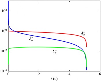
It is also of interest to study the magnitude of the three contributions accounting for the rate of diffusion of the material in the drop found by combining (2.10) and (2.4), namely
 $$\begin{eqnarray}\displaystyle & \displaystyle {\dot{A}}_{a}(t)=4{\rm\pi}R(t)D_{a}[{\it\rho}_{a}^{i}-{\it\rho}_{a}^{sf}(t)], & \displaystyle\end{eqnarray}$$
 $$\begin{eqnarray}\displaystyle & \displaystyle {\dot{B}}_{a}(t)=\frac{4{\rm\pi}R^{2}(t)D_{a}}{\sqrt{{\rm\pi}D_{a}t}}[{\it\rho}_{a}^{i}-{\it\rho}_{a}^{sf}(t)], & \displaystyle\end{eqnarray}$$
 $$\begin{eqnarray}\displaystyle & \displaystyle {\dot{C}}_{a}(t)=4{\rm\pi}R^{2}(t)D_{a}\left|\int _{0}^{t}\frac{\text{d}{\it\rho}_{a}^{sf}({\it\tau})}{\text{d}{\it\tau}}\left[\frac{1}{\sqrt{{\rm\pi}D_{a}(t-{\it\tau})}}-\frac{1}{\sqrt{{\rm\pi}D_{a}t}}\right]\text{d}{\it\tau}\right|. & \displaystyle\end{eqnarray}$$
 ${\dot{A}}_{a}(0)$
, is shown with semi-logarithmic axes in figure 10 for the toluene component of the case of figures 8 and 9; the asterisk on the symbols labelling the curves indicates that these are normalized values. The results for the other component, heptane, are similar. It is seen that the dominant term is
 ${\dot{A}}_{a}$
. The singularity in the denominator of
 ${\dot{B}}_{a}$
at
 $t=0$
causes this term to dominate for very small times, but its importance quickly decreases and the integral term
 ${\dot{C}}_{a}$
is the least important contribution. It must therefore be concluded that the major contributor to the quantitative differences found in this study is not due to this new term but, rather, to the way in which the surface concentrations are calculated.
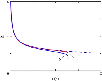
Sherwood number (defined in (6.4)) versus time for the toluene component (a) and the heptane component (b) of the toluene/heptane drop in hexadecafluorooxonane of figures 8–11 (initial mole ratio
 $n^{a}(0):n^{b}(0)=3:7$
, initial drop radius of
 $43~{\rm\mu}\text{m}$
). The results of the approximate theory (first two terms of (6.5)) nearly superpose on the dashed line.

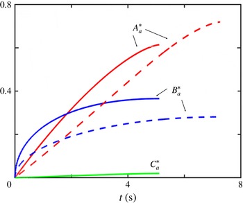
Figure 11 shows the time integrals of these three terms, namely
 $A_{a}(t)=\int _{0}^{t}{\dot{A}}_{a}({\it\tau})\,\text{d}{\it\tau}$
etc., normalized by division by
 $m_{a}(0)$
. The graphs confirm that most of the mass transfer is due to the first term
 $A_{a}(t)$
. The integral term
 $C_{a}(t)$
accounts for approximately 4 % of the total.
As a final point of interest, we show in figure 12 an example of the time dependence of the effective Sherwood numbers for the two components, defined by
 $$\begin{eqnarray}\displaystyle Sh_{a,b}=\frac{2R(t)[-\partial {\it\rho}_{a,b}/\partial r]_{r=R}}{{\it\rho}_{a,b}^{sf}(t)-{\it\rho}_{a,b}^{i}}, & & \displaystyle\end{eqnarray}$$
for the same case of figures 8–11, namely a drop composition in the ratio
 $3:7$
of toluene to heptane. By (2.10), the Sherwood number equals
 $$\begin{eqnarray}\displaystyle Sh_{a}=2+\frac{2R(t)}{\sqrt{{\rm\pi}D_{a}t}}+\frac{2R}{{\it\rho}_{a}^{sf}(t)-{\it\rho}_{a}^{i}}\int _{0}^{t}\frac{\text{d}{\it\rho}_{a}^{sf}({\it\tau})}{\text{d}{\it\tau}}\left[\frac{1}{\sqrt{{\rm\pi}D_{a}(t-{\it\tau})}}-\frac{1}{\sqrt{{\rm\pi}D_{a}t}}\right]\text{d}{\it\tau}, & & \displaystyle\end{eqnarray}$$
with a similar expression for the
 $Sh_{b}$
. The second term vanishes as
 $R\rightarrow 0$
and therefore, for the approximate model (dashed line), which does not contain the integral,
 $Sh_{a}\rightarrow 2$
. As shown in figure 9(a), however, the time derivative of the surface concentration becomes large and negative for small radius so that, for the complete model, the final value of
 $Sh_{a,b}$
dips below 2.
7 Results for
${\it\rho}_{a,b}^{i}\neq 0$

The picture described in the previous section becomes more complex when the initial concentration of the drop components in the continuous phase is non-zero. An interesting observation is that, in this case, it is possible for the ratio
 $n_{a}/n_{b}$
of the two components in the drop to take on a constant value in the early stages of the process and to maintain it until the end. This phenomenon occurs because, in view of the single degree of freedom of the system (§ 3), constancy of
 $n_{a}/n_{b}$
implies constancy of the interface concentrations. As a consequence, when
 $n_{a}/n_{b}$
has stabilized, the time dependence of the integral term in (2.10),
 $$\begin{eqnarray}\displaystyle \frac{1}{\sqrt{{\rm\pi}D_{a}t}}\int _{0}^{t}\frac{\text{d}{\it\rho}_{a}^{sf}({\it\tau})}{\text{d}{\it\tau}}\left[\frac{1}{\sqrt{1-{\it\tau}/t}}-1\right]\text{d}{\it\tau}, & & \displaystyle\end{eqnarray}$$
decreases faster than
 $t^{-1/2}$
. If the effect of this term (which anyway is small, as shown in the example of figures 10 and 11) is neglected, and if the diffusivities are not too different, with the aid of (3.2), we find from (2.4) and (2.10)
 $$\begin{eqnarray}\displaystyle \frac{\text{d}}{\text{d}t}\frac{n_{a}}{n_{b}}=\frac{M_{b}}{M_{a}}\frac{\text{d}}{\text{d}t}\frac{m_{a}}{m_{b}}\simeq \frac{4{\rm\pi}R^{2}}{M_{a}m_{b}x_{b}^{D}}\left(\frac{1}{\sqrt{{\rm\pi}D_{b}t}}+\frac{1}{R}\right){\it\Lambda}, & & \displaystyle\end{eqnarray}$$
where
 $$\begin{eqnarray}\displaystyle {\it\Lambda}=D_{a}M_{b}x_{b}^{D}({\it\rho}_{a}^{i}-{\it\rho}_{a}^{sf})-D_{b}M_{a}x_{a}^{D}({\it\rho}_{b}^{i}-{\it\rho}_{b}^{sf}). & & \displaystyle\end{eqnarray}$$
Thus,
 $(\text{d}/\text{d}t)(n_{a}/n_{b})=0$
when
 ${\it\Lambda}=0$
, i.e. when
 $$\begin{eqnarray}\displaystyle \frac{{\it\rho}_{a}^{i}-{\it\rho}_{a}^{sf}}{{\it\rho}_{b}^{i}-{\it\rho}_{b}^{sf}}=\frac{D_{b}M_{a}x_{a}^{D}}{D_{a}M_{b}x_{b}^{D}}. & & \displaystyle\end{eqnarray}$$
For given mass diffusivities and initial concentrations
 ${\it\rho}_{a,b}^{i}$
in the continuous phase, the two sides of this equation are functions of the single degree of freedom determining the equilibrium concentrations and the equality may be satisfied for specific values of that parameter. When this happens, the ratio
 $n_{a}/n_{b}=(M_{b}/M_{a})m_{a}/m_{b}$
remains constant. Clearly, this condition can only be satisfied when both
 ${\it\rho}_{a}^{i}-{\it\rho}_{a}^{sf}$
and
 ${\it\rho}_{b}^{i}-{\it\rho}_{b}^{sf}$
have the same sign, i.e. for drops which absorb or lose both components at the same time. It is important to note that, unlike binary systems,
 ${\it\rho}_{a,b}^{i}-{\it\rho}_{a,b}^{sf}$
can be positive even if the initial concentration is smaller than saturation as, when
 ${\it\rho}^{sf}$
is a monotonic function of the mole fraction (as in the majority of cases), the saturation concentration is the maximum value of
 ${\it\rho}^{sf}$
.
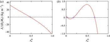
Graphs of
 ${\it\Lambda}/D_{a}M_{b}$
, with
 ${\it\Lambda}$
defined in (7.3), versus the mole fraction of toluene for the toluene/heptane/hexadecafluorooxonane system. The zeros of this quantity are the equilibrium solutions given by (7.4). They are stable when the derivative is negative and unstable otherwise. The example (a) for
 ${\it\rho}_{a}^{i}/{\it\rho}_{a}^{sat}=0.9$
,
 ${\it\rho}_{b}^{i}/{\it\rho}_{b}^{sat}=0.5$
, while that (b) for
 ${\it\rho}_{a}^{i}/{\it\rho}_{a}^{sat}=0.0026$
,
 ${\it\rho}_{b}^{i}/{\it\rho}_{b}^{sat}=0.1$
.

It is easy to see that there must always be at least one root of (7.4) and, if there are several, their number must be odd. Indeed, for
 $x_{a}^{D}=0$
,
 ${\it\Lambda}=D_{a}M_{b}(x_{b}^{D})_{max}{\it\rho}_{a}^{i}>0$
, with
 $(x_{b}^{D})_{max}$
the value of
 $x_{b}^{D}$
when
 $x_{a}^{D}=0$
. On the other hand, when
 $x_{b}^{D}=0$
,
 ${\it\Lambda}=-D_{b}M_{a}(x_{a}^{D})_{max}{\it\rho}_{b}^{i}<0$
so that the function
 ${\it\Lambda}(x_{a}^{D})$
goes through zero at least once. When there is only one root,
 $\text{d}{\it\Lambda}/\text{d}x_{a}^{D}$
evaluated at that root must be negative, which implies that the root is stable: a small increase in
 $x_{a}^{D}$
produces a negative value of
 $(\text{d}/\text{d}t)(n_{a}/n_{b})$
, which causes
 $x_{a}^{D}$
to decrease. If there is more than one root, the smallest and largest ones will be stable, while some of the intermediate ones will be unstable. The actual number of roots will depend on the initial concentrations
 ${\it\rho}_{a,b}^{i}$
in the host liquid.
Examples of the function
 ${\it\Lambda}/D_{a}M_{b}$
are shown in figure 13 for the system toluene/heptane/hexadecafluorooxonane. The example on the left is for
 ${\it\rho}_{a}^{i}/{\it\rho}_{a}^{sat}=0.9$
,
 ${\it\rho}_{b}^{i}/{\it\rho}_{b}^{sat}=0.5$
while that on the right is for
 ${\it\rho}_{a}^{i}/{\it\rho}_{a}^{sat}=0.0026$
,
 ${\it\rho}_{b}^{i}/{\it\rho}_{b}^{sat}=0.1$
. The previous arguments do not apply when either one or both
 ${\it\rho}_{a,b}^{i}$
vanish. In these cases,
 ${\it\rho}_{a}^{sf}=0$
and/or
 ${\it\rho}_{b}^{sf}=0$
may be stable or unstable equilibrium points, possibly in addition to others.
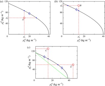
The solid lines (the same in all panels) are the surface concentration of heptane versus that of toluene for the toluene/heptane/hexadecafluorooxonane system of figure 4. The vertical dashed lines denote the values of the initial concentrations in the host liquid and a diamond marks the (single for these parameter values) equilibrium solution (7.4). The points where the curve intersects the axes correspond to the solubility of the respective component in the host liquid. The drop dissolves when the intersection point of the initial concentrations is under the curve, as in (a), while it grows when it is outside as in (b) and (c). The model (4.4) replaces the curve by the inclined straight line (green) in (c). Drops placed in a liquid with initial concentrations falling between this line and the curve are erroneously predicted to grow.

If we choose
 ${\it\rho}_{a}^{sf}$
as the single degree of freedom of the system, it is possible to plot
 ${\it\rho}_{b}^{sf}$
as a function of
 ${\it\rho}_{a}^{sf}$
; figure 14(a–c) depicts this functional dependence for the case of the toluene/heptane/hexadecafluorooxonane system of figure 4. The point where the curve intersects the horizontal axis corresponds to the solubility of component
 $a$
in the continuous phase, and similarly for the other component on the vertical axis.
Figures 14(a), 14(b) and 14(c) differ in the initial concentrations
 ${\it\rho}_{a,b}^{i}$
of the drop components in the host liquid, the values of which are indicated by the dashed horizontal and vertical lines. The points where these lines intersect are marked by the upper case letter
 $A$
in figure 14(a),
 $B$
in figure 14(b) and
 $C$
and
 $\tilde{C}$
in figure 14(c). The diamond on the curves is the only solution of (7.4) existing for the specific values of
 ${\it\rho}_{a,b}^{i}$
used in these numerical examples. From the fact that, as noted before,
 ${\it\rho}_{a}^{i}-{\it\rho}_{a}^{sf}$
and
 ${\it\rho}_{b}^{i}-{\it\rho}_{b}^{sf}$
must have the same sign at the equilibrium point, it follows that this point must lie along the arc of the curve between the intersections with the horizontal and vertical lines
 ${\it\rho}_{a}^{sf}={\it\rho}_{a}^{i}$
and
 ${\it\rho}_{b}^{sf}={\it\rho}_{b}^{i}$
.
The history of the drop growth or dissolution corresponds to the path of a point along the curves of figure 14. If there is only one equilibrium solution, it is stable and the path will be attracted by it: the growth, or dissolution, will eventually occur maintaining a constant value of
 $n_{a}(t)/n_{b}(t)$
. As noted before, unstable solutions can only occur together with stable ones. In this case, each stable point will have its own domain of attraction and the drop composition will eventually drift towards one of the stable points depending on the initial drop composition.
A consideration of the plane
 $({\it\rho}_{a}^{sf},{\it\rho}_{b}^{sf})$
also permits one to deduce when and how the drop will dissolve or grow in dependence of the initial concentrations in the continuous phase. Consider, for example, figure 14(a) and suppose that the initial drop composition is such that the surface concentration (which must be on the
 $({\it\rho}_{a}^{sf},{\it\rho}_{b}^{sf})$
curve for equilibrium) is near the lower right corner, so that
 ${\it\rho}_{a}^{sf}(t=0)>{\it\rho}_{a}^{i}$
while
 ${\it\rho}_{b}^{sf}(t=0)<{\it\rho}_{b}^{i}$
. It is evident from (2.10) that component
 $a$
will start to diffuse out of the drop while component
 $b$
will diffuse in so that the drop composition moves up the curve until it eventually reaches the equilibrium point marked by a diamond in the figure. At this point
 ${\it\rho}_{a}^{sf}$
and
 ${\it\rho}_{b}^{sf}$
exceed
 ${\it\rho}_{a}^{i}$
and
 ${\it\rho}_{b}^{i}$
and both components will diffuse out so that the drop ultimately shrinks to zero radius.
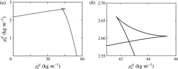
Surface concentration of butyl acetate versus that of ethyl acetate for the system ethyl acetate/butyl acetate/water. As shown in figure 1(a,b), in this case the dependence of the surface concentrations on the drop composition is non-monotonic and this feature is responsible for the small loop in (a) which is enlarged in (b).

Arguments of this type lead to the conclusion that, when the intersection of the two lines
 $({\it\rho}_{a}^{i},{\it\rho}_{b}^{i})$
lies under the curve, both constituents of the drop ultimately diffuse out and the drop dissolves, and conversely when the intersection point lies outside the curve. When the host liquid is supersaturated with one or both components, as in points
 $C$
and
 $\tilde{C}$
in figure 14(c), the drop grows as would be expected even without analysis. However, it will be noticed that it is possible for growth to occur even in a host liquid undersaturated with both components of the drop as indicated by the point
 $B$
in figure 14(b). This is impossible in a binary system, but it becomes possible in a ternary or higher-order system.
The approximate model of (4.4) replaces the curves in figure 14 by the inclined straight line (green) shown in (c). Drops placed in a liquid with initial concentrations falling between this line and the curve are erroneously predicted to grow.
These general conclusions may be expected to hold also for a non-spherical drop such as, for example, a drop sinking or rising by buoyancy, provided that the drop composition remains homogeneous, the two diffusivities in the host liquid are not too different and history effects are negligible, as we have assumed. Indeed, by the linearity of the diffusion equation, in these more general cases the rate of change of the moles of each component must be proportional to
 $D_{a,b}({\it\rho}_{a,b}^{i}-{\it\rho}_{a,b}^{sf})/M_{a,b}$
, which is the only feature of the specific solution for a stationary drop that we have used in the previous argument.
The situation depicted in figure 14 is typical of systems in which the surface concentration of each component is a monotonic function of the corresponding mole fraction. The case in which the dependence of the surface concentrations on the mole fractions is non-monotonic, as in the case of figure 1(a), is more complex, although the equilibrium points and their stability can be studied numerically similarly to figure 13. The dependence of
 ${\it\rho}_{b}^{sf}$
on
 ${\it\rho}_{a}^{sf}$
for the ethyl acetate/butyl acetate/water system is shown in figure 15. The small loop in (a) (magnified in (b)) is due to the presence of the maxima in the curves of figure 1(a,b).
8 Summary and conclusions
We have presented a consistent theory for the dissolution, or growth, of a multi-component, well-mixed spherical drop at rest in a host liquid. The theory incorporates in a proper way the constraints of thermodynamic equilibrium at the drop surface by the adoption of UNIQUAC, a widely used model for the parametrization of the activity coefficients of many chemical compounds.
The gradual change of the drop composition due to the different solubilities and diffusivities of its components in the host liquid causes a variation in time of the concentration of these components at the surface of the drop. This circumstance requires a modification of the classic theory of Epstein & Plesset (Reference Epstein and Plesset1950), which introduces memory effects in the diffusive flux out of the drop as shown in (2.9).
For the case in which the drop constituents are already present in the host liquid at the beginning of the process, we have found that, whatever the initial composition, the mole ratio of the drop constituents will reach a steady constant value for both dissolution and growth. We have formulated a simple criterion to predict whether one or the other will take place in any specific situation. In suitable conditions, a drop can grow even when the concentration of both constituents in the host liquid is smaller than their respective saturation values. This observation can have significant implications for solvent extraction processes which are widely used in the chemical and environmental remediation industries.
The predictions of the theory have been compared with those of a simpler approach to the problem built on the assumption of independence of the activity coefficients from the drop composition. It is found that the predictions of the two theories are similar when the solutions are close to ideal or there is a large difference in the solubilities, or diffusivities, of the drop constituents in the host liquid, unless initially the drop consists mainly of the more soluble component. When the solubilities and diffusivities are close, the differences can be substantial for any drop composition. Thus, an experimental confirmation of our results would require the use of liquids forming non-ideal solutions and having comparable solubilities and diffusivities in the host liquid. Furthermore, the drop should be small enough that the diffusion time of its constituents is smaller than the dissolution time so as to ensure spatial uniformity of its composition.
To the extent that the drop considered in this work is spherical and homogeneous, with no relative motion with respect to the host liquid, our model is idealized. However, in § 7, we have presented arguments to show that these conclusions are valid beyond the limits of the model, e.g. for a sessile or translating drop.
Although in this paper we have only considered the ternary system, the same general approach would apply more broadly to systems with more than three components. In particular, quaternary systems can be studied by the same method, as the UNIQUAC model is known to give reasonable results for many such systems (see e.g. Chen et al. Reference Chen, Wen, Zhou and Zeng2014).
Acknowledgements
The authors express their gratitude to an anonymous referee who made several useful suggestions. A.P. wishes to thank Dr D. Lohse for introducing him to the problem and to the work of Needham and collaborators, and for several discussions on the topic of this paper. The study was made possible by a grant from BP/The Gulf of Mexico Research Initiative through the University of Texas Marine Science Institute (DROPPS consortium: ‘Dispersion Research on Oil: Physics and Plankton Studies’). The funders had no role in the study design, data collection and analysis, decision to publish, or preparation of the manuscript.
Appendix A. The UNIQUAC model
There are several versions of the UNIQUAC model (see e.g. Taylor & Krishna Reference Taylor and Krishna1993; Tamura et al. Reference Tamura, Chen, Tada, Yamada and Nagata2000; Islam, Javvadi & Kabadi Reference Islam, Javvadi and Kabadi2011) but, for the purposes of this paper, the basic formulation of Abrams & Prausnitz (Reference Abrams and Prausnitz1975) and Anderson & Prausnitz (Reference Anderson and Prausnitz1978a ,Reference Anderson and Prausnitz b ) is sufficient.
The activity coefficient
 ${\it\gamma}_{a}$
of a component
 $a$
is expressed as the product of a combinatorial contribution
 ${\it\gamma}_{a}^{c}$
and a residual contribution
 ${\it\gamma}_{a}^{r}$
,
 ${\it\gamma}_{a}={\it\gamma}_{a}^{c}{\it\gamma}_{a}^{r}$
. The combinatorial term is given by
 $$\begin{eqnarray}\displaystyle \log {\it\gamma}_{a}^{c}=1-\frac{{\it\Phi}_{a}}{x_{a}}+\log \frac{{\it\Phi}_{a}}{x_{a}}-\frac{1}{2}zq_{a}\left(1-\frac{{\it\Phi}_{a}}{{\it\theta}_{a}}+\log \frac{{\it\Phi}_{a}}{{\it\theta}_{a}}\right). & & \displaystyle\end{eqnarray}$$
Here
 ${\it\Phi}_{a}$
is the volume fraction of the
 $a$
-component:
 $$\begin{eqnarray}\displaystyle {\it\Phi}_{a}=\frac{x_{a}r_{a}}{x_{a}r_{a}+x_{b}r_{b}+x_{c}r_{c}}, & & \displaystyle\end{eqnarray}$$
with
 $r$
’s model parameter related to the molecular volumes of each substance. The quantity
 ${\it\theta}_{a}$
is the area fraction of the component expressed in a similar way:
 $$\begin{eqnarray}\displaystyle {\it\theta}_{a}=\frac{x_{a}q_{a}}{x_{a}q_{a}+x_{b}q_{b}+x_{c}q_{c}}, & & \displaystyle\end{eqnarray}$$
with the parameters
 $q$
other pure-component molecular structure constants. The residual contribution is expressed as
 $$\begin{eqnarray}\displaystyle {\it\gamma}_{a}^{r}=q_{a}\left(1-\log \frac{\displaystyle \mathop{\sum }_{k}q_{k}x_{k}{\it\tau}_{ka}}{\displaystyle \mathop{\sum }_{k}q_{k}x_{k}}-\mathop{\sum }_{k}\frac{q_{k}x_{k}{\it\tau}_{ak}}{\displaystyle \mathop{\sum }_{\ell }q_{\ell }x_{\ell }{\it\tau}_{\ell k}}\right), & & \displaystyle\end{eqnarray}$$
in which the summations are over the three components
 $a$
,
 $b$
and
 $c$
. The quantities
 ${\it\tau}_{k\ell }$
are expressed as
 $$\begin{eqnarray}\displaystyle \log {\it\tau}_{k\ell }=-\frac{A_{k\ell }}{T}, & & \displaystyle\end{eqnarray}$$
in which the
 $A$
are binary interaction parameters. The coordination number
 $z$
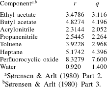
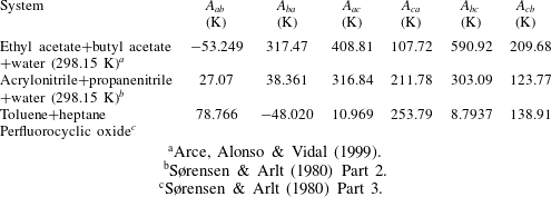
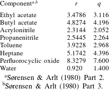
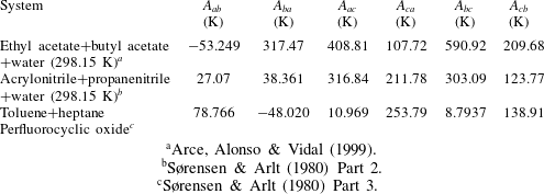
in (A 1) is taken equal to 10. The values of the other model parameters are given in tables 2 and 3 for all the compounds used in the numerical examples given in this paper. The numerical calculation of the liquid–liquid equilibrium line was effected using the method of Prausnitz et al. (Reference Prausnitz, Anderson, Grens, Eckert, Hsieh and O’Connell1980) and Islam, Zavvadi & Kabadi (Reference Islam, Zavvadi and Kabadi2012).
Values of the parameters
 $r$
and
 $q$
of the UNIQUAC model used in this work.
Values of the binary interaction parameters
 $A$
used in (A 5) of the UNIQUAC model used in this work.
For some liquids we have been unable to find values of the binary diffusivities in the continuous phase. In these cases we have used the following empirical relation giving the diffusivity of solute
 $A$
in solvent
 $B$
(Poling, Prausnitz & O’Connell Reference Poling, Prausnitz and O’Connell2000):
 $$\begin{eqnarray}\displaystyle D_{AB}=1.55\times 10^{-8}\frac{V_{B}^{0.87}}{V_{A}^{0.42}}\frac{T^{1.29}}{{\it\mu}_{B}^{0.92}}\frac{{\it\sigma}_{B}^{0.125}}{{\it\sigma}_{A}^{0.105}}. & & \displaystyle\end{eqnarray}$$
Here
 $V$
denotes the molar volume in
 $\text{g}~\text{mol}^{-1}$
,
 $T$
the absolute temperature in Kelvins,
 ${\it\mu}$
the viscosity in mPa s and
 ${\it\sigma}$
the surface tension in
 $\text{mN}~\text{m}^{-1}$
.
Appendix B. Numerical method
The equation to be solved is
 $$\begin{eqnarray}\displaystyle \frac{\text{d}m_{a}}{\text{d}t}=4{\rm\pi}R^{2}(t)D_{a}\left[\frac{{\it\rho}_{a}^{i}-{\it\rho}_{a}^{sf}(0)}{\sqrt{{\rm\pi}D_{a}t}}+\frac{{\it\rho}_{a}^{i}-{\it\rho}_{a}^{sf}(t)}{R}-\int _{0}^{t}\frac{\text{d}{\it\rho}_{a}^{sf}({\it\tau})}{\text{d}{\it\tau}}\frac{\text{d}{\it\tau}}{\sqrt{{\rm\pi}D_{a}(t-{\it\tau})}}\right]. & & \displaystyle\end{eqnarray}$$
To deal with the singularity of the integrand we approximate the integral as
 $$\begin{eqnarray}\displaystyle & & \displaystyle \int _{0}^{t^{n+1}}\frac{{\it\rho}_{a}^{sf}({\it\tau})}{\text{d}{\it\tau}}\frac{\text{d}{\it\tau}}{\sqrt{{\rm\pi}D_{a}(t^{n+1}-{\it\tau})}}\simeq \int _{0}^{t^{n}}\frac{\text{d}{\it\rho}_{a}^{sf}({\it\tau})}{\text{d}{\it\tau}}\frac{\text{d}{\it\tau}}{\sqrt{{\rm\pi}D_{a}(t^{n+1}-{\it\tau})}}\nonumber\\ \displaystyle & & \displaystyle \qquad +\,\frac{1}{\sqrt{{\rm\pi}D_{a}}}\left[\frac{\text{d}{\it\rho}_{a}^{sf}}{\text{d}t}\right]_{t^{n+1}}\int _{t^{n}}^{t^{n+1}}\frac{\text{d}{\it\tau}}{\sqrt{{\rm\pi}D_{a}(t^{n+1}-{\it\tau})}}\nonumber\\ \displaystyle & & \displaystyle \quad =\int _{0}^{t^{n}}\frac{\text{d}{\it\rho}_{a}^{sf}({\it\tau})}{\text{d}{\it\tau}}\frac{\text{d}{\it\tau}}{\sqrt{{\rm\pi}D_{a}(t^{n+1}-{\it\tau})}}+2\sqrt{\frac{t^{n+1}-t^{n}}{{\rm\pi}D_{a}}}\left[\frac{\text{d}{\it\rho}_{a}^{sf}}{\text{d}t}\right]_{t^{n+1}}.\end{eqnarray}$$
The derivative in the last term is evaluated at the same time level as
 $\text{d}m_{a}/\text{d}t$
in the left-hand side of (B 1), which confers to the procedure a desirable degree of implicitness. For completeness we now describe the remaining steps of the calculation.
From (3.5) we write
 $\text{d}{\it\rho}_{a}^{sf}/\text{d}t\equiv \dot{{\it\rho}}_{a}^{sf}$
in the form
 $$\begin{eqnarray}\displaystyle \dot{{\it\rho}}_{a}^{sf}={\dot{x}}_{a}^{D}\frac{\text{d}}{\text{d}x_{a}^{D}}\left(\frac{M_{a}x_{a}^{C}}{M_{c}x_{c}^{C}}{\it\rho}_{c}^{0}\right), & & \displaystyle\end{eqnarray}$$
with a similar equation for
 $\dot{{\it\rho}}_{b}^{sf}$
obtained by interchanging the indices
 $a$
and
 $b$
. The derivative of the quantity in parentheses is calculated numerically due to the very complex functional dependence of the quantities involved upon
 $x_{a}^{D}$
. The derivative
 ${\dot{x}}_{a}^{D}$
is then expressed in terms of
 ${\dot{m}}_{a}$
and
 ${\dot{m}}_{b}$
by using the relation of this quantity with the auxiliary parameter
 $\tilde{x}_{a}^{D}=(m_{a}/M_{a})/(m_{a}/M_{a}+m_{b}/M_{b})$
. This step expresses
 $\dot{{\it\rho}}_{a}^{sf}$
in terms of a linear combination of
 ${\dot{m}}_{a}$
and
 ${\dot{m}}_{b}$
, and a relation with a similar structure is obtained for
 $\dot{{\it\rho}}_{b}^{sf}$
. Upon substitution into the last term of (B 2) and the analogous relation for the other component we are left with a linear system of two equations in the two unknowns
 ${\dot{m}}_{a}$
and
 ${\dot{m}}_{b}$
which can be readily solved and integrated.
To execute the first time step, which is affected by the singularity at
 $t=0$
in the first term in the right-hand side of (B 1), we use the approximation
 $$\begin{eqnarray}\displaystyle \int _{0}^{{\rm\Delta}t_{1}}4{\rm\pi}R^{2}(t)D_{a}\frac{{\it\rho}_{a}^{i}-{\it\rho}_{a}^{sf}(0)}{\sqrt{{\rm\pi}D_{a}t}}\,\text{d}t\simeq 8{\rm\pi}R^{2}(0)D_{a}[{\it\rho}_{a}^{i}-{\it\rho}_{a}^{sf}(0)]\sqrt{\frac{{\rm\Delta}t_{1}}{{\rm\pi}D_{a}}}, & & \displaystyle\end{eqnarray}$$
where
 ${\rm\Delta}t_{1}$
is the first time step. At this point the procedure previously described can be started. As a rough check we have used different values for
 ${\rm\Delta}t_{1}$
finding that the results at later times were essentially unaffected.