1 Introduction
The oscillatory motion of Lagrangian particles below surface gravity waves is subject to a net drift in the direction of wave propagation known as Stokes drift (Stokes Reference Stokes1847). For wave groups, the net positive transport associated with the Stokes drift becomes divergent on the group scale and is accompanied by an opposing Eulerian return flow (Longuet-Higgins & Stewart Reference Longuet-Higgins and Stewart1962). The total Lagrangian velocity is given by the sum of the Stokes drift and the induced Eulerian flow, and the resulting particle trajectories and displacements have been examined theoretically by van den Bremer & Taylor (Reference van den Bremer and Taylor2015, Reference van den Bremer and Taylor2016).
In the ocean, Stokes drift can provide a significant contribution to the trajectories of drifters (Röhrs et al. Reference Röhrs, Christensen, Hole, Broström, Drivdal and Sundby2012) and must be accounted for in search and recovery missions such as the search for debris from the presumed location of the 2014 MH370 airplane crash (Trinanes et al. Reference Trinanes, Olascoaga, Goni, Maximenko, Griffin and Hafner2016). Stokes drift can be important in the local modelling of oil spills (Christensen & Terrile Reference Christensen and Terrile2009; Drivdal, Broström & Christensen Reference Drivdal, Broström and Christensen2014; Jones et al. Reference Jones, Dagestad, Breivik, Holt, Röhrshrs, Christensen, Espeseth, Brekke and Skrunes2016). In the near-surface transport and dispersion of plastic pollution, Stokes drift plays a potentially important yet largely unexplored role (e.g. Lebreton et al. Reference Lebreton, Slat, Ferrari, Sainte-Rose, Aitken, Marthouse, Hajbane, Cunsolo, Schwarz and Levivier2018). Furthermore, Stokes drift is considered a mechanism driving global ocean circulation (McWilliams & Restrepo Reference McWilliams and Restrepo1999; Belcher et al. Reference Belcher, Grant, Hanley, Fox-Kemper, Roekel, Sullivan, Large, Andy, Hines and Calvert2012), Langmuir turbulence (Craik & Leibovich Reference Craik and Leibovich1976; Sullivan & McWilliams Reference Sullivan and McWilliams2010; D’Asaro et al. Reference D’Asaro, Thomson, Shcherbina, Harcourt, Cronin, Hemer and Fox-Kemper2014) and sub-mesoscale ocean instability (Haney et al. Reference Haney, Fox-Kemper, Julien and Webb2015; McWilliams Reference McWilliams2016).
Experimentally, many authors have considered Stokes drift in laboratory wave flumes. As a visual illustration, Wallet & Ruellan’s (1950) seminal image of orbits that do not quite close is reproduced in Van Dyke’s (Reference Van Dyke1982) Album of Fluid Motion. Yet, there remains some confusion in the literature about whether a net drift should be observed (see the discussion in Monismith et al. (Reference Monismith, Cowen, Nepf, Magnaudet and Thais2007), Weber (Reference Weber2011), Grue & Kolaas (Reference Grue and Kolaas2017), van den Bremer & Breivik (Reference van den Bremer and Breivik2017) and Deike, Pizzo & Melville (Reference Deike, Pizzo and Melville2017)). To explain this, three effects must be taken into account: boundary layers, the origin of vorticity in the interior of the fluid and breaking.
Longuet-Higgins (Reference Longuet-Higgins1953) showed that the mass-transport velocity can be significantly different from the irrotational theory of Stokes (Reference Stokes1847), with additional net transport arising in the oscillating bottom and surface boundary layers. Explaining experiments by Bagnold (Reference Bagnold1947), Longuet-Higgins (Reference Longuet-Higgins1953) showed that the Lagrangian transport in the boundary layers is positive and does not disappear in the limit of infinite Reynolds number. This boundary layer streaming has recently been studied for very steep waves by Grue & Kolaas (Reference Grue and Kolaas2017), who observed significant additional streaming and associated shear in both the bottom and free surface boundary layers, more than can be predicted by the boundary layer streaming solution of Longuet-Higgins (Reference Longuet-Higgins1953), which Grue & Kolaas (Reference Grue and Kolaas2017) noted may be invalid owing to the large steepness of the waves.
For periodic waves, which are the focus of almost all experimental studies focusing on wave-induced mean flows, the net depth-integrated mass flux must be zero in a closed flume. The Stokes transport must be accompanied by a Eulerian return current driven by a set-up in the direction downstream of wave propagation, which is conceptually distinct from the return flow forced by the packet structure examined herein. This closed-flume return flow is irrotational, unless vorticity can be transported into the interior of the fluid. Longuet-Higgins (Reference Longuet-Higgins1953) derived two classes of analytical solutions for this vorticity transport: a ‘conduction’ solution and a ‘convection’ solution. Depending on the ratio of the wave amplitude
 $a$
to the thickness of the boundary layer
 $\unicode[STIX]{x1D6FF}$
, the transport of vorticity takes place by viscous ‘conduction’ (
 $a^{2}/\unicode[STIX]{x1D6FF}^{2}$
small) from the bottom and free surface boundary layers, or convection with the mass-transport velocity (
 $a^{2}/\unicode[STIX]{x1D6FF}^{2}$
large), from the wavemaker or the beach at the other end, where vorticity can be generated. If one considers a motion that is started from rest, the motion in the interior of the fluid will always be initially irrotational, and it will take considerable time for vorticity to be advected or diffused from the vertical or horizontal boundaries, respectively. Finally, as also pointed out by Longuet-Higgins (Reference Longuet-Higgins1953), the convection solution may not be stable.
In the conduction regime, Groeneweg & Klopman (Reference Groeneweg and Klopman1998) compare their more generally applicable generalized Lagrangian mean model for wave–current interaction to the conduction solution of Longuet-Higgins (Reference Longuet-Higgins1953), showing near perfect agreement, and to the laboratory measurements in a very shallow and long closed flume by Mei, Liu & Carter (Reference Mei, Liu and Carter1972), finding good agreement for intermediate water depth (
 $kd=1.0$
, with
 $k$
the wavenumber and
 $d$
the water depth), but less good agreement for deeper water (
 $kd=1.8$
). However, most experimental studies are in the convection regime. Swan (Reference Swan1990) demonstrated that convection indeed plays an important part within a relatively deep experimental wave flume: vorticity generated at the end conditions is convected backwards with the mass transport velocity and the near-shore region progressively influences the entire length of the wave flume, although the flow field is not always stable. By installing a plastic sheet at the toe of the beach, Swan & Sleath (Reference Swan and Sleath1990) could obtain long-time stable conditions that agreed better with their fourth-order finite-depth extension of the irrotational solution for Lagrangian transport in a closed domain. Umeyama (Reference Umeyama2012) performed a similar expansion, but focused explicitly on particle trajectories and found reasonable agreement with experimentally obtained trajectories. Paprota, Sulisz & Reda (Reference Paprota, Sulisz and Reda2016), who took their measurements after a relatively short wave train of periodic waves in a relatively long flume, found good agreement with the irrotational theory of Stokes (Reference Stokes1847), supplemented by a closed-flume return current. For waves of intermediate water depth (
 $kd=O(1)$
) and very large steepness, Grue & Kolaas (Reference Grue and Kolaas2017) found good agreement with nonlinear irrotational theory in the interior of the fluid in a set of very high-quality experiments. Their experiments were stopped long before the first waves reached the end of their open-ended flume, but the length of their wave train remained long relative to the water depth. Based on their experiments, Monismith et al. (Reference Monismith, Cowen, Nepf, Magnaudet and Thais2007) have suggested a cancellation of the Stokes drift by a Eulerian mean flow that is equal and opposite at every depth. Their experiments were done in the presence of a pre-existing sheared current in a recirculating flume, which could help explain their observation. The current could also advect vorticity at a faster rate than the wave-induced mean flow.
If the waves are breaking, transport of Lagrangian particles near the surface will be considerably enhanced, as observed experimentally by Melville & Rapp (Reference Melville and Rapp1988) and recently explained using numerical simulations and a scaling argument for breaking by Deike et al. (Reference Deike, Pizzo and Melville2017) with implications for surfing (Pizzo Reference Pizzo2017). Breaking also has the capacity to transport vorticity into the interior of the fluid (Pizzo & Melville Reference Pizzo and Melville2013).
This paper presents an experimental study of Lagrangian trajectories and transport by uni-directional deep-water small-amplitude short-length yet quasi-monochromatic surface gravity wave groups. In doing so, we visualize experimentally for the first time the wave-induced Eulerian return flow for groups. We also show that our experimental observations in this regime are in good agreement with leading-order solutions to the irrotational water wave equations. Our experiments using short-length groups in an otherwise quiescent flume have the advantage of not generating a closed-flume return flow, which may transport vorticity, is potentially unstable and difficult to control experimentally.
Furthermore, our experiments demonstrate the existence of a vertical component to the Stokes drift, which only exists for wave groups and results in a positive (temporary) vertical particle displacement underneath the centre of the group. This positive vertical displacement by the Stokes drift has been predicted by Herbers & Janssen (Reference Herbers and Janssen2016), who showed that the set-down of the wave-averaged free surface in Eulerian records can appear as (significant) set-up in Lagrangian (buoy) records. Nevertheless, a vertical component to the Stokes drift (for groups) has been contentious in adaptations of the work by Craik & Leibovich (Reference Craik and Leibovich1976) in the context of ocean circulation and Langmuir circulation. McWilliams, Restrepo & Lane (Reference McWilliams, Restrepo and Lane2004) noted that the vertical Stokes drift is zero and introduced a vertically divergent vertical pseudo-velocity to compensate for the horizontal divergence of the Stokes drift. Although Mellor (Reference Mellor2016) allows for a horizontally divergent Stokes drift, he still requires the vertical Stokes drift component to be zero. We emphasize that the Stokes drift velocity is generally divergent for groups; this is consistent with generalized Lagrangian-mean theory (Andrews & McIntyre Reference Andrews and McIntyre1978), as shown by McIntyre (Reference McIntyre1988). Accordingly, a vertical Stokes drift component arises for groups, as can be easily derived for irrotational surface gravity waves and is confirmed experimentally herein.
This paper is laid out as follows. First, § 2 briefly summarizes the irrotational solutions for wave groups, followed by a description of our experimental methodology in § 3. We present results in § 4, including illustrations of the Lagrangian orbits, a comparison with irrotational water wave theory and an assessment of the experimental error, and draw conclusions in § 5.
2 Irrotational water wave theory for wave groups
2.1 Governing equations and leading-order solutions
In a two-dimensional body of water of depth
 $d$
with coordinate system (
 $x$
,
 $z$
) and
 $z$
the vertical coordinate measured from the undisturbed water level upwards, inviscid, incompressible and irrotational flow leads to Laplace
 $\unicode[STIX]{x1D6FB}^{2}\unicode[STIX]{x1D719}=0$
for
 $-d\leqslant z\leqslant \unicode[STIX]{x1D702}(x,t)$
as the governing equation, where the velocity vector
 $\boldsymbol{u}=\unicode[STIX]{x1D735}\unicode[STIX]{x1D719}$
and
 $\unicode[STIX]{x1D702}(x,t)$
denotes the free surface. By retaining terms up to quadratic in the amplitude of the waves, the kinematic free surface boundary condition (
 $w-\unicode[STIX]{x2202}\unicode[STIX]{x1D702}/\unicode[STIX]{x2202}t-u\unicode[STIX]{x2202}\unicode[STIX]{x1D702}/\unicode[STIX]{x2202}x=0$
) and the dynamic free surface boundary condition (
 $g\unicode[STIX]{x1D702}+\unicode[STIX]{x2202}\unicode[STIX]{x1D719}/\unicode[STIX]{x2202}t+(u^{2}+w^{2})/2=0$
), both at
 $z=\unicode[STIX]{x1D702}(x,t)$
, can be combined into two forcing equations for the mean flow and the wave-averaged free surface, respectively (e.g. Longuet-Higgins & Stewart Reference Longuet-Higgins and Stewart1964; McAllister et al.
Reference McAllister, Adcock, Taylor and van den Bremer2018):
 $$\begin{eqnarray}\displaystyle \left({\displaystyle \frac{\unicode[STIX]{x2202}}{\unicode[STIX]{x2202}z}}\left.+{\displaystyle \frac{1}{g}}{\displaystyle \frac{\unicode[STIX]{x2202}^{2}}{\unicode[STIX]{x2202}t^{2}}}\right)\unicode[STIX]{x1D719}^{(2)}\right|_{z=0}=\overline{{\displaystyle \frac{\unicode[STIX]{x2202}}{\unicode[STIX]{x2202}x}}(u^{(1)}|_{z=0}\unicode[STIX]{x1D702}^{(1)})}+O(\unicode[STIX]{x1D6FC}^{2}\unicode[STIX]{x1D716}^{3}),\quad \unicode[STIX]{x1D702}^{(2)}={\displaystyle \frac{-1}{g}}\left.{\displaystyle \frac{\unicode[STIX]{x2202}\unicode[STIX]{x1D719}^{(2)}}{\unicode[STIX]{x2202}t}}\right|_{z=0}+O(\unicode[STIX]{x1D6FC}^{2}\unicode[STIX]{x1D716}^{3}),\hspace{-12.0pt} & & \displaystyle \nonumber\\ \displaystyle & & \displaystyle\end{eqnarray}$$
where the superscripts denote the order in amplitude, and we only retain wave-averaged terms here, as indicated by the overlines on the right-hand side of (2.1a
). The small parameter corresponding to amplitude, steepness, is denoted by
 $\unicode[STIX]{x1D6FC}\equiv k_{0}|a_{0}|$
, where
 $a_{0}$
is the typical amplitude of the surface elevation and
 $k_{0}$
the wavenumber of the carrier wave. Explicitly, we thus have for the Stokes expansion in
 $\unicode[STIX]{x1D6FC}$
that
 $\unicode[STIX]{x1D719}=\unicode[STIX]{x1D719}^{(1)}+\unicode[STIX]{x1D719}^{(2)}+O(\unicode[STIX]{x1D6FC}^{3})$
and
 $\unicode[STIX]{x1D702}=\unicode[STIX]{x1D702}^{(1)}+\unicode[STIX]{x1D702}^{(2)}+O(\unicode[STIX]{x1D6FC}^{3})$
, where we will only retain the wave-averaged terms in
 $\unicode[STIX]{x1D719}^{(2)}$
and
 $\unicode[STIX]{x1D702}^{(2)}$
. In (2.1) we have made the additional assumption that
 $k_{0}d\gg 1$
, so that the set-down of the wave-averaged free surface
 $\unicode[STIX]{x1D702}^{(2)}$
does not directly affect the mean flow (McIntyre Reference McIntyre1981; McAllister et al.
Reference McAllister, Adcock, Taylor and van den Bremer2018). More specifically, we set
 $\unicode[STIX]{x1D702}^{(1)}=\text{Re}[A_{0}(X)\exp (\text{i}(k_{0}x-\unicode[STIX]{x1D714}_{0}t))+\unicode[STIX]{x1D716}A_{1}(X)\exp (\text{i}(k_{0}x-\unicode[STIX]{x1D714}_{0}t))]$
and
 $\unicode[STIX]{x1D719}^{(1)}=\text{Re}[B_{0}\exp (k_{0}z+\text{i}(k_{0}x-\unicode[STIX]{x1D714}_{0}t))+\unicode[STIX]{x1D716}B_{1}\exp (k_{0}z+\text{i}(k_{0}x-\unicode[STIX]{x1D714}_{0}t))]$
, where
 $X\equiv \unicode[STIX]{x1D716}(x-c_{g,0}t)$
with
 $\unicode[STIX]{x1D716}\equiv 1/(k_{0}\unicode[STIX]{x1D70E})$
,
 $\unicode[STIX]{x1D70E}$
the characteristic length of the group and
 $c_{g,0}=\text{d}\unicode[STIX]{x1D714}_{0}/\text{d}k_{0}=\unicode[STIX]{x1D714}_{0}/(2k_{0})$
the group velocity. The linear (
 $O(\unicode[STIX]{x1D6FC})$
) polarization relationships at the zeroth and first order in
 $\unicode[STIX]{x1D716}$
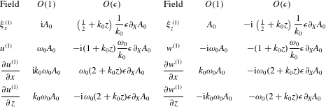
are given in table 1.
Expressions for the different linear (in
 $\unicode[STIX]{x1D6FC}\equiv k_{0}|a_{0}|$
) fields at
 $O(\unicode[STIX]{x1D6FC}^{1}\unicode[STIX]{x1D716}^{0})$
and
 $O(\unicode[STIX]{x1D6FC}^{1}\unicode[STIX]{x1D716}^{1})$
. Values are given in terms of the leading-order amplitude envelope
 $A_{0}$
of the vertical displacement field. The actual fields are the real parts of the tabulated expressions after multiplication by
 $\exp (k_{0}z+\text{i}\unicode[STIX]{x1D711}_{0})$
, where the phase is given by
 $\unicode[STIX]{x1D711}_{0}=k_{0}x-\unicode[STIX]{x1D714}_{0}t$
. We denote
 $\unicode[STIX]{x1D702}^{(1)}\equiv \unicode[STIX]{x1D709}_{z}^{(1)}(z=0)$
as the free surface.

Our focus is on leading-order terms; we ignore dispersion of the group (e.g. van den Bremer & Taylor Reference van den Bremer and Taylor2016), and the second-order equations in steepness (2.1) are accurate up to
 $O(\unicode[STIX]{x1D716}^{3})$
in the bandwidth parameter
 $\unicode[STIX]{x1D716}$
, as can be shown from the linear polarization relationships in table 1. The leading-order non-dispersive mean flow solution is given by combining the linear polarization relationships in table 1 and solving Laplace
 $\unicode[STIX]{x1D6FB}^{2}\unicode[STIX]{x1D719}^{(2)}=0$
subject to the bottom boundary condition
 $\unicode[STIX]{x2202}\unicode[STIX]{x1D719}^{(2)}/\unicode[STIX]{x2202}z=0$
at
 $z=-d$
and the surface forcing (2.1a
) (see also van den Bremer & Taylor (Reference van den Bremer and Taylor2016))
 $$\begin{eqnarray}\displaystyle \unicode[STIX]{x1D719}_{E}^{(2)}={\displaystyle \frac{-\unicode[STIX]{x1D714}_{0}}{4\unicode[STIX]{x03C0}}}\displaystyle \int _{-\infty }^{\infty }{\displaystyle \frac{\cosh (|\unicode[STIX]{x1D714}|(z+d)/c_{g,0})}{\sinh (|\unicode[STIX]{x1D714}|d/c_{g,0})}}{\displaystyle \frac{\unicode[STIX]{x1D714}}{|\unicode[STIX]{x1D714}|}}{\displaystyle \frac{\text{i}\widehat{|A_{0}|^{2}}}{1-{\displaystyle \frac{\unicode[STIX]{x1D714}^{2}c_{g,0}}{g|\unicode[STIX]{x1D714}|\tanh (|\unicode[STIX]{x1D714}|d/c_{g,0})}}}}\exp (\text{i}\unicode[STIX]{x1D714}\tilde{t})\,\text{d}\unicode[STIX]{x1D714},\quad & & \displaystyle\end{eqnarray}$$
where we choose
 $c_{g,0}>0$
and define
 $\tilde{t}\equiv t-x/c_{g,0}$
. We have expressed the solution as an inverse Fourier transform in time to enable evaluation of the Fourier transform of the square of the leading-order packet
 $\widehat{|A_{0}|^{2}}$
directly from point measurements of the surface elevation. It is instructive to consider the shallow return flow limit
 $d/\unicode[STIX]{x1D70E}\ll 1$
, in which case the velocity field corresponding to (2.2) becomes more simply
 $$\begin{eqnarray}\displaystyle u_{E}^{(2)}=-{\displaystyle \frac{\unicode[STIX]{x1D714}_{0}}{2d}}{\displaystyle \frac{1}{1-1/(4k_{0}d)}}|A_{0}|^{2}\quad \text{and}\quad w_{E}^{(2)}=-{\displaystyle \frac{k_{0}}{1-1/(4k_{0}d)}}{\displaystyle \frac{d+z}{d}}\unicode[STIX]{x2202}_{\tilde{t}}|A_{0}|^{2},\quad & & \displaystyle\end{eqnarray}$$
where
 $1/(4k_{0}d)$
in the denominator will be small as
 $k_{0}d\gg 1$
.
The mean motion of the Lagrangian particles we examine is determined by the sum of the Stokes drift
 $\boldsymbol{u}_{S}$
and the wave-induced Eulerian mean flow
 $\boldsymbol{u}_{E}$
:
 $\boldsymbol{u}_{L}=\boldsymbol{u}_{S}+\boldsymbol{u}_{E}$
(e.g. Bühler Reference Bühler2014). The Stokes drift can be determined from the linear waves using the linear polarization relationships in table 1:
 $$\begin{eqnarray}\displaystyle \boldsymbol{u}_{S}\equiv \overline{\unicode[STIX]{x1D743}^{(1)}\boldsymbol{\cdot }\unicode[STIX]{x1D735}\boldsymbol{u}^{(1)}}=k_{0}\left(\unicode[STIX]{x1D714}_{0},\frac{3}{2}{\displaystyle \frac{\unicode[STIX]{x2202}}{\unicode[STIX]{x2202}\tilde{t}}}\right)|A_{0}|^{2}\exp (2k_{0}z), & & \displaystyle\end{eqnarray}$$
where
 $\boldsymbol{u}^{(1)}$
is the velocity field of the linear wave and
 $\unicode[STIX]{x1D743}^{(1)}$
the corresponding linear displacement vector with components
 $\unicode[STIX]{x1D743}^{(1)}=(\unicode[STIX]{x1D709}_{x}^{(1)},\unicode[STIX]{x1D709}_{z}^{(1)})$
, which can be evaluated from the linear velocity field according to
 $\unicode[STIX]{x2202}\unicode[STIX]{x1D743}^{(1)}/\unicode[STIX]{x2202}t=\boldsymbol{u}^{(1)}$
. For groups, it is evident from (2.4) that a non-zero vertical Stokes drift exists. Like their horizontal components, the vertical velocities of the return flow and Stokes drift are of opposite sign. Finally, we note that the Stokes drift velocity field is divergent, and (2.4) satisfies the identity for volume conservation
 $\unicode[STIX]{x1D735}\boldsymbol{\cdot }\boldsymbol{u}_{S}=(1/2)\unicode[STIX]{x2202}_{tzz}(\overline{\unicode[STIX]{x1D702}^{(1)}})^{2}$
from generalized Lagrangian-mean theory (equation (9.4) of Andrews & McIntyre (Reference Andrews and McIntyre1978)), shown here correct to leading-order for our case (see also McIntyre Reference McIntyre1988).
2.2 Net Lagrangian displacements
After a single group has moved past, the net horizontal and the maximum vertical (positive) particle displacements arising from the Stokes drift (2.4) are given by
 $$\begin{eqnarray}\displaystyle & \displaystyle \unicode[STIX]{x0394}x_{S}\equiv \int _{-\infty }^{\infty }u_{S}\,\text{d}\tilde{t}=\unicode[STIX]{x1D714}_{0}k_{0}\exp (2k_{0}z)\int _{-\infty }^{\infty }|A_{0}|^{2}\,\text{d}\tilde{t}=2\sqrt{\unicode[STIX]{x03C0}}\unicode[STIX]{x1D6FC}^{2}\unicode[STIX]{x1D70E}\exp (2k_{0}z), & \displaystyle\end{eqnarray}$$
 $$\begin{eqnarray}\displaystyle & \displaystyle \unicode[STIX]{x0394}z_{S,max}\equiv \int _{-\infty }^{0}w_{S}\,\text{d}\tilde{t}={\displaystyle \frac{3\unicode[STIX]{x1D6FC}^{2}}{2k_{0}}}\exp (2k_{0}z), & \displaystyle\end{eqnarray}$$
where
 $\tilde{t}=0$
is chosen to correspond to the centre of the packet, where the maximum vertical displacement due to Stokes drift occurs. Whereas the first identity in (2.5) holds for a general packet shape, the final identity corresponds to a Gaussian packet
 $A_{0}=a_{0}\exp (-(x-c_{g,0}t)^{2}/2\unicode[STIX]{x1D70E}^{2})=a_{0}\exp (-c_{g,0}^{2}\tilde{t}^{2}/2\unicode[STIX]{x1D70E}^{2})$
for illustration.
The net horizontal and the minimum vertical (negative) particle displacements arising from the return flow (2.2) are
 $$\begin{eqnarray}\displaystyle & \displaystyle \unicode[STIX]{x0394}x_{E}\equiv \int _{-\infty }^{\infty }u_{E}\,\text{d}\tilde{t}=-\frac{1}{2}\frac{\unicode[STIX]{x1D714}_{0}}{d}\frac{1}{1-1/(4k_{0}d)}\int _{-\infty }^{\infty }|A_{0}|^{2}\,\text{d}\tilde{t}=-{\displaystyle \frac{\sqrt{\unicode[STIX]{x03C0}}\unicode[STIX]{x1D6FC}^{2}\unicode[STIX]{x1D70E}}{k_{0}d-1/4}}, & \displaystyle\end{eqnarray}$$
 $$\begin{eqnarray}\displaystyle & \displaystyle \unicode[STIX]{x0394}z_{E,min}\equiv \int _{-\infty }^{0}w_{E}\,\text{d}\tilde{t}=-{\displaystyle \frac{1}{k_{0}}}\frac{d+z}{d}{\displaystyle \frac{\unicode[STIX]{x1D6FC}^{2}}{1-1/(4k_{0}d)}}. & \displaystyle\end{eqnarray}$$
As for (2.5), the first identity in (2.7) holds for a general packet shape, whereas the final identity corresponds to a Gaussian packet of the form
 $A_{0}=a_{0}\exp (-(x-c_{g,0}t)^{2}/2\unicode[STIX]{x1D70E}^{2})=a_{0}\exp (-c_{g,0}^{2}\tilde{t}^{2}/2\unicode[STIX]{x1D70E}^{2})$
. In § 4, we evaluate the net displacements from time integration of the measured surface elevation.
We note that the net horizontal displacement does not decay with depth, in contrast to the horizontal return flow velocity (2.2) for non-shallow return flows (
 $d/\unicode[STIX]{x1D70E}\not \ll 1$
), whereas these horizontal displacements were erroneously shown to decay with depth in van den Bremer & Taylor (Reference van den Bremer and Taylor2016) owing to insufficiently large limits on the time integral therein for very deep water.
From (2.5)–(2.8), the horizontal and vertical Stokes drift and return flow displacements become equal and opposite at the respective ‘transition’ depths
 $z_{T,H}$
and
 $z_{T,V}$
 $$\begin{eqnarray}\displaystyle & \displaystyle z_{T,H}=-\frac{1}{2k_{0}}\log \left(2k_{0}d\left(1-\frac{1}{4k_{0}d}\right)\right)\quad \text{and}\quad \frac{3}{2}\exp (2k_{0}z_{T,V})={\displaystyle \frac{d+z_{T,V}}{d}}\frac{1}{1-1/(4k_{0}d)}, & \displaystyle \nonumber\\ \displaystyle & & \displaystyle\end{eqnarray}$$
where
 $z_{T,V}$
is defined implicitly, and the horizontal transition depth (2.9a
) was derived previously by van den Bremer & Taylor (Reference van den Bremer and Taylor2016) albeit without the small
 $(1-1/(4k_{0}d))$
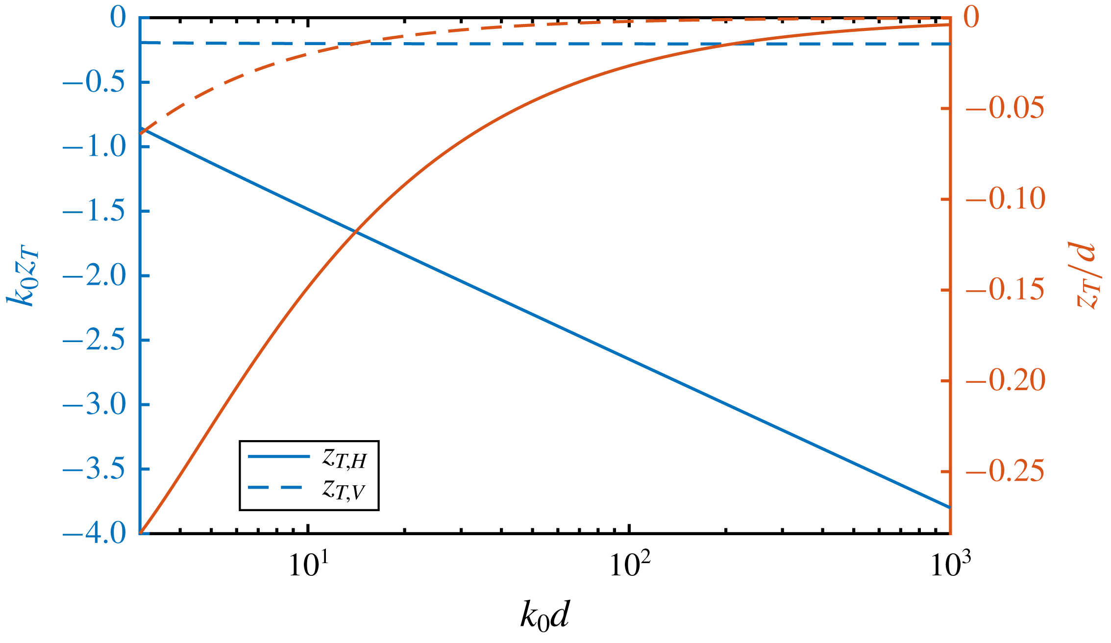
term to correct for the set-down. Figure 1 illustrates the dependence of these transition depths on
 $k_{0}d$
. The horizontal transition depth (continuous lines) can be a significant fraction of the water depth for moderate
 $k_{0}d$
(up to
 $z_{T,H}/d=-0.28$
for
 $k_{0}d=3$
), whereas the vertical transition depth (dashed lines) is generally given by
 $k_{0}z_{T,V}\approx -\text{log}(3/2)/2=-0.20$
, which becomes exact in the limit
 $k_{0}d\rightarrow \infty$
. In the shallow return flow limit (
 $d/\unicode[STIX]{x1D70E}\ll 1$
), the transition depths (2.9) also correspond to the depths below which the horizontal Lagrangian velocity becomes negative and the vertical Lagrangian velocity becomes negative (in front of the packet) or positive (behind the packet), respectively (cf. (2.3)).
Transition depths (2.9) defined as the depths where the horizontal (continuous lines) and vertical Lagrangian (dashed lines) displacements are zero owing to cancellation of their Stokes drift and Eulerian return flow components. The colours correspond to the left and right vertical axes, which are scaled differently.

3 Experimental methodology
3.1 Set-up, wave generation and data acquisition
We carried out experiments in the
 $35~\text{m}$
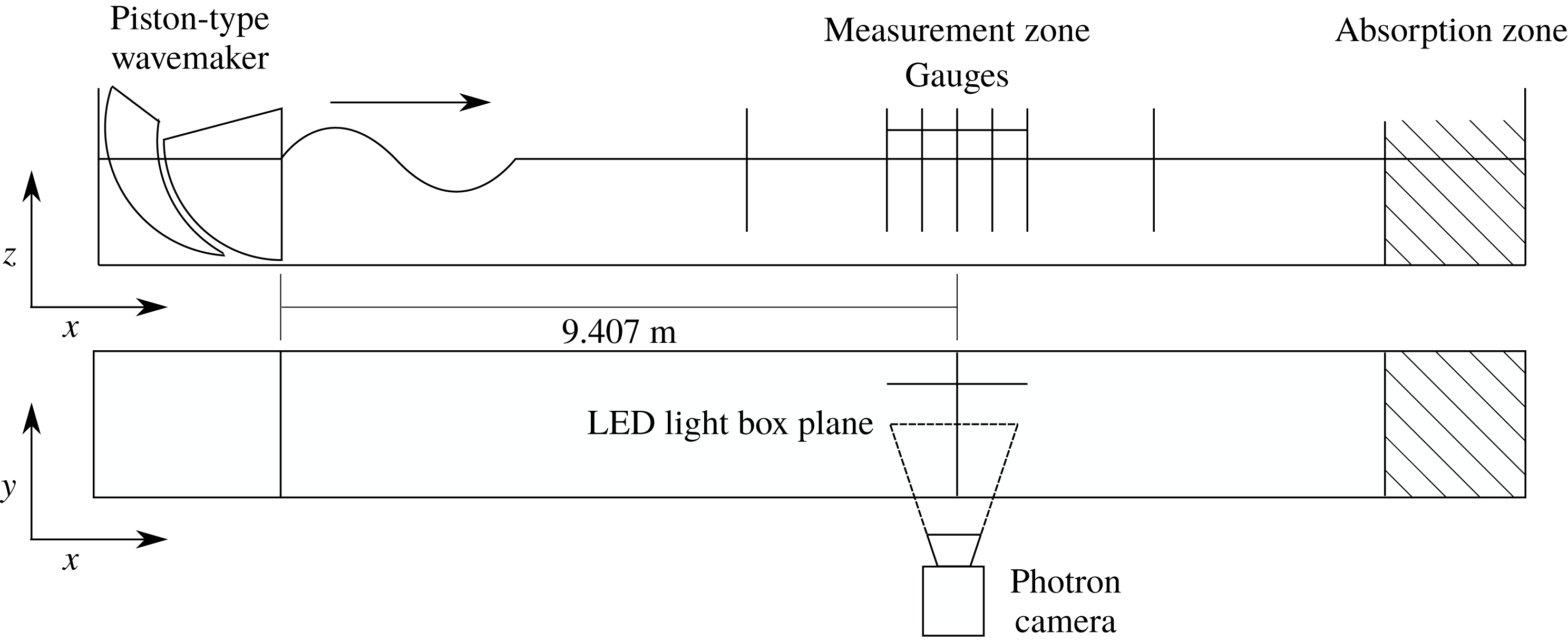
flume in the COAST (Coastal, Ocean and Sediment Transport) Laboratory at the University of Plymouth, UK. Our visualization experiments are illustrated in figure 2. The flume has a width of
 $0.6~\text{m}$
and was filled to a depth
 $d=0.5~\text{m}$
. We used a piston-type wavemaker to generate a focused wave group with a spectral shape that linearly focuses to a Gaussian packet
 $A_{0}=a_{0}\exp (-(x_{f}-c_{g,0}t)^{2}/2\unicode[STIX]{x1D70E}^{2})$
at a measurement zone located
 $x_{f}=9.407~\text{m}$
from the resting position of the wavemaker (measured free surface elevations are included in figure 9 in appendix A). Although the paddles were controlled with a combination of first- and second-order signals based on Schäffer (Reference Schäffer1996), subharmonic error waves are not expected to play a significant role for the deep-water waves examined here (Whittaker et al.
Reference Whittaker, Fitzgerald, Raby, Taylor, Orszaghova and Borthwick2017). A resistance-type wave gauge provided
 $128~\text{Hz}$
free surface elevation measurements at the focus location; the measured free surface signals provided the parameters used to predict the theoretical particle displacements for each experiment. A light-emitting diode (LED) light box located at the measurement zone (offset in the cross-flume direction from the wave gauge) illuminated the motions of small near-neutrally buoyant particles in a plane, which were captured by a camera located outside of the flume. Camera calibration details are given in § B.1.
The ‘Plascoat’ particles were approximately
 $150~\unicode[STIX]{x03BC}\text{m}$
in diameter, small enough to be considered dynamically unimportant. Although the particles were slightly positively buoyant, their upward settling velocities were small or at least slowly varying compared to their motion beneath the free surface waves (see § 3.3). The particles were effectively uniformly mixed throughout the measurement zone, which was achieved by adding new particles between experiments when necessary, mixing up the water column and waiting for the flume to become quiescent before starting experiments. Because of the light sheet, we only tracked a thin slice of particles in the (
 $x$
–
 $z$
)-plane. The camera field of view captured half the depth at a time. To obtain a complete distribution with depth, we thus repeated the same experiment twice.
After propagating through the measurement zone, the dispersed wave groups were absorbed by foam wedges within an ‘absorption zone’ located at the downstream end of the wave flume. The measurement zone was located far enough from the wavemaker to minimize the effects of evanescent modes from the wavemaker. To ensure near-quiescent initial conditions for each experiment the flume was allowed to settle for
 $10~\text{min}$
between experiments. Although negligible free surface motions remained after this time period, some slow circulations lingered within the subsurface velocity field; these ‘background particle velocities’ were removed during post-processing of the particle trajectories, as described below. The settling time of
 $10~\text{min}$
was short enough that the slightly positively buoyant particles remained evenly distributed throughout the water column at the start of each experiment.
Experimental set-up used to obtain particle tracking velocimetry (PTV) measurements of trajectories below focused wave groups generated by a piston-type wavemaker in the 35 m flume in the COAST Laboratory at the University of Plymouth.

3.2 Matrix of experiments
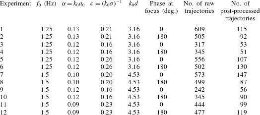
We conducted 12 experiments, as outlined in table 2, with experiment 1 conducted 10 times to determine repeatability. Frequencies
 $f_{0}$
were chosen such that the water depth is deep (
 $k_{0}d\gtrapprox 3$
); amplitudes
 $a_{0}$
such that second-order motions are large enough to measure, but not too large so that effects beyond second order play a role; and the bandwidth parameter
 $\unicode[STIX]{x1D716}=1/(k_{0}\unicode[STIX]{x1D70E})$
such that the wave group is still quasi-monochromatic (see van den Bremer & Taylor Reference van den Bremer and Taylor2016), but the wave groups not so long that reflections play a role. Having defined
 $\unicode[STIX]{x1D716}$
based on length scales in the physical domain and for a Gaussian group, we can obtain an estimate of the number of waves per group of
 $4\unicode[STIX]{x1D70E}/\unicode[STIX]{x1D706}_{0}=2/(\unicode[STIX]{x03C0}\unicode[STIX]{x1D716})\approx 2.5{-}4$
(cf. table 2 and figure 9 in appendix A). We investigated both crest-focused (CF) and trough-focused (TF) wave groups, for which frequencies have phases of
 $0$
or
 $\unicode[STIX]{x03C0}$
at focus, respectively.
Matrix of experiments.

3.3 Data processing and removal of background motion
The recorded images were processed using the Streams software package, a specialist package for flow visualization applications (Nokes Reference Nokes2014) (see § B.2). Lagrangian paths were calculated for particles that had been continuously matched for at least
 $\pm 6T_{g}$
with
 $T_{g}=\unicode[STIX]{x1D70E}/c_{g,0}$
either side of the time of focus. Despite the settling time between experiments, we found persistent background motion of the particles on a time scale much greater than the linear motion and the motion associated with Stokes drift and the Eulerian return flow beneath the group.
This background motion consists of a combination of upward settling of particles, long waves or ‘seiche modes’ that decay very slowly in the flume and Ekman-type circulation that result from small air flows over the surface that cannot be entirely eliminated in the laboratory. We can estimate the (upward) Stokes settling velocity for our spherical particles as
 $w=(2/9)((\unicode[STIX]{x1D70C}_{w}-\unicode[STIX]{x1D70C}_{p})/\unicode[STIX]{x1D70C}_{w})(gR^{2}/\unicode[STIX]{x1D708})=0.47~\text{mm}~\text{s}^{-1}$
, where we have used
 $\unicode[STIX]{x1D70C}_{p}=0.96~\text{g}~\text{cm}^{-3}$
(density of the particle),
 $\unicode[STIX]{x1D70C}_{w}=0.998~\text{g}~\text{cm}^{-3}$
(density of water),
 $\unicode[STIX]{x1D708}=1.0\times 10^{-6}~\text{m}^{2}~\text{s}^{-1}$
(kinematic viscosity) and
 $R=75\times 10^{-6}~\text{m}$
(radius of the particle). We can also estimate the velocity associated with a linear long wave of amplitude
 $a=0.1~\text{mm}$
(probably the smallest that can be detected by the gauges) to be
 $u=a\sqrt{g/d}=0.44~\text{mm}~\text{s}^{-1}$
. For comparison, the Stokes drift near the surface (
 $z=0$
) and at the point of focus is
 $u_{S}=c_{p,0}\unicode[STIX]{x1D6FC}^{2}=21~\text{mm}~\text{s}^{-1}$
for
 $c_{p,0}=1.25~\text{m}~\text{s}^{-1}$
(
 $f_{0}=1.25~\text{Hz}$
) and
 $\unicode[STIX]{x1D6FC}=0.13$
(see table 2). For the same case, the return flow velocity is
 $u_{E}=c_{p,0}\unicode[STIX]{x1D6FC}^{2}/(2k_{0}d-1/2)=3.6~\text{mm}~\text{s}^{-1}$
for
 $d=0.5~\text{m}$
. Fortunately, all these background motions vary more slowly than the waves and their induced mean flows and we can remove these by fitting to the background motion before and after the arrival of the group. The Lagrangian displacements were calculated after removal of this slow background motion, and the quality of the trajectories assessed, resulting in a smaller number of post-processed compared to raw trajectories, as reported in table 2.
When visually assessing the quality of the trajectories, we dismissed particles with incompletely recorded trajectories and particles for which our automatic criterion for identifying the focus time, namely the time at which the horizontal velocity reached a maximum, was not successful. The displacements were calculated between
 $t=-3T_{g}$
and
 $t=+3T_{g}$
, with
 $t=0$
corresponding to the focus point,
 $T_{g}=\unicode[STIX]{x1D70E}/c_{g,0}$
denoting the group period, and the limits chosen so that the overlying wave group has effectively zero amplitude. The trajectories recorded for times outside this window, during which there was no overlying wave group, were then used to fit to and then remove background motion. To do so, we considered four fitting methods and selected the one that minimized the displacement due to the background motion over the window
 $t=\pm 3T_{g}$
(see § B.3 for further details).
4 Results
4.1 Particle trajectories
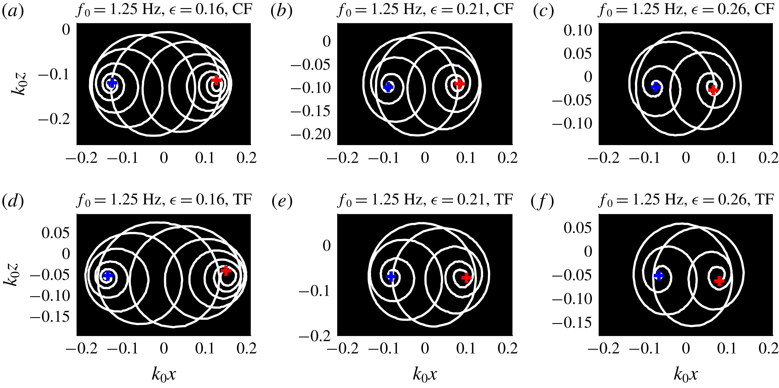
Experimental particle trajectories for particles near the surface below crest-focused (CF, top row) and trough-focused (TF, bottom row) wave groups for three different groups lengths
 $\unicode[STIX]{x1D70E}$
(columns), as denoted by
 $\unicode[STIX]{x1D716}=1/(k_{0}\unicode[STIX]{x1D70E})$
. The blue and red
 $+$
symbols denote experimentally determined initial and final particle positions, respectively.

Experimental particle trajectories for particles at different depths (rows) for three different groups lengths
 $\unicode[STIX]{x1D70E}$
(columns), as denoted by
 $\unicode[STIX]{x1D716}=1/(k_{0}\unicode[STIX]{x1D70E})$
. The blue and red
 $+$
symbols denote experimentally determined initial and final particle positions, respectively.

Figure 3 shows representative measured particle trajectories near the surface for crest-focused (CF, top row) and trough-focused (TF, bottom row) experiments with three different bandwidths (columns). Near the surface, the Stokes drift is dominant, the trajectories for shorter groups (larger
 $\unicode[STIX]{x1D716}$
) are made up from fewer orbits with smaller net horizontal displacements, and the vertically asymmetric relationship between crest-focused and trough-focused trajectories is clearest from comparing figures 3(c) and 3(f). The different columns in figure 4 show how particle trajectories vary with depth. Descending in the fluid, the net horizontal displacement transitions from positive near the surface (top row), via zero (middle row) to negative at depth (bottom row). At all depths, the linear wave signature remains present, although the magnitude of the orbits decreases. The horseshoe-shaped mean motion induced by the return flow is evident at depth (figure 4
g–i). In both figures 3 and 4, the blue and red symbols respectively denote the experimentally determined initial and final particle positions, which will be examined for all orbits below.
4.2 Net Lagrangian displacements
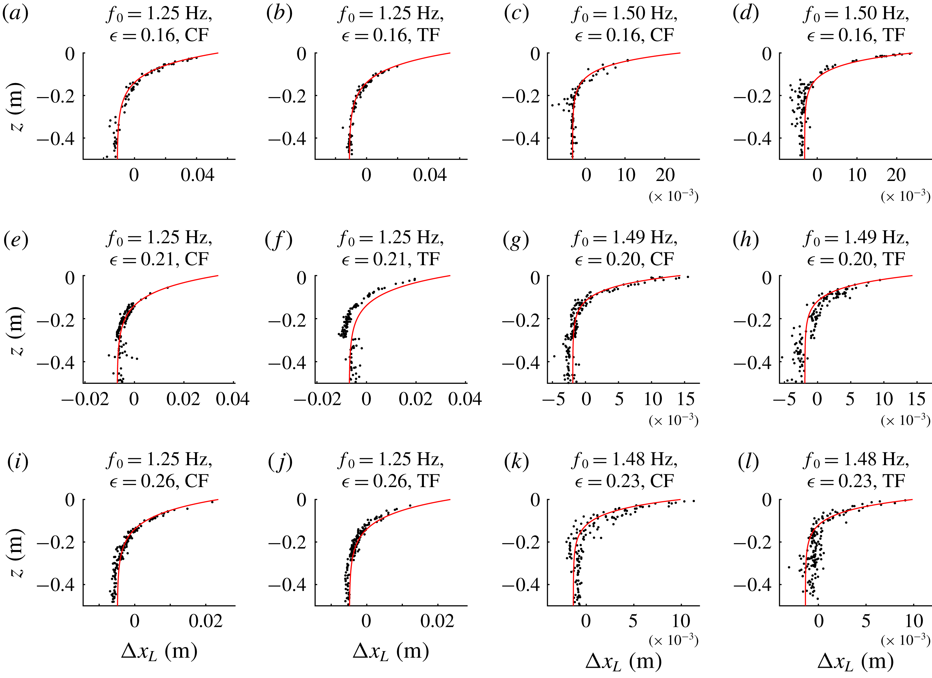
Net horizontal Lagrangian displacement from experiments (black dots) compared to theoretical predictions (red lines) for all experiments in table 2.

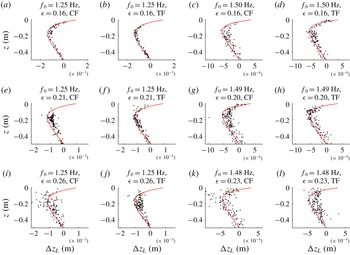
Maximum or minimum vertical Lagrangian displacement from experiments (black dots) compared to theoretical predictions (red lines) for all experiments in table 2.

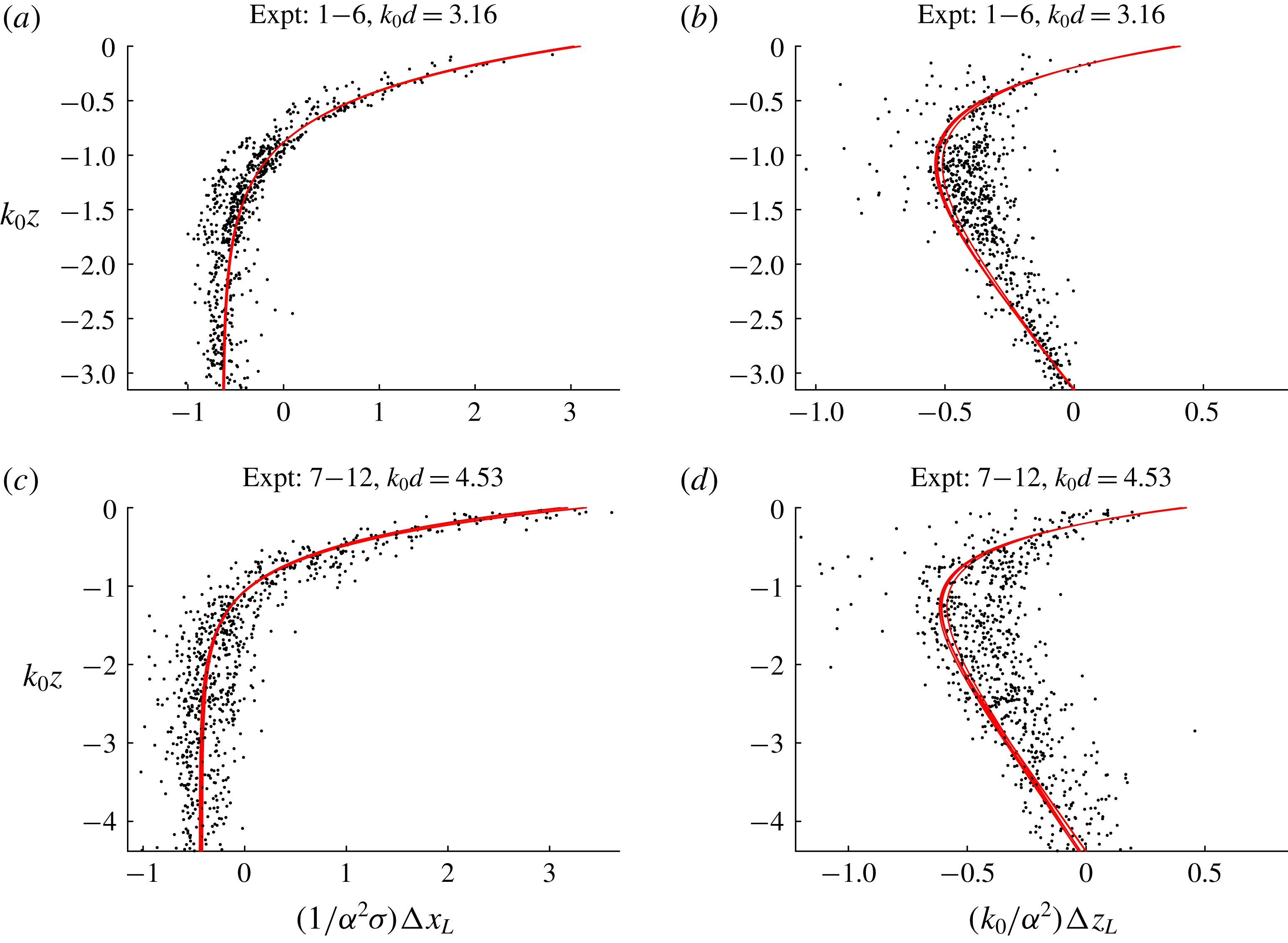
Scaled Lagrangian displacement from experiments (black dots) compared to theoretical predictions (red lines): (a,c) shows net horizontal displacement, (b,d) maximum or minimum vertical displacement; (a,b) correspond to
 $k_{0}d=3.16$
and (c,d) to 4.53, where
 $k_{0}d$
is the only non-dimensional parameter that cannot be scaled out. Note that several very slightly different theoretical curves are shown owing to small differences between the free surface elevation across experiments that cannot be scaled out.

After removal of background motion, figure 5 compares net horizontal Lagrangian displacement from experiments (black dots) to theoretical predictions (red lines) for all experiments. The theoretical predictions are evaluated from (2.5) and (2.7), where we evaluate
 $\unicode[STIX]{x1D714}_{0}$
from the peak of the surface elevation spectrum and compute
 $k_{0}$
from the linear dispersion relationship. Instead of fitting a Gaussian functional form, we numerically evaluate the time integrals in (2.5) and (2.7) over the envelopes extracted from the surface elevation measurements from the gauge, where we first remove bound waves from the spectrum, which has well-separated harmonics, using filtering. As expected based on irrotational theory for wave groups, the net positive displacements near the surface dominated by the Stokes drift are accompanied by opposing displacement at depth dominated by the return flow.
The changes in the net displacement due to changes in bandwidth (
 $\unicode[STIX]{x1D716}$
) that can be observed in figure 5 are indeed accurately predicted by our leading-order (in
 $\unicode[STIX]{x1D716}$
) results (2.5) and (2.7). Keeping
 $k_{0}$
constant, increasing
 $\unicode[STIX]{x1D716}$
amounts to a reduction in the group length
 $\unicode[STIX]{x1D70E}$
with a consequent reduction in the net displacement, as predicted by (2.5) and (2.7). Although our expressions are only strictly valid in the narrow-banded limit
 $\unicode[STIX]{x1D716}\equiv 1/(k_{0}\unicode[STIX]{x1D70E})\rightarrow 0$
, higher-order terms only potentially arise at two orders higher in
 $\unicode[STIX]{x1D716}$
. Based on the values of
 $\unicode[STIX]{x1D716}$
considered here and the calculations performed in van den Bremer & Taylor (Reference van den Bremer and Taylor2016), we estimate the error associated with our narrow-banded assumption to be a few percent in the worst case.
Using a similar procedure, figure 6 compares the maximum or minimum vertical Lagrangian displacements underneath the centre of the group to their theoretical predictions (2.6) and (2.8). The upward displacement by the Stokes drift near the surface predicted by irrotational theory for groups is accompanied by the classical Eulerian set-down at greater depth and decreasing to zero linearly with
 $z$
to zero at the bottom (cf. (2.8)).
In both figures 5 and 6, the orbits near the surface are not always perfectly captured, which is a result of their larger size and the (reflective) free surface moving through the camera window. Although the scatter in the data is not insignificant for some experiments (addressed in § 4.3), they line up well with theoretical predictions, including the magnitude of the displacement by the Stokes drift and the return flow. Finally, figure 7 presents scaled (non-dimensional) Lagrangian displacements from the experiments, noting from (2.5)–(2.8) that all parameters can be scaled out except for
 $k_{0}d$
.
4.3 Repeatability
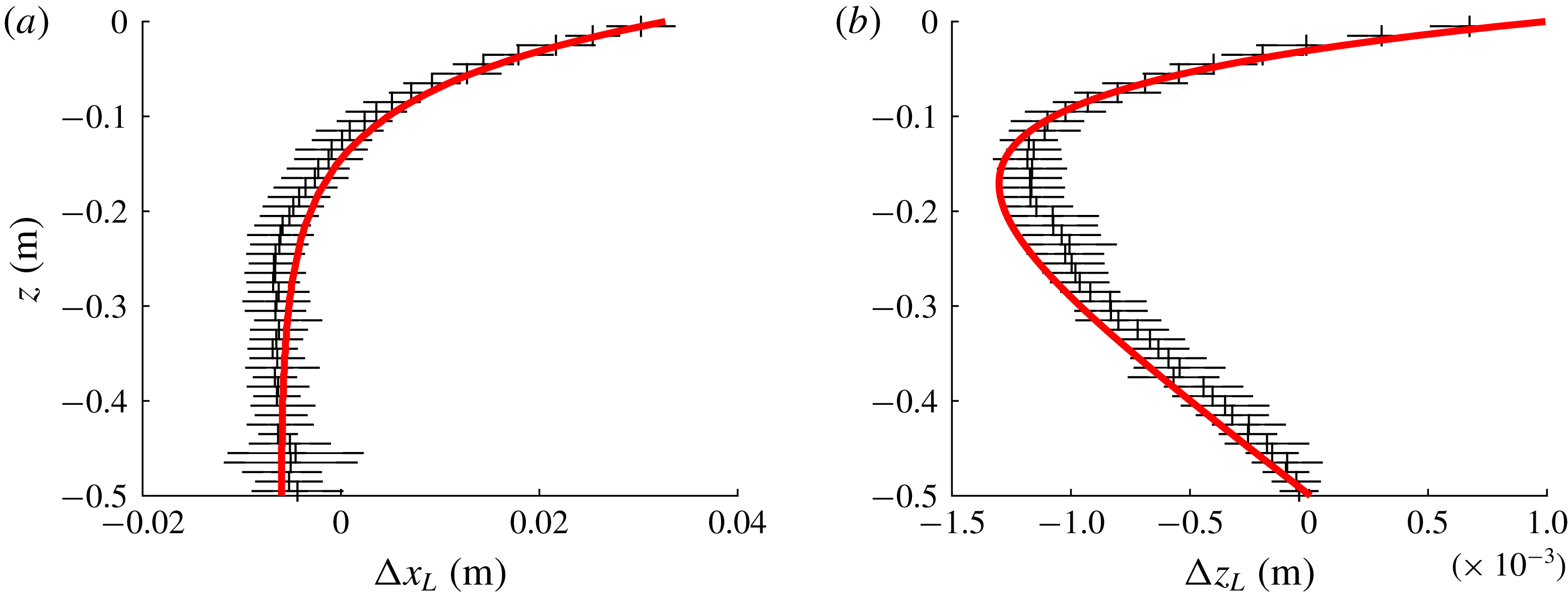
In order to assess repeatability of experiments and robustness of background motion removal, we conducted experiment 1 ten times. For both the horizontal and the vertical displacements, figure 8 demonstrates good agreement (to within two standard deviations) between experiments and theoretical predictions, notably including the positive vertical displacement by the Stokes drift in figure 8(b). Most of the variability for single experiments observed in figures 5–7 is likely to be due to unpredictable small residual motions present in the flume, which cannot be perfectly removed. In fact, the reason that the agreement with the theoretical solutions appears better for the horizontal displacements (cf. figure 5) than for the vertical displacements (cf. figure 6) is simply that the horizontal displacements are larger, making removal of background motion easier. Furthermore, the displacement associated with longer groups (smaller
 $\unicode[STIX]{x1D716}$
) is simply larger and thus easier to measure.
Confidence bands on the net horizontal (a) and the maximum or minimum vertical displacement (b) from 10 repeats of experiment 1 with the red lines denoting theoretical predictions. The error bars correspond to two standard deviations either side of the mean.

5 Conclusions
This paper has reported on an experimental study of Lagrangian trajectories underneath uni-directional deep-water surface gravity wave groups and has demonstrated visually their wave-induced Eulerian return flows as well as their Stokes drifts in experiments. Our quasi-monochromatic small-amplitude non-breaking experimental observations are in good agreement with leading-order solutions to the irrotational water wave equations. We have also shown that the Stokes drift for groups has both a horizontal and a vertical component, where the former results in a net displacement, whereas the latter leads to a temporary positive set-up for particles a small distance below the centre of a group, defined by a ‘transition’ depth. Such a non-zero vertical Stokes drift is contentious in equations of the Craik & Leibovich (Reference Craik and Leibovich1976)-type (McWilliams Reference McWilliams2016; Mellor Reference Mellor2016), but has been predicted to affect Lagrangian buoy records (Herbers & Janssen Reference Herbers and Janssen2016). For the relatively short, yet still quasi-monochromatic, groups we have examined, boundary layers do not have sufficient time to form and result in streaming of Lagrangian particles. Based on a typical velocity of
 $a_{0}\unicode[STIX]{x1D714}_{0}=0.16~\text{m}~\text{s}^{-1}$
for
 $a_{0}=0.021~\text{m}$
and
 $\unicode[STIX]{x1D714}_{0}=7.9~\text{rad}~\text{s}^{-1}$
and taking the amplitude
 $a_{0}$
as the typical length scale, we obtain a Reynolds number of
 $3.5\times 10^{3}$
(laminar). If we take the group length scale
 $\unicode[STIX]{x1D70E}=1.0~\text{m}$
as the characteristic length scale (for
 $f_{0}=1.25~\text{Hz}$
and
 $\unicode[STIX]{x1D716}=0.16$
), we can estimate the boundary layer thickness that can develop over this scale as
 $\unicode[STIX]{x1D6FF}=4.91\sqrt{(\unicode[STIX]{x1D70E}\unicode[STIX]{x1D708})/(a_{0}\unicode[STIX]{x1D714}_{0})}=0.012~\text{m}$
(Blasius solution for a laminar boundary layer over a plate). This is too small to play a role in our measurements. Furthermore, these short groups avoid the set-up of a closed-flume return flow associated with periodic waves, which may transport vorticity, be difficult to control experimentally and could account for some of the confusion in the literature. Although boundary layers, the convection and conduction of vorticity and breaking can probably explain the observed net drift and its depth variation in the majority of laboratory experiments, the finding by Smith (Reference Smith2006) of Eulerian counterflows occurring that completely cancel the Stokes drift variations at the surface for wave groups in field data is left unexplained.
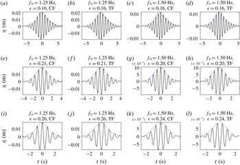
Measured free surface elevation signals for the 12 experiments in table 2: the dashed blue lines denote the envelopes obtained using a Hilbert transform.

Although experimental studies, including the present one, have focused exclusively on particles that behave as perfect Lagrangian tracers, modelling of transport of particles of all sizes and shapes in the upper ocean will require consideration of particle inertia (Eames Reference Eames2008; Santamaria et al. Reference Santamaria, Boffetta, Martins Afonso, Mazzino, Onorato and Pugliese2013) and anisotropy (DiBenedetto & Ouellette Reference DiBenedetto and Ouellette2018; DiBenedetto, Ouellette & Koseff Reference DiBenedetto, Ouellette and Koseff2018), as well as ‘surfing’ of particles near the surface (Deike et al. Reference Deike, Pizzo and Melville2017; Pizzo Reference Pizzo2017). Future work will examine these effects experimentally.
Acknowledgements
T.S.v.d.B. was supported by a Royal Academy of Engineering Research Fellowship. The authors would like to acknowledge J. Vanneste and C. Higgins for demonstrating that the net displacement (2.7) is not a function
 $z$
and W. Young for pointing out that there can be a vertical Stokes drift for irrotational water wave groups.
Appendix A. Measured free surface elevation signals
Figure 9 shows the unfiltered measured free surface elevation signals for the 12 experiments in table 2.
Appendix B. Experimental procedure and data processing
B.1 Camera settings and calibration
During the experiments, an LED light box located above the flume illuminated a two-dimensional plane approximately 1 m long and 10 mm thick. Ambient lighting was removed during these experiments, to maximize the contrast between the illuminated particles and the image background. A Photron SA4 high-speed camera captured the particle motions within the plane illuminated by the LED light box. Each experiment was repeated multiple times to ensure complete coverage of the depth and some overlap between different camera windows as a result. The camera captured images at
 $125~~\text{frames}~\text{s}^{-1}$
, with a resolution of
 $1024$
by
 $1024~\text{pixels}$
and a shutter speed of
 $1/125~\text{s}$
(i.e. opening the shutter for the duration of image acquisition). This shutter speed achieved an acceptable compromise between the requirements of obtaining very sharp images (requiring a high shutter speed) and allowing sufficient light to enter the CCD of the camera during each image (requiring a low shutter speed). Before conducting each experiment, the camera captured a calibration image of a ruler, allowing quantification of the pixel scale and any distortion in the images (barrel-pincushion distortions were found to be negligible for these tests). The image was calibrated by placing a ruler in the light sheet.
B.2 Image processing and particle tracking
The particles within each image were identified using a dual threshold algorithm, which first searched the image for pixels with an intensity greater than a particular threshold, identified the maximum pixel intensity within the group of pixels and finally defined the particle boundaries based on a fraction of this maximum intensity. This algorithm has the advantage of correctly identifying stationary and moving particles within a range of lighting conditions. The identified particles were subsequently matched between frames using an ‘auction’ optimization algorithm. This auction algorithm optimized the particle matches by minimizing the total cost of all potential matches for each successive pair of frames, where the cost was first assigned based on particle distance, then based on the (matched) particle velocities in a small region. The velocities of matched particles were finally used to generate additional matches where appropriate.
B.3 Removal of background motion
In order to remove background motion, we first centre the signal around the time of focus, chosen as the time of the maximum horizontal velocity, so that it corresponds to
 $t=0$
and then consider four ways of fitting to the background motion in the signals
 $(x(t),z(t))$
:
(i) linear fit to the
 $x$
-displacement prior to wave group arrival over
$(-6T_{g},-3T_{g})$
and quadratic fit to the
$z$
-displacement before and after wave group arrival over
$(-6T_{g},-3T_{g})$
and
$(3T_{g},6T_{g})$
;
(ii) linear fit to the
$x$
-displacement prior to wave group arrival over
$(-9T_{g},-3T_{g})$
and quadratic fit to the
$z$
-displacement before and after wave group arrival over
$(-9T_{g},-3T_{g})$
and
$(3T_{g},9T_{g})$
;(iii) linear fit to the
$x$
-displacement prior to wave group arrival over
$(-12T_{g},-3T_{g})$
and quadratic fit to the
$z$
-displacement before and after wave group arrival over
$(-12T_{g},-3T_{g})$
and
$(3T_{g},12T_{g})$
;(iv) linear fit to the
$x$
-displacement and quadratic fit to the
$z$
-displacement before and after wave group arrival over
$(-9T_{g},-3T_{g})$
and
$(3T_{g},9T_{g})$
;


where we estimated the group velocity
 $c_{g,0}$
and hence the group period
 $T_{g}$
from the spectral peak of the measured free surface time series.
All trajectories were visually inspected to ensure the orbit was complete and the focus location correctly identified. Of the four fitting methods, we selected the method that minimized the net ‘background’ displacement of the particle within the fit windows for each trajectory. After satisfactory processing of the particle orbits, the net displacements were calculated between
 $-3T_{g}$
and
 $3T_{g}$
.