1. Introduction
Discovering causality has long been the central focus of scientific research (Camps-Valls et al. Reference Camps-Valls, Gerhardus, Ninad, Varando, Martius, Balaguer-Ballester, Vinuesa, Diaz, Zanna and Runge2023; Martínez-Sánchez et al. Reference Martínez-Sánchez, Arranz and Lozano-Durán2024). Despite rich data from experiments and simulations, extracting cause-and-effect relationships from complex flow phenomena remains a challenging task (Lozano-Durán et al. Reference Lozano-Durán, Bae and Encinar2020; Lozano-Durán & Arranz Reference Lozano-Durán and Arranz2022). Randomised controlled trials, the gold standard for causal analysis, are often infeasible in such systems. This underscores the need for efficient causal inference of complex flows. To this end, data-driven causal analysis emerges as a promising solution, where causality is identified by detecting information transfer within a large amount of data. To illustrate this, consider variable
 $p$
as the cause of variable
 $q$
. It can be posited that specific information must initially appear in variable
 $p$
and subsequently be transmitted to variable
 $q$
. Various algorithms have been developed to quantify the transfer of information between variables. Typical methods include Granger causality in economics (Granger Reference Granger1969), which defines causality as the contribution of one variable to the prediction of another. Effective information (Tononi & Sporns Reference Tononi and Sporns2003), a concept from network science, quantifies causality as the difference between determinism and degeneracy within a dynamical system. Transfer entropy (Schreiber Reference Schreiber2000) is a nonlinear causal inference method that uses Shannon entropy to measure the uncertainty between variables. If the presence of variable
 $p$
diminishes the uncertainty of variable
 $q$
, a causal relationship is indicated from
 $p$
to
 $q$
.
Data-driven causal analysis has the potential to offer valuable solutions to a range of challenging problems in the field of fluid dynamics. Tissot et al. (Reference Tissot, Lozano-Durán, Cordier, Jiménez and Noack2014) utilised Granger causality to examine the causal relationships between the various velocity components in the logarithmic layer of wall turbulence. Their findings indicated that streak breakdowns initiate jets that are perpendicular to the wall surface. Lozano-Durán et al. (Reference Lozano-Durán, Bae and Encinar2020) applied transfer entropy to examine causalities between energy-containing eddies, revealing similar causal patterns between the buffer layer and the logarithmic layer. Lozano-Durán et al. (Reference Lozano-Durán, Constantinou, Nikolaidis and Karp2021) studied the impact of modifying linear terms by introducing controls into self-sustaining wall turbulence, revealing the mechanism of linear energy transfer from mean flow to fluctuating velocities. These studies provide useful information for understanding wall turbulence from the perspective of causality. In a study of isotropic turbulence, Jiménez (Reference Jiménez2018) successfully identified regions of importance by applying perturbations to a specific area and observing the resulting effects. This method was applied to two-dimensional isotropic turbulence (Jiménez Reference Jiménez2018) and three-dimensional isotropic turbulence (Encinar & Jiménez Reference Encinar and Jiménez2023). Causal analysis also facilitates the understanding of fluid–structure Interaction phenomena. Zhang et al. (Reference Zhang, Rosen, Peterson and Porfiri2018) revealed the causal relationship between tandem wings in uniform airflow using transfer entropy. Bagchi, Unni & Saha (Reference Bagchi, Unni and Saha2023) analysed the relationship between structural oscillation and Reynolds number in jet-induced vibrations of a cantilever beam using Pearson correlation and Granger causality. Wang et al. (Reference Wang, Chu, Lozano-Durán, Helmig and Weigand2021, Reference Wang, Lozano-Duran, Helmig and Chu2022) investigated boundary-layer–porous-media interactions using transfer entropy, revealing how permeability affects the intensity, time scale and spatial extent of these interactions. Furthermore, causal analysis has been used to investigate the association between pressure fluctuation at various locations within a jet (Omata & Tsutsumi Reference Omata and Tsutsumi2020) to identify the regions from which aerodynamic noise originates. Martínez-Sánchez et al. (Reference Martínez-Sánchez, Arranz and Lozano-Durán2024) decompose causalities into synergistic, unique and redundant components (SURD), revealing a top-down causal effect from outer-layer velocity to the inner layer in wall turbulence. Their follow-up study (Martínez-Sánchez & Lozano-Durán Reference Martínez-Sánchez and Lozano-Durán2025) further demonstrates that causality can be state-dependent, and proposes a state-aware SURD framework applicable to such scenarios. We also note that modern explainability tools (e.g. SHAP) have been applied to identify dynamically influential regions in complex turbulent flows (Cremades et al. Reference Cremades2024, Reference Cremades, Hoyas and Vinuesa2025). While not a formal inference in the Granger or Pearl sense, SHAP is implicitly grounded in a counterfactual reasoning framework, thereby offering a causally inspired perspective for interpreting black-box models.
Due to the high dimensionality of complex flows, direct causal analysis on flow data is nearly infeasible. As an alternative, causal analysis on reduced-order models (ROMs) is a more practical way, which has been supported by several works (Tissot et al. Reference Tissot, Lozano-Durán, Cordier, Jiménez and Noack2014; Martínez-Sánchez et al. Reference Martínez-Sánchez, López, Le Clainche, Lozano-Durán, Srivastava and Vinuesa2023). Such ROMs represent complex flow systems with low-dimensional manifolds, enabling efficient analysis, prediction and flow control (Galletti et al. Reference Galletti, Bruneau, Zannetti and Iollo2004; Akhtar Reference Akhtar2008; Rigas et al. Reference Rigas, Oxlade, Morgans and Morrison2014; Guastoni et al. Reference Guastoni, Güemes, Ianiro, Discetti, Schlatter, Azizpour and Vinuesa2021). Various ROMs have been developed, for example: (i) proper orthogonal decomposition (POD) (Lumley Reference Lumley1967; Sirovich Reference Sirovich1987; Towne, Schmidt & Colonius Reference Towne, Schmidt and Colonius2018; Mendez, Balabane & Buchlin Reference Mendez, Balabane and Buchlin2019), which decomposes flow snapshots into a series of orthogonal modes ordered by energy; (ii) dynamic mode decomposition (Rowley et al. Reference Rowley, Mezić, Bagheri, Schlatter and Henningson2009; Schmid Reference Schmid2010; Chen, Tu & Rowley Reference Chen, Tu and Rowley2012; Noack et al. Reference Noack, Stankiewicz, Morzyński and Schmid2016; Le Clainche & Vega Reference Le Clainche and Vega2017), rooted in Koopman theory, breaks down flow snapshots into a series of dynamic modes characterised by single frequencies and exponential growth rates; (iii) the Galerkin model (Deane et al. Reference Deane, Kevrekidis, Karniadakis and Orszag1991; Holmes Reference Holmes2012), which provides a unique analytical perspective for dimension reduction, and after Galerkin projection, the governing equations are transformed into a set of ordinary differential equations (ODEs); and (iv) machine-learning-based ROMs (Kaiser et al. Reference Kaiser, Noack, Cordier, Spohn, Segond, Abel, Daviller, Östh, Krajnović and Niven2014; Brunton, Noack & Koumoutsakos Reference Brunton, Noack and Koumoutsakos2020; Murata, Fukami & Fukagata Reference Murata, Fukami and Fukagata2020; Solera-Rico et al. Reference Solera-Rico, Sanmiguel Vila, Gómez-López, Wang, Almashjary, Dawson and Vinuesa2024), which have emerged in recent years and are drawing growing interest from researchers.
Generally speaking, data-driven causal analysis has provided a valuable perspective, expanding our focus from individual modes to modal interactions. However, the aforementioned data-driven causal analyses have limitations. As purely data-driven approaches, they may yield computationally plausible but factually false results (Smirnov Reference Smirnov2013; Stokes & Purdon Reference Stokes and Purdon2017). Without sufficient prior knowledge for guidance, it is difficult to validate or interpret the obtained results. This issue is of particular concern in the field of physical research, as physical conclusions must be drawn with rigour.
In this work, we present a hybrid causal analysis framework for low-dimensional Galerkin models, through combining both equation-based analysis and the proposed Galerkin-based Granger causality (GGC). These two methods identify causality from qualitative and quantitative perspectives, respectively, and can be validated against each other. In particular, it compensates for the inherent uncertainty of data-driven methods by integrating domain knowledge. The effectiveness of this method is validated in a low-dimensional Galerkin model of turbulent shear flows, especially of the effect of nonlinear terms on the dynamics. Two types of quadratic interactions are identified, and the propagation of nonlinear terms is represented by a directed cause-and-effect network. Using the causal relationship, a causality-guided flow control is performed to demonstrate how causalities can be used in practice, where extreme events in turbulence have been successfully suppressed. To further validate the applicability of the proposed method in complex, real-world scenarios, we further analyse the causal relationship in a turbulent lid-driven cavity-flow problem.
This paper is organised as follows. Sections 2 and 3 elaborate on the theoretical foundations of the Galerkin model and classical Granger causality, respectively. In § 4, a GGC is proposed. In § 5, we apply equation-based and GGC analyses to the turbulent shear flow model proposed by Moehlis, Faisst & Eckhardt (Reference Moehlis, Faisst and Eckhardt2004). Qualitative and quantitative causal findings are provided, and a causality-guided flow control is illustrated. Finally, conclusions and perspectives are presented in § 6. The mode definition in the shear flow model and additional application of GGC on turbulent cavity flow are presented in Appendices A and B, respectively. The source codes from this research are publicly available.
2. Galerkin model
The Galerkin model is one of the commonly used approaches to construct ROMs, using first principles of the Navier–Stokes equations. It projects governing equations onto spatially orthogonal modes to obtain a low-dimensional representation of flows, leading to a set of ODEs that describe the temporal evolution of mode coefficients. For example, considering the incompressible Navier–Stokes equations
 \begin{align} \begin{aligned} \boldsymbol{\nabla }\boldsymbol{\cdot }\boldsymbol{u} &= 0, \\ \frac {\partial \boldsymbol{u}}{\partial t} + (\boldsymbol{u} \boldsymbol{\cdot }\boldsymbol{\nabla }) \boldsymbol{u} &= -\boldsymbol{\nabla }p + \frac {1}{Re}\Delta \boldsymbol{u} + \boldsymbol{f}. \end{aligned} \end{align}
where
 $p$
represents pressure, and
 $\boldsymbol{f}$
represents body force. The velocity
 $\boldsymbol{u}$
is divided into two components: a constant mean flow velocity
 ${\boldsymbol {u}}_{0}$
and a fluctuating velocity
 $\boldsymbol{u}^{\prime }$
that varies over time. After modal projection, the fluctuating velocity is decomposed into a linear combination of several modes. These velocity modes are mutually orthonormal, implying that the inner product of any two mode pairs is zero, i.e.
 $(\phi _i, \phi _j)_\varOmega = 0, (i \neq j)$
:
 \begin{align} \boldsymbol{u}(t) = \boldsymbol{u}_{0} + \boldsymbol{u}^{\prime }(t) = \boldsymbol{u}_{0} + \sum _{i=1}^{n} a_{i}(t) \boldsymbol{\phi }_{i}, \end{align}
where
 $n$
is the number of modes. The decomposed velocity is then substituted into the incompressible Navier–Stokes equations. This results in the final Galerkin model, which is a set of nonlinear ODEs of mode coefficients:
 \begin{align} \frac {{\rm d}}{{\rm d}t}a_i = C_i + \frac {1}{Re}\sum _{j=1}^n L_{\textit{ij}} a_j + \sum _{j=1}^n \sum _{k=1}^n Q_{\textit{ijk}} a_j a_k. \end{align}
The constant term in the equation arises from the pressure gradient, external body force and mean flow velocity. In incompressible flows, the inner product of the pressure gradient and the velocity mode (the first term in (2.4)) is entirely dependent on the boundary conditions (Noack, Papas & Monkewitz Reference Noack, Papas and Monkewitz2005):
 \begin{align} C_i = -(\boldsymbol{\phi }_{i}, \boldsymbol{\nabla }p)_\varOmega + (\boldsymbol{\phi }_{i}, \boldsymbol{f})_\varOmega - (\boldsymbol{\phi }_{i}, (\boldsymbol{u}_0 \boldsymbol{\cdot }\boldsymbol{\nabla }) \boldsymbol{u}_0)_\varOmega + \frac {1}{Re} (\boldsymbol{\phi }_{i}, \Delta \boldsymbol{u}_0)_\varOmega . \end{align}
The linear term arises from viscous dissipation and the interaction between the mean flow velocity and the fluctuating velocity under convection:
 \begin{align} L_{\textit{ij}} = (\boldsymbol{\phi }_{i}, \Delta \boldsymbol{\phi }_{\kern-1pt j})_\varOmega - Re ( (\boldsymbol{\phi }_{i}, (\boldsymbol{u}_0 \boldsymbol{\cdot }\boldsymbol{\nabla })\boldsymbol{\phi }_{\kern-1pt j})_\varOmega + (\boldsymbol{\phi }_{i}, (\boldsymbol{\phi }_{\kern-1pt j} \boldsymbol{\cdot }\boldsymbol{\nabla })\boldsymbol{u}_0)_\varOmega ). \end{align}
All quadratic terms originate from nonlinear convection effects:
 \begin{align} Q_{\textit{ijk}} = -(\boldsymbol{\phi }_{i}, (\boldsymbol{\phi }_{\kern-1pt j} \boldsymbol{\cdot }\boldsymbol{\nabla })\boldsymbol{\phi }_k)_\varOmega . \end{align}
It is important to note that the selection of velocity modes is not without alternatives; however, it is preferable that these modes are capable of representing the primary features of the flow. Among the common approaches, projection on POD modes (Rempfer Reference Rempfer2000; Balajewicz, Dowell & Noack Reference Balajewicz, Dowell and Noack2013) and Fourier velocity modes (Waleffe Reference Waleffe1997; Moehlis et al. Reference Moehlis, Faisst and Eckhardt2004) are frequently used. In addition to projection-based techniques, an alternative pathway exists through system identification (Brunton, Proctor & Kutz Reference Brunton, Proctor and Kutz2016; Loiseau & Brunton Reference Loiseau and Brunton2018), where Galerkin equations are inferred directly from data-driven ROMs. Galerkin models offer the advantage of preserving the dominant features of unsteady flows with minimal computational cost, making them a preferable tool for studying complex flows (Rowley & Dawson Reference Rowley and Dawson2017). However, there are several drawbacks of the Galerkin models. For instance, their utilisation in compressible flows is considerably more complicated (Rowley, Colonius & Murray Reference Rowley, Colonius and Murray2004). Galerkin models are not well suited for accommodating arbitrary domain deformations or imposing complex boundary conditions (Loiseau, Noack & Brunton Reference Loiseau, Noack and Brunton2018), and may face challenges related to stability and conservation (Iollo, Lanteri & Désidéri Reference Iollo, Lanteri and Désidéri2000; Balajewicz et al. Reference Balajewicz, Dowell and Noack2013; Östh et al. Reference Östh, Noack, Krajnović, Barros and Borée2014). Despite the aforementioned limitations, Galerkin models offer distinct analytical advantages that facilitate causal analysis and its validation.
3. Granger causality
In 1969, the economist Clive Granger, motivated by Wiener’s theory of prediction (Wiener Reference Wiener1949), put forward the concept of Granger causality (Granger Reference Granger1969). Since its introduction, the method has been widely applied in numerous fields that involve data analysis (Freeman Reference Freeman1983; Hiemstra & Jones Reference Hiemstra and Jones1994; Ding, Chen & Bressler Reference Ding, Chen and Bressler2006; Smirnov & Mokhov Reference Smirnov and Mokhov2009). The principle of Granger causality is straightforward: if the prediction of variable
 $q$
significantly deteriorates when variable
 $p$
is excluded from a vector autoregressive model, then
 $p$
is said to be the Granger-cause of
 $q$
. A schematic illustration of classical Granger causality is shown in figure 1.
Schematic illustration of classical Granger causality. The computation of Granger causality from
 $x_1$
to
 $x_2$
(
 $\mathcal{F}_{1\to 2}$
) is depicted. This measure quantifies the increase in uncertainty of
 $x_2$
when past information from
 $x_1$
is omitted, evaluated by comparing the prediction errors of the full model and the reduced model (excluding
 $x_1$
history).

Specifically, to determine the Granger causality from
 $x_{p}$
to
 $x_{q}$
(denoted as
 $\mathcal{F}_{p\to q}$
), two auto-regressive with eXogenous inputs model with a time lag of
 $r$
are constructed: a full model including
 $\boldsymbol{x}_{p}$
and a reduced model excluding it. The prediction accuracy of these two models is then compared. The full model is
 \begin{align} \boldsymbol{x}_q^{t} = \sum _{i=1}^n\sum _{k=1}^{r} L_i^{(k)} \boldsymbol{x}_i^{t-k} + \boldsymbol{\varepsilon }_q, \end{align}
where
 $n$
denotes the total number of variables,
 $r$
denotes order of time lag,
 $\boldsymbol{x}_{q}^t$
represents the time sequence of the variable
 $ q$
in vector, from time index
 $r+1$
to
 $t$
,
 $\boldsymbol{x}_i^{t-k}$
represents the time sequence of the variable
 $ i$
in vector, delayed by an order of
 $k$
,
 $ L_i \boldsymbol{x}_i$
represents the linear regression term and
 $\boldsymbol{\varepsilon }_q$
is the model error vector. The reduced model is
 \begin{align} \boldsymbol{x}_q^{t} = \sum _{i=1}^n\sum _{k=1}^{r} \tilde {L}_i^{(k)} \boldsymbol{x}_i^{t-k} + \boldsymbol{\tilde {\varepsilon }}_{p\to q} \quad (i \neq p). \end{align}
Here, condition
 $i \neq p$
ensures that variable
 $\boldsymbol{x}_{p}$
is excluded from the reduced model. The tilde denotes quantities associated with the reduced model. If the exclusion of
 $\boldsymbol{x}_{p}$
impairs the prediction of
 $\boldsymbol{x}_{q}$
, the variance of
 $\tilde {\boldsymbol{\varepsilon }}_{p\to q}$
will exceed that of
 $\boldsymbol{\varepsilon }_{q}$
from the full model. The Granger causality from
 $\boldsymbol{x}_{p}$
to
 $\boldsymbol{x}_{q}$
is then defined as the log-ratio of these two error variances:
 \begin{align} \mathcal{F}_{p\to q} = \ln \frac {\text{var}(\tilde {\boldsymbol{\varepsilon }}_{p\to q})}{\text{var}(\boldsymbol{\varepsilon }_{q})}, \end{align}
where
 $\text{var}(\boldsymbol{\varepsilon })$
denotes the variance of the error vector. From the perspective of information theory, Granger causality quantifies the contribution of a variable to the dynamic prediction of others; its magnitudes may have a natural interpretation in terms of information-theoretic bits per unit time (Barnett & Seth Reference Barnett and Seth2014). Notably, self-causalities
 $\mathcal{F}_{i\to i}$
are excluded from computation (appearing as zero in the maps), as Granger causality focuses on inter-variable causalities. In addition, the self-history of each mode is expected to contribute strongly to predicting its own future. Granger causality also shares conceptual similarities with sensitivity analysis (Borgonovo & Plischke Reference Borgonovo and Plischke2016). Sensitivity analysis quantifies the sensitivity of outputs to variations in input parameters, i.e. typically by perturbing inputs within a defined range to assess model robustness. Granger causality specifically examines whether one time series can help predict another, thereby inferring potential causal relationships. In this sense, Granger causality can be seen as a specialised form of sensitivity analysis.
Despite its simplicity and intuitiveness, Granger causality imposes stringent definitions on its applicability. Numerous explicit or implicit assumptions serve as prerequisites for employing Granger causality (Shojaie & Fox Reference Shojaie and Fox2022):
-
(i) Temporal order: causality is temporally ordered, with causes preceding effects; instantaneous causality without time delay is not considered.
-
(ii) Stationarity: the statistical properties of data, such as variance and mean, are time-invariant.
-
(iii) Linearity: the interactions between variables are assumed to be linear and can be accurately described by an autoregressive model.
-
(iv) Known time lag: the extent to which causality exists in the history of variables is known and is represented by a fixed time lag.
-
(v) Complete system: it is assumed that the analysis incorporates all relevant variables and that there are no unmeasured confounders.
These prerequisites have been designed to ensure the accuracy and reliability of Granger causality, thereby avoiding spurious causality. However, in practice, they are difficult to fully satisfy. For example, many real-world multivariate time series are non-stationary (Safikhani & Shojaie Reference Safikhani and Shojaie2022); nonlinearity is a common feature in complex dynamical systems; it is also difficult to exclude all confounding factors without sufficient prior knowledge. These issues limit the application of Granger causality (Stokes & Purdon Reference Stokes and Purdon2017), especially in fluid dynamic problems. Therefore, we introduce a GGC, a modified framework specifically developed for causal inference in Galerkin-based flow systems.
4. Galerkin-based Granger causality
The proposed GGC retains the concept and framework of classical Granger causality, while it is tailored for systems following Galerkin-structured dynamics (e.g. Navier–Stokes equations projected onto low-dimensional bases). Given that Galerkin models inherently comprise constant, linear and quadratic terms, the GGC resembles a quadratic Granger causality in form.
-
(i) Nonlinearity: classical Granger causality does not account for complex nonlinear interactions. Inspired by the known structure of Galerkin equations (see (2.3)), the GGC retains essential linear terms while incorporating quadratic and constant terms. This allows GGC to model nonlinear dynamics more accurately.
-
(ii) Relaxed stationarity assumption: complex flows are highly time-variant, where different causal relationships may emerge at different stages as the flow develops. Stationarity is relaxed in the GGC. Instead, the time-variant property is captured by a windowed analysis strategy, as detailed below.
-
(iii) Fixed time delay: since the Galerkin model is described by first-order ODEs, the time lag/discrete time delay in GGC is set to 1. This helps to avoid overfitting (Johansen Reference Johansen1988), and also eliminates possible indirect causal links.
-
(iv) Windowed analysis: since causalities in complex unsteady flows may vary with time, the GGC first divides the time sequence into several windows of equal length (figure 2). Within each window, the causality is computed in parallel to discover short-term causality. The ensemble average of these short-term causalities is taken to reflect the long-term causality.
Schematic of the windowed analysis strategy of GGC. The time series of variables are equidistantly partitioned into intervals, with Granger causality applied to each interval to capture short-term causality, which are then ensemble-averaged to derive the averaged causality.

The window segmentation is governed by two parameters: the window length, which denotes the length of each segment, and the window overlap, which defines the shared length between consecutive windows. In this study, the overlap is simply selected as half of the window length, whereas the window length requires careful determination as it greatly affects the final results. We observed a trade-off in window length selection: it must be sufficiently long for reliable Galerkin model estimation yet short enough to capture short-term causality. To balance these requirements, we employ the causal discriminability index (CDI) as a selection criterion, which is formally defined later in (4.5).
Schematic illustration of modified Granger causality. The framework retains the core structure of classical Granger causality, with the addition of nonlinear and constant terms to align with the structure of Galerkin equations.

After the aforementioned modifications, the GGC is defined as follows. We start from a Galerkin model composed of
 $ n$
modes
 $(x_1, x_2, x_3, {\ldots} x_n)$
. First, a suitable window length is selected to segment the time series of the mode coefficient into
 $N$
equally spaced windows. To evaluate the causal effect
 $\mathcal{F}_{p\to q}$
, a full Galerkin model is constructed that uses all modes to predict mode
 $q$
in each window:
 \begin{align} \boldsymbol{x}_q^{t} = \sum _{i=1}^n L_i \boldsymbol{x}_i^{t-1} + \sum _{i,j=1,i\leqslant j}^n Q_{\textit{ij}} \boldsymbol{x}_i^{t-1} \boldsymbol{x}_{\kern-1pt j}^{t-1} + C + \boldsymbol{\varepsilon }_q, \end{align}
where
 $ \boldsymbol{x}_q^{t}$
is the coefficient of mode
 $ q$
in vector,
 $ L_i \boldsymbol{x}_i^{t-1}$
represents the linear terms,
 $ Q_{\textit{ij}} \boldsymbol{x}_i^{t-1} \boldsymbol{x}_{\kern-1pt j}^{t-1}$
denotes the quadratic terms, both delayed by an order of 1 (one time step),
 $ C$
is the constant term and
 $ \boldsymbol{\varepsilon }_q$
is the vector of prediction error. Subsequently, by removing all linear and quadratic terms involving mode
 $ p$
, the reduced Galerkin model is constructed:
 \begin{align} \boldsymbol{x}_q^{t} = \sum _{i=1}^n \tilde {L}_i \boldsymbol{x}_i^{t-1} + \sum _{i,j=1,i\leqslant j}^n \tilde {Q}_{\textit{ij}} \boldsymbol{x}_i^{t-1} \boldsymbol{x}_{\kern-1pt j}^{t-1} + \tilde {C} + \tilde {\boldsymbol{\varepsilon }}_{p\to q} \quad (i,j \neq p), \end{align}
where the constraint
 $ i,j \neq p$
excludes all terms involving mode
 $ p$
and
 $ \tilde {\boldsymbol{\varepsilon }}_{p\to q}$
is the corresponding error vector. In accordance with the classical Granger causality,
 $\mathcal{F}_{p\to q}$
in each analysis window is defined as the log-ratio of two variances:
 \begin{align} \mathcal{F}_{p\to q}^{i} = \ln \frac {\text{var}(\tilde {\boldsymbol{\varepsilon }}_{p\to q})}{\text{var}(\boldsymbol{\varepsilon }_q)}, \quad i = 1, 2, 3, \dots , N, \end{align}
where self-causalities
 $\mathcal{F}_{i\to i}$
are not computed and manually set to 0. By repeating the process in all windows, the short-term GGC for each window is obtained. Notably, this formulation allows for parallel computing, offering an advantage in computational speed. Taking the average of the results from all analysis windows, we obtain the long-term GGC of the entire sequence:
 \begin{align} \mathcal{F}_{p\to q} = \text{avg}(\mathcal{F}_{p\to q}^{1} + \mathcal{F}_{p\to q}^{2} + \cdots + \mathcal{F}_{p\to q}^{N}). \end{align}
The CDI is then defined as
 \begin{align} \text{CDI} = \frac {\text{std}(\mathcal{F}_{p \rightarrow q})}{\text{avg}(\mathcal{F}_{p \rightarrow q})} = \sqrt {\frac {1}{m-1}\sum _{p,q=1}^n \left (\mathcal{F}_{p \rightarrow q} - {\mathcal{\overline {F}}}\right )^2} / \mathcal{\overline {F}}, \quad p \neq q, \end{align}
where
 $m = n(n-1)$
represents the number of pairwise GGC,
 $\text{avg}(\mathcal{F}_{i \to j}) = \mathcal{\overline {F}} = ({1}/{m})\sum _{i,j=1}^n (\mathcal{F}_{i \rightarrow j} ),\ i \neq j$
represents the overall mean GGC value and
 $\text{std}(\mathcal{F}_{i \to j})$
denotes the overall standard deviation. Therefore, the CDI is defined as the ratio of the standard deviation to the mean GGC value, quantifying the discriminability of pairwise causality. An optimal window length enhances the distinction between strong and weak causal links, resulting in a higher CDI (see figure 10). Thus, we determine the window length by maximising the CDI.
Statistical tests are essential for distinguishing true causal relationships from spurious ones in causal inference. Standard tests for Granger causality, the F-test and likelihood ratio test (Shojaie & Fox Reference Shojaie and Fox2022), can be extended to our proposed GGC framework. However, when applied to nonlinear flow data, both tend to overestimate the significance and produce false positives, as detailed in the supplementary material availabe at https://doi.org/10.1017/jfm.2026.11553. As an alternative, we employ a permutation test based on time-shifted surrogates (Quian Quiroga et al. Reference Quian Quiroga, Kraskov, Kreuz and Grassberger2002; Andrzejak et al. Reference Andrzejak, Kraskov, Stögbauer, Mormann and Kreuz2003), which effectively removes secondary and spurious causalities. Its core idea is simple: for each candidate cause variable, we generate multiple surrogate time series by applying random cyclic time shifts (i.e. rotating the time series by a random lag; see figure 11
c). This procedure breaks any potential causality from the cause variable while preserving the intrinsic statistical properties of each series. We then compute GGC for plenty of these shifted surrogate pairs (typically 50–200 permutations) to construct an empirical null distribution under the hypothesis of no Granger causality. The
 $(1-\alpha )$
th quantile (e.g. the 95th percentile for
 $\alpha$
= 0.05) of this distribution is taken as the significance threshold. If the GGC value from the original data exceeds this threshold, we reject the null hypothesis and conclude that statistically significant Granger causality exists at level
 $\alpha$
. This allows us to reliably identify causal links from the quantitative GGC results.
We also emphasise some limitations of the proposed GGC method. (i) The quadratic formulation is specifically designed for Galerkin models of fluid flows and may not generalise to systems with different dynamical structures. (ii) Results can be influenced by hyperparameters such as window length and significance level in permutation tests, making careful selection and sensitivity analysis necessary before analysing the causal relations. (iii) In systems dominated by quadratic terms, GGC quantifies blended multivariate causal effect rather than isolated pairwise causality. For example, the quadratic term
 $a_j a_k$
of
 $\dot {a}_i$
inherently contains coupled influence from both
 $a_j$
and
 $a_k$
to
 $a_i$
, which cannot be distinguished independently. However, this is due to the strong coupling between triadic mode pairs (Kraichnan & Chen Reference Kraichnan and Chen1989) in Galerkin models. Enforcing strict pairwise causality (e.g. by omitting interaction terms) would thus fail to capture the true dynamics.
5. Application
In this section, the proposed GGC is validated through the application to an empirical Galerkin model for turbulent shear flows proposed by Moehlis et al. (Reference Moehlis, Faisst and Eckhardt2004). We begin by analysing the governing equations (i.e. the first principles) to represent the reference causality (§ 5.2). Next, we apply GGC to the same model based on simulation data, and show that the inferred causality closely matches the reference (§ 5.3). Through these analyses, we validate GGC and the robustness of the combined analysis. Useful insights into the causal interactions among Galerkin modes are also obtained. Then, causality-guided flow control is investigated to show how the analysis helps to distill control opportunities (§ 5.4). Finally, a comparison between the GGC and existing causal analysis methods is provided (§ 5.5).
Velocity contours of the nine modes in the turbulent shear flow model. Arrows denote velocity vectors, while the colour map (blue: low; red: high) indicates velocity magnitude.

5.1. Nine-equation turbulent shear flow model
Waleffe (Reference Waleffe1997) developed an eight-Fourier-mode ROM for turbulent shear flows based on Galerkin projection. This empirical model was later refined by Moehlis et al. (Reference Moehlis, Faisst and Eckhardt2004), where the ninth mode is introduced for correction. This model depicts three-dimensional turbulent shear flow induced by sinusoidal body forcing. The velocity is composed of nine Fourier velocity modes: the base profile (mode 1), streak (mode 2), downstream vortex (mode 3), spanwise flow (modes 4 and 5), normal vortex (modes 6 and 7), fully three-dimensional structure (mode 8) and modification of the base profile (mode 9), as shown in figure 4. Their detailed descriptions are presented in Appendix B. The spatial domain is specified as
 $0 \leqslant x \leqslant L_x, -1 \leqslant y \leqslant 1, 0 \leqslant z \leqslant L_z$
. By projecting the incompressible Navier–Stokes equations onto the nine velocity modes, the following system of ODEs is derived:
 \begin{align} \frac {{\rm d}a_1}{{\rm d}t} = \frac {\beta ^2}{Re} - \frac {\beta ^2}{Re} a_1 - \sqrt {\frac {3}{2}} \frac {\beta \gamma }{\kappa _{\alpha \beta \gamma }} a_6 a_8 + \sqrt {\frac {3}{2}} \frac {\beta \gamma }{\kappa _{\beta \gamma }} a_2 a_3, \\[-28pt] \nonumber \end{align}
 \begin{align} \begin{aligned} \frac {{\rm d}a_2}{{\rm d}t} = -\left ( \frac {4 \beta ^2}{3} + \gamma ^2 \right ) \frac {a_2}{Re} + \frac {5 \sqrt {2}}{3 \sqrt {3}} \frac {\gamma ^2}{\kappa _{\alpha \gamma }} a_4 a_6 - \frac {\gamma ^2}{\sqrt {6} \kappa _{\alpha \gamma }} a_5 a_7 \\ - \frac {\alpha \beta \gamma }{\sqrt {6} \kappa _{\alpha \gamma } \kappa _{\alpha \beta \gamma }} a_5 a_8 - \sqrt {\frac {3}{2}} \frac {\beta \gamma }{\kappa _{\beta \gamma }} a_1 a_3 - \sqrt {\frac {3}{2}} \frac {\beta \gamma }{\kappa _{\beta \gamma }} a_3 a_9, \end{aligned} \\[-28pt] \nonumber \end{align}
 \begin{align} \frac {{\rm d}a_3}{{\rm d}t} = -\frac {\beta ^2 + \gamma ^2}{Re}a_3 + \frac {2}{\sqrt {6}} \frac {\alpha \beta \gamma }{\kappa _{\alpha \gamma } \kappa _{\beta \gamma }}(a_4 a_7 + a_5 a_6) + \frac {\beta ^2 (3 \alpha ^2 + \gamma ^2) - 3 \gamma ^2 (\alpha ^2 + \gamma ^2)}{\sqrt {6} \kappa _{\alpha \gamma } \kappa _{\beta \gamma } \kappa _{\alpha \beta \gamma }} a_4 a_8, \\[-28pt] \nonumber \end{align}
 \begin{align} \begin{aligned} \frac {{\rm d}a_4}{{\rm d}t} = &-\frac {3 \alpha ^2 + 4 \beta ^2}{3 Re} a_4 - \frac {10}{3 \sqrt {6}} \frac {\alpha ^2}{\kappa _{\alpha \gamma }} a_2 a_6 - \sqrt {\frac {3}{2}} \frac {\alpha \beta \gamma }{\kappa _{\alpha \gamma } \kappa _{\beta \gamma }} a_3 a_7 \\[3pt] &- \sqrt {\frac {3}{2}} \frac {\alpha ^2 \beta ^2}{\kappa _{\alpha \gamma } \kappa _{\beta \gamma } \kappa _{\alpha \beta \gamma }} a_3 a_8- \frac {\alpha }{\sqrt {6}} a_1 a_5 - \frac {\alpha }{\sqrt {6}} a_5 a_9. \end{aligned} \\[-28pt] \nonumber \end{align}
 \begin{align} \begin{aligned} \frac {{\rm d}a_5}{{\rm d}t} = &-\frac {\alpha ^2 + \beta ^2}{Re} a_5 + \frac {\alpha }{\sqrt {6}} a_1 a_4 + \frac {\alpha ^2}{\sqrt {6} \kappa _{\alpha \gamma }} a_2 a_7 -\frac {\alpha \beta \gamma }{\sqrt {6} \kappa _{\alpha \gamma } \kappa _{\alpha \beta \gamma }} a_2 a_8 \\[3pt]&+ \frac {\alpha }{\sqrt {6}} a_4 a_9 + \frac {2}{\sqrt {6}} \frac {\alpha \beta \gamma }{\kappa _{\alpha {}\gamma } \kappa _{\beta \gamma }} a_3 a_6, \end{aligned} \\[-28pt] \nonumber \end{align}
 \begin{align} \begin{aligned} \frac {{\rm d}a_6}{{\rm d}t} = &-\frac {3\alpha ^2 + 4\beta ^2 + 3\gamma ^2}{3Re} a_6 + \frac {\alpha }{\sqrt {6}} a_1 a_7 + \sqrt {\frac {3}{2}} \frac {\beta \gamma }{\kappa _{\alpha \beta \gamma }} a_1 a_8 +\frac {10}{3\sqrt {6}} \frac {\alpha ^2 - \gamma ^2}{\kappa _{\alpha \gamma }} a_2 a_4 \\[3pt] &- 2\sqrt {\frac {2}{3}} \frac {\alpha \beta \gamma }{\kappa _{\alpha \gamma } \kappa _{\beta \gamma }} a_3 a_5 + \frac {\alpha }{\sqrt {6}} a_7 a_9 + \sqrt {\frac {3}{2}} \frac {\beta \gamma }{\kappa _{\alpha \beta \gamma }} a_8 a_9, \end{aligned} \\[-28pt] \nonumber \end{align}
 \begin{align} \frac {{\rm d}a_7}{{\rm d}t} = -\frac {\alpha ^2 + \beta ^2 + \gamma ^2}{Re} a_7 - \frac {\alpha }{\sqrt {6}} (a_1 a_6 + a_6 a_9) + \frac {1}{\sqrt {6}} \frac {\gamma ^2 - \alpha ^2}{\kappa _{\alpha \gamma }} a_2 a_5 + \frac {1}{\sqrt {6}} \frac {\alpha \beta \gamma }{\kappa _{\alpha \gamma } \kappa _{\beta \gamma }} a_3 a_4, \\[-28pt] \nonumber \end{align}
 \begin{align} \frac {{\rm d}a_8}{{\rm d}t} = -\frac {\alpha ^2 + \beta ^2 + \gamma ^2}{Re} a_8 + \frac {2}{\sqrt {6}} \frac {\alpha \beta \gamma }{\kappa _{\alpha \gamma } \kappa _{\alpha \beta \gamma }} a_2 a_5 + \frac {\gamma ^2 (3\alpha ^2 - \beta ^2 + 3\gamma ^2)}{\sqrt {6} \kappa _{\alpha \gamma } \kappa _{\beta \gamma } \kappa _{\alpha \beta \gamma }} a_3 a_4, \\[-28pt] \nonumber \end{align}
 \begin{align} \frac {{\rm d}a_9}{{\rm d}t} = -\frac {9\beta ^2}{Re} a_9 + \sqrt {\frac {3}{2}} \frac {\beta \gamma }{\kappa _{\beta \gamma }} a_2 a_3 - \sqrt {\frac {3}{2}} \frac {\beta \gamma }{\kappa _{\alpha \beta \gamma }} a_6 a_8,\\[0pt]\nonumber \end{align}
where
 $Re$
denotes the Reynolds number, and constants are defined as
 \begin{align} \begin{aligned} \alpha &= 2\pi /L_x,\quad \beta = \pi /2,\quad \gamma = 2\pi /L_z, \\[3pt] \kappa _{\alpha \gamma } = \sqrt {\alpha ^2 + \gamma ^2}, & \quad \kappa _{\beta \gamma } = \sqrt {\beta ^2 + \gamma ^2},\quad \kappa _{\alpha \beta \gamma } = \sqrt {\alpha ^2 + \beta ^2 + \gamma ^2}. \end{aligned} \end{align}
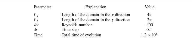
The system of ODEs is numerically integrated using a fourth-order Runge–Kutta scheme with parameters specified in table 1. The temporal evolution of mode coefficients starting from initial condition
 $[0, 0.1, 0.1, 0.1, 0.1, 0, 0, 0, 0]$
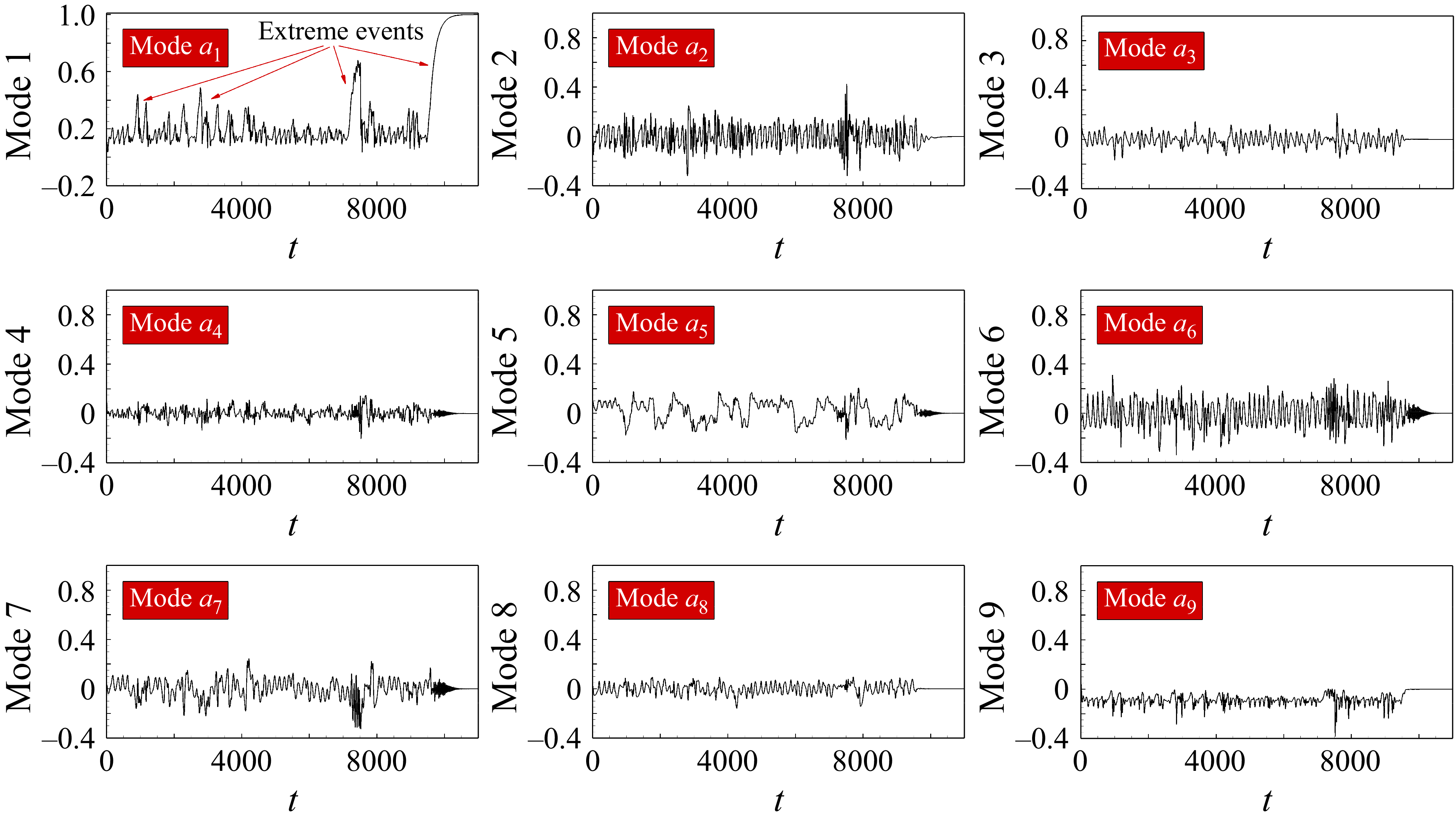
is shown in figure 5, which exhibits chaotic characteristics, eventually converging to a steady-state equilibrium. Throughout the transition phase, intermittent bursts of intense variations are observed. These transient bursts are defined as extreme events (Sapsis Reference Sapsis2021), as shown in figure 6. Due to its simplicity and various turbulence characteristics, including multiscale fluctuations, energy dissipation and relaminarisation, this model has become a benchmark for studying transition (Skufca, Yorke & Eckhardt Reference Skufca, Yorke and Eckhardt2006), turbulence modelling (Srinivasan et al. Reference Srinivasan, Guastoni, Azizpour, Schlatter and Vinuesa2019) and flow control (Racca & Magri Reference Racca and Magri2022).
Parameter settings for the turbulent shear flow model.

Temporal evolution of mode coefficients. Several extreme events burst throughout turbulence evolution. The system ultimately relaxes to a steady-shear-flow state after
 $10^4$
time units.

Instantaneous flow visualisation at
 $t=944$
. (a) Streamline and clipping plane contour. (b) Vortex topology revealed by Q-criterion iso-surfaces.

5.2. Equation-based causal analysis
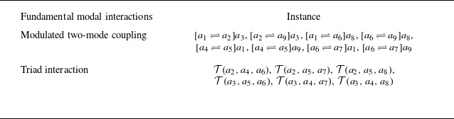
From the mathematical and physical principles of the Galerkin projection (see § 2), we can identify the causal relationships among modes. Inspecting the nonlinear terms in (5.1)–(5.9), the following two types of quadratic modal interactions are identified, and their associated causal relationships can lead to a directed cause-and-effect network of nonlinear dynamics.
-
(i) Modulated two-mode coupling: the mutual interaction of two modes controlled by a third mode whose evolution remains independent of the other two, as illustrated in figure 7(a). For instance, consider the nonlinear interactions among modes 1, 2 and 3. It can be observed that the governing equations of modes 1 and 2 mutually contain quadratic terms with coefficients of opposite signs (i.e.
 $Q_{123}=-Q_{213}$
), while mode 3 lacks terms involving mode 1 or 2 (i.e.
$Q_{321}=0$
). The energy conservation is thus maintained by
$Q_{123}+Q_{213}+Q_{321}=0$
. Therefore, modes 1 and 2 form a transfer pair, with mode 3 acting as a catalyst that facilitates their interaction and energy transfer, defined as the modulator. This phenomenon physically represents a self-sustaining process (Waleffe Reference Waleffe1997) in turbulent shear flow, where streamwise rolls redistribute the mean shear flow to create streaks. Such a relationship is shown in figure 8, denoted as
$[a_1 \rightleftharpoons a_2] a_3$
, with analogous instances including
$[a_1 \rightleftharpoons a_6] a_8$
,
$[a_4 \rightleftharpoons a_5] a_1$
, etc. From the perspective of causality, this interaction consists of four causal relations: a bidirectional causality within the transfer pair and two unidirectional causalities from the modulator to the two pair modes separately.
-
(ii) Triad interaction: the mutual coupling among three modes, where each mode acts as a modulator for the interaction of the other two modes, as illustrated in figure 7(b). In the present model, modes 2, 4 and 6 form a triad interaction, appearing in each other’s governing equations with quadratic term coefficients that strictly sum to zero (
$Q_{246}+Q_{426}+Q_{624}=0$
). This principle governs mutual energy transfer between modes while conserving the total energy (Kraichnan & Chen Reference Kraichnan and Chen1989; Noack et al. Reference Noack, Schlegel, Ahlborn, Mutschke, Morzyński, Comte and Tadmor2008; Loiseau & Brunton Reference Loiseau and Brunton2018). This relationship is denoted as
$\mathcal{T}(a_2, a_4, a_6)$
with analogous instances including
$\mathcal{T}(a_3, a_5, a_6)$
,
$\mathcal{T}(a_3, a_4, a_7)$
etc. Within the triad interaction, each pair of modes exhibits mutual causation, resulting in three bidirectional causalities. Notably, here the causality is defined as the direct cause-and-effect between modes. The absence of such causality does not preclude the possibility of indirect interactions, which may occur through intermediate modes.


Schematic of two types of modal interaction. (a) Modulated two-mode coupling. (b) Triad interaction.

All quadratic interactions identified in the turbulent shear flow model are summarised in table 2, which also leads to a directed causal network shown in figure 9(a) and a causal map shown in figure 9(b). Equation-based causal analysis grounded in rigorous mathematical and physical foundations of the Galerkin model provides reliable insights into causal relationships. However, this approach only provides qualitative results but fails to quantify the magnitude of them. Furthermore, the turbulent shear flow model examined in this study remains simple, i.e. a Fourier-based Galerkin model with sparse and well-structured equations. For complex real-world flows, such an ideal Galerkin model is very difficult to construct, which obscures the application of equation-based analysis in practice. However, empirical Galerkin models using truncated POD bases can also be obtained as the reference model for equation-based analysis, given that the sparse model structure is correctly extracted (Loiseau & Brunton Reference Loiseau and Brunton2018).
Summary of identified modal interactions in turbulent shear flow model.

Interaction between the main shear flow (mode 1) and streaks (mode 2), modulated by the streamwise rolls (mode 3). Three-dimensional mode contours and the temporal evolution of mode coefficients are depicted, illustrating the dynamic interaction between modes.

Equation-based causal network of the turbulent shear flow model. (a) Overall causal links across all modes. Arrow convention: one-way arrows indicate unidirectional causal influence; two-way arrows denote bidirectional causal interactions. (b) Visualised in a
 $9\times 9$
causal map.

5.3. Galerkin-based Granger causality analysis
This section focuses on the identification of causal relationships from data, using the proposed GGC approach. To enhance flow stability, we analyse data generated at a higher Reynolds number
 $Re=600$
, starting from the initial condition [0, 0.1,0.1, 0.1,0.1, 0, 0, 0, 0]. The hyperparameter, i.e. the optimal sampling window, should be determined first. The relationship between CDI and window length is investigated, as illustrated in figure 10. The CDI gradually increases until peaking at around
 $T=400$
, then it gradually declines to a steady value at around
 $T=1000$
. Therefore, the window length is set to 400, corresponding to the maximum CDI value and a clearest causal pattern. It ensures sufficient model accuracy while maximising the cause-and-effect identification among strong causality, weak causality and non-causality.
Determination of the window length, representing the trade-off between time-variant resolution and causal discriminability, where a length of 4000 snapshots (400 time units) yields the optimal outcome.

As shown in figure 11(a), the GGC results provide a quantitative measure of Granger causality. However, to determine which causal interactions actually exist, a binary (0–1) causal map is required. This can be derived from the GGC results using either threshold-based classification or permutation test. In the threshold-based classification, a cutoff value is selected, and causal links with GGC values above this threshold are labelled as ‘true’, while others are labelled ‘false’. A common heuristic is to rank all GGC values and choose the threshold at the ‘elbow’, i.e. the point where the decay curve begins to flatten. For the current problem, this yields a threshold of 0.15, as shown in figure 11(b). Practically, this approach is empirical and relies on expert knowledge. A more rigorous alternative is to apply a permutation test (introduced in § 4). As shown in figure 12, using 100 permutations and a significance level of
 $\alpha =0.1$
, the resulting binary causal map exactly matches the ground-truth causality derived from the governing equations (figure 9). These findings validate the reliability of GGC. Furthermore, using the proposed GGC, one can also identify mode interactions purely from data, if the Galerkin-based model is not available or too complex.
(a) The GGC result of shear flow model; (b) causality ranking and the identification of a threshold value (0.15 in this case), where the decay of GGC shows a tendency of stagnation; (c) binary causal map extracted from permutation test, which is detailed in § 4. The resulting binary causal map shows absolute agreement with equation-based analysis, validating the reliability of GGC.

Permutation tests at different significance levels on the shear flow model (100 permutations). Satisfactory causal identification is achieved for conventional levels 0.05 and 0.1, while misclassifications arise at extreme significance levels.

Based on its definition, the GGC value quantifies the informative contribution of a given mode to the dynamic prediction of other modes. We then take the column-wise sum of outgoing GGC values from each mode as its ‘causal importance’. Physically, it reflects the mode’s overall informative contribution in the system. Notably, its relative ranking and pattern are more meaningful than absolute magnitudes. As shown in figure 14, modes 2 and 6 exhibit the highest score, underscoring their critical roles in the system. This can also be supported by the fact that energy is input through mode 1 (the base profile), and modes 2 (streak) and 6 (normal vortex) play a crucial role in transferring energy from mode 1 to the rest of the system. With this quantification, users can rapidly detect modes that are causally important. The ROMs built from these key modes can capture the essential behaviour of the system, which needs to be modelled with a high level of accuracy.
By varying the initial conditions, Reynolds number and window length, we obtained four sets of data samples. These samples are analysed using GGC, classical Granger causality (implemented with the MVGC toolbox (Barnett & Seth Reference Barnett and Seth2014) without analysis windows), Pearson correlation and transfer entropy (implemented via codes of Martínez-Sánchez et al. (Reference Martínez-Sánchez, López, Le Clainche, Lozano-Durán, Srivastava and Vinuesa2023)) to examine causal relationships between modes. The results are shown in figure 13. We observe significant variations in the results of classical Granger causality across the four datasets, indicating its robustness deficiency. This further demonstrates that the classical Granger causality, as a linear method, is unreliable for discovering causality in nonlinear systems. In contrast, the GGC produced highly consistent results across all datasets, demonstrating strong robustness. This confirms that our modifications to the Granger causality method are both reasonable and effective. Pearson correlation and transfer entropy also yield robust results, but the former reflects only trend similarity (not causality), and the latter recovers fewer causal links than the ground-truth dynamics.
Comparison of GGC, classical Granger causality, Pearson correlation and transfer entropy. (a) Four distinct modal evolution sequences, each corresponding to a unique set of initial conditions and Reynolds numbers. The yellow boxes indicate the windowed sampling used for GGC analysis. (b) The results from the four methods are displayed sequentially (self-causality terms are omitted by definition for causal analysis (GGC/Granger causality/transfer entropy)). The GGC is shown to be the most accurate and robust across all cases.

Finally, GGC is also applicable to complex, high-dimensional flows where a Galerkin-projected model is hard to obtain. As a demonstration, we apply it to analyse the causal structure of a turbulent lid-driven cavity flow (Arbabi & Mezić Reference Arbabi and Mezić2017), which is detailed in Appendix B.
The column sum of the GGC causal map is defined as the causal importance of each mode, representing the total Granger causality exerted by that mode on all other modes.

5.4. Causality-guided flow control
This section demonstrates how causal findings in §§ 5.2 and 5.3 offer valuable insights for flow control. At low Reynolds numbers, extreme events (formulated as strong relaminarisation) emerge in the present turbulent shear flow model. Racca & Magri (Reference Racca and Magri2022) employed echo state networks to predict the evolution of mode coefficients and successfully suppressed extreme events before their onset. Inspired by this work, we approach the same problem from a causal perspective. Specifically, we show that applying control body forces to mode 3 or mode 8 (modulating modes) enables robust suppression of extreme events. The following flow control is conducted at
 $Re=600$
, starting from a random initial condition of
 $[0, 0.03, 0.1, 0.05, 0.1, 0, 0, 0.04, 0]$
.
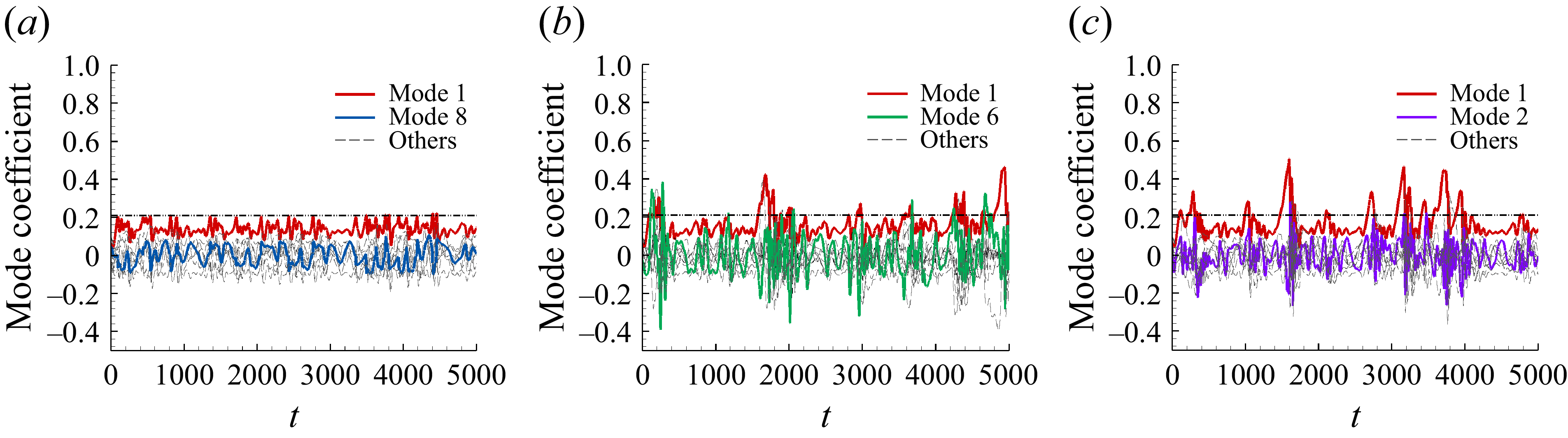
(a) Time evolution of the shear flow mode coefficients, illustrating extreme events as sharp increases in the amplitude of mode 1 (highlighted in yellow). The corresponding flow contours during these events are shown in figure 17(b–d). (b) Binary causal map. Red and blue boxes highlight the modulated two-mode coupling involving modes 1, 2, 3 and modes 1, 6, 8, respectively. In both cases, modes 3 and 8 act as modulators.

As shown in figure 15(a), extreme events are characterised by a sharp increase in the amplitude of mode 1. To suppress such events, it is therefore necessary to extract energy from this mode. As previously introduced in § 5.2, mode 3 acts as a modulator for the energy transfer between modes 1 and 2 (
 $[a_{1}\rightleftharpoons a_{2}]a_{3}$
), and similarly, mode 8 modulates the transfer between modes 1 and 6 (
 $[a_{1}\rightleftharpoons a_{6}]a_{8}$
). These modulating modes (3 and 8) present themselves as the most effective leverage points for extracting energy from mode 1 to mitigate extreme events. Such a conclusion can also be drawn from the data-driven causal map shown in figure 15(b), as modes 2, 3, 6 and 8 are the only ones that cause mode 1. Specifically, modes 2 and 6 engage in a bidirectional interaction with mode 1, whereas modes 3 and 8 exert a unidirectional causal influence on it. This structural pattern suggests that modes 3 and 8 are possible modulators controlling the energy transfer between mode 1 and others.
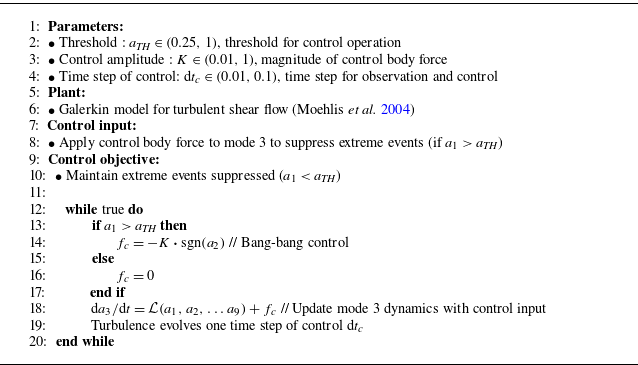
Based on the insights extracted from causal analysis, we can develop a causality-guided flow control strategy: upon detection of an extreme event (
 $a_1\gt a_{\textit{TH}}$
), a control body force is applied to the modulator (mode 3) to facilitate energy transfer from mode 1 to mode 2, thereby suppressing the extreme event. Specifically, to extract energy out of mode 1, the applied body force
 $f_c$
is designed to oppose the instantaneous phase of mode 2. This yields the following expression:
 \begin{align} f_c = \begin{cases} -K \boldsymbol{\cdot }\operatorname {sgn}(a_2), & a_1 \gt a_{\textit{TH}} \\ 0, & a_1 \leqslant a_{\textit{TH}}, \end{cases} \end{align}
where
 $K$
represents the control amplitude and
 $\operatorname {sgn}(\boldsymbol{\cdot })$
denotes the sign function. Since the control amplitude is fixed, it is a typical bang-bang control (Bryson Reference Bryson2018). The complete flow control strategy is presented in Algorithm 1, which is defined by three parameters: threshold
 $a_{\textit{TH}}$
, control amplitude
 $K$
and time step of control
 ${\rm d}t_c$
. We also provide recommended ranges for the three parameters in Algorithm 1.
Suppression of extreme events in shear flow model

With
 ${\rm d}t_c = 0.1$
and
 $K = 0.1$
, the proposed control algorithm effectively suppresses extreme events under various initial conditions and thresholds, as illustrated in figure 16(a–c). Further testing reveals that modifying the time step and control amplitude influences the response speed of the control system, thereby affecting the future evolution of the flow, as shown in figure 16(d,e). Despite these variations, the system remains capable of suppressing extreme events, demonstrating strong robustness. The operating time of the control system is notably brief, minimising both control costs and flow interference. The flow fields before and after suppressing extreme events are depicted in figure 17. It is shown that activation of the control system effectively maintains turbulent structures and suppresses extreme events.
Suppression of extreme events by applying control body force to mode 3 under various conditions. The time step is set to
 ${\rm d}t_c=0.1$
in (a–c), with a control amplitude of
 $K=0.01$
. (a) The case without control, and the results of control thresholds set at (b)
 $a_{\textit{TH}}=0.4$
and (c)
 $a_{\textit{TH}}=0.2$
. In (d),
 ${\rm d}t_c$
is reduced to
 $0.01$
. The control amplitude for (e) is increased to
 $K=0.1$
. Black arrows indicate positions where control is activated.

Snapshots of the flow field during an extreme event (corresponding to figure 16 a,b), comparing uncontrolled (b–d) and controlled (e–g) scenarios. In the uncontrolled case, the flow exhibits a gradual decay towards a laminar shear flow. In contrast, the applied control rapidly suppresses this decay, maintaining turbulent structures and preventing laminarisation.

Having demonstrated the effectiveness of controlling mode 3 to suppress the extreme events, we further apply the same strategy to another modulator (i.e. mode 8). By adding control body force on mode 8, energy is transferred from mode 1 to mode 6. Extreme events are again effectively suppressed, as shown in figure 18(a), indicating the robustness of the proposed causality-guided control. Although both modes 2 and 6 also cause mode 1, control attempts via these modes fail to suppress extreme events, as shown in figure 18(b,c). This failure is attributed to the fact that modes 2 and 6 form the transfer pair with mode 1; therefore they are not directly driving but rather participating in the energy transfer, making them ineffective as control actuators. Even without prior knowledge of the system dynamics, these causal interactions can still be drawn directly from the causal map (figure 15 b). This binary causal map clearly shows that modes 3 and 8 unidirectionally cause mode 1, whereas modes 2 and 6 engage in mutual interaction with it, rendering them less effective in control. These results highlight a key advantage of causal analysis: it not only reveals dynamical mechanisms but also provides valuable insights for control design.
Suppression of extreme events under the same conditions as in figure 16(c), achieved by applying artificial body forces to (a) mode 8, (b) mode 6 and (c) mode 2. Successful suppression is observed only when control is applied to mode 8, which is also a modulating mode.

5.5. Comparisons with other methods
Since standard Granger causality was proposed, numerous nonlinear extensions have been proposed and extensively studied, via incorporating kernels (Marinazzo, Pellicoro & Stramaglia Reference Marinazzo, Pellicoro and Stramaglia2008), radial basis functions (Ancona, Marinazzo & Stramaglia Reference Ancona, Marinazzo and Stramaglia2004), quadratic terms (Lopez-Doriga et al. Reference Lopez-Doriga, Atzori, Vinuesa, Bae, Srivastava and Dawson2024) or even neural networks (Tank et al. Reference Tank, Covert, Foti, Shojaie and Fox2021). While these methods enhance the flexibility by replacing linear autoregression with nonlinear fits, they typically fail to exploit known structural properties of the underlying dynamics. In contrast, GGC is specifically designed for ROMs derived from Navier–Stokes equations. By explicitly embedding this physical structure into the regression model, GGC avoids over-parametrisation and ensures the interpretability aligned with the true dynamics. Furthermore, for non-Granger causality methods, we would especially mention the transfer entropy (Schreiber Reference Schreiber2000) method, which is theoretically equivalent to Granger causality for Gaussian systems (Barnett, Barrett & Seth Reference Barnett, Barrett and Seth2009) and has been successfully applied to fluid systems (Lozano-Durán et al. Reference Lozano-Durán, Bae and Encinar2020; Wang et al. Reference Wang, Lozano-Duran, Helmig and Chu2022; Martínez-Sánchez et al. Reference Martínez-Sánchez, López, Le Clainche, Lozano-Durán, Srivastava and Vinuesa2023; Massaro, Rezaeiravesh & Schlatter Reference Massaro, Rezaeiravesh and Schlatter2023). Generally speaking, transfer entropy is a universal, model-free method with a robust theoretical foundation, demonstrating broader applicability than GGC. However, it relies on the estimation of probability densities, which becomes computationally expensive when encountered with high-dimensional systems (Duan et al. Reference Duan, Yang, Chen and Shah2013) and statistically unreliable when data are limited (Smirnov Reference Smirnov2013). In contrast, GGC is specifically tailored for Galerkin-structured ROMs. It enables reliable causal inference at low computational cost, thereby demonstrating a distinct advantage over transfer entropy in the context of this study.
The causal structure of the shear flow model has also been investigated in recent works using different causal analysis approaches. For instance, Martínez-Sánchez et al. (Reference Martínez-Sánchez, López, Le Clainche, Lozano-Durán, Srivastava and Vinuesa2023) applied transfer entropy, Lopez-Doriga et al. (Reference Lopez-Doriga, Atzori, Vinuesa, Bae, Srivastava and Dawson2024) employed nonlinear Granger causality, while Zhang et al. (Reference Zhang, Zhu, Vinuesa and Hu2024) used a Liang–Kleeman information flow. As shown in figure 19, these methods recover partial causal links but differ in details due to their distinct underlying assumptions. The main contributions of the present paper, compared with previous works, are threefold: (i) data-driven GGC and equation-based analysis are combined to identify causal relations in the shear flow model, resulting in robust, reliable cause-and-effect analysis; (ii) mode interactions are identified by the proposed causal analysis, enhancing the physical interpretations of the underlying mechanisms; and (iii) a causality-guided flow control is presented in this model, through applying control body force to the modulating mode (i.e. the modulator). This type of control successfully suppresses extreme events in the shear flow. Together, these contributions connect equation-based understanding, data-driven causal discovery and flow control, offering guidance for more complex flow problems in future work.
Comparison of various causal analysis methods applied to the shear flow model. The background illustrates results of the GGC. Six significant causal effects, identified by transfer entropy, are marked in green boxes. The causalities uncovered by nonlinear Granger causality are represented by brown circles, with their strength indicated by the size.

6. Conclusions
In this work, we performed causal analysis of a turbulent shear flow developed by Moehlis et al. (Reference Moehlis, Faisst and Eckhardt2004). The analysis helps to characterise nonlinear modal interactions from low-dimensional Galerkin equations and modified Granger causality, named as GGC. The identified two types of quadratic interactions, including a fully triad interaction and a modulated two-mode coupling, as well as the directed cause-and-effect network, offer a causal perspective on the nonlinear flow dynamics and guide the design of flow control strategy.
The proposed GGC is designed for systems following Galerkin-structured dynamics (flow ROMs). It takes modal coefficients as input to formulate a quadratic regression framework and outputs the difference between the prediction with and without the causal mode. Using the GGC, once a mode with large effect is identified, the uncertainties corresponding to the cause mode cannot be ignored. The resulting Granger causal map not only quantifies the cause-and-effect relationships between modes, but also helps identify the quadratic interactions from the equation-based analysis, when transferred to the binary causal map. To assess the applicability of GGC beyond systems with known Galerkin structure, we further apply it to a turbulent lid-driven cavity flow (see Appendix B). Without requiring a pre-existing model, GGC obtains a robust and physically interpretable causal network for the data-driven POD modes. We also show that truncating the system does not significantly alter the inferred causality. These results support GGC as a fully data-driven procedure that allows automated quantification of modal causality.
The proposed causal analysis framework also results in valuable tools for Galerkin modelling, opening promising possibilities in applications of various problems: (i) causal insights may inform reduced-order representation and model-order reduction of nonlinear dynamics (Lassila et al. Reference Lassila, Manzoni, Quarteroni and Rozza2014), or developing improved turbulence closures (Shan & Zhang Reference Shan and Zhang2025); (ii) sensitivity and uncertainty quantification in modal space, potentially offering a variational perspective related to Lyapunov exponents (Oseledec Reference Oseledec1968); and (iii) discovery of the prediction horizon and active subspaces for control design (Bagheri et al. Reference Bagheri, Henningson, Hœpffner and Schmid2009). These aspects will be explored in future works.
Supplementary material
Supplementary material is available at https://doi.org/10.1017/jfm.2026.11553.
Funding
This work was supported by the National Key Research and Development Program of China (2024YFB3310401), the Foundation of National Key Laboratory of Aircraft Configuration Design (JBGS-202,504), the Natural Science Foundation of Shaanxi Province (2025JC-YBQN-087), Science and Technology Plan Project of Shaanxi Province (Grant No. 2024JC-YBQN-0010) and the Fundamental Research Funds for the Central Universities (G2024KY05101).
Declaration of interests
The authors report no conflict of interest.
Data availability statement
The codes and datasets used in this study are available in the following repository: https://github.com/JiaqingKou/Galerkin-based-Granger-Causality.
Appendix A. Mode definition of the turbulent shear flow model
The physical domain of turbulent shear flow is set to
 $0 \leqslant x \leqslant L_x$
,
 $-1 \leqslant y \leqslant 1$
,
 $0 \leqslant z \leqslant L_z$
. Let
 $\alpha = 2\pi / L_x$
,
 $\beta = \pi / 2$
and
 $\gamma = 2\pi / L_z$
. Then the velocity in the turbulent shear flow model (Moehlis et al. Reference Moehlis, Faisst and Eckhardt2004) is projected onto nine Fourier bases (modes), as described below.
The basic profile (shear flow):
 \begin{align} \boldsymbol{u}_1 = \begin{pmatrix} \sqrt {2} \sin (\pi y / 2) \\[3pt] 0 \\[3pt] 0 \end{pmatrix}. \end{align}
The streak:
 \begin{align} \boldsymbol{u}_2 = \begin{pmatrix} \frac {4}{\sqrt {3}} \cos ^2(\pi y / 2) \cos (\gamma z) \\[3pt] 0 \\[3pt] 0 \end{pmatrix}, \end{align}
The downstream vortex:
 \begin{align} \boldsymbol{u}_3 = \frac {2}{\sqrt {4\gamma ^2 + \pi ^2}} \begin{pmatrix} 0 \\[3pt] 2\gamma \cos (\pi y / 2) \cos (\gamma z) \\[3pt] \pi \sin (\pi y / 2) \sin (\gamma z) \end{pmatrix}. \end{align}
The spanwise flows:
 \begin{align} \boldsymbol{u}_4 = \begin{pmatrix} 0 \\[3pt] 0 \\[3pt] \frac {4}{\sqrt {3}} \cos (\alpha x) \cos ^2(\pi y / 2) \end{pmatrix} \end{align}
and
 \begin{align} \boldsymbol{u}_5 = \begin{pmatrix} 0 \\[3pt] 0 \\[3pt] 2 \sin (\alpha x) \sin (\pi y / 2) \end{pmatrix}. \end{align}
The normal vortex modes:
 \begin{align} \boldsymbol{u}_6 = \frac {4\sqrt {2}}{\sqrt {3(\alpha ^2 + \gamma ^2)}} \begin{pmatrix} - \gamma \cos (\alpha x) \cos ^2(\pi y / 2) \sin (\gamma z) \\[3pt] 0 \\[3pt] \alpha \sin (\alpha x) \cos ^2(\pi y / 2) \cos (\gamma z) \end{pmatrix} \end{align}
and
 \begin{align} \boldsymbol{u}_7 = \frac {2\sqrt {2}}{\sqrt {\alpha ^2 + \gamma ^2}} \begin{pmatrix} \gamma \sin (\alpha x) \sin (\pi y / 2) \sin (\gamma z) \\[3pt] 0 \\[3pt] \alpha \cos (\alpha x) \sin (\pi y / 2) \cos (\gamma z) \end{pmatrix}. \end{align}
The fully three-dimensional mode:
 \begin{align} \boldsymbol{u}_8 = \frac {2\sqrt {2}}{\sqrt {(\alpha ^2 + \gamma ^2)(4\alpha ^2 + 4\gamma ^2 + \pi ^2)}} \begin{pmatrix} \pi \alpha \sin (\alpha x) \sin (\pi y / 2) \sin (\gamma z) \\[3pt] 2(\alpha ^2 + \gamma ^2) \cos (\alpha x) \cos (\pi y / 2) \sin (\gamma z) \\[3pt] - \pi \gamma \cos (\alpha x) \sin (\pi y / 2) \cos (\gamma z) \end{pmatrix}. \end{align}
The modification of the basic profile, which is the variation from the eight-mode shear flow model proposed by Waleffe (Reference Waleffe1997):
 \begin{align} \boldsymbol{u}_9 = \begin{pmatrix} \sqrt {2} \sin (3\pi y / 2) \\[3pt] 0 \\[3pt] 0 \end{pmatrix}. \end{align}
Appendix B. Extending GGC to complex problems exemplified by a cavity flow
The proposed GGC framework can be applied to dimensionality reduction techniques (e.g. POD, dynamic mode decomposition or variational autoencoder (Solera-Rico et al. Reference Solera-Rico, Sanmiguel Vila, Gómez-López, Wang, Almashjary, Dawson and Vinuesa2024)) to enable causal analysis in complex high-dimensional flows. Mathematically, this combination yields a truncated Galerkin system, where the dynamics of the low-dimensional mode coefficients is resolved while higher-order dynamics is excluded. In this reduced-order context, GGC can still recover the underlying causal mechanisms governing the flow dynamics, provided that the truncation error is negligible.
To demonstrate this, the two-dimensional post-transient cavity flow data released by Arbabi & Mezić (Reference Arbabi and Mezić2017) are further studied. The flow data are obtained through a Chebyshev spectral collocation simulation of an incompressible lid-driven cavity flow in a square domain [−1, 1]. The Reynolds number is defined as
 $Re = L_c U_c/{\nu } = 2/\nu$
, where
 $L_c=2$
and
 $U_c=1$
are the characteristic length and velocity, respectively. Previous studies report that the flow is periodic at
 $Re=13\,000$
, undergoes a Hopf bifurcation and becomes quasi-periodic at
 $Re=15\,000$
, and transitions to chaos for
 $Re\gt 22\,000$
. More details about this simulation can be found in the literature (Arbabi & Mezić Reference Arbabi and Mezić2017; Arbabi & Mezic Reference Arbabi and Mezic2019).
Snapshot of the lid-driven cavity flow at
 $Re=16\,000$
: (a) vorticity field, (c) velocity magnitude with superimposed vector field and (b) time histories of the velocity components at two selected grid points.

We apply the GGC method to the cavity flow at
 $Re=16\,000$
(figure 20), using the
 $64\times 64$
Chebyshev-grid simulation data from Arbabi & Mezić (Reference Arbabi and Mezić2017). A POD decomposition is first conducted on a dataset comprising
 $10^4$
velocity snapshots with a time interval of 0.1. For the two-component velocity field, POD is applied to the vector field by concatenating the
 $u$
- and
 $v$
-velocity components into a unified snapshot matrix. The first 10 modes take up 71 % of the total energy, capturing the dominant structures of the flow. The resulting POD modes and coefficients are shown in figure 21. A fast Fourier transformation is also conducted on the mode coefficients, which shows that modes 1–4 are dominated by frequencies
 $St=0.155$
and
 $St=0.252$
, modes 5–6 are dominated by a single frequency
 $St=0.097$
, while modes 7–10 exhibit a mixture of frequencies at
 $St=0.194$
,
 $St=0.349$
and
 $St=0.408$
. The basic frequency vector of the cavity flow at
 $Re=16\,000$
is reported as
 $St=[0.155, 0.097]$
(Arbabi & Mezić Reference Arbabi and Mezić2017), while the dominant frequencies of the first 10 POD modes are linear combinations of those two basic flow frequencies.
(a) Contours of the first 10 velocity POD modes for the lid-driven cavity flow at
 $Re=16\,000$
, with colour indicating velocity magnitude and black arrows depicting the velocity vectors. (b) The temporal coefficients of the first 10 POD modes.

The GGC is then applied to infer causal relationships between the first 10 POD modes. To determine the window length, a variety of window lengths are tested, where the corresponding GGC results and CDI values are shown in figure 22. Similar to the shear flow model, the GGC result and CDI value converge as analysis window length increases, and are stabilised beyond 5000 snapshots (
 $T=500$
). This determines an optimal window length of 5000 snapshots, which gives a clear causal structure in figure 22. Furthermore, this convergence behaviour is robust across different numbers of modes considered. A key observation is that the window length required for GGC convergence scales with the number of modes, implying that more data are needed to reliably estimate causality in higher-dimensional systems. Permutation test (introduced in § 4) indicates that statistically significant causalities exist among almost all modes. This is reasonable since they are indeed highly coupled. Notably, the strongest causal links occur between conjugate mode pairs (e.g. modes
 $1\rightleftharpoons 2$
,
 $3\rightleftharpoons 4$
, etc.).
Convergence of the CDI as a function of analysis window length (in snapshots) for GGC analyses using the first 4, 10, 20, 30 and 40 POD modes. In the case of 10 modes, the outcome stabilises beyond 5000 snapshots (
 $T=500$
). This convergence becomes slower as the number of modes increases, indicating a need for longer windows in higher-dimensional analyses.

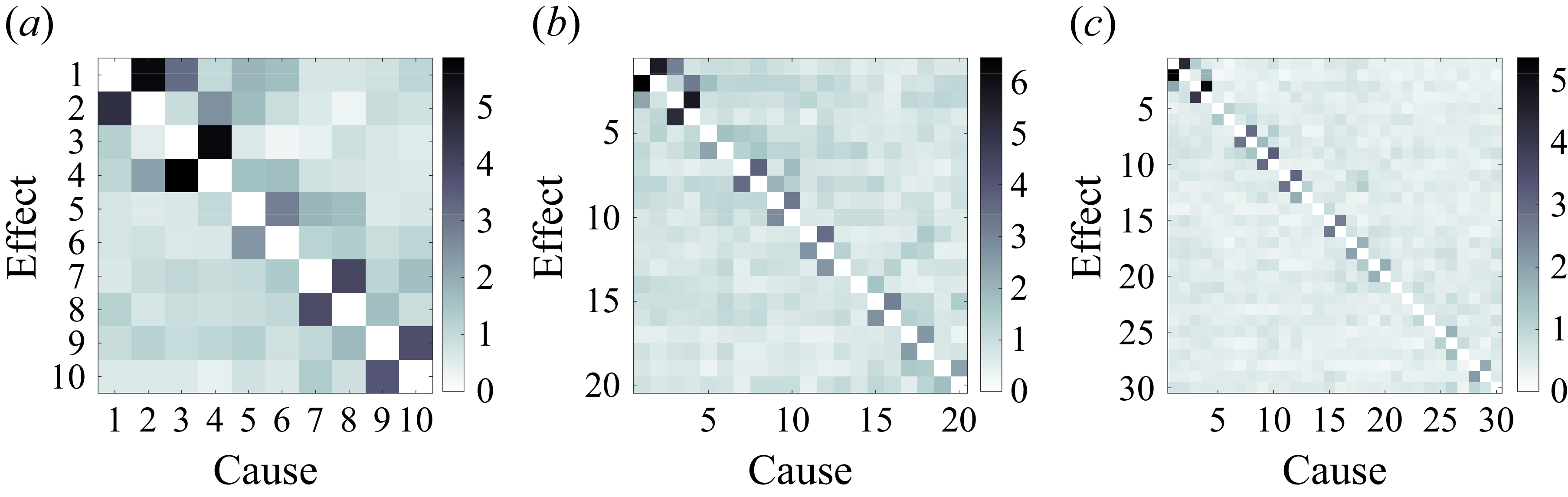
The GGC maps computed using models constructed from (a) 10, (b) 20 and (c) 30 modes. The consistent causal structure of dominant modes across all cases indicates that the results are robust to the inclusion of higher-order modes, supporting the use of GGC on reduced-order systems.

One of the key assumptions underlying Granger causality is a fully observed system, which requires no unmeasured confounders (Shojaie & Fox Reference Shojaie and Fox2022). Since GGC is essentially a Granger causality test applied to a low-dimensional Galerkin model, a natural concern is whether truncating the model by excluding higher-order POD modes may bias the causal inference. To address this, we performed sensitivity analyses on models constructed with varying numbers of POD modes (figure 23). The results reveal that the causal structure among the first 10 modes remains highly consistent across analyses involving 10, 20 and 30 modes. This suggests that the exclusion of higher-order dynamics does not significantly compromise the inferred causal relationships among the dominant modes, which can be attributed to the localised nature of the dynamics. As figure 23 clearly illustrates, strong causal links only exist between neighbouring modes, while the couplings between lower-order and higher-order modes are weak or negligible. However, this approximation may not hold for all flow configurations. For cases where outcomes are sensitive to mode truncation, potential solutions include increasing the number of modes preserved, or extending the GGC framework with higher-order nonlinearity to model the effect of truncated modes (Noack et al. Reference Noack, Afanasiev, Morzyński, Tadmor and Thiele2003; Loiseau & Brunton Reference Loiseau and Brunton2018).
A GGC analysis to the cavity flow at
 $Re = 30,000$
is further provided in the supplementary material. These support the validity of GGC on more complicated flow problems. A deep physical interpretation of the above causal observations lies beyond the scope of the present work, while future works may investigate the underlying mechanisms of these results.