
I. INTRODUCTION
Despite ever increasing computational powers, modeling and simulation of complex materials at the atomic level—the subject of this Focus Issue—still remains a formidable challenge.Reference Lu, Kaxiras, Rieth and Schommers1 On the one hand, quantum mechanics (QM) is indispensable for a proper treatment of bond-breaking, charge transfer, electron excitation, magnetism, etc., in materials. However, QM calculations are often so expensive that no more than a few hundred atoms can be handled routinely. On the other hand, atomistic simulations based on empirical interatomic potentials, termed molecular mechanical (MM) methods, are capable of describing small-amplitude vibrations and torsions, elastic deformation, electrostatic interactions, etc., in many material problems; these empirical MM methods can treat millions or more atoms in routine calculations. The coupled quantum mechanics/molecular mechanics (QM/MM) methods by combining the accuracy of the QM description with the low computational cost of MM modeling can thus offer a promising solution to the computational challenge in atomistic simulations of materials. In recent years, significant progress has been made in the development of QM/MM methodologies and the application of these methods in atomistic simulations of materials.Reference Abraham, Bernstein, Broughton and Hess2–Reference Peng, Zhang, Huang, Carter and Lu23 There are generally two categories of QM/MM methods applicable to two different classes of materials. In materials where covalent bonds are dominant (organic and inorganic semiconductors, molecular materials, etc.), one can partition the system by cutting the covalent bonds linking the QM and MM parts and then saturate the dangling bonds at the boundary of the QM region by the so-called link atoms.Reference Lin and Truhlar17–Reference Gao and Truhlar19 This and similar procedures can be justified thanks to the presence of localized covalent bonds in such materials. However, for metallic materials, these procedures are no longer valid because of the delocalized nature of metallic bonding; it becomes impractical or impossible to cut and saturate metallic bonds. In fact, the very concept of bonds becomes less appropriate than the band picture for metals. Therefore, different ideas are needed to deal with metallic cohesion represented by the delocalized electron states across the QM/MM boundary. In this paper, we focus on the second category of QM/MM methods and review two recent advances on QM/MM modeling of metallic materials: (i) charge density embedding based on orbital-free (OF) density functional theoryReference Zhang and Lu20,Reference Zhang, Wang and Lu21 ; (ii) charge density embedding based on constrained density functional theory.Reference Zhang, Lu and Curtin22 The extension of QM/MM coupling to multiscale quasicontinuum (QC) method is also highlighted, which offers a route toward quantum mechanical simulations of materials at micron scales and beyond.Reference Peng, Zhang, Huang, Carter and Lu23 The theoretical formulation and applications of the QM/MM methods are discussed in detail. We close with a brief summary and outlook on future development of QM/MM modeling for metals.
II. QM/MM METHODOLOGY
In a QM/MM simulation, the entire system is partitioned into two spatial regions of a material. Region I usually constitutes a much smaller portion of the computational domain where the QM description is crucial to capture and elucidate the material properties. Region II constitutes a much larger computational domain where the classical MM description is sufficient to account for the underlying material problems. Although different levels of QM simulations could be used in region I, here, we focus on the Kohn–Sham density functional theory (KS-DFT).Reference Kohn and Sham24 Similarly, although many empirical potentials could be used in region II, we choose the embedded-atom method (EAM)Reference Daw and Baskes25 as an example for MM calculations in this paper. In general, the total energy of a QM/MM system can be expressed in the following, including the energy of region I in the absence of region II, the energy of region II in the absence of region I, and the interaction energy between the two regions:
 $${E_{{\rm{tot}}}}\left[ {{\rm{I}} + {\rm{II}}} \right] = {E_{{\rm{DFT}}}}\left[ {\rm{I}} \right] + {E^{{\mathop{\rm int}} }}\left[ {{\rm{I}},{\rm{II}}} \right] + {E_{{\rm{MM}}}}\left[ {{\rm{II}}} \right]\quad .$$
The all-important QM contribution is mostly contained in the first term, which appears to require some type of DFT cluster calculations. This, however, could lead to significant errors, which stem from the missing electronic interaction at the cluster surface extending into the interior of region I. Therefore, a successful QM/MM method should restore the missing electronic interaction between regions I and II. Indeed, the crux of QM/MM modeling lies in its handling of the interaction energy, E int[I, II]. The goal of the QM/MM methods is thus to determine E int[I, II] with the same accuracy as would be obtained if the region II were fully quantum mechanical. This goal can be achieved by the so-called quantum mechanical coupling in which E int[I, II] is formulated based on DFT. In other words, the QM calculation of region I is carried out in the presence of region II, whose effect is captured by a single-particle embedding potential that enters the KS Hamiltonian of region I. In the following, we discuss two recently developed QM/MM methods based on the QM coupling. In the first method,Reference Zhang and Lu20,Reference Zhang, Wang and Lu21 the embedding potential is formulated by the OFDFT,Reference Garcia-Gonzalez, Alvarellos and Chacon26–Reference Shin and Carter30 while the second methodReference Zhang, Lu and Curtin22 employs the concept of constrained DFTReference Zhao and Parr31–Reference Wu and Yang33 to determine the embedding potential at the KS-DFT level.
A. Charge density embedding based on OFDFT
1. Basic idea
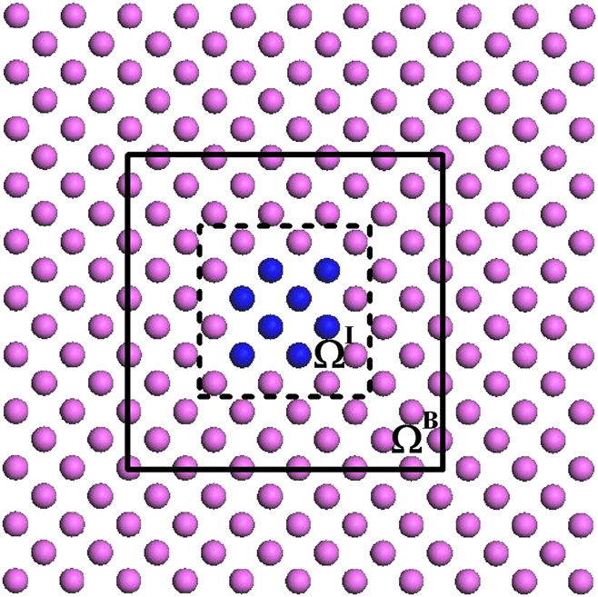
In the first QM/MM method, the interaction energy and the embedding potential are self-consistently determined based on OFDFT. The spatial partition of the entire system is shown in Fig. 1. In specific, the total energy is written asReference Zhang and Lu20
 $${E_{{\rm{tot}}}}\left[ {{\rho ^{{\rm{tot}}}};{{\bf{R}}^{{\rm{tot}}}}} \right] = \mathop {\min }\limits_{{\rho ^{\rm I}}} \left\{ {{E_{{\rm{KS}}}}\left[ {{\rho ^{\rm I}};{{\bf{R}}^{\rm I}}} \right] + E_{{\rm{OF}}}^{{\mathop{\rm int}} }\left[ {{\rho ^{\rm I}},{\rho ^{{\rm I}{\rm I}}};{{\bf{R}}^{\rm I}},{{\bf{R}}^{{\rm I}{\rm I}}}} \right]} \right\} + {E_{{\rm{MM}}}}\left[ {{{\bf{R}}^{{\rm I}{\rm I}}}} \right]\quad ,$$
where Rtot ≡ RI ∪ RII, RI and RII denote atomic coordinates in regions I and II, respectively. The charge density of region I, ρI, which is the degree of the freedom of the problem, is determined self-consistently by minimizing the total energy functional Eq. (2). Each MM atom in region II is associated with an atomic-centered electron density (ρat) and a pseudopotential; both of them are constructed a priori and remain fixed during a QM/MM simulation. The charge density of region II, ρII, is defined as a superposition of atomic-centered charge densities ρat via 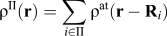 ${\rho ^{{\rm{II}}}}\left( {\bf{r}} \right) = \sum\limits_{i \in {\rm{II}}} {{\rho ^{{\rm{at}}}}\left( {{\bf{r}} - {{\bf{R}}_i}} \right)}$, which only changes upon the relaxation of region II ions. The total charge density ρtot is given by ρtot = ρI + ρII. The interaction energy between regions I and II,
 $E_{{\rm{OF}}}^{{\mathop{\rm int}} }$, formulated by OFDFT is defined as followsReference Zhang and Lu20:
 $$E_{{\rm{OF}}}^{{\mathop{\rm int}} }\left[ {{\rho ^{\rm{I}}},{\rho ^{{\rm{II}}}};{{\bf{R}}^{\rm I}},{{\bf{R}}^{{\rm I}{\rm I}}}} \right] = {E_{{\rm{OF}}}}\left[ {{\rho ^{{\rm{tot}}}};{{\bf{R}}^{{\rm{tot}}}}} \right] - {E_{{\rm{OF}}}}\left[ {{\rho ^{\rm I}};{{\bf{R}}^{\rm I}}} \right] - {E_{{\rm{OF}}}}\left[ {{\rho ^{{\rm I}{\rm I}}};{{\bf{R}}^{{\rm I}{\rm I}}}} \right]\quad .$$
The schematic diagram of the partitioned QM/MM system. Blue and magenta spheres represent the atoms belonging to region I and region II, respectively. The dashed box represents ΩI, and the solid box represents the periodic box ΩB used for the evaluation of the kernel terms of the interaction energy. From Zhang et al.Reference Zhang and Lu20

The OFDFT enables a QM calculation of energetics by knowing only the electronic density. The accuracy of OFDFT is in between KS-DFT and EAM, which is consistent to its usage in the QM/MM method.
The plane-wave pseudopotential methodReference Kresse and Furthmuller34,Reference Kresse and Furthmuller35 is used for the KS-DFT simulation of region I. The KS-DFT total energy functional, E KS[ρI; RI], appearing in Eq. (2) is written asReference Kresse and Furthmuller34
 $${E_{{\rm{KS}}}}\left[ {\left\{ \phi \right\};\left\{ {\bf{R}} \right\}} \right] = \sum\limits_n {{f_n}\left\langle {{\phi _n}\left| {T + V_{{\rm{NL}}}^{{\rm{ion}}}} \right|{\phi _n}} \right\rangle } + {E_{\rm{H}}}\left[ \rho \right] + {E_{{\rm{XC}}}}\left[ \rho \right] + \int {{\rm{d}}{\bf{r}}V_{{\rm{loc}}}^{{\rm{ion}}}\left( {\bf{r}} \right)\rho \left( {\bf{r}} \right)} + {\gamma _{{\rm{Ewald}}}}\left( {\left\{ {\bf{R}} \right\}} \right)\quad ,$$
where n is the index of KS orbitals ϕn and f n is the occupation number. R denotes the position of the ions. k index in reciprocal space is dropped for simplicity. E H and E XC are the Hartree energy and the exchange–correlation energy, respectively.  $V_{{\rm{loc}}}^{{\rm{ion}}}$ and
 $V_{{\rm{NL}}}^{{\rm{ion}}}$ are the local and nonlocal parts of the ionic pseudopotential, respectively, and γEwald is the Madelung energy. A similar expression can be written for OFDFT energy functional E OF as in Eq. (2), in which the electron density instead of the KS orbitals is the degree of freedom. In other words, the OFDFT energy can be expressed as an explicit functional of electron densityReference Garcia-Gonzalez, Alvarellos and Chacon26–Reference Shin and Carter30
 $${E_{{\rm{OF}}}}\left[ {\rho ;{\bf{R}}} \right] = {T_{{\rm{TF}}}}\left[ \rho \right] + {T_{{\rm{vW}}}}\left[ \rho \right] + {T_{\ker }}\left[ \rho \right] + {E_{\rm{H}}}\left[ \rho \right] + {E_{{\rm{XC}}}}\left[ \rho \right] + \int {{\rm{d}}{\bf{r}}V_{{\rm{loc}}}^{{\rm{ion}}}\left( {\bf{r}} \right)\rho \left( {\bf{r}} \right)} + {\gamma _{{\rm{Ewald}}}}\left( {\left\{ {\bf{R}} \right\}} \right)\quad ,$$
where T TF is the Thomas–Fermi contribution which is exact for a uniform electron gasReference Thomas36,Reference Fermi37 ; T vW is the von Weizsacher term which is exact for a single electron orbitalReference von Weizsacker38; and T ker is a density-dependent convolution term to ensure the correct linear-response of the electron gas.Reference Wang, Govind and Carter28 The three terms together represent an approximation to the exact noninteracting kinetic energy.
The minimization of total QM/MM energy [Eq. (2)] with respect to ρI leads to a self-consistent solution of the KS-like eigenvalue equationsReference Zhang and Lu20
 $${\bf{H}}\left| {{\varphi _n}} \right\rangle = \left( {T + {V_{{\rm{loc}}}} + {V_{{\rm{NL}}}}} \right)\left| {{\varphi _n}} \right\rangle = {\varepsilon _n}{\bf{S}}\left| {{\varphi _n}} \right\rangle \quad ,$$
where S is the overlapping matrix with the orthonormalization constraints of the KS orbitals 〈φn|S|φm〉 = δnm, and
 $${V_{{\rm{loc}}}} = V_{{\rm{loc}}}^{{\rm{ion}}}\left[ {{{\bf{R}}^{\rm I}}} \right] + {V_{\rm{H}}}\left[ {{\rho ^{\rm I}}} \right] + {V_{{\rm{XC}}}}\left[ {{\rho ^{\rm I}}} \right] + {\mu _{{\rm{emb}}}}\left[ {{\rho ^{\rm I}},{\rho ^{{\rm I}{\rm I}}}} \right]\quad ,$$
where V H[ρ] and V XC[ρ] are the Hartree potential and the exchange–correlation potential, respectively. µemb[ρI, ρII] is termed embedding potential, which is defined as a functional derivative of the interaction energy  $E_{{\rm{OF}}}^{{\mathop{\rm int}} }$ with respect to ρI,
 $${\mu _{{\rm{emb}}}}\left( {\bf{r}} \right) \equiv {{\delta E_{{\rm{OF}}}^{{\mathop{\rm int}} }\left[ {{\rho ^{\rm I}},{\rho ^{{\rm I}{\rm I}}};{{\bf{R}}^{\rm I}},{{\bf{R}}^{{\rm I}{\rm I}}}} \right]} \over {\delta {\rho ^{\rm I}}}}\quad ,$$
where µemb(r) represents the effective single-particle potential that region I electrons experience due to the presence of both electrons and ions of region II atoms. The QM/MM coupling is achieved by incorporating the embedding potential in the generalized KS equation; both µemb(r) and KS equations have to be solved self-consistently. The nonlocal potential V NL depends on the total local potential V loc.Reference Kresse and Furthmuller34,Reference Kresse and Furthmuller35 For a given charge density ρI, one can determine the band-structure energy εn and the KS orbital φn from the KS eigenvalue Eq. (6). And the total energy of Eq. (2) is calculated byReference Zhang and Lu20
 $${E_{{\rm{tot}}}} = \sum\limits_n {{f_n}{\varepsilon _n}} + {E_{{\rm{d}}{\rm{.c}}{\rm{.}}}} + {\gamma _{{\rm{Ewald}}}}\left[ {{{\bf{R}}^{\rm I}}} \right] + {E_{{\rm{MM}}}}\left[ {{{\bf{R}}^{{\rm I}{\rm I}}}} \right]\quad .$$
The double-counting energy term E d.c. is given by
 $${E_{{\rm{d}}{\rm{.c}}{\rm{.}}}} = - {E_{\rm{H}}}\left[ {{\rho ^{\rm I}}} \right] + {E_{{\rm{XC}}}}\left[ {{\rho ^{\rm I}}} \right] - \int {d{\bf{r}}} {V_{{\rm{XC}}}}\left( {\bf{r}} \right){\rho ^{\rm I}}\left( {\bf{r}} \right) + E_{{\rm{OF}}}^{{\mathop{\rm int}} }\left[ {{\rho ^{\rm I}},{\rho ^{{\rm I}{\rm I}}};{{\bf{R}}^{\rm I}},{{\bf{R}}^{{\rm I}{\rm I}}}} \right] - \int {{\rm{d}}{\bf{r}}{\mu _{{\rm{emb}}}}\left( {\bf{r}} \right)} {\rho ^{\rm I}}\left( {\bf{r}} \right)\quad .$$
Then, ρI and E tot can be self-consistently determined for a given ionic configuration.
2. Implementation and parameterization
Next, we provide a brief discussion on how key calculations from Eqs. (6) to (10) are carried out. In the plane-wave basis, the Hamiltonian H(k) in Eq. (6) is constructed in the reciprocal space as a function of k. The Hartree potential V H(G) and the local pseudopotential V ionloc(G) in Eq. (7) are calculated in the reciprocal space,Reference Martin39 and G is the reciprocal lattice vector. The exchange–correlation potential V XC and the embedding potential µemb are evaluated in the real space first and are then transformed into the reciprocal space by fast Fourier transform (FFT). Once the Hamiltonian is constructed, Eq. (6) is solved in the reciprocal space. With the ground state KS orbitals, KS eigenvalues, and the electron density, the total energy can be evaluated accordingly.
In the KS-DFT plane-wave calculation of region I, we introduce a periodic box ΩB as shown in Fig. 1 over which the periodic boundary conditions (PBCs) are imposed. The PBCs are necessary for FFTs, which are crucial for efficient numerical calculations. In the following, we justify the use of the PBCs with the realization that the real QM/MM system is nonperiodic. In a QM/MM simulation, there exist MM ions and charge density (i.e., no vacuum) beyond ΩI. However, we employ the plane-wave DFT method to calculate the QM charge density which needs a periodic supercell (ΩB). The justification is analogous to the slab model used for surface calculations with the PBCs. In the slab model, the wave-function and the electron density of the surface are assumed to decay exponentially so that they are vanishing at the end of the vacuum slab. Therefore, the PBCs do not lead to appreciable errors. In the case of QM/MM, the basic ansatz is that ρI is confined within ΩI so that the wave function and the charge density of region I decay to zero beyond ΩI. Thus, all the QM/MM interactions are captured within ΩI, and the vacuum introduced between ΩI and ΩB merely serves the purpose to eliminate the spurious interaction among the periodic images in the DFT calculations. As long as the vacuum is large enough, the spurious interaction can be effectively eliminated. Note that although the PBCs are used in the present QM/MM method, the presence of MM region provides much more realistic (both the atomistic and electronic) boundary conditions than a stand-alone periodic DFT calculation. Therefore, the QM/MM method is particularly useful for treating the extended defects, such as dislocations. Since ρII is a key quantity for an accurate evaluation of the interaction energy and the embedding potential, it is crucial to construct an appropriate ρII. In fact, constructing an appropriate charge density in the MM region is a common challenge to many QM/MM methods.Reference Lin and Truhlar17 ρII is defined as a superposition of spherical atomic-like charge densities ρat centered on each ion in region II, which is a reasonable approximation for metallic systems. Ideally, the superposition of ρat (r − Ri) should reproduce the true DFT charge density ρbulk in the perfect bulk. We thus determine ρat by introducing and minimizing an objective function I, defined as the square of the difference between the target density and the true bulk density integrated over a unit cell of the perfect lattice, with respect to variational parameters. The objective function I is given byReference Zhang and Lu20
 $$I = {\int_V {\left[ {\sum\limits_i {{\rho ^{{\rm{at}}}}\left( {{\bf{r}} - {{\bf{R}}_i}} \right)} - {\rho _{{\rm{bulk}}}}\left( {\bf{r}} \right)} \right]} ^2}{\rm{d}}{\bf{r}}\quad ,$$
where V represents the volume of the unit cell and the sum includes all ions in a perfect crystal. The atomic-like charge density is constructed from Gaussian-type orbitals as
 $${\rho ^{{\rm{at}}}}\left( {\bf{r}} \right) = \sum\limits_{lm} {{c_{lm}}{{\left| {{R_l}\left( r \right){Y_{lm}}\left( {\theta ,\phi } \right)} \right|}^2}} \quad ,$$
where {r, θ, ϕ} are spherical coordinates, and l and m are angular and magnetic quantum numbers. c lm are coefficients ensuring that  $\sum\limits_{lm} {{c_{lm}}}$ equals the number of valence electrons of the atom. Y lm are spherical harmonics, and the radial functions R l are Gaussian functions given by R l(r) = r lA(l, αlm)exp(−αlmr 2). A(l, αlm) are normalization factors. The parameters c lm and αlm are determined by minimizing I.
Finally, we consider the ionic forces in the present QM/MM method, which are calculated by taking the derivative of the total energy with respect to ionic displacement. In the ground state, the ionic forces in region I (Fi∈I) and region II (Fi∈II) can be written asReference Zhang and Lu20
 $$\matrix{ { - {{\bf{F}}_{i \in {\rm I}}} = {{\partial {E_{{\rm{KS}}}}\left[ {\rm I} \right]} \over {\partial {{\bf{R}}_i}}} + {{\partial E_{{\rm{OF}}}^{{\mathop{\rm int}} }} \over {\partial {{\bf{R}}_i}}}} \cr { - {{\bf{F}}_{j \in {\rm I}{\rm I}}} = {{\partial E_{{\rm{OF}}}^{{\mathop{\rm int}} }} \over {\partial {{\bf{R}}_j}}} + {{\partial {E_{{\rm{MM}}}}\left[ {{\rm I}{\rm I}} \right]} \over {\partial {{\bf{R}}_j}}}} \cr} \quad .$$
For the evaluation of Fi∈II, there is a disparity in the energetic formulation of  $E_{{\rm{OF}}}^{{\mathop{\rm int}} }$ and E MM. This disparity in turn leads to a disparity in the force formulation, which causes coupling errors in the ionic force, or “ghost force”.Reference E, Lu and Yang40–Reference Liu, Lu, Chen and Kioussis42 To eliminate the coupling errors, we introduce a correction scheme, similar to Ref. Reference E, Lu and Yang40. In this scheme, we require that the ionic force in region II be identical to that derived from an EAM calculation for the entire system, i.e.,
 ${\bf{F}}_{i \in {\rm{{\rm I}I}}}^ * = - \partial {E_{{\rm{MM}}}}\left[ {{\rm I} + {\rm{II}}} \right]{\rm{/}}\partial {{\bf{R}}_i}$. To meet this requirement, a correction force
 $\Delta {\bf{F}}_{i \in {\rm I}{\rm I}}^{{\rm{corr}}}$ is introduced asReference Zhang and Lu20
 $$\Delta {\bf{F}}_{i \in {\rm I}{\rm I}}^{{\rm{corr}}} = {\bf{F}}_i^ * - {{\bf{F}}_i} = {{\partial \left( {E_{{\rm{OF}}}^{{\mathop{\rm int}} } - E_{{\rm{EAM}}}^{{\mathop{\rm int}} }} \right)} \over {\partial {{\bf{R}}_i}}}\quad ,$$
and will be added to the original expression of Eq. (13). Similarly, the disparity could also lead to coupling errors on the ionic forces in region I. Since  ${\bf{F}}_{i \in {\rm{I}}}^{{\mathop{\rm int}} }$ is short-ranged, it is nonzero only on the ions at the QM/MM boundary.Reference Zhang and Lu20 Therefore, the coupling errors would only be present on these ions. Hence, we can employ the same correction scheme as described above. Finally, to ensure the consistency between the total energy and the ionic forces, we introduce a correction to the total energy as wellReference Zhang and Lu20:
 $$E_{{\rm{tot}}}^ * = {E_{{\rm{tot}}}} - \sum\limits_i {\Delta {\bf{F}}_i^{{\rm{corr}}} \cdot \Delta {{\bf{R}}_i}} \quad ,$$
where i signifies the ion with nonzero correction force, ΔRi is its displacement during the relaxation, and the last term represents the work done by the correction force. This scheme has been shown to restore the consistence between total energy and ionic forces, which significantly reduces the coupling errors.Reference Zhang and Lu20,Reference E, Lu and Yang40–Reference Liu, Lu, Chen and Kioussis42
B. Quantum coupling based on constrained DFT
1. Basic idea
The accuracy of the first QM/MM approach relies on the approximate kinetic energy functional and local pseudopotential in the OFDFT formulation. However, despite the recent progress in the development of OFDFT, it remains less accurate than KS-DFT in general. To circumvent the deficiencies of OFDFT, we have developed a QM/MM approachReference Zhang, Lu and Curtin22 based on the constrained DFTReference Zhao and Parr31–Reference Wu and Yang33 that does not invoke OFDFT approximation and thus can be applied to a much broader range of metallic materials.
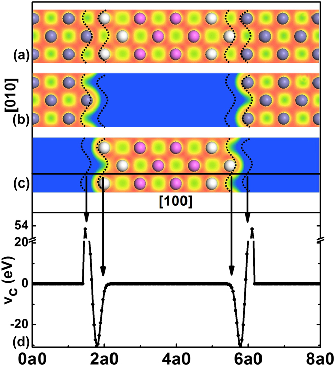
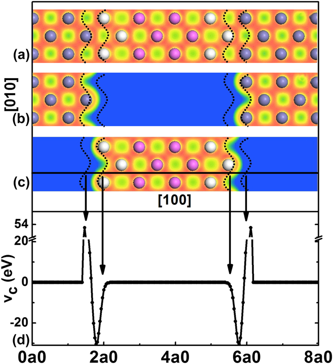
The basic assumption of the constrained DFT-based QM/MM method is that the MM region (region II) is defect-free but could experience small elastic deformations; large lattice deformations and significant electron redistribution are contained only in the QM region (region I). The region I is then partitioned into two spatial domains labeled Ii, and Ib, respectively, as shown schematically in Fig. 2. The inner QM region Ii involves chemical reaction, charge transfer, and bond breaking/formation, etc., thus requiring quantum treatment. The outer MM region II involves small elastic deformations and so can be treated using atomistic interatomic potentials (or continuum mechanics via finite elements). QM region Ib exists between the regions Ii and II and serves as a boundary region that couples regions Ii and II; it must be similar to region II with no defects and relatively small deformations. The selection of region Ib must ensure that (i) there is no direct electronic bonding between regions Ii and II and (ii) the separation between regions Ii and II is greater than the interatomic potential cutoff distance. Hence, regions Ii and II only interact through region Ib. Typically, region II includes two atomic layers of ions as shown in Fig. 2.
The entire system (a) is partitioned into subsystems (b) and (c) in terms of both ions and electron densities. The magenta, white, and gray spheres represent the ions belonging to regions Ii, Ib, and II, respectively. The dashed curves outline the boundaries of Ωc in the (001) plane. The density contour scales (in Å−3) range from 0.0 (blue) to 0.24 (red). (d) The constraint potential is plotted along a straight line in the [100] direction for a perfect lattice; the straight line is indicated in (c). All these results are obtained by λ = 20 for Al. From Zhang et al.Reference Zhang, Lu and Curtin22
We can formally write the total energy of the entire system as
 $${E_{{\rm{tot}}}}\left[ {{{\rm{I}}_{\rm{i}}} + {{\rm{I}}_{\rm{b}}} + {\rm{II}}} \right] = E\left[ {{{\rm{I}}_{\rm{i}}} + {{\rm{I}}_{\rm{b}}}} \right] + E\left[ {{{\rm{I}}_{\rm{b}}} + {\rm{II}}} \right] - E\left[ {{{\rm{I}}_{\rm{b}}}} \right]\quad .$$
Now, we specify that the energy E[Ii + Ib] will be computed using a DFT method, E[Ii + Ib] = E DFT[Ii + Ib], and that the energy E[Ib + II] will be computed using a MM method, E[Ib + II] = E MM[Ib + II]. The remaining energy E[Ib], subtracted out so as to avoid “double counting” of the energy of region Ib, can be computed by either DFT or MM. Here, we compute E[Ib] using MM, E[Ib] = E MM[Ib], so that the total energy retains QM energies from both regions Ii and Ib, i.e., the entire QM region I. The QM/MM method then yields an estimate for the total energy of the entire system asReference Zhang, Lu and Curtin22
 $${E_{{\rm{tot}}}}\left[ {{{\rm{I}}_{\rm{i}}} + {{\rm{I}}_{\rm{b}}} + {\rm{II}}} \right] = {E_{{\rm{DFT}}}}\left[ {{{\rm{I}}_{\rm{i}}} + {{\rm{I}}_{\rm{b}}}} \right] + {E_{{\rm{MM}}}}\left[ {{{\rm{I}}_{\rm{b}}} + {\rm{II}}} \right] - {E_{{\rm{MM}}}}\left[ {{{\rm{I}}_{\rm{b}}}} \right]\quad .$$
Usually, a standard cluster computation of E DFT[Ii + Ib] would lead to relaxation of the electronic degrees of freedom near the outer surface of the computational domain (i.e., in region Ib) and propagation of density fluctuations (Friedel oscillations) deep into region Ii. Here, we use constrained DFT to compute E DFT[Ii + Ib], where the DFT cluster calculation is constrained to have, in principle, the exact correct electronic charge density at the outer boundary of region Ib. Since the charge density in this region is accurate, there are no Friedel oscillations and no spurious forces are generated in region Ii.
2. Implementation and parameterization
Now, we specify how the constrained DFT is used to compute DFT energy of region I. The total electron density is decomposed into contributions associated with the QM ions in regions Ii + Ib and the MM ions in region II, ρtot = ρQM + ρMM. The two electron densities ρQM and ρMM are not confined to their own spatial domains, i.e., ρQM extends into the MM region and vice versa. Thus, a domain Ωc is defined by the overlapping QM and MM charge densities, which straddles regions Ib and II, as shown in Fig. 2. Because there is no direct electronic bonding between regions Ii and II, the electron density from ions in region Ii is required to be zero in Ωc to avoid overlap with ρMM. Thus, ρQM (r ∈ Ωc) is due solely to electrons associated with the ions in region Ib.
Since regions Ib and II are similar to a perfect crystal, their electron densities should be bulk-like and can thus be well represented by a superposition of atomic charge densities, determined a priori for each ionic species. More specifically, the MM charge density is computed as the sum of atomic charge densities ρat (r − Ri) centered at each MM ion Ri,  ${\rho ^{{\rm{MM}}}}\left( {\bf{r}} \right) = \sum\limits_{i \in {\rm{II}}} {{\rho ^{{\rm{at}}}}\left( {{\bf{r}} - {{\bf{R}}_i}} \right)}$, where the index i runs over all ions in the MM region. Similarly, we define a target charge density
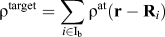 ${\rho ^{{\rm{target}}}} = \sum\limits_{i \in {{\rm{I}}_{\rm{b}}}} {{\rho ^{{\rm{at}}}}\left( {{\bf{r}} - {{\bf{R}}_i}} \right)}$, where the index i runs over all ions in region Ib, which represents the bulk-like electron density expected in region Ib. The QM charge density ρQM is then obtained as the outcome of a constrained DFT calculation in which the charge density ρQM is constrained to match the predetermined target charge density ρtarget within Ωc, i.e., the density constraint is ρQM(r) = ρtarget(r) in Ωc. Note that the constraint is not imposed on the entire region Ib because the electron density of region Ii extends into partial space of region Ib and should not be constrained. The constraint is imposed only in Ωc, which is computed self-consistently as the ionic positions are changed. Numerically, Ωc encompasses those points r satisfying min{ρtarget(r), ρMM(r)} > ρcf, where ρcf is a numerical cut–off parameter. We have shown that ρcf = 10−4 Å−3 is sufficient to yield the converged results for ρQM(r).Reference Zhang, Lu and Curtin22
Having specified the target charge density and the domain Ωc where the constraint is imposed, we now develop the associated constraint potential that is added as an “externally applied potential” to the KS Hamiltonian to drive the QM charge density toward the target charge density in Ωc. Following the method developed by Zhao et al.,Reference Zhao and Parr31,Reference Zhao, Morrison and Parr32 the constraint potential is given byReference Zhang, Lu and Curtin22
 $$\upsilon _{\rm{c}}^\lambda \left( {\bf{r}} \right) = \lambda \omega \left( {\bf{r}} \right)\int_{{\Omega _{\rm{c}}}} {{{{\rho ^{{\rm{QM}}}}\left( {\bf{r}} \right) - {\rho ^{{\rm{target}}}}\left( {{\bf{r'}}} \right)} \over {\left| {{\bf{r}} - {\bf{r'}}} \right|}}} {\rm{d}}{\bf{r'}}\quad ,$$
where λ is a penalty parameter. Since the constraint is only imposed in Ωc, the constraint potential should be localized to Ωc. We have introduced a cut off function ω(r) which is defined as
 $$\omega \left( {\bf{r}} \right) = \left\{ {\matrix{ 1 {{\rm{if}}} {\rho '\left( {\bf{r}} \right) > 2{\rho _{{\rm{cf}}}}} \cr {{{\rho '\left( {\bf{r}} \right)} \over {{\rho _{{\rm{cf}}}}}} - 1} {{\rm{if}}} {{\rho _{{\rm{cf}}}} \le \rho '\left( {\bf{r}} \right) \le 2{\rho _{{\rm{cf}}}}} \cr 0 {{\rm{if}}} {\rho '\left( {\bf{r}} \right) \lt {\rho _{{\rm{cf}}}}} \cr} \quad ,} \right.$$
where ρ′ = min{ρtarget(r), ρMM(r)}. The constraint potential  $\upsilon _{\rm{c}}^\lambda$ parameterized by λ is incorporated into the KS equation as an externally applied potential, so thatReference Zhang, Lu and Curtin22
 $$\left( { - {1 \over 2}{\nabla ^2} + V_{{\rm{eff}}}^{{\rm{KS}}} + \upsilon _{\rm{c}}^\lambda } \right)\left| {\phi _n^\lambda } \right\rangle = \varepsilon _n^{\rm{\lambda }}{\bf{S}}\left| {\phi _n^\lambda } \right\rangle \quad ,$$
where  $V_{{\rm{eff}}}^{{\rm{KS}}}$ is the usual KS effective potential including electron–electron, electron–ion, and exchange–correlation potentials. For a given λ, ρQM,λ is self-consistently determined by solving the KS equation. The resulting eigenvalues
 $\varepsilon _n^\lambda$ and eigenfunctions
 $\phi _n^\lambda$ with
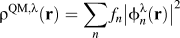 ${\rho ^{{\rm{QM}},\lambda }}\left( {\bf{r}} \right) = \sum\limits_n {{f_n}{{\left| {\phi _n^\lambda \left( {\bf{r}} \right)} \right|}^2}}$ (f n is the occupation number) are then obtained. The energy of the QM region E DFT[Ii + Ib] is thus calculated asReference Zhang, Lu and Curtin22
 $${E_{{\rm{DFT}}}}\left[ {{\rho ^{{\rm{QM}},\lambda }};{{\bf{R}}^{{\rm{QM}}}}} \right] = \sum\limits_n {{f_n}\varepsilon _n^\lambda } + {E_{{\rm{d}}{\rm{.c}}{\rm{.}}}}\left[ {{\rho ^{{\rm{QM}},\lambda }}} \right] + {\gamma _{{\rm{Ewald}}}}\left[ {{{\bf{R}}^{{\rm{QM}}}}} \right] - \int_{{\Omega _{\rm{c}}}} {{\rho ^{{\rm{QM}},\lambda }}\left( {\bf{r}} \right)\upsilon _{\rm{c}}^\lambda \left( {\bf{r}} \right){\rm{d}}{\bf{r}}\quad ,}$$
where E d.c. is the usual double-counting energy term and γEwald is the Madelung energy. The energy contribution of the constraint potential (as an external potential) is subtracted from the constrained DFT energy because E DFT[ρQM,λ; RQM] represents the energy of the QM region by itself.
There are two issues in the constrained DFT method: (i) determination of a sufficiently accurate target charge density ρtarget to represent the bulk-like charge density and (ii) implementation of the constraint potential in Eq. (18) that enforces the self-consistently determined ρQM,λ(r) to match ρtarget in Ωc. For issue (i), we use Eqs. (11) and (12) to generate the atomic charge densities ρat(r − Ri). Then the target charge density ρtarget is exact, within fitting errors by solving Eq. (11), for the perfect crystal. For the deformed crystal, the ion positions change but the electron densities attached to each ion do not change. However, properties of the approximate material that uses the electron density specified by ρtarget(r) in a non-self-consistent Kohn–Sham analysis yield a very accurate lattice constant, cohesive energy, and also bulk modulus (associated with deformation) as compared to the full self-consistent KS result.Reference Zhang, Lu and Curtin22 Thus, the target charge density gives a good representation of the true charge density and linear elastic material properties. For issue (ii), a constrained DFT calculation is converged if the resultant charge density is identical to the target charge density. In principle, Eq. (20) should be solved in the limit λ → ∞, but in practice, as λ increases, the ability to enforce the constraint is swamped by other numerical factors so that convergence cannot be obtained.Reference Zhao, Morrison and Parr32 To circumvent this problem, one could solve Eq. (20) self-consistently with a series of larger and larger λ values and then extrapolate the results to λ = ∞.Reference Zhao and Parr31 However, when a QM region contains hundreds of atoms, this method becomes impractical. In addition, we find that the self-consistent loops become increasingly difficult to converge with larger λ values. Our aim is to perform single self-consistent KS calculations with a sufficiently large value of λ that balances computational accuracy and efficiency. Under this consideration, we introduce the λ-dependent quantity,Reference Zhang, Lu and Curtin22
 $$C\left( \lambda \right) = {1 \over {2\lambda }}\int_{{\Omega _{\rm{c}}}} {\left[ {{\rho ^{{\rm{QM}},\lambda }}\left( {\bf{r}} \right) - {\rho ^{{\rm{target}}}}\left( {\bf{r}} \right)} \right]\upsilon _{\rm{c}}^\lambda \left( {\bf{r}} \right){\rm{d}}{\bf{r}}\quad ,}$$
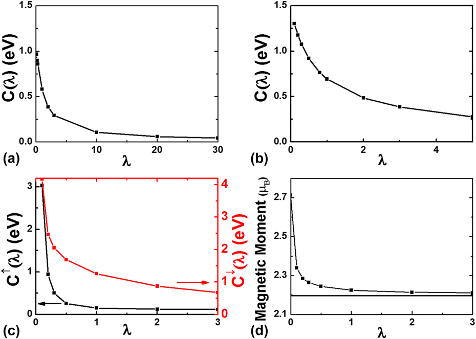
to quantify the difference between the resultant and target charge densities, weighted by the constraint potential over the constrained domain. C(λ) decreases with increasing λ and vanishes when λ = ∞. As shown in Fig. 3, we have determined that values of λ = 20, 5, and 2 are suitable for Al, Pd, and Fe, respectively. For magnetic materials such as Fe, a constraint is developed for each of the two independent spin densities.
C(λ) versus λ for three ideal systems (a) Al, (b) Pd, and (c) Fe. In (c), the black (red) curve represents the spin-up (spin-down) electrons. (d) The variation of the magnetic moment per atom as a function of λ for Fe. The horizontal line indicates the magnetic moment of a perfect lattice determined from the periodic DFT calculation. From Zhang et al.Reference Zhang, Lu and Curtin22

Finally, we consider the ionic force Fi = −∂E tot[Ii + Ib + II]/∂Ri on any ion i that emerges from the total energy formulation, Eq. (17). Forces on ions in region Ii only arise from the first term, E DFT[Ii + Ib] and thus are fully quantum mechanical in origin. Forces on ions in region II arise only from the second term, E MM[Ib + II] and thus are fully atomistic in origin. However, forces on ions in region Ib arise from a combination of DFT and MM energies. The disparity in DFT and MM energy functionals gives rise to coupling errors on force. As shown in Sec. II.A.2, the force errors are avoided by using a single method throughout the entire domain to compute the force in region Ib. Here, MM is used to calculate the forces on region Ib ions by −∂E MM[Ii + Ib + II]/∂R. Given these forces, the system is driven to a stable equilibrium structure by minimizing the ionic forces on all ions in the system. And a correction energy is then added into the total energy following Eq. (15).
C. Quasicontinuum DFT
1. Basic idea
In this section, we extend the QM/MM coupling to a multiscale QC approach. The goal is to combine the coarse-graining scheme of QCReference Tadmor, Ortiz and Phillips43,Reference Shenoy, Miller, Tadmor, Rodney, Phillips and Ortiz44 and the QM/MM coupling, leading to a multiscale QCDFT methodReference Peng, Zhang, Huang, Carter and Lu23,Reference Peng, Zhang, Huang, Carter and Lu45 that can simulate multimillion atoms effectively with KS-DFT or OFDFT as its sole energetics formulation. Here, we focus on the extension of the first QM/MM method to QCReference Peng, Zhang, Huang, Carter and Lu23; the second QM/MM method can be extended to the QC framework in the same manner and will not be duplicated here. The original QC method combines atomistic models with continuum theories and offers an advantage over conventional atomistic simulations in terms of computational efficiency.Reference Tadmor, Ortiz and Phillips43,Reference Shenoy, Miller, Tadmor, Rodney, Phillips and Ortiz44 The basic idea of the QC method is that atomistic processes of interest often take place in very small spatial domains, while the vast majority of atoms in the material can be described by well-established continuum theories. To exploit this fact, the QC method retains atomic resolution only where necessary and coarsens to a continuum description elsewhere. This is achieved in QC by replacing the full set of N atoms with a small subset of N r representative atoms or repatoms (N r ≪ N) that approximate the total energy through appropriate weighting.Reference Tadmor, Ortiz and Phillips43,Reference Shenoy, Miller, Tadmor, Rodney, Phillips and Ortiz44 The energies of individual repatoms can be computed in two different ways depending on their local deformation. Atoms experiencing large deformation gradients on an atomic scale are computed via a standard fully atomistic method. In QC, these atoms are called nonlocal atoms.Reference Tadmor, Ortiz and Phillips43,Reference Shenoy, Miller, Tadmor, Rodney, Phillips and Ortiz44 On the other hand, the energies of atoms experiencing a smooth deformation field are computed based on the deformation gradient G in their vicinity as befitting a continuum model. These atoms are called local atoms. The total energy of the system thus consists of two contributions,Reference Peng, Zhang, Huang, Carter and Lu23
 $$E_{{\rm{tot}}}^{{\rm{QCDFT}}} = {E^{{\rm{nl}}}}\left[ {{\rho ^{{\rm{tot}}}}} \right] + \sum\limits_{j = 1}^{{N^{{\rm{loc}}}}} {{n_j}E_j^{{\rm{loc}}}\left( {\left\{ {\bf{G}} \right\}} \right)\quad .}$$
Here, ρtot is the total electron density of the system; n j is the number of atoms that are represented by the jth repatom and  $E_j^{{\rm{loc}}}$ is the energy density associated with the jth repatom. There are N loc such local repatoms.
2. Implementation
To compute the energy and force in the local QC region, a finite element mesh is generated with each repatom on the vertices of the finite elements.Reference Tadmor, Ortiz and Phillips43,Reference Shenoy, Miller, Tadmor, Rodney, Phillips and Ortiz44 The energy and force of each local repatom are computed based on the strain energy density and the stress tensor of the finite elements which share the same repatom. According to the Cauchy–Born rule, the deformation gradient G is the same everywhere in a given finite element; thus the local energy density and the stress tensor for each finite element can be computed on a perfect crystal undergoing a uniform deformation defined by the deformation gradient G.
For the deformation gradient Gk associated with the kth element, a periodic OFDFT or KSDFT calculation can be performed to determine the strain energy density per unit cell E OF(Gk). The energy of the jth local repatom is thus a weighted sum of the strain energy E OF(Gk) of the surrounding finite elements,Reference Peng, Zhang, Huang, Carter and Lu23
 $$E_j^{{\rm{loc}}}\left( {\left\{ {\bf{G}} \right\}} \right) = \sum\limits_{k = 1}^{{M_j}} {{\omega _{jk}}{E_{{\rm{OF}}}}\left( {{{\bf{G}}_k}} \right)} \quad ,$$
where M j is the total number of finite elements shared by the jth repatom and ωjk is the weight associated with the kth finite element for the jth local repatom. The stress tensor of the kth element can be computed as followsReference Peng, Zhang, Huang, Carter and Lu23:
 $${\sigma _{{\rm{ab}}}} = {1 \over \Omega }\sum\limits_\nu {{{\partial {E_{{\rm{OF}}}}\left( {{{\bf{G}}_k}} \right)} \over {\partial {h_{{\rm{a}}\nu }}}}{h_{{\rm{b}}\nu }}\quad ,}$$
with Ω being the volume of the deformed unit cell and h ij denoting the ith Cartesian component of the deformed lattice vector h j. The force on the jth local repatom is obtained from the stress tensor of surrounding finite elements.Reference E and Lu41
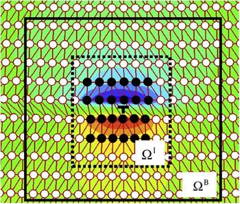
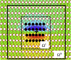
For the nonlocal QC calculations, the QM/MM approach is used. In QCDFT, region I consists of the nonlocal repatoms and region II includes the buffer atoms which are a combination of both “dummy” atoms and local repatoms in QC terminology, as shown in Fig. 4. The so-called “dummy” atoms, which are in the local region, are not independent degrees of freedom but rather slaves to the local repatoms. The position of a dummy atom is determined by the finite element interpolation from the nearby local repatom positions.Reference E and Lu41,Reference Liu, Lu, Chen and Kioussis42 The buffer ions and their charge densities provide the boundary conditions for the nonlocal calculation while the energy of the “dummy” atoms is still treated with the Cauchy–Born rule, consistent with their status. Hence, both the energy of the nonlocal atoms and the interaction energy between the nonlocal atoms and the surrounding buffer atoms are calculated by OFDFT. Typically, the buffer region consists of several atomic layers surrounding the nonlocal region. We associate each buffer ion in region II with a valence electron density (ρat) and a pseudopotential; both of them are constructed a priori and remain fixed. The nonlocal energy E nl as defined in Eq. (16) can be expressed asReference Peng, Zhang, Huang, Carter and Lu23
 $${E^{{\rm{nl}}}} = \mathop {\min }\limits_{{\rho ^{\rm{I}}}} \left\{ {{E_{{\rm{OF}}}}\left[ {{\rho ^{\rm{I}}};{{\bf{R}}^{\rm{I}}}} \right] + E_{{\rm{OF}}}^{{\mathop{\rm int}} }\left[ {{\rho ^{\rm{I}}},{\rho ^{{\rm{II}}}};{{\bf{R}}^{\rm{I}}},{{\bf{R}}^{{\rm{II}}}}} \right]} \right\}\quad .$$
Here, RI and RII denote atomic coordinates in regions I and II, respectively. The charge density of region I, ρI, is the degree of freedom and is determined self-consistently by minimizing the nonlocal energy functional. The charge density of region II, ρII, is defined as the superposition of atomic-centered charge densities ρat, which only changes upon the relaxation of region II ions.
The schematic diagram of domain partition in QCDFT with a dislocation as an example. The black and white spheres represent the nonlocal and buffer atoms, respectively. The dotted box represents ΩI and the solid box represents the periodic box ΩB. From Peng et al.Reference Peng, Zhang, Huang, Carter and Lu45

Although QCDFT utilizes the idea of QM/MM coupling, it does not involve any classical potentials (or force fields) in the formulation—the energy calculation of QCDFT is entirely based on OFDFT. This is an important feature and advantage of QCDFT, which represents a coarse-grained quantum simulation method.
III. APPLICATIONS TO METALLIC MATERIALS
In this section, we provide some examples where the QM/MM methods have been applied to understand fundamental physics in diverse material problems, including void formation, pipe diffusion along dislocation core, nanoindentation of thin films, hydrogen-assisted cracking, magnetism-induced plasticity, and stress controlled catalysis in metals. The QM/MM methods have proved particularly useful in mechanochemistry applications of metallic materials.
A. Void formation
Void formation due to irradiation, electromigration, or mechanical deformation in materials can significantly degrade their performance.Reference Hassan, Blanchard and Kulcinski46–Reference Seppala, Belak and Rudd48 Unfortunately, conventional computational approaches cannot provide accurate energetics for voids or vacancy clusters. On the one hand, first-principles calculations, although are rather accurate in terms of energetics, they are computationally too expensive to treat moderate or large vacancy clusters. Empirical atomistic simulations, on the other hand, are in general not accurate enough to compute the relevant energetics of the vacancy clusters. To overcome this challenge, we used the OFDFT-based QM/MM approach to compute the energetics of the vacancy clusters in Al and to correlate the tendency of void formation to the electron charge densities of the clusters.Reference Zhang and Lu49
According to the steady-state nucleation theory of voids,Reference Katz and Wiedersich50,Reference Clement and Woods51 the concentration of vacancy clusters with various sizes can be determined by their Gibbs free energies, consisting of formation enthalpy, formation entropy, and configurational entropy, under equilibrium between cluster sizes with the constraint of a constant supersaturation. At a constant pressure, the vacancy formation enthalpy can be approximated with the formation energy by using a large supercell in the energetic calculations. The formation energy of an n-vacancy cluster can be calculated as
 $$E_{n{\rm{v}}}^{\rm{F}} = E_{n{\rm{v}}}^{{\rm{tot}}}\left( {N - n} \right) - {{N - n} \over N}{E^{{\rm{tot}}}}\left( N \right)\quad ,$$
where  $E_{n{\rm{v}}}^{{\rm{tot}}}\left( {N - n} \right)$ is the total energy of the supercell containing N − n atoms with an n-vacancy cluster and E tot(N) is the total energy of the supercell containing N atoms in the perfect bulk configuration. The vacancy formation entropy
 $S_{n{\rm{v}}}^{\rm{F}}$ can be similarly defined. We can then determine the Gibbs binding free energy at temperature T as
 $$G_{n{\rm{v}}}^{\rm{B}} = \left( {nE_{{\rm{1v}}}^{\rm{F}} - E_{n{\rm{v}}}^{\rm{F}}} \right) - T\left( {nS_{{\rm{1v}}}^{\rm{F}} - S_{n{\rm{v}}}^{\rm{F}}} \right)\quad ,$$
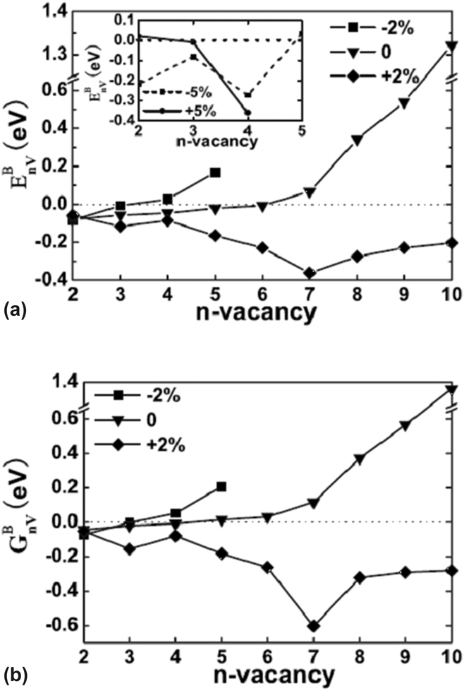
where the first term in parenthesis at the right-hand side is the binding energy of a n-vacancy cluster. The positive (negative) value of  $G_{n{\rm{v}}}^{\rm{B}}$ indicates that the n-vacancy cluster is thermodynamically stable (unstable) against a simultaneous dissociation into n monovacancies. We used the QM/MM approach to compute the binding energy and Gibbs binding free energy for n-vacancy clusters (n ranges from 2 to 10) as a function of hydrostatic pressures,Reference Zhang and Lu49 as shown in Fig. 5. We also revealed a correlation between the formation of vacancy-induced bonding cage and a negative and slowly increasing Gibbs free energy, which is responsible for void formation in fcc metals.
Binding energy (a) and Gibbs binding free energy at 300 K (b) of n-vacancy clusters in Al. 0, ±2%, and ±5% represent the percentage changes in lattice constant. From Zhang et al.Reference Zhang and Lu49

B. Pipe diffusion along dislocation core
Dislocation core can act as a fast path for diffusing atoms whose mobility can be orders of magnitude higher than in bulk diffusion and this phenomenon is referred as “pipe diffusion”. Pipe diffusion can affect many kinetic processes in materials, including creep,Reference Pandey, Mishra, Paradkar and Mahajan52 dynamic-strain aging,Reference Brechet and Estrin53 crystallization,Reference Luo, Shen and Wang54 and electromigration.Reference Baker, Joo, Knaub and Arzt55 Motivated by an experiment which has observed “giant diffusivity” of Si interstitial pipe diffusion in Al,Reference Legros, Dehm, Arzt and Balk56 we have carried out the OFDFT-based QM/MM simulations to examine the pipe diffusion of Si interstitials along an edge dislocation in Al.Reference Zhang and Lu57
We have applied the QM/MM approach to determine the core structure of the edge dislocation in pure Al, which provides hints on plausible locations of the interstitial Si atoms. Thanks to the planar structure of the dislocations, we can use the relative atomic displacements across the slip plane to represent the edge and screw components of the strain field, respectively. The derivative of the relative displacement with respect to the atomic positions gives rise to the corresponding dislocation density.Reference Lu, Kioussis, Bulatov and Kaxiras58 The double peak in the dislocation density plot suggests that the dislocation is dissociated into two Shockley partials whose position is represented by the peaks.Reference Zhang and Lu57
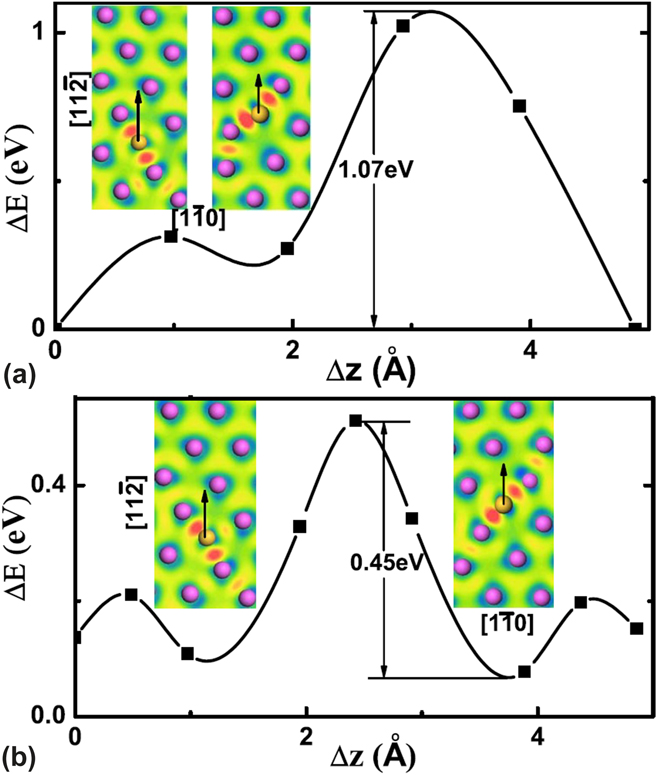
Next, we introduce an interstitial Si atom at the dislocation core. To simulate the pipe diffusion along the dislocation core, we need to determine the stable energetic positions for the interstitial Si atom. Here, we take the left partial (LP) as an example to study the pipe diffusion as the two partials are equivalent. We find that the interstitial Si atom prefers to stay at the same atomic layer of the neighboring Al atoms, owing to the chemical bonding between them, which dominates the effect of volume expansion.Reference Zhang and Lu57 The similar observation is also found in the stacking fault (SF) ribbon where the Si atom is located at the same layer of the Al atoms as shown in Fig. 6. Furthermore, between the stable positions at the LP and the SF, the Si atom is found to be energetically more stable in the LP with an energy difference of 0.08 eV.Reference Zhang and Lu57
The energy profile for the diffusion path along LP (a) and SF (b). The left (right) contour plots represent the bonding charge density around the Si atom for the initial state (saddle state), and the contour scale ranges from −0.07 Å−3 (blue) to 0.09 Å−3 (red). The arrow indicates the diffusion direction. The magenta and yellow spheres represent Al and Si atoms, respectively. From Zhang et al.Reference Zhang and Lu57

Figure 6 summarizes the diffusion paths and barriers of Si along both LP and SF. The diffusing Si atom follows approximately a sinusoidal trajectory that reflects the periodicity of the underlying lattice. For diffusion along the LP, the diffusion energy profile exhibits two peaks with an energy barrier of 1.07 eV.Reference Zhang and Lu57 The QM/MM energy barrier is in excellent agreement with the experimental value of 1.12 eV.Reference Legros, Dehm, Arzt and Balk56 The diffusion energy profile along the SF is symmetric with a much smaller energy barrier of 0.45 eV.Reference Zhang and Lu57 Therefore, the SF ribbon could provide a fast pathway for diffusion which increases the diffusivity by three orders of magnitude relative to the partial dislocation core at 700 K. In other words, we have predicted a “faster pipe diffusion” which occurs along the SF ribbon. The reason the faster pipe diffusion was not observed experimentally may be due to the fact that the SF configuration (with Si) has a slightly higher energy (0.08 eV) than the LP configuration (with Si). The higher energy could lead to a probability ratio of 1–4 for the Si atom ending up at SF versus LP at 700 K (at room temperature, the odds reduce to 1 to 25).
C. Nanoindentation of thin film
Nanoindentation is a powerful experimental probe which can evaluate the mechanical responses of small volumes of materials, such as thin films and can estimate the critical stress required to nucleate dislocations in an otherwise defect-free material.Reference Fischer-Cripps59 We have used the QCDFT method to study solid solution strengthening effect on dislocation nucleation in Al thin film in the presence of Mg impurities during nanoindentation.Reference Peng, Zhang, Huang, Carter and Lu45,Reference Peng, Zhang and Lu60
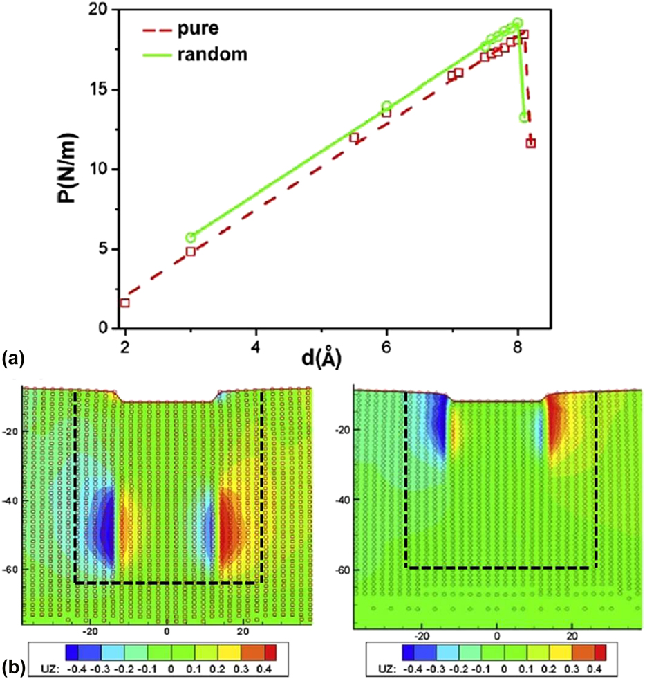
The load–displacement curve is typical observable for nanoindentation and is widely used in both experiment and theory. In particular, it is conventional to identify the onset of incipient plasticity with the first drop in the load–displacement curve during indentation. Here, the load is given in N/m, normalized by the length of the indenter in the out-of-plane direction. As detailed in Ref. Reference Peng, Zhang and Lu60, the load–displacement curve in pure Al shows a linear relation followed by a drop at d = 8.2 Å, indicated by the dashed line in Fig. 7. The drop indicates a homogeneous nucleation of dislocations beneath the indenter corresponding to the onset of plasticity. A pair of straight edge dislocations are nucleated at x = ±13 Å and y = −50 Å. In Fig. 7, we present the out-of-plane (or screw) displacement of the nonlocal repatoms. The nonzero screw displacement of the edge dislocations suggests that each dislocation is dissociated into two 1/6 〈112〉 Shockley partials bound by an SF with a width of about 19 Å.Reference Peng, Zhang and Lu60 The activated slip planes are {111} planes, which are adjacent to the edges of the indenter. The slope for the linear part of the curve is 27.1 GPa and the critical load for the homogeneous dislocation nucleation is 18.4 N/m, corresponding to a hardness of 7.3 GPa.Reference Peng, Zhang and Lu60
(a) Load–displacement plot for the nanoindentation of the Al thin film with a rigid rectangular indenter: pure Al (red squares) and randomly distributed Mg impurity system (green circles). (b) The out-of-plane displacement obtained from the pure (left) and with Mg impurities (right) QCDFT calculations. The QM region is outlined by dashed lines. The circles represent the repatoms and the displacement ranges from −0.4 (blue) to 0.4 (red) Å. From Peng et al.Reference Peng, Zhang and Lu60

For a random distribution of Mg impurities in the Al thin film, the load–displacement curve exhibits a linear relation up to a depth of 8.0 Å, followed by a drop at d = 8.1 Å, as shown by the solid line in Fig. 7. The slope of the initial linear part of the load–displacement curve is 26.7 GPa, very close to the corresponding pure Al value.Reference Peng, Zhang and Lu60 The maximum load in the linear region is 19.2 N/m, corresponding to a hardness of 7.6 GPa, which is 0.3 GPa greater than the pure Al system. A pair of Shockley partial dislocations is nucleated at x = −13 Å, y = −25 Å and x = 13 Å, y = −22 Å, respectively, as shown in Fig. 7. The drop in the applied load owing to the incipient plasticity is 5.9 N/m. The fact that the critical load and the hardness of the Al–Mg alloy are greater than those of the pure Al demonstrates that the Mg impurities are responsible for the solid solution strengthening of the Al thin film.Reference Peng, Zhang and Lu60 The presence of Mg impurities also hinders the formation of full edge dislocations and as a result, only partial dislocations are nucleated and they are pinned near the surface as shown in Fig. 7.
D. Hydrogen-assisted cracking
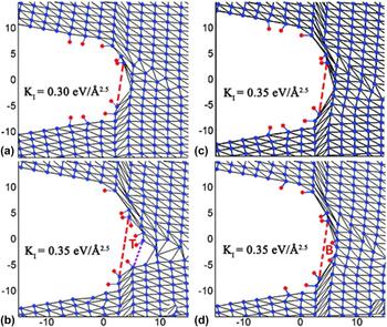
The presence of H is known to promote crack growth in a variety of technologically important materials.Reference Lynch, Gangloff and Somerday61 To shed light on the atomistic mechanisms underlying H embrittlement of metals, we have used QCDFT to examine the H-assisted cracking in Al.Reference Sun, Peng and Lu62 Previous calculations have showed that the Al–Al bonds can be attacked by H with a significant charge transfer from Al to H.Reference Lu, Zhang, Kioussis and Kaxiras63–Reference Apostol and Mishin65 Hence, we consider two H adsorption sites at the crack tip in the QCDFT simulations: B site on the bridge center of an Al–Al bond and T site right on top of an Al atom, as shown in Fig. 8. The H atom at the B site forms an Al–H–Al bond, whereas the H atom at the T site forms an Al–H bond. At the crack tip, H atoms can be adsorbed on the up-surface (U), down-surface (D), and front-surface (F). To examine all these possibilities, we have studied eight different cases in Ref. Reference Sun, Peng and Lu62, labeled from (A) to (H) as in Table I. The primary quantities of interest here are the critical stress intensity for dislocation emission, K IC, and the crack opening at the stress intensity of 0.3 eV/Å2.5, Δ. As shown in Table I, we find that H-assist cracking occurs only when H atoms are adsorbed at the T site of the crack front-surface; H concentration at ∼0.2 ML is sufficient to lead to crack growth as shown in case D.Reference Sun, Peng and Lu62 In contrast, H atoms adsorbed on the side surfaces (both up- and down-surfaces) cannot yield crack growth. Furthermore, H atoms at the T site and B site on the crack front-surface are found to modify the behavior of dislocation nucleation at the crack tip.Reference Sun, Peng and Lu62
(a) Cleavage of the first atomic layer at the crack tip; the second atomic layer becomes the new front-surface subsequently. (b) Cleavage of the second atomic layer when H atoms are adsorbed on the T sites of the fresh front surface. No cleavage of the second atomic layer for (c) without H atoms on the fresh front-surface and (d) H atoms adsorbed on the B sites of the fresh front surface. The red and purple dotted lines represent the first and second atomic layers, respectively. From Sun et al.Reference Sun, Peng and Lu62

Summary of K IC and Δ for eight crack configurations. Symbols in the configuration reflect the adsorbed H positions, e.g.,  ${\rm{F}}_6^{\rm{B}}$ means that there are six H atoms adsorbed on the bridge or B site at the crack front-surface. N H is the total number of adsorbed H atoms at the crack tip. From Sun et al.Reference Sun, Peng and Lu62

The QCDFT calculations provide the following picture for H-assisted cracking in metals: (i) At the crack front-surface, H adsorbed on the T sites could attack Al–Al bonds which results in the fracture in the first atomic layer as shown in Fig. 8; the second atomic layer then emerges as the new front-surface. (ii) The H atoms at the original front-surface and/or the side surfaces can diffuse to the fresh front-surface. (iii) With increasing loading, H on the T sites of the fresh front-surface continues attacking the Al–Al bonds at the second atomic layer as shown in Fig. 8. Steps (ii) and (iii) repeat for a continuous crack growth. To confirm the key assumption that only the H atoms on the T sites can contribute to step (iii), we examine two contrasting cases with and without H atoms at the B sites of the fresh front-surface.Reference Sun, Peng and Lu62 At the stress intensity of 0.35 eV/Å2.5, the fracture of the second atomic layer occurs only when H atoms are adsorbed on the T sites as shown in Fig. 8 with a significant opening of Δ = 3.9 Å. On the other hand, in the two contrasting cases, the crack does not grow as indicated in Fig. 8.
The simulations explain why a sufficiently high H concentration at the crack tip, which is difficult to realize in Al under normal conditions, is in fact unnecessary for H embrittlement, resolving a long-standing puzzle in H embrittlement of Al. The presence of H at the active sites is found to be more important than the average concentration of H for embrittlement of Al. Therefore, H embrittlement could be mitigated if the T sites are blocked or made less stable by alloying, heat treatment, or other means. The understanding and control of crack tip chemistry holds the key to rational design of embrittlement-resistant materials for which multiscale quantum mechanical modeling could be an invaluable tool.
E. Magnetic impurities on dislocation core structure in Fe
Ferritic steels are prime candidates for structural components of fusion reactors, in which Cr is a critical alloying element contributing to improving the materials’ resistance to corrosion, irradiation, and swelling.Reference van der Schaaf, Gelles, Jitsukawa, Kimura, Klueh, Mosloang and Odette66,Reference Malerba, Caro and Wallenius67 Hence, a fundamental understanding of how Cr changes the dislocation core properties of α-Fe would have important scientific and technological relevance. To this end, we have used the second QM/MM approach to examine the effect of Cr impurity on the core structure of an edge dislocation in α-Fe.Reference Zhang and Lu68
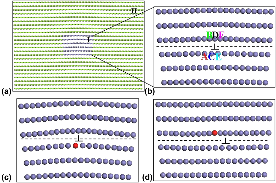
As shown in Fig. 9, the QM/MM simulation of the edge dislocation consists of two regions: the QM region (region I) containing the dislocation core with/without a Cr impurity and the MM region (region II) consisted of the rest of the system. The edge dislocation has a Burgers vector of b = 1/2 〈111〉 on the {110} slip plane. The dislocation core is initially placed at the center of the region I as shown in Fig. 9. We have considered two substitutional sites for the Cr impurity at the dislocation core: one is at the tension site below the slip plane and the other is at the compression site above the slip plane, as depicted in Fig. 9.
(a) Partition of the entire system into region I (blue spheres) and region II (green spheres, partially shown). (b) Atomic structure of region I for the edge dislocation in α-Fe. Dislocation structure with a Cr impurity occupying at (c) the tension site and (d) the compression site. The red spheres represent the Cr atom and the inverted ‘T’ symbol denotes the center of the dislocation. The dashed line indicates the slip plane. From Zhang et al.Reference Zhang and Lu68

We find that the Cr impurity can significantly modify the dislocation core structure of α-Fe.Reference Zhang and Lu68 When Cr takes the C site at the tension side, the dislocation core bends upward and the Cr repels the neighboring Fe atoms as shown in Fig. 9. The total energy difference between Cr at the C site and the A site is 0.1 eV, indicating an energy barrier of 0.1 eV for the dislocation to be depinned from Cr at the C site. When Cr occupies the D site at the compression side, a spontaneous dislocation glide takes place and the dislocation core translates about 2/3b away from Cr as illustrated in Fig. 9. It is further revealed that the strain-dependent magnetic interaction is responsible for the changes in the dislocation core structure.Reference Zhang and Lu68 When Cr takes the tension side of the slip plane, the Cr–Fe magnetic interaction is repulsive, which lowers the dislocation energy and pins the dislocation. When Cr is at the compression side of the slip plane, the magnetic Cr–Fe interaction is attractive, which increases the dislocation energy and promotes the dislocation to break away from Cr.
F. Stress-controlled catalysis
Controlling nanoparticle (NP) surface strain, i.e., compression (or stretch) of surface atoms, is an important approach to tune its surface chemistry and to optimize its catalytic activities. For example, Pt-based core/shell NPs have been shown to exhibit outstanding catalytic activities in the oxygen reduction reaction (ORR), an important cathodic reaction in low-temperature polymer electrolyte membrane fuel cells and metal–air batteries.Reference Gasteiger and Markovic69,Reference Debe70 The lattice mismatch between the core material and Pt shell could induce strain on the shell, and a judicious selection of the core materials offers an attractive means to tune the ORR activity and selectivity on the core/shell NPs.Reference Wang, Inada, Wu, Zhu, Choi, Liu, Zhou and Adzic71–Reference Stamenkovic, Fowler, Mun, Wang, Ross, Lucas and Markovic75 Therefore, computational screening and search for an optimal combination of core/shell materials with superior ORR activities is highly desirable.
The multiscale QM/MM is well-poised to model catalysis on the core/shell NPs in which QM is applied to the reactive region while the long-range strain field of the NPs is captured by MM. We have used the second QM/MM approach to study ORR on the Pt–Cu core/shell NPs.Reference Zhang and Lu76 The Pt–Cu core/shell NPs consist of Pt shell and Cu core, modeled by icosahedrons with twenty (111) facets, as shown in Fig. 10. We have considered four NPs with d = 3.2, 4.8, 6.4, and 8.0 nm, corresponding to 923, 2869, 6525, and 12,431 atoms, respectively.Reference Zhang and Lu76 For each NP, three Pt shell thicknesses (t = 0.6, 0.8, and 1.0 nm) are examined, corresponding to three, four, and five Pt atomic layers, respectively. It has been well-established that the oxygen surface adsorption energy E O is a good descriptor of ORR activity in both pure metals and alloys.Reference Stamenkovic, Mun, Mayrhofer, Ross, Markovic, Rossmeisl, Greeley and Norskov77,Reference Norskov, Rossmeisl, Logadottir, Lindqvist, Kitchin, Bligaard and Jonsson78 We find that the optimal or target value of E O should be 0.2 eV higher than that on the flat Pt(111) surface. The goal of the study is to design core/shell particles so that E O approaches as closely as possible to the target value. The E O values as a function of d and t for both core/shell and pure Pt NPs are shown in Fig. 10. It is found that the pure Pt NPs cannot reach the target value of E O for the reasonable particle sizes.Reference Zhang and Lu76 On the other hand, the Pt–Cu core/shell NPs could offer higher ORR activities as both the black and red curves intersect the target line in Fig. 10. All these results are consistent with the corresponding experimental findings.Reference Wang, Inada, Wu, Zhu, Choi, Liu, Zhou and Adzic71
(a) Partition of the entire system into the interior QM region Ii (red and pink spheres), the boundary QM region Ib (green spheres), and the MM region II (blue spheres). d is the NP diameter. (b) The atomic structure of the Pt–Cu core/shell NP. Brown and blue spheres represent Cu and Pt atoms, respectively. t is the thickness of the Pt shell. (c) E O on the Pt–Cu core/shell and pure Pt NPs. (d) Correlation between E O and the surface strain for the NPs and the Pt flat surface. There exists a universal linear relation between E O and the strain. From Zhang et al.Reference Zhang and Lu76

Most importantly, we found a universal linear relation between E O and surface strain for all materials studied here including core–shell particle, pure particles, and flat surface, as shown in Fig. 10. This universal relation could be used to screen core/shell NPs for ORR based on the following strategy.Reference Zhang and Lu76 First, we would determine the distribution of surface strain on the core/shell NPs by using inexpensive MM simulations; QM simulations are not necessary here. Next, we can estimate E O from the strain values according to the universal linear relation. Finally, we can assess ORR activity based on the E O values. Using this strategy, we predict that Fe, Co, Ni, and Cu can be used as core materials to improve the ORR activity, whereas Ag and Au are not good for the Pt-based core/shell NPs. Our predictions have been confirmed by experiments.Reference Zhang, Zhang, Jiang, Zhu, Guo, Su, Lu and Sun79 The QM/MM method has also been used to study ORR on Pd based core/shell NPs.Reference Chen, Zhang and Lu80
IV. SUMMARY AND OUTLOOK
The challenge in simulations of materials science and engineering is that real materials usually exhibit phenomena on one scale that require a very accurate and computationally expensive description, and phenomena on another scale for which a coarser description is satisfactory and, in fact, necessary to avoid prohibitively large computations. QM/MM represent a multiscale modeling strategy that combines the strengths of QM and MM modeling and strives to achieve a balance among accuracy, efficiency, and realistic description. The presence of delocalized electronic states in metallic materials invalidates the popular coupling schemes across the interface and renders QM/MM modeling of metals particularly challenging. In this paper, we reviewed recent advances in QM/MM modeling of metallic materials and how these QM/MM methods can be used to address a wide range of problems, ranging from void formation, pipe diffusion along dislocation core, nanoindentation of thin films, hydrogen-assisted cracking, magnetism-induced plasticity to stress-controlled catalysis in metals.
In terms of future development of QM/MM modeling for metallic materials, we can envision three directions. First, there is significant progress in the development of more accurate interatomic potentials based on machine learning representations of DFT potential energy surfaces.Reference Bartok, Payne, Kondor and Csanyi81–Reference Li, Kermode and De Vita85 Interatomic potentials thus developed can yield accurate energetic and structural properties in MM calculations. As a result, the mismatch between the QM and MM determined energy and force is much smaller and so are the coupling errors. These interatomic potentials could drastically improve the fidelity and the robustness of QM/MM modeling. Second, we envision more accurate and efficient schemes for the construction of electron charge densities in MM region. Progress could be made in improving the basis functions to expand the charge density and/or better numerical procedures to minimize the objective functions. Ideas to speed up the convergence of constrained DFT calculations are of crucial importance in the second QM/MM method. Going beyond the approximation that the MM charge density depends only on the ionic positions in the MM region could enable the QM/MM methods to capture charge transfer across the QM/MM interface. And this development is expected to improve the accuracy of QM/MM methods, particularly in metals where long-range charge redistributions may take place. Recently, a QM/MM method that allows the exchange of electron densities across the QM/MM interface has been developed for organic molecular systemsReference Zhang and Lin86–Reference Pezeshki and Lin88; the generalization of such method to metals is particularly interesting. Third, the present QM/MM methods have been confined in static relaxations. No molecular dynamic simulations have been attempted so far with the QM/MM methods for two reasons: (i) ab initio MD for metallic systems is computationally expensive; (ii) there is a lack of general coupling schemes which ensure energy and momentum conservation in MD simulations. Effort to remedy this problem has been discussed in an excellent review on this subject.Reference Bernstein, Kermode and Csanyi3 Essential to the problem is the inconsistence between the total energy and the atomic forces in the QM/MM formulations. There are two ways of formulating the total energy and forces in a QM/MM method. One can define the total energy of a QM/MM system to consist of separate contributions from the QM and MM regions, in addition to the interaction between the two regions, as in this paper. However, the atomic forces thus calculated would inevitably contain coupling errors (or “mismatch”) across the QM/MM boundary, owing to the intrinsic incompatibility between the QM and MM forces. Such force errors are sometime called “ghost forces”, originally discussed in the context of the QC method.Reference Shenoy, Miller, Tadmor, Rodney, Phillips and Ortiz44 To mitigate the problem, one can introduce a correction energy contribution to the total energy, and its derivative (i.e., correction force) can partially offset the “ghost forces”.Reference Bernstein, Kermode and Csanyi3,Reference E, Lu and Yang40–Reference Liu, Lu, Chen and Kioussis42,Reference Shenoy, Miller, Tadmor, Rodney, Phillips and Ortiz44 Conversely, one can define the atomic forces of a QM/MM system and as a result, the “ghost forces” do not arise. However, doing so would lead to an ill-defined total energy and in practice, one has to forgo the total energy in the QM/MM simulations. In QM/MM MD simulations, the presence of the “ghost forces” and/or the lack of a well-defined total energy would result in problems such as continuously increased temperature in MD. Future development in this directionReference Bernstein, Kermode and Csanyi3,Reference Duster, Wang, Garza, Miller and Lin89 could prove extremely valuable not only to QM/MM modeling but also to multiscale modeling in general.
ACKNOWLEDGMENT
We acknowledge the support of Office of Naval Research (N00014-15-1-2092).